Sequential Monte Carlo Methods for High-Dimensional Inverse Problems: A case study for the Navier-Stokes equations
Abstract
We consider the inverse problem of estimating the initial condition
of a partial differential equation, which is only observed through
noisy measurements at discrete time intervals. In particular, we focus
on the case where Eulerian measurements are obtained from the time
and space evolving vector field, whose evolution obeys the two-dimensional
Navier-Stokes equations defined on a torus. This context is particularly
relevant to the area of numerical weather forecasting and data assimilation.
We will adopt a Bayesian formulation resulting from a particular regularization
that ensures the problem is well posed. In the context of Monte Carlo
based inference, it is a challenging task to obtain samples from the
resulting high dimensional posterior on the initial condition. In
real data assimilation applications it is common for computational
methods to invoke the use of heuristics and Gaussian approximations.
As a result, the resulting inferences are biased and not well-justified
in the presence of non-linear dynamics and observations. On the other
hand, Monte Carlo methods can be used to assimilate data in a principled
manner, but are often perceived as inefficient in this context due
to the high-dimensionality of the problem. In this work we will propose
a generic Sequential Monte Carlo (SMC) sampling approach for high
dimensional inverse problems that overcomes these difficulties. The
method builds upon “state of the art” Markov chain Monte Carlo
(MCMC) techniques, which are currently considered as benchmarks for
evaluating data assimilation algorithms used in practice. SMC samplers
can improve in terms of efficiency as they possess greater flexibility
and one can include steps like sequential tempering, adaptation and
parallelization with relatively low amount of extra computations.
We will illustrate this using numerical examples, where our proposed
SMC approach can achieve the same accuracy as MCMC but in a much more
efficient manner.
Keywords: Bayesian inverse problems, Sequential Monte Carlo, data
assimilation, Navier-Stokes
1 Introduction
We consider the inverse problem of estimating the initial condition of a dynamical system described by a set of partial differential equations (PDEs) based on noisy observations of its evolution. Such problems are ubiquitous in many application areas, such as meteorology and atmospheric or oceanic sciences, petroleum engineering and imaging (see e.g. Bennett (2002); Evensen (2009); Talagrand and Courtier (1987); Stuart (2010); Cotter et al. (2013); Kaipio and Somersalo (2005)). In particular, we will look at applications mostly related to numerical weather forecasting and data assimilation, where one is interested in prediction of the velocity of wind or ocean currents. There, a physical model of the the velocity vector field is used together with observed data, in order to estimate its state at some point in the past. This estimated velocity field is then used as an initial condition within the PDE to generate forecasts. In this paper we focus on the case where the model of the evolution of the vector field corresponds to the two-dimensional (2D) Navier-Stokes equations and the data consists of Eulerian observations of the evolving velocity field originating from a regular grid of fixed positions. Although the inverse problem related to the Navier-Stokes dynamics may not be as difficult as some real applications, we believe it can still provide a challenging problem where the potential of our methods can be illustrated. Furthermore, the scope of our work extends beyond this particular model and the computational methods we will present are generic to inverse problems related with dynamical systems.
In a more formal set-up, let and be given normed vector spaces. A statistical inverse problem can be formulated as having to find an unknown quantity that generates data :
where is an observation operator and denotes a realization of the noise in the observation; see Kaipio and Somersalo (2005) for an overview. In a least squares formulation, one may add a Tikhonov-Phillips regularization term to ensure that the problem is well posed (see e.g. Cotter et al. (2013); Law and Stuart (2011); Stuart (2010)) in which case one seeks to find the minimizer:
where are trace class, positive, self-adjoint operators on respectively and . In addition, one may also be interested in quantifying the uncertainty related to the estimate . This motivates following a Bayesian inference perspective which is the one adopted in this work. Under appropriate conditions (to be specified later; Stuart (2010)) one can construct a posterior probability measure on such that Bayes rule holds:
where is the prior and is the likelihood. The prior is chosen to be a Gaussian probability measure (i.e. a normal distribution on with mean and covariance operator ) as implied by prior knowledge on the smoothness or regularization considerations. The likelihood, , is a density w.r.t some reference measure on and is obtained from the statistical model believed to generate the data. For example, one may use
if a Gaussian additive noise model is adopted.
In this paper we will consider to be the unknown initial condition of the PDE of interest. We will model the observations as a vector of real random variables, , and assume is an appropriate Hilbert space. Thus, the observation operator is closely related to the semigroup of solution operators of the PDE, , which maps a chosen initial condition to the present state at time . It is straightforward both to extend Bayesian methodology for these spaces (Stuart (2010)) and to also ensure that necessary differentiability and smoothness conditions are being enforced with regards to the evolution of the vector field via the appropriate choice of the prior measure. We will also work with periodic boundary domains, which is a convenient choice that allows solving PDEs numerically using a spectral Galerkin method with Fast Fourier Transforms (FFTs). Notice that here we are confronted with an infinite-dimensional problem as is a function space, but in practice a high-dimensional discretization (or mesh) is used. Still it remains as an important requirement that any computational method should be able to cope with an arbitrary fine discretization, i.e. that it is robust to mesh refinement.
A plethora of methods have appeared in the literature to tackle such inverse problems. Usually these adopt various heuristic approximations when new data points are assimilated. The first successful attempt in this direction of algorithms was based on optimization and variational principles (Le Dimet and Talagrand (1986); Sasaki (1958)). Later, these ideas were combined with Gaussian approximations, linearizations and Kalman-type computations in Talagrand and Courtier (1987) leading to the popular 3DVAR and 4DVAR. Another popular method is the ensemble Kalman filter (enKF), which is nowadays employed by an increasing number of weather forecasting centers; see Evensen (2009) for an overview. Although these methods have been used widely in practice, an important weakness is that their use is not well justified for non-linear problems and it is hard to quantify under which conditions they are accurate (with the exception of linear Gaussian models; Le Gland et al. (2011)). A different direction that overcomes this weakness is to use Monte Carlo computations that make full use of Bayes rule to assimilate data in a principled manner. In this paper we will refer to these methods as ‘exact’ given the resulting estimation error will diminish by using more Monte Carlo samples and also in order to distinguish with the above methods that use heuristic approximations. Recently, exact Markov chain Monte Carlo (MCMC) methods suitable for high dimensional inverse problems have been proposed in the literature (Beskos et al. (2008); Cotter et al. (2013); Law (2012)). This class of MCMC algorithms can be shown to be much more accurate than the popular data assimilation algorithms mentioned earlier (see Law and Stuart (2011) for a thorough comparison). However, the improvement in performance comes at a much greater computational cost, limiting the effect of the method to providing benchmarks for evaluating data assimilation algorithms used in practice.
In this paper, we aim to improve in terms of the efficiency of obtaining Monte Carlo samples for Bayesian inference. We will use these accurate MCMC methods as building blocks within Sequential Monte Carlo (SMC) samplers (Chopin (2002); Del Moral et al. (2006)). Our work builds upon recent advances in MCMC/SMC methodology and we will propose a SMC sampler suitable for high-dimensional inverse problems. SMC methods have been very successful in a wide range of relatively low-dimensional applications (Doucet et al. (2001)) and their validity has been demonstrated by many theoretical results (see Del Moral (2004) for an exhaustive review). However, they are widely considered to be impractical for high-dimensional data assimilation applications. We believe that this is true only when they are implemented naively or in an inappropriate context, e.g. using for inverse problems standard particle filtering algorithms intended for stochastic dynamics. Evidence for this claim can be provided by recent success of SMC in high-dimensional applications (Jasra et al. (2011); Schäfer and Chopin (2013)) as well as recent theoretical results with emphasis on high dimensional problems (Beskos et al. (2013a, b); Schweizer (2012)).
We will propose an efficient algorithm based on the algorithm in Chopin (2002). We will generate weighted samples (called particles) from a sequence of target probability measures, , that starts from the prior, , and terminates at the posterior of interest (i.e. ). This is achieved by a combination of importance sampling, resampling and MCMC mutation steps. Several important challenges arise when trying to use this approach for the high-dimensional problems of interest in this paper:
- Overcoming
-
weight degeneracy: when the amount of information in an assimilated data-point is overwhelming then the importance weights will exhibit a very high variance. For instance at the -th step of the algorithm (when targeting ) the observations of the velocity field about to be assimilated might exhibit a highly peaked likelihood function relative to the previous target (and current proposal), .
- Constructing
-
effective MCMC mutation kernels: the availability of MCMC kernels with sufficiently mixing properties is well-known to be critical for algorithmic efficiency of SMC (Del Moral (2004)). This is extremely challenging in high dimensions since the target distributions are typically comprised of components with widely varying scales and complex correlation structures.
- Effective
-
design and monitoring of algorithmic performance: insufficient number of particles and MCMC mutation steps or inefficient MCMC kernels might lead to a population of particles without the required diversity to provide good estimates. Even in such an undesirable situation standard performance indicators such as the Effective Sample Size (ESS) can give satisfactory values and a false sense of security (this has been noted in Chopin (2002)). Hence the development and use of reliable criteria to monitor performance is required and these should be easy to compute using the particles.
In contrast to standard MCMC procedures, SMC samplers possess a great amount of flexibility with design elements that can be modified according to the particular problem at hand. Understanding some of the statistical properties of the posterior of interest can be used to design an appropriate (and possibly artificial) target sequence as well as constructing MCMC mutation steps with adequate mixing. To overcome the difficulties mentioned above we will propose to:
-
•
employ sequential and adaptive tempering to smooth peaked likelihoods by inserting an intermediate target sequence between and . At each step of the algorithm, the next temperature will be chosen automatically based on information from the particles as proposed in Jasra et al. (2011). In particular for our problem, adaptive tempering will not increase the total computational cost too much, when more amount of tempering is performed at earlier stages of the algorithm, which require shorter runs of the expensive numerical solutions of the PDE.
-
•
use the particles at each stage of the algorithm and adapt the MCMC steps to the structure of the target. Regarding this point it will be crucial to understand how to construct MCMC kernels robust to high dimensions (as in Cotter et al. (2013)).
-
•
use a statistic to measure the amount of diversity (jitter) of the particles during the MCMC mutation. We will use a particular standardized square distance travelled by the particles during the mutation, which to the best of our knowledge has not been used before. Good values for this criterion might be chosen by requiring a minimum amount of de-correlation.
- •
Indeed, our contribution will be to combine the above points to design a generic and efficient SMC algorithm that can be used for a variety of inverse problems of interest to the data assimilation community. We will demonstrate the performance of the proposed scheme numerically on the inverse problem related to the Navier-Stokes equations, but we expect similar performance in other problems such as the ones described in Cotter et al. (2013).
The organization of the paper is as follows. In Section 2 we formulate the inverse problem related to the Navier-Stokes equations that will be used in this paper. In Section 3 we present the MCMC sampling procedure of Beskos et al. (2008); Cotter et al. (2013) and a basic SMC sampling method. In Section 4 we will extend the SMC methodology for high dimensional inverse problems. In Section 5 we present two numerical examples with the inverse problem for the Navier-Stokes equations: in the first one SMC appears to achieve the same accuracy as MCMC at a fraction of the computational cost; in the second one it is unrealistic to use MCMC from a computational perspective, but SMC can provide satisfactory numerical solutions at a reasonable computational cost. Finally, in Section 6 we present a discussion with some possible extensions and some concluding remarks.
2 Problem formulation
In this section we will give a brief description of the Navier-Stokes equations defined on a torus, specify the observation mechanism and present the posterior distribution of interest for the initial condition. We will later use the problem formulated in this section as a case study for the proposed SMC algorithm for inverse problems.
2.1 Navier-Stokes Equations on a Torus
We will first set up the appropriate state space and then present the dynamics.
2.1.1 Preliminaries
Consider the state (or phase) space being the 2D-torus, , with being a point on the space. The initial condition of interest is a 2D vector field . We set , where and denotes vector/matrix transpose. We will define the vorticity as:
with the (slightly unusual) convention that clock-wise rotation leads to positive vorticity. Let denote the magnitude of a vector or complex variate. For a scalar field we will write . We will also consider the vector Laplacian operator:
and, for functions , the operator:
Define the Hilbert space:
and let be the closure of with respect to the norm in . Let also denote the Leray-Helmholtz orthogonal projector. An appropriate orthonormal basis for is comprised of the functions:
where and . So corresponds to a (bivariate) frequency and the Fourier series decomposition of an element is written as:
for the Fourier coefficients , with denoting complex conjugate. Notice that since is real-valued we will have .
Also we define to be the Stokes operator; note that is diagonalized in in the basis with eigenvalues where . Fractional powers of the Stokes operator can then be defined by the diagonalization. For any , we define as the operator with eigenvalues and eigenfunctions and the Hilbert spaces as the domain of , that is the set of such that .
2.1.2 The Navier Stokes equations
The Navier-Stokes equations describe Newton’s laws of motion for an incompressible flow of fluid defined on . Let the flow be initialized with and consider the case where the mean flow is zero. We will denote the time and space varying velocity field as , and this is given as follows:
where is the viscosity parameter, is the pressure function, an exogenous time-homogeneous forcing. We assume periodic boundary conditions:
Applying the projection to , we may write the equations in the form of an ordinary differential equation (ODE) in :
| (1) |
where the symmetric bi-linear form is defined as:
Intuitively, projects an arbitrary forcing into the space of incompressible functions . See Robinson (2001); Foias et al. (2001) for more details. Let denote the semigroup of solution operators for the equation (1) through time units. We also define the following discrete-time semigroup, corresponding to time instances , of lag and :
with the conventions , and .
2.2 A Bayesian Framework for the Initial Condition
We will model the data as noisy measurements of the evolving velocity field on a fixed grid of points, , for . These are obtained at regular time intervals that are time units apart. So the observations will be as follows:
where is constant and is initialized by the unknown ‘true’ initial vector field, . To simplify the expressions, we set:
Performing inference with this type of data is referred to as Eulerian data assimilation. The likelihood of the data, conditionally on the unknown initial condition , can be written as:
| (2) |
where a normalizing constant that does not depend on .
We will also consider the following family of priors:
| (3) |
with hyper-parameters affecting the roughness and magnitude of the initial vector field. This is a convenient but still flexible enough choice of a prior; see Da Prato and Zabczyk (2008, Sections 2.3 and 4.1) for an introduction to Gaussian distributions on Hilbert spaces. Indeed, when considering the Fourier domain, we have the real function constraint for the complex conjugate coefficients (), so we split the domain by defining:
We will impose that for . Since the covariance operator is determined via the Stokes operator , we have the following equivalence when sampling from the prior:
That is, admits the the following Karhunen-Loève expansion:
| (4) | |||
| (5) |
Thus a-priori, the Fourier coefficients with are assumed independent normally distributed, with a particular rate of decay for their variances as increases.
Adopting a Bayesian inference perspective, we need to construct a posterior probability measure on :
| (6) |
where is the normalization constant. Due to the generality of the state space, some care is needed here to make sure that under the chosen prior, the mappings possess enough regularity (i.e. they are -measurable) and hence the change of measure is well defined. For this reason we present below a proposition from Cotter et al. (2009) for this Eulerian data assimilation problem:
Proposition 1.
Assume that . Consider the Gaussian measure on with , . Then the probability measure is absolutely continuous with respect to with Radon–Nikodym derivative written in (2). In addition, a Maximum-a-Posteriori (MAP) estimate of the initial condition exists in the sense that attains an infimum in .
Proof.
The first part is Theorem 3.4 of Cotter et al. (2009). The second statement follows from the same paper by verifying Theorem 2.7 with Lemmata 3.1-3.2 and noting that is the Cameron-Martin space of by Lemma 4.3; for more details see the discussion after Theorem 3.4. ∎
Notice that condition is necessary and sufficient for to be a trace-class operator, thus also for the infinite-dimensional Gaussian measure to be well-defined; see e.g. Da Prato and Zabczyk (2008, Proposition 2.18). In this paper we will use a zero mean function for the prior, but this is done purely for the sake of simplicity. In fact, Proposition 1 is proven in Cotter et al. (2009) for with the mean functions . In addition, we note that even though in (2) will be obtained numerically in practice on a finite dimensional mesh, Proposition 1 can be extended to the posterior defined on the corresponding finite dimensional approximation for ; we refer the interested reader to Theorems 2.4 and 4.3 in Cotter et al. (2010).
3 Monte Carlo Methods for the Inverse Problem
In this section we present some Monte Carlo algorithms that can be used for inverse problems such as the one involving the Navier-Stokes dynamics formulated in Section 2. We will present first a well-established MCMC method applied in this context and then outline a basic general-purpose SMC sampling algorithm. We postpone the presentation of our proposed method for the next Section. There we will combine strengths from both the algorithms in this section to address the complex structure of the high-dimensional posteriors of interest in this paper.
Remark 1.
We emphasize again that the algorithms presented in both this and the next section are ‘exact’ (as also mentioned in the Introduction). By ‘exact’ we mean that the estimation errors are purely due to the finite number of Monte Carlo samples and can be made arbitrarily small. The methods are based on solid theoretical principles and can loosely speaking make full use of Bayes rule to assimilate the observations. This is in contrast to heuristic methods that invoke Gaussian approximations and Kalman type computations. Although these are commonly used in practice for high dimensional applications, they are not theoretically justified for non-linear dynamics (Le Gland et al. (2011)).
3.1 A MCMC Method on the Hilbert Space
MCMC is an iterative procedure for sampling from , where one simulates a long run of an ergodic time-homogeneous Markov chain that is -invariant111We will use throughout the convention to denote the -th iteration of any MCMC transition kernel.. After a few iterations (burn-in) the samples of this chain can be treated as approximate samples from . There are many possible transition kernels for implementing MCMC chains, but we will only focus on some algorithms that have been carefully designed for the posteriors of interest in this paper and seem to be particularly appropriate for Hilbert-space-valued measures arising as change of measure from Gaussian laws. Other standard MCMC algorithms (e.g. Gibbs, Random-Walk Metropolis) have been successfully used in high-dimensional applications; see e.g. Gilks et al. (1996). Nevertheless, in our context the posteriors possess some particularly challenging characteristics for MCMC:
- i)
-
they lack a hierarchical modeling structure. When this is present, conditional independencies of the coefficients are often exploited using Gibbs-type samplers that attempt updates of a fraction (or block) of Fourier coefficients (conditional to the remaining ones) at each iteration. Here such a structure is not present and implementation of conditional updates would require calculations over all coefficients (or dimensions), making Gibbs-type schemes not useful in practice.
- ii)
-
they are targeting an infinite-dimensional state space (in theory). In practice a high dimensional approximation (mesh) will be used, but we still require from a method to be valid for an arbitrary mesh size and hence robust to mesh refinement. This is not the case for standard Random-Walk-type algorithms that typically deteriorate quickly with the mesh size; see Hairer et al. (2011) for more details.
- iii)
-
information in the observations is not spread uniformly over the Fourier coefficients. A-posteriori these can have very different scaling ranging from the very low frequencies (where the support of the posterior can change drastically from the prior) to the very high ones (where the support of the posterior may closely resemble the prior). All these different scales cannot be easily determined either analytically or approximately making it difficult for MCMC algorithms to adjust their proposal’s step-sizes in the many different directions of the state space.
-
•
Run a -invariant Markov chain as follows:
-
•
Initialize . For :
-
1.
Propose:
-
2.
Accept with probability:
(7) otherwise .
-
1.
Considerations i) and ii) have prompted the development of a family of global-update MCMC algorithms, which are well-defined on the Hilbert space (and thus robust upon mesh-refinement). In Algorithm 1 we present such an algorithm222The notation is being used within the algorithm. corresponding to a Metropolis accept-reject scheme that has appeared earlier in Neal (1999) as a regression tool for Gaussian processes and in Beskos et al. (2008); Cotter et al. (2013); Stuart (2010) in the context of high-dimensional inference. In direct relevance to the purposes of this paper, Algorithm 1 has been applied in the context of data assimilation and is often used as the ‘gold standard’ benchmark to compare various data assimilation algorithms as done in Law and Stuart (2011). One interpretation why the method works in infinite dimensions is that Step 1 of Algorithm 1 provides a proposal transition kernel that preserves the Gaussian prior , while the posterior itself will be preserved using the accept/reject rule in Step 2. In contrast, standard Random-Walk Metropolis proposals (of the type ) would provide proposals of a distribution which is singular with respect to the target , and will thus be assigned zero acceptance probability. In practice, when a finite-dimensional approximation of is used, both the standard MCMC methods and Algorithm 1 will have non-zero acceptance probability, but in the limit only Algorithm 1 is valid. The mixing properties of the standard MCMC transition kernels will also diminish quickly to zero upon mesh-refinement (in addition to the acceptance probability), whereas this is not true for Algorithm 1 (Hairer et al. (2011)).
As a limitation, it has been noted often in practice that a value of very close to is needed (e.g. will be used later on) to achieve a reasonable average acceptance probability (say ). This is due to the fact that the algorithm is optimally tuned to the prior Gaussian measure , whereas the posterior resembles closely only at the Fourier coefficients of very high frequencies. This leads to small exploration steps in the proposal and relatively slow mixing of the MCMC chain, which means that one needs to run the chain for an excessive number of iterations (of the order ) to get a set of samples with reasonable quality. In addition, each iteration requires running a PDE solver until time to compute in Step 2, so the approach is very computationally expensive. To sum up, although Algorithm 1 has provided satisfying results in many applications (Cotter et al. (2013)), there is still a great need for further algorithmic development towards improving the efficiency of Monte Carlo sampling.
Remark 2.
More elaborate MCMC proposals have appeared in Law (2012) that can achieve better performance regarding consideration iii) above. There the proposals are based on some approximations of the posterior, , following the ideas in Martin et al. (2012). The method in Law (2012) has appeared in parallel to the work presented here and contains interesting ideas that are definitely relevant to the material in this paper. Nevertheless, as it is currently under closer investigation it will not be considered here or later on in our comparisons in Section 5.
3.2 A generic SMC Approach
We proceed by a short presentation of SMC and refer the reader to Chopin (2002); Del Moral et al. (2006) for a more thorough treatment. Instead of a single posterior over all observations, consider now a sequence of probability measures defined on such that and is a prior as in (3). For example, one may consider the natural ordering of the observation times to construct such a sequence. Indeed, consider the likelihood of the block of observations at the -th epoch:
Note that as increases so does the computational effort required to compute due to using a numerical PDE solution to evaluate . Given that the observation noise is independent between different epochs, we define a sequence of posteriors as follows:
| (8) |
This forms a bridging sequence of distributions between the prior and the posterior, which also admits a Karhunen-Loève expansion:
| (9) |
where compared to (4)-(5), are now correlated random variables from some unknown distribution. Note the particular choice of in (8) is a natural choice for this problem. In fact, there are other alternatives involving artificial sequences and introduction of auxiliary variables (and the extension in the next section are an example for this; see Del Moral et al. (2006) for some more examples). The SMC algorithm will target sequentially each intermediate , which will be approximated by a weighted swarm of particles (or samples). This is achieved by a sequence of selection and mutation steps (see Del Moral (2004, Chapter 5)):
- Selection
-
step: At the -th iteration say we have available equally weighted samples of , denoted . These will be used as importance proposals for and are assigned the incremental (normalized) weights:
The weighting step is succeeded by a resampling step so as to discard samples with low weights. The particles are resampled probabilistically with replacement according to their weights .
- Mutation
-
step: Carrying out only selection steps will eventually lead to degeneracy in the diversity of the particle population. During each successive resampling step, only few parent particles will survive and copy themselves. Thus, some ‘jittering’ of the population is essential to improve the diversity. These jittering steps should maintain the statistical properties of and are hence chosen to be a small number of -invariant MCMC iterations. For example, one could consider using a few times Steps 1-2 of Algorithm 1 but with the complete likelihood replaced with (although we will discuss later why this is not recommended).
In Algorithm 2 we present the general purpose SMC algorithm that that has appeared in Chopin (2002). For the resampling step, we have used to denote the distribution of the indices of the parent particles. For instance, one may copy offsprings according to successful counts based on the multinomial distribution of the normalized weights (this is the approach we follow in this paper). Recall also that denotes the -th particle approximating and in this paper this will be thought as a concatenated vector of the real and imaginary parts of the Fourier coefficients in (or its finite truncation). Upon completion of Step 2 one obtains particle approximations for :
where denotes the Dirac point measure at . The convergence and accuracy of these Monte-Carlo approximations have been established under relatively weak assumptions and in various contexts; see Del Moral (2004) for several convergence results. Note that most steps in the algorithm allow for a trivial parallel implementation and hence very fast execution times; see Lee et al. (2010); Murray et al. (2013) for more details. In addition, the resampling step is typically only performed when an appropriate statistic (commonly the effective sample size (ESS)) will indicate its necessity; e.g. when ESS will drops below a prescribed threshold:
When not resampling, particles keep their different weights (and are not all set to ), which are then multiplied with the next incremental weights. In Chopin (2002) the author uses the particle population to design (that) either as a standard random walk or as an independent Metropolis-Hastings sampler based on particle approximation .
-
•
At , for sample .
-
•
Repeat for :
-
1.
Selection:
-
(a)
Importance Sampling: weight particles , .
-
(b)
Resample (if required):
-
i.
Sample offsprings .
-
ii.
Set and , .
-
i.
-
(a)
-
2.
-invariant mutation: update , , where .
-
1.
As Algorithm 2 is based on sequential importance sampling its success relies on:
-
•
resembling closely in order to avoid the weights degenerating.
-
•
providing sufficient jitter to the particles in order to counter the lost diversity due to resampling. For instance, the number of MCMC iterations used needs to be enough for particles to spread around the support of .
These issues become much more pronounced in high dimensions. We will extend the SMC methodology to deal with these issues in the following section.
4 Extending SMC for High Dimensional Inverse Problems
One advantage of SMC is its inherent flexibility due to all different design elements such as the sequence or the kernels . In high dimensional applications such as data assimilation a user needs to design these carefully to obtain good performance. In addition, monitoring the performance also includes some challenges itself. We will deal with these issues in this section.
Firstly, recall the equivalence between representing the initial vector field by its Fourier coefficients and vice versa:
In this section will be treated again as the concatenated vector of the real and imaginary part of its Fourier coefficients. In theory, this vector is infinite-dimensional, but in practice it will be finite (but high) dimensional due to the truncation in the Fourier space used in the numerical PDE solver. We will sometimes refer to the size of the implied mesh, , informally as the dimensionality of .
SMC as in Algorithm 2 will need to satisfy some requirements to be effective. As already mentioned at the end of Section 3, broadly speaking these are:
-
•
each selection step should not deplete the particle population by excessively favoring one or relatively few particles. This deficiency can arise in the context of importance sampling when likelihood densities are overly peaked, so that only a few particles give non-trivial likelihood values to the corresponding observation.
-
•
each mutation step should sufficiently jitter the particles, so that the population will span most of the support of the target measure. Ideally, the mixing properties of the MCMC kernels assigned to do this should not degrade with increasing .
We will address the first point by altering the sequence of SMC targets and the second point by proposing improved MCMC kernels compared to simple modifications of Algorithm 1.
First we need to ensure that the importance sampling weights (in Step 1 of Algorithm 2) are ‘stable’ in the sense that they exhibit low variance. For high dimensional inverse problems it is expected that this is not the case when the sequence is defined as in (8). We will modify the sequence of target distributions so that it evolves from the prior to the posterior more smoothly or in a more ‘stable’ manner. One way to achieve this is by bridging the two successive targets and via intermediate tempering steps as in Neal (2001). So one can introduce a (possibly random) number, say , of artificial intermediate targets between and :
| (10) |
where
| (11) |
are a sequence of user-specified temperatures. The accuracy of SMC when using such tempering schemes have been the topic of study in Beskos et al. (2013b, a); Giraud and Del Moral (2012); Schweizer (2012); Whiteley (2012). From these works the most relevant to the present high-dimensional setup are Beskos et al. (2013a, b). There in a slightly simpler setup the authors demonstrated that it is possible to achieve the required weight stability with a reasonable computational cost, when the sequence of targets varies slowly and the MCMC mutation steps mix well for every target in the bridging sequence.
For the SMC sequence implied jointly by (8) and (10), in Section 4.1 we will present an adaptive implementation for choosing the next temperature on-the-fly (Jasra et al. (2011)) and in Section 4.2 propose improved MCMC mutation kernels that use particle approximations for each .
4.1 Stabilizing the Weights with Adaptive Tempering
A particularly useful feature of using tempering within SMC is that one does not need to choose for every bridging sequence and before running the algorithm. In fact these can be decided on-the-fly using the particle population as it was originally proposed in Jasra et al. (2011). Suppose at the moment the SMC algorithm is about to proceed to iteration (the -th tempering step between and ). The MCMC mutation step for temperature has just completed and let be equally weighted particles333Here denotes the concatenated real vector of real and imaginary Fourier coefficients in for the -th particle targeting . Often in the discussion we interpret as a probability measure on a similar real vector . approximating as defined in (10). The next step is to use as importance proposals for . The incremental weights are equal to , so if has been specified, they can be also written as:
| (12) |
Now from the expression in (12) it follows that one can choice of by imposing a minimum quality for the particle population after the weighting, e.g. a minimum value for the ESS. Therefore we can use the particles to specify as the solution of the equation:
| (13) |
If one should set and proceed to the next tempering sequence leading to . Solving the above equation for can be easily implemented using an iterative bisection on for the scalar function . There is now only one user-specified parameter to be tuned, namely . This adaptive tempering approach of Jasra et al. (2011) has been also used successfully in Schäfer and Chopin (2013); Zhou et al. (2013). In Zhou et al. (2013) one may also find an alternative choice for the quality criterion instead of the ESS. Finally, assuming sufficient mixing for the MCMC mutation steps, the accuracy of adaptive tempering has been studied in Giraud and Del Moral (2012).
Remark 3.
The exposition uses intermediate tempering between the natural target sequence defined in (8). If one is not interested in the intermediate posterior using part of the data then it is possible to attempt tempering directly on . Similarly, if each is a high dimensional vector, then one could define intermediate targets between each or some elements in and temper between these targets. In the latter case caution must be taken to avoid unnecessary intermediate tempering steps due to outliers in the observations. In any of these cases we remark the presented methodology still applies.
4.2 Improving the Mixing of MCMC Steps with Adaptive Scaling
We proceed by considering the design of the MCMC mutation steps to be used between tempering steps. We will design a random-walk-type method, tuned to the structure of the target distributions, by combining two ingredients:
- (a)
-
we will use current information from the particles to adapt the proposal on-the-fly to the target distribution.
- (b)
-
we will distinguish between high and low frequencies for the MCMC formulation. This is a consideration specific to inverse problems related to dissipative PDEs, where the data often contains more information about the lower frequencies.
We will look for a moment at the MCMC mutation kernel of Algorithm 2. Recall the correspondence between an element in and its Fourier coefficients. To remove the effect of different scaling for each Fourier coefficient (due to the different variances in prior) we will consider the bijection
as implied by (4)-(5) for or (9) for . As a result a-priori, , for all are i.i.d. samples from . The proposal in Step 1 of Algorithm 1 written in terms of is:
| (14) |
This would be an excellent proposal when the target is the prior (or close to it). When such a proposal is used within MCMC transition kernels for Step 2 of Algorithm 2, then the mixing of the resulting mutation kernels will rapidly deteriorate as we move along the sequence of bridging distributions between and . The assimilated information from the observations will change the posterior densities for each relative to the prior. In particular, often the data will contain a lot of information for the Fourier coefficients located at low frequencies, thereby shrinking their posterior variance. Thus, at these low frequencies the update in (14) will require a choice of very close to 1 for the proposal to have a non-negligible chance to remain within the domain of the posterior and hence deliver non-vanishing acceptance probabilities. At the same time such small steps will penalize the mixing of the rest of the Fourier coefficients with relatively large posterior variances. This is a well known issue often seen in practice (Law (2012)) and somehow the scaling of the random walk exploration for each frequency needs to be adjusted to the shape of the posterior it is targeting.
We will adapt the proposal to the different posterior scalings in the coefficients using the particles. Assume that the algorithm is currently at iteration , where the importance sampling step with proposals from in (10) has been completed and we have the weighted particle set approximating . We will construct the MCMC mutation kernel (so that ) as follows. With a slight abuse of notation, we denote by the bivariate real vector comprised of the real and imaginary part of the -th Fourier coefficient of , where and . We estimate the marginal mean and covariance of the th Fourier coefficient under the current target in the sequence as follows:
| (15) |
The estimated moments , (and the corresponding Gaussian approximation of the posterior) will be used to provide the scaling of the step size of the random walk for each . Let be the collection of particles obtained after resampling with replacement according to the weights . In the MCMC mutation step we can use the following proposal instead of (14):
| (16) |
Notice that in (16) we propose to move the real and imaginary parts of the Fourier coefficients separately for each frequency . This requires computing only the mean and covariances of the -th marginal of . Other options are available, involving jointly estimating higher-dimensional covariance matrices (for the joint vector involving every ). However, caution is needed because of the Monte Carlo variance in estimating high dimensional covariances, when the number of particles is moderate (as it will be the case for the computationally expensive numerical examples in this paper). A pragmatic option in this case is to use only the diagonal elements of the joint covariance estimator or possibly include some off-diagonal terms where (partial) correlations are high.
Chopin (2002) has applied such adaptive ideas advocating both the use of an independence sampler as well as a standard random walk (e.g. ). There more emphasis is placed towards the independence sampler, as it was possible to use asymptotic statistical theory to suggest that the posterior converges with to a multivariate normal. Thus, accurate estimation of the covariance matrix would eventually result to high acceptance probabilities. This approach is better suited for low dimensions (and a high number of particles), but in high dimensions it makes sense to opt for a local-move proposal like (16). In high dimensions it is extremely hard to capture very accurately the structure of the target as in Chopin (2002) simply by using estimates of very high-dimensional mean vectors and covariance matrices based on moderate number of Monte Carlo samples. This intuition was confirmed also in Schäfer and Chopin (2013), where a different local-move approach was proposed for high dimensional binary spaces using random walks from appropriate parametric families of distributions.
The second ingredient of the proposed MCMC mutation kernel involves distinguishing between low and high frequencies. In particular, we will use the proposal of (16) for a window of the Fourier coefficients with relatively low frequencies and the standard proposal of (14) that uses the prior for the higher frequencies. We have found empirically that this thrifty hybrid approach gives a better balance between adaptation and variability caused by Monte Carlo error in estimating empirical covariances. We will use the proposal of (16) for coefficients with frequencies in the rectangular window defined as:
| (17) |
where . It would certainly be possible to use an alternative definition for . For instance, we could include all frequencies such that , but this is not expected to make a considerable difference in terms of computational efficiency. The idea here is that for high enough frequencies the marginal posterior of the Fourier coefficients should be very similar to the prior, i.e. the observations are not very informative for these frequencies. Hence, in high frequencies one might as well use the standard proposal of (14) and still attain good enough mixing.
-
1.
Initialize (when in Step of Algorithm 4 set ). Let , be known approximations for all . Choose .
-
2.
For :
-
(a)
For , propose the update:
for propose the update:
-
(b)
Compute forward dynamics and likelihood functions .
-
(c)
With probability:
(18) accept the proposal and set ; otherwise set . We use:
(19) (20) (21) -
(a)
-
3.
Output as a sample from .
The proposed MCMC kernel is presented in Algorithm 3. For simplicity, in the notation we omit subscripts when writing for . We also use subscripts , to refer to collection of concatenated vectors of real/imaginary parts of Fourier coefficients in and respectively and is a unit matrix. Notice, that even with adaptation, a few MCMC iterations (denoted by ) might be required to generate enough jittering for the populations of particles (e.g. ). Another interesting feature is the different choice of step sizes and used inside and outside the window respectively. These step sizes might be still close to when the target posteriors admit a very complex correlation structure. Nonetheless, in Section 5 we will present numerical examples where substantially lower values can be used to produce reasonable acceptance ratios () than when only proposals from the prior are used for all the frequencies . The increased exploration steps will contribute significantly towards more efficiency in the Monte Carlo sampling procedure.
Remark 4.
In the Navier-Stokes dynamics (1), for appropriate choice of the spectrum of the time evolving vector field tends to concentrate at low frequencies. This is common for many dissipative PDEs. Loosely speaking, the dissipation will transfer energy from high to low frequencies until enters the attractor of the PDE. In cases where the likelihood is formed by noisy observations of , the resulting posteriors will tend to be more informative at lower frequencies. Finally, a good initial choice of could be implied by the spacing of the observation grid, but this is a heuristic specific to Eulerian data assimilation.
Remark 5.
The acceptance probability in (18) follows from the usual Metropolis-Hastings accept-reject principle. Compared with the acceptance probability in (7) the terms involving arise to account for the different proposal at the low frequencies. If we used the proposal in (16) for all , it would be necessary to ensure somehow that the acceptance ratio is well defined and non-zero. In this case, one should make sure that the corresponding infinite sums in (20)-(21) are finite. A related practical issue is that any mismatch of the proposed samples with due to Monte Carlo error can result to many rejected samples. Using a finite deals with these issues and one might also need to use higher values of when increases.
We note here that we could opt to use a ‘smooth’ window for instead of a window with a sharp edge like (17). A possible implementation could be to modify the proposal to:
where
with being user-specified sequences converging to as . The impact of different choices of the rate of decay of these sequences is yet to be investigated, but this is beyond the scope of this paper.
4.3 The Complete Algorithm
-
•
At , for sample .
-
•
For
-
1.
For compute forward dynamics and .
-
2.
Set and .
-
3.
While
-
(a)
Increase by .
-
(b)
(Compute temperature)
IF , set
ELSE compute such thatusing a bisection on .
-
(c)
(Compute weight) for :
-
(d)
(Compute moment estimates and ) for :
-
(e)
(Resample) let . For set and .
-
(f)
(-invariant mutation) for , sample (see Algorithm 3).
-
(a)
-
4.
Set .
-
1.
The complete SMC algorithm is presented in Algorithm 4. The proposed algorithm computes the temperatures and the scaling of the MCMC steps on-the-fly using the evolving particle populations. To improve the mixing of the mutation steps, we use the new adaptive MCMC kernel in Algorithm 3 and distinguish between high and low frequencies. After the completion of Step 4 of Algorithm 4, the particles can be used to approximate the intermediate posteriors ; this is emphasized in Step 4 by denoting when . In addition, when the resampling steps can be omitted whenever , as mentioned in Section 3.2. Although this is not taken into account in Algorithm 4, this extension involves storing (when ) each individual weight from Step 3(c) as , so that at the subsequent weighting step (only) they can get multiplied to the un-normalized weight: (similarly to Step 1(a) of Algorithm 2).
Although standard SMC methods have a well-developed theoretical framework for their justification, this literature is much less developed in the presence of the critical adaptive steps considered in Algorithm 4. When both adaptive scaling of MCMC steps and adaptive tempering are considered together, we refer the reader to Beskos et al. (2013c) for asymptotic convergence results (in ).
As regards the computational cost, for each MCMC mutation at iteration , we need to run the PDE numerical solver times from up to the current time . Therefore, the total computational cost is proportional to , where depends on the random number of tempering steps. In fact, this cost is significantly reduced when more tempering steps are required for small values of . Finally, the memory requirements are as there is no need to store past particles at each step of the algorithm.
4.4 Monitoring the performance: towards an automatic design
Although SMC is a generic approach suitable for a wide class of problems, this flexibility also means that the user has to select many design elements. Firstly, one must decide the target sequence , which often is imposed by the problem at hand as in (8). If such a natural sequence is not available, adaptive tempering can be used directly on as explained in Remark 3. The remaining design choices here are and . The choice of can be determined based on the available computational power and memory. Assuming the user can afford repeated algorithmic runs, then a useful rule of thumb is to avoid increasing after the resulting estimates do not change much. We proceed by outlining different measures of performance for each of the remaining tuning parameters:
-
1.
For , we recommend that they should be tuned so that at time the acceptance ratio in (18) averaged over the particles has a reasonable value, e.g. . Having said that, the average value of the acceptance ratio should be recorded and monitored for the complete run of the SMC. The same applies for the ESS, which will also reveal how much tempering is used during the SMC run.
-
2.
It is critical to choose so as to provide sufficient diversity in the particle population. A question often raised when using SMC samplers is whether a given value of (or a particular MCMC mutation more generally) is adequate. We propose the following measure for monitoring the jitter in the population for each frequency and each intermediate step of the algorithm :
(22) We remark that the statistic has not been used before for SMC to the best of our knowledge. Of course, monitoring every value of is not necessary, and one could in practice choose a small number of representative frequencies from their complete set. In addition, as increases, will converge to . Hence, statistical intuition can explain what requirements we should pose for , e.g. that it should be at least above . In our context the MCMC mutation steps are applied to jitter the population at each of the many steps of the SMC sampler. The role of the MCMC steps here is very different than in a full MCMC sampler, where the number of MCMC steps have to be large enough for ergodic theory to apply.
-
3.
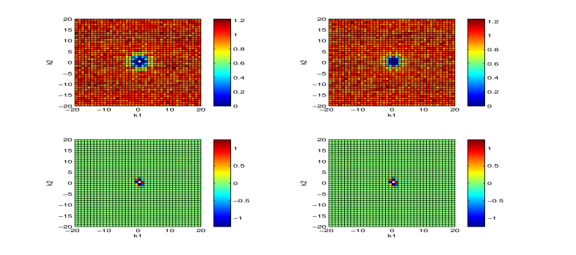
It is also possible to empirically validate whether the chosen value for , the half-width of , was appropriate. A revealing plot here is the two-dimensional heat map of the ratio of the variance of the posterior to the variance of the prior against . should include as much as possible the region where this ratio is significantly less than , e.g. say less than .
All the above criteria can be used to empirically evaluate algorithmic performance during or after a SMC run with a particular set of tuning parameters. Fortunately, SMC does not require complicated convergence diagnostics similar to MCMC.
A particularly interesting point is that summaries like the average acceptance ratio, the statistic , or the ratio of the posterior to prior variance can be also be potentially used within decision rules to determine , and adaptively on-the-fly. This can be implemented similarly to how the ESS is used for adaptively choosing the tempering temperatures. To choose for instance one may keep using MCMC iterations until the median of over a number of representative frequencies reaches a pre-specified value. For an option can be to increase/decrease them by a given fraction according to the values of the empirical average acceptance ratio over the particle population as done in Jasra et al. (2011). Similarly, can vary according to the ratio of the estimated posterior variances to the prior ones on the boundary of . These aforementioned guidelines or other similar ideas can lead towards a more automatic implementation of the proposed SMC algorithm. Although we believe investing effort towards this direction is definitely important, this lies beyond the scope of this paper. So, in the numerical examples to follow the performance measures mentioned here are used as monitoring tools but not as means to adapt more tuning parameters.
Remark 6.
We should clarify that adaptation in this paper is of a very different nature than what is commonly referred to as adaptive MCMC in the literature, e.g. Andrieu and Thoms (2008). There, the MCMC tuning parameters such as in Algorithm 1 vary according to the history of the sample path of the MCMC trajectory. This method is intended for long MCMC runs and care needs to be taken to ensure that appropriate diminishing adaptation conditions are satisfied. Here the interest is only to jitter the population. The MCMC mutations have different invariant measures at each and are based on very few standard MCMC iterations, which conditional on the whole particle population are independent for each particle.
5 Numerical Examples
We will use numerical solutions for the Navier-Stokes PDE in (1) given an initial condition. We employ a method based on a spectral Galerkin approximation of the velocity field in a divergence-free Fourier basis (Hesthaven et al. (2007)). The convolutions arising from products in the nonlinear term are computed via FFTs on a grid with additional anti-aliasing using double-sized zero padding (Uecker (2009)). In addition, exponential time differencing is used as in Cox and Matthews (2002), whereby an analytical integration is used for the linear part of the PDE, , together with an explicit numerical Euler integration scheme for the non-linear part, .
In this section we will present two numerical examples using two different synthetic data-sets obtained from some corresponding true initial vector fields, . The first example will use Data-set A consisting of few blocks of observations obtained at close time intervals (small ), but each block is obtained from a dense observation grid (high ). For this example we will compare the performance of our method with benchmark results from the MCMC approach described in Algorithm 1. For the second example we will use Data-set B, a longer data-set with blocks of observations spaced apart by longer time periods , each originating from a sparser observation grid (low ). In both cases the total number of observations of the vector field will be the same and . We summarize these details in Table 1.
| Data-set A | , , | |
|---|---|---|
| Data-set B | , , |
The two data-sets are synthesized using the numerical PDE solver described above. In both cases we have set:
where we remind the reader that is the viscosity, the external forcing, and the observation noise variance. Adjoint PDE solvers will be used in the sense that the same numerical solver is used for synthesizing the data and in the Monte Carlo inference algorithms.
| Algorithmic | number of calls of PDE solver | execution time | |
|---|---|---|---|
| Parameters | with time length (divided by ) | ||
| MCMC Dataset A | 9 days | ||
| SMC Dataset A | 3 days | ||
| no parallelization | |||
| SMC Dataset A | 7.4 hours | ||
| with parallelization | |||
| SMC Dataset B | 3.5 days | ||
| with parallelization |
In Table 2 we summarize the computational cost of the algorithms used in our experiments. The table presents the number of times a PDE solution is required and the total execution time. We do not provide an MCMC benchmark for Data-set B as the more expensive PDE solver needed in this case would result in an enormous execution time for Algorithm 1. For SMC, we will present results from an implementation of Algorithm 4 with trivial parallelization, whereby the resampling step is performed at a single computing node that collects and distributes all particles. For Data-set A, in Table 2 we also show the computational cost from a typical run of SMC with but without using parallelization. Although in the remainder of this section we will not present the actual results from this run, we report that the performance was comparable to MCMC as well as SMC with higher obtained via the parallel implementation. In a way this demonstrates the efficiency of the SMC method compared to MCMC, but we have to emphasize that for more realistic applications parallelization is critical for effective execution times.
5.1 Data-set A: Short-time Data-set with a Dense Observation Grid
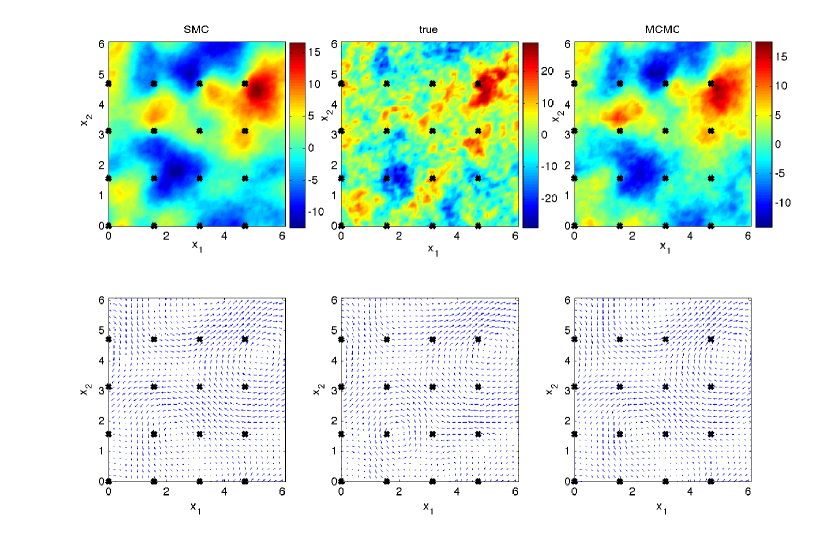
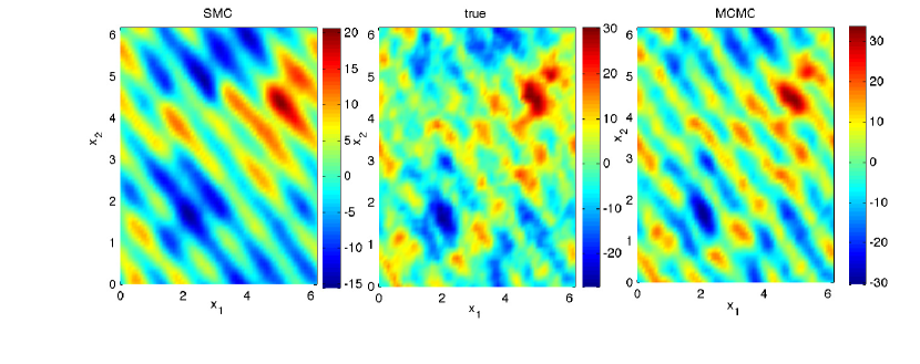
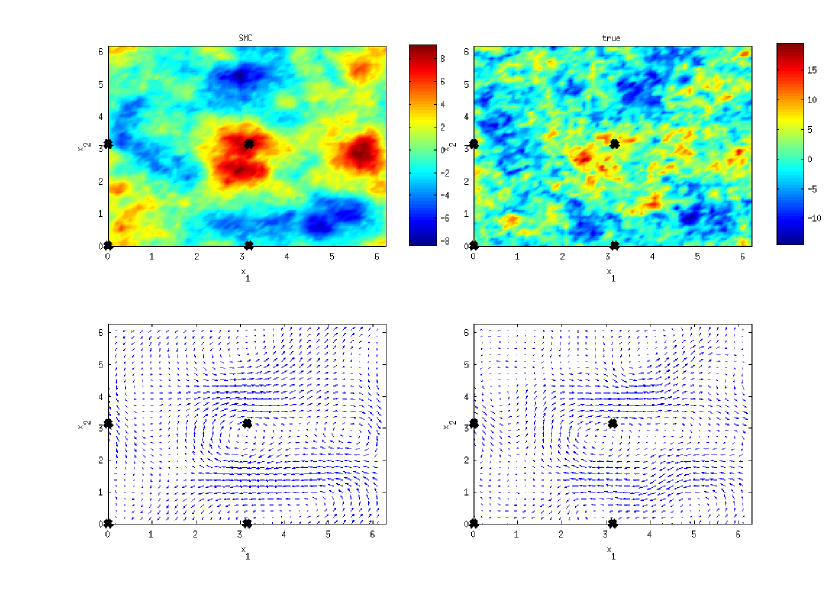
Figure 1 plots the posterior mean of the vorticity and velocity fields for the initial condition as estimated by our adaptive SMC algorithm (left) and the MCMC one (right). In the same plot the true field and its vorticity is displayed in the middle. The results from SMC and MCMC are very similar and both methods manage to capture the main features of the true field . The smoothing effect observed for the posterior means by both SMC and MCMC appears because the observations cannot provide substantial information about the high frequency Fourier coefficients. Figure 2 shows the posterior mean of the vorticity field this time for the terminal state instead of the initial condition (i.e. the push forward probability measure of under ).
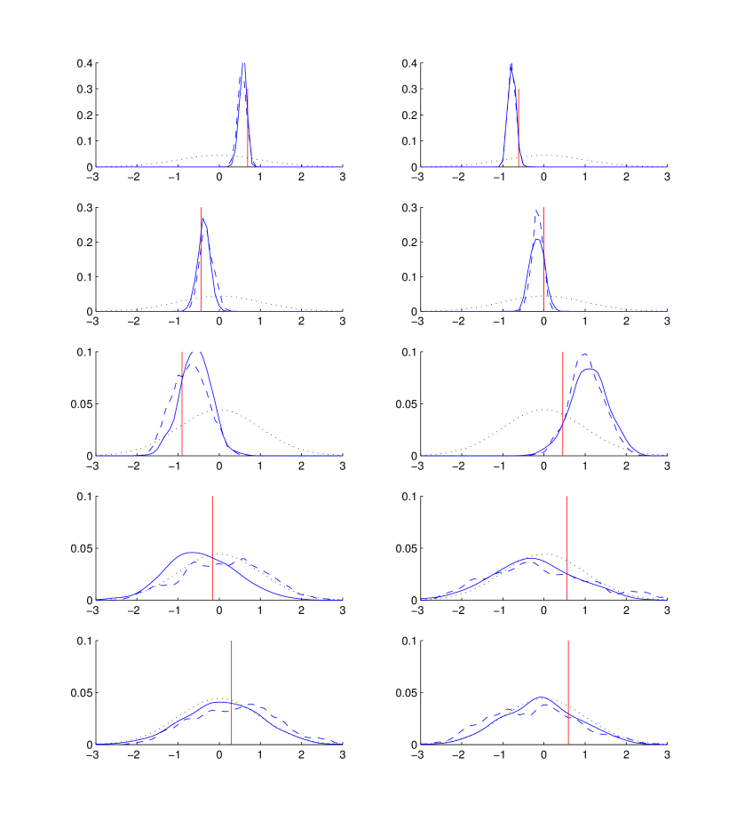
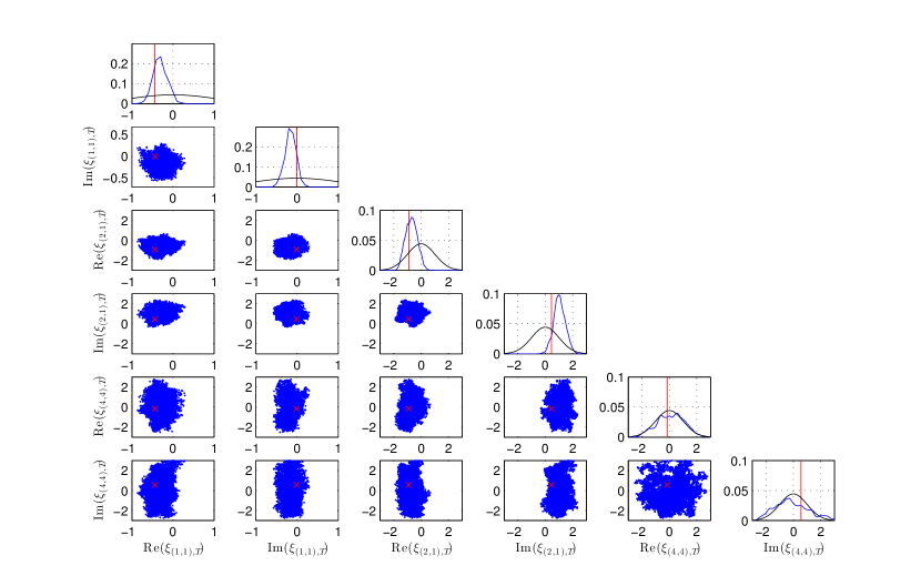
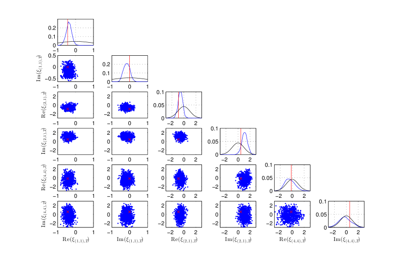
Note that the objective here is to approximate the full posterior and not just the mean. Figure 3 shows the estimated posterior density functions (PDFs) for a few (re-scaled) Fourier coefficients, (as defined in (9)), of different frequencies obtained using both SMC and MCMC. Recall the scaling in makes all prior densities equal to standard normals. In Figure 3 we plot the prior density (dotted), the posterior densities from SMC (solid) and MCMC (dashed) together with the true value of used for generating the data (vertical line). In Figures 4 and 6 we show scatter-plots over pairs of different frequencies from the (sub-sampled) MCMC trajectory and the SMC particles respectively. In all the aforementioned plots SMC and MCMC seem to be in close agreement, which provides numerical evidence that SMC samples correctly from the posterior distribution.
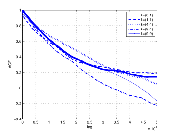
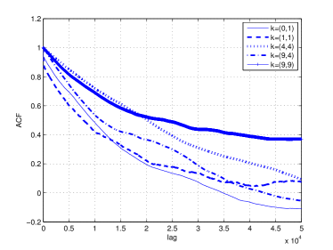
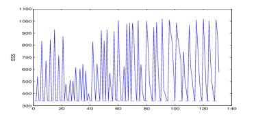
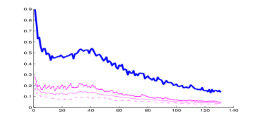
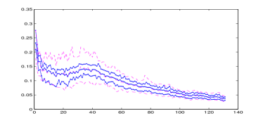
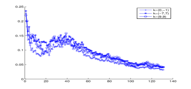
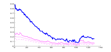
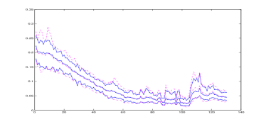
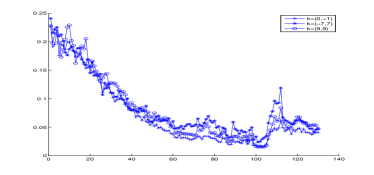
We proceed by presenting different measures of performance for MCMC and SMC. In Figure 5 we plot the autocorrelations of the MCMC trajectory for different Fourier coefficients. The mixing of the MCMC chain is quite slow, hence a large number of iterations was required for the MCMC approach to deliver reliable results. To monitor the performance of the SMC algorithm, Figure 7 includes plots of the ESS, the average acceptance ratio and the jittering indicator against each SMC iteration444By SMC iteration index we mean actually iteration , i.e. the number of times Steps 1-4 of Algorithm 4 have completed. Note is as in (11) and is a random variable determined by the algorithm.. Compared to the size of the data-set () the total number of extra tempering steps required here was about . In the bottom left plot in Figure 7 we observe how the average, maximum and minimum (over ) of changes with separately for when is within or outside the window of frequencies . For some indicative values of we also show in the lower right plot of Figure 7. does not seem to vary a lot with . It is certainly reassuring that all the MCMC steps seem to deliver considerable amount of jittering to all Fourier coefficients. Also, the amount of jittering appears to be fairly evenly spread over all Fourier coefficients, even if different MCMC proposals are used within and outside the window . Although supporting plots are not shown here, seemed to grow linearly with for every and each .
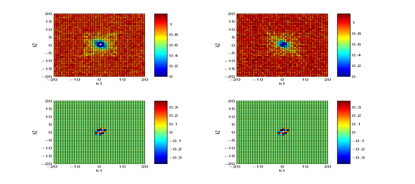
In Figure 8 we examine some statistical properties that are related to frequencies . In this plot, in the top row we use a heat map against to plot the ratio of estimated posterior marginal standard deviation for over the standard deviation of the (or the prior). The left plot corresponds to this ratio computed using the real parts of and the right plot to imaginary ones. In the bottom row we plot the posterior mean of against . We can deduce that the choice of treating high and low frequencies separately and adapting the MCMC steps only for a window of frequencies is reasonable, as most of the information in the data spreads over a number of frequencies covered by our chosen window .
5.2 Dataset B: Long-time Data-set with a Sparse Observation Grid
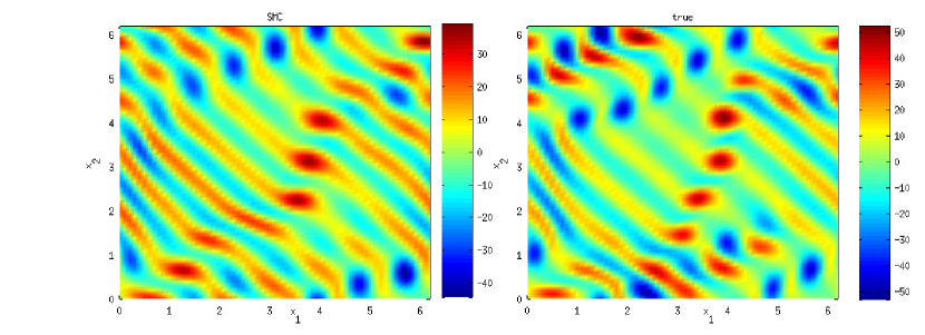
We will now present the results of the SMC method of Algorithm 4 when applied to Data-set B. This scenario is more challenging than the one with Data-set A, as we allow the Navier-Stokes dynamics to evolve for a longer period of time. We will follow a similar presentation as in the previous example. Figure 9 plots the posterior mean of the initial vorticity and velocity field. This plot can be used to compare the SMC estimates method versus the true values corresponding to . Although here we do not have a benchmark available like before, the smoothing effect in the estimates relative to the truth does not seem surprising based on the intuition gained from the previous example. In Figure 10 we show the posterior mean of the final vorticity together with the true one. Although few errors are present, the result is satisfying given the (mildly) chaotic nature of the forward dynamics.
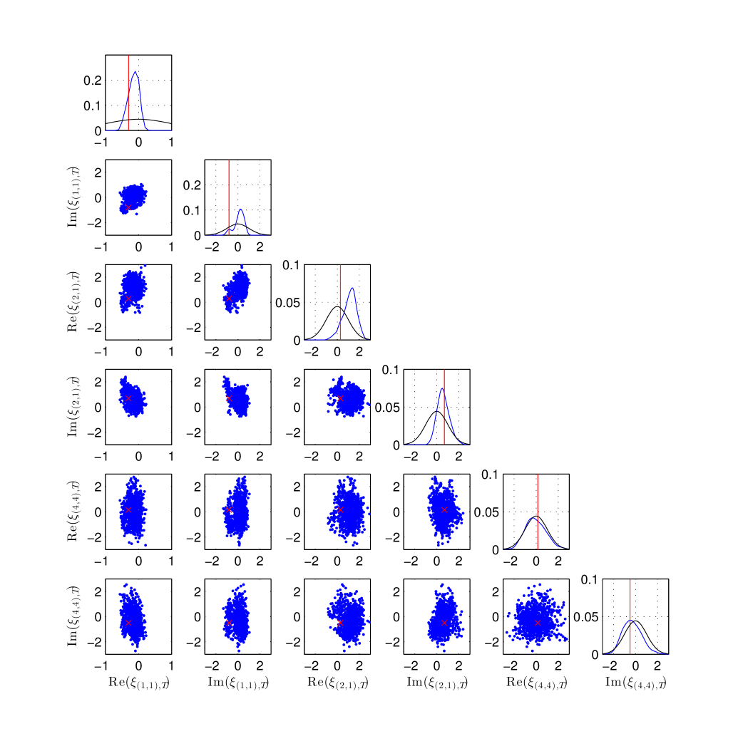
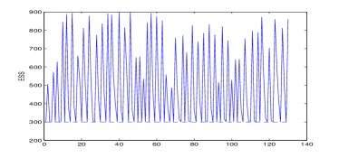
Figure 11 displays the approximate posterior densities of for a number of frequencies . The difference compared to Figure 3 for the previous example is that now we can see how changes for . As expected, each new block of observations contributes to shaping a more informative posterior. In Figure 12 we present the scatter-plots. To monitor the performance of SMC, in Figure 13 we plot the ESS, average acceptance ratio and all against as we did for the previous example. The algorithm uses almost the same number of tempering steps in total compared to the previous example. In addition, the acceptance ratio and stop decreasing after some iteration. We interpret this as a sign that stops changing fast with and that the particles form good approximations of the targeted sequence.
Finally, Figure 14 shows the heat maps against of the estimated posterior means of and the ratio of their marginal posterior standard deviations over their prior values, similarly to Figure 8 for Data-set A. Compared to the previous example the posterior seems to gain information from the observations for a wider window of low frequencies. Still, the choice of seems to be justified.
6 Discussion and Extensions
This paper aims to make a significant contribution towards challenging the perception that SMC is not useful for high-dimensional inverse problems. We believe this appears to be often the case when particle methods are implemented naively, see for example some negative results and exponential-in-dimension computational costs reported in Bengtsson et al. (2008); Snyder et al. (2008) for some cases involving stochastic dynamics. The added efficiency of our method compared to plain MCMC can be attributed to being able to employ a variety of adaptation steps that take advantage of the evolving particle population, hence tuning the algorithm effectively to the structure of the target distributions in the SMC sequence. SMC algorithms are also appealing to practitioners given the inherent ability to parallelize many steps in the algorithm thus drastically reducing execution times. As regards to understanding the effect of each block of observations, another useful aspect of the method is that the SMC sequence allows for monitoring the evolution of posterior distributions of interest as more observations arrive. In contrast, MCMC methods would require re-running the algorithm from scratch. In terms of the accuracy of the estimates we believe that SMC can be on a par with expensive MCMC methods, and this is illustrated clearly in the example with Data-set A.
We believe that the numerical results for the case study in this paper can motivate further investigations for using exact methods for data assimilation problems. In the present case study, the proposed SMC algorithm was able to provide results in an example (Data-set B) where the execution time of MCMC was prohibitive. Of course, PDE models used in practice can be much more complex that the Navier-Stokes equations used in this paper and might require a much finer resolution. Therefore, it would be unrealistic to claim that SMC methods can replace common heuristics. However, we believe that a thorough exploration of SMC methods in this context is beneficial for the data assimilation community, especially if they can be combined with some justifiable approximations to reduce the computational burden. Recent research initiatives in this direction include van Leeuwen (2010); Chorin et al. (2010); Rebeschini and van Handel (2013) when stochastic dynamics are used. In particular, Rebeschini and van Handel (2013) look at ways of reducing the intrinsic deficiency of importance sampling by avoiding to dismiss a whole high-dimensional particle when only few of its coordinates are in disagreement with the observation’s likelihood. It would be interesting to investigate how the methodology developed here can be combined with these aforementioned works.
-
•
At time execute Algorithm 4 for .
-
–
Store particles after resampling for all steps .
-
–
-
•
At times , execute Algorithm 4 with as follows:
-
1.
Replace in Algorithm 3 with an approximation of the posterior constructed using the particle population , e.g. , or some smooth Gaussian mixture centered at the particle locations .
-
2.
Store particles after resampling over all steps .
-
3.
Discard from memory particles .
-
1.
The work in this paper opens several paths for further investigations towards developing effective exact algorithms for data assimilation. In the context of high-dimensional Bayesian inference either for inverse problems or non-linear filtering we mention some possible extensions below:
- Gaussian
-
priors and beyond: We have chosen Gaussian priors with a fixed rate of decay for the eigenvalues of their covariance operators. In general, should be small enough so that posteriors for Fourier coefficients for which there is information in the data are not dominated by the prior, and this requires further empirical/theoretical investigations. Other prior distribution options could also be investigated. For instance, in the context of plain MCMC algorithms, the works in Cotter et al. (2013) and Dashti et al. (2011) have considered Sieve and Besov priors respectively.
- Algorithmic
-
design automation: The added flexibility of the SMC framework comes at the price of having to choose more algorithmic tuning parameters (in our context, choice of step-sizes , , window size , number of MCMC steps ). All these parameters are involved in the specification of the MCMC mutation step, that must provide enough jittering to the data. As explained in Section 4.4, there is a lot of information in the particle population that can be exploited towards a more ‘automated’ version of the algorithm presented here, with more (if not all) parameters determined on-the-fly.
- Algorithmic
-
robustness: We have considered the standardized squared jumping distance index in (22) as a way of measuring the diversity in the particles during the execution of the algorithm. In the case of Data-Set A, when an alternative algorithm (i.e. plain MCMC) is available for comparison, it appears that even small values () can suffice. More investigations are needed to determine what values of should one aim for in general.
- On-line
-
algorithms: The described algorithm has computational cost , so currently is not useful for on-line applications with very long data-sets. One possible remedy could be to use receding horizon estimation principles similar to Jazwinski (1968); Rawlings and Bakshi (2006) with a fixed lag or memory to reduce the computational cost to with increased memory requirements of . An example of such a procedure is shown in Algorithm 5, where one implements Algorithm 4 recursively with a fixed-lag approach and for the MCMC jittering steps in Algorithm 3 one uses instead of a Gaussian approximation (or a mixture of them) of the posterior at time . A bias will incur from using these approximations of the posterior at time in the subsequent mutations and importance sampling selections. Hopefully in some cases this bias might be small and uniform in time. In principle, one could also correct this estimation error using some form of importance sampling like Doucet et al. (2006), but it remains to be investigated whether this is possible to be implemented without requiring weight computations looking all the way back to and hence being impractical for long . Algorithm 5 bears some similarity with earlier works: in Stordal et al. (2011); Frei and Künsch (2012); Li (2012) the authors combine ensemble Kalman filtering or Gaussian mixtures with particle filters when the noise is present in the dynamics without any use of receding horizon or MCMC jittering steps and in Yang et al. (2010) the authors present a similar algorithm to Algorithm 5 intended for a computer vision application but again without using any MCMC mutation steps. We are currently investigating the performance and theoretical properties of Algorithm 5 when applied to inverse problems involving long observation sequences.
- Beyond
-
Navier-Stokes on a Torus: An advantage of the proposed SMC methodology is that it is generic and applicable to a wider class of applications than the particular Navier-Stokes inverse problem. One could use this method also with non-linear observations, different dynamical systems such as groundwater flow equations or other statistical inverse problems such as those examined in Stuart (2010); Cotter et al. (2013). In addition, a challenging extension could be to see how this work can be useful in the context of high dimensional filtering when noise is present in the dynamics.
Acknowledgements
The authors would like to thank Dan O. Crisan, Kody J.H. Law and Andrew M. Stuart for many useful discussions that provided valuable insight on the topic. We would also like to thank Vassilis Stathopoulos for his help on using Matlab(R) parallel jobs with MPI on the SunGrid(R) engine of CSML at UCL. N. Kantas and A. Beskos received funding by EPSRC under grant EP/J01365X/1, which is gratefully acknowledged. A. Jasra and A. Beskos acknowledge also support from MOE Singapore.
References
- Andrieu and Thoms [2008] Christophe Andrieu and Johannes Thoms. A tutorial on adaptive MCMC. Statistics and Computing, 18(4):343–373, 2008.
- Bengtsson et al. [2008] Thomas Bengtsson, Peter Bickel, and Bo Li. Curse-of-dimensionality revisited: Collapse of the particle filter in very large scale systems. Probability and statistics: Essays in honor of David A. Freedman, 2:316–334, 2008.
- Bennett [2002] Andrew F Bennett. Inverse modeling of the ocean and atmosphere. Cambridge University Press, 2002.
- Beskos et al. [2008] Alexandros Beskos, Gareth Roberts, Andrew Stuart, and Jochen Voss. MCMC methods for diffusion bridges. Stochastics and Dynamics, 8(03):319–350, 2008.
- Beskos et al. [2013a] Alexandros Beskos, Dan Crisan, and Ajay Jasra. On the stability of sequential Monte Carlo methods in high dimensions. Annals of Applied Probability, 2013a. to appear.
- Beskos et al. [2013b] Alexandros Beskos, Dan Crisan, Ajay Jasra, and Nick Whiteley. Error bounds and normalizing constants for sequential Monte Carlo in high dimensions. Advances in Applied Probability, 2013b. to appear.
- Beskos et al. [2013c] Alexandros Beskos, Ajay Jasra, and Alexandre H Thiéry. On the convergence of adaptive sequential Monte Carlo methods. arXiv preprint arXiv:1306.6462, 2013c.
- Chopin [2002] Nicolas Chopin. A sequential particle filter method for static models. Biometrika, 89(3):539–552, 2002.
- Chorin et al. [2010] Alexandre J Chorin, Matthias Morzfeld, and Xuemin Tu. Implicit particle filters for data assimilation. Communications in Applied Mathematics and Computational Science, 5:221–240, 2010.
- Cotter et al. [2009] Simon L Cotter, Masoumeh Dashti, James C. Robinson, and Andrew M Stuart. Bayesian inverse problems for functions and applications to fluid mechanics. Inverse Problems, 25(11):115008, 2009.
- Cotter et al. [2010] Simon L Cotter, Masoumeh Dashti, and Andrew M Stuart. Approximation of Bayesian inverse problems for PDEs. SIAM Journal on Numerical Analysis, 48(1):322–345, 2010.
- Cotter et al. [2013] Simon L Cotter, Gareth O Roberts, Andrew M Stuart, and David White. MCMC methods for functions: modifying old algorithms to make them faster. Statistical Science, 2013. to appear.
- Cox and Matthews [2002] Stephen M Cox and Paul C Matthews. Exponential time differencing for stiff systems. Journal of Computational Physics, 176(2):430–455, 2002.
- Da Prato and Zabczyk [2008] Guiseppe Da Prato and Jerzy Zabczyk. Stochastic equations in infinite dimensions. Cambridge University Press, 2008.
- Dashti et al. [2011] Masoumeh Dashti, Stephen Harris, and Andrew Stuart. Besov priors for Bayesian inverse problems. arXiv preprint arXiv:1105.0889, 2011.
- Del Moral [2004] Pierre Del Moral. Feynman-Kac Formulae. Springer, 2004.
- Del Moral et al. [2006] Pierre Del Moral, Arnaud Doucet, and Ajay Jasra. Sequential Monte Carlo samplers. Journal of the Royal Statistical Society: Series B (Statistical Methodology), 68(3):411–436, 2006.
- Doucet et al. [2001] Arnaud Doucet, Nando de Freitas, and Neil Gordon, editors. Sequential Monte Carlo methods in practice. Statistics for Engineering and Information Science. Springer-Verlag, New York, 2001.
- Doucet et al. [2006] Arnaud Doucet, Mark Briers, and Stéphane Sénécal. Efficient block sampling strategies for sequential Monte Carlo methods. Journal of Computational and Graphical Statistics, 15(3):693–711, 2006.
- Evensen [2009] Geir Evensen. Data assimilation: the ensemble Kalman filter. Springer, 2009.
- Foias et al. [2001] Ciprian Foias, Oscar Manley, Ricardo Rosa, and Roger Temam. Navier-Stokes equations and turbulence, volume 83. Cambridge University Press, 2001.
- Frei and Künsch [2012] Marco Frei and Hans R Künsch. Bridging the ensemble Kalman and particle filter. arXiv preprint arXiv:1208.0463, 2012.
- Gilks et al. [1996] W. R. Gilks, S. Richardson, and D. J. Spiegelhalter, editors. Markov chain Monte Carlo in practice. Interdisciplinary Statistics. Chapman & Hall, London, 1996.
- Giraud and Del Moral [2012] François Giraud and Pierre Del Moral. Non-asymptotic analysis of adaptive and annealed Feynman-Kac particle models. arXiv preprint arXiv:1209.5654, 2012.
- Hairer et al. [2011] Martin Hairer, Andrew Stuart, and Sebastian Vollmer. Spectral gaps for a Metropolis-Hastings algorithm in infinite dimensions. arXiv preprint arXiv:1112.1392, 2011.
- Hesthaven et al. [2007] Jan S Hesthaven, Sigal Gottlieb, and David Gottlieb. Spectral methods for time-dependent problems, volume 21. Cambridge University Press, 2007.
- Jasra et al. [2011] Ajay Jasra, David A Stephens, Arnaud Doucet, and Theodoros Tsagaris. Inference for Lévy-driven stochastic volatility models via adaptive sequential Monte Carlo. Scandinavian Journal of Statistics, 38(1):1–22, 2011.
- Jazwinski [1968] Andrew Jazwinski. Limited memory optimal filtering. IEEE Transactions on Automatic Control, 13(5):558–563, 1968.
- Kaipio and Somersalo [2005] Jari P Kaipio and Erkki Somersalo. Statistical and computational inverse problems, volume 160. Springer Science+ Business Media, 2005.
- Law [2012] Kody JH Law. Proposals which speed-up function space MCMC. arXiv preprint arXiv:1212.4767, 2012.
- Law and Stuart [2011] Kody JH Law and AM Stuart. Evaluating data assimilation algorithms. arXiv preprint arXiv:1107.4118, 2011.
- Le Dimet and Talagrand [1986] François-Xavier Le Dimet and Olivier Talagrand. Variational algorithms for analysis and assimilation of meteorological observations: theoretical aspects. Tellus A, 38(2):97–110, 1986.
- Le Gland et al. [2011] François Le Gland, Valérie Monbet, and Vu-Duc Tran. Large sample asymptotics for the ensemble Kalman filter. In Dan Crisan and Boris Rozovskii, editors, The Oxford handbook of nonlinear filtering, pages 598–634. Oxford University Press, Oxford, 2011.
- Lee et al. [2010] Anthony Lee, Christopher Yau, Michael B Giles, Arnaud Doucet, and Christopher C Holmes. On the utility of graphics cards to perform massively parallel simulation of advanced Monte Carlo methods. Journal of Computational and Graphical Statistics, 19(4):769–789, 2010.
- Li [2012] Kai Li. Generalised particle filters. PhD thesis, Imperial College London, 2012.
- Martin et al. [2012] James Martin, Lucas C Wilcox, Carsten Burstedde, and Omar Ghattas. A stochastic Newton MCMC method for large-scale statistical inverse problems with application to seismic inversion. SIAM Journal on Scientific Computing, 34(3):A1460–A1487, 2012.
- Murray et al. [2013] Lawrence M Murray, Anthony Lee, and Pierre E Jacob. Rethinking resampling in the particle filter on graphics processing units. arXiv preprint arXiv:1301.4019, 2013.
- Neal [1999] Radford M Neal. Regression and classification using Gaussian process priors. In JM Bernardo, JO Berger, AFM Smith, and AP Dawid, editors, Bayesian Statistics 6: Proceedings of the Sixth Valencia International Meeting, June 6-10, 1998, volume 6, pages 475–491. Oxford University Press, Oxford, 1999.
- Neal [2001] Radford M Neal. Annealed importance sampling. Statistics and Computing, 11(2):125–139, 2001.
- Rawlings and Bakshi [2006] James B Rawlings and Bhavik R Bakshi. Particle filtering and moving horizon estimation. Computers & chemical engineering, 30(10):1529–1541, 2006.
- Rebeschini and van Handel [2013] Patrick Rebeschini and Ramon van Handel. Can local particle filters beat the curse of dimensionality? arXiv preprint arXiv:1301.6585, 2013.
- Robinson [2001] James C Robinson. Infinite-dimensional dynamical systems: an introduction to dissipative parabolic PDEs and the theory of global attractors, volume 28. Cambridge University Press, 2001.
- Sasaki [1958] Yoshikazu Sasaki. An objective analysis based on the variational method. J. Meteor. Soc. Japan, 36(3):77–88, 1958.
- Schäfer and Chopin [2013] Christian Schäfer and Nicolas Chopin. Sequential monte carlo on large binary sampling spaces. Statistics and Computing, 23(2):163–184, 2013.
- Schweizer [2012] Nikolaus Schweizer. Non-asymptotic error bounds for sequential MCMC and stability of Feynman-Kac propagators. arXiv preprint arXiv:1204.2382, 2012.
- Snyder et al. [2008] Chris Snyder, Thomas Bengtsson, Peter Bickel, and Jeff Anderson. Obstacles to high-dimensional particle filtering. Monthly Weather Review, 136(12):4629–4640, 2008.
- Stordal et al. [2011] Andreas S Stordal, Hans A Karlsen, Geir Nævdal, Hans J Skaug, and Brice Vallès. Bridging the ensemble Kalman filter and particle filters: the adaptive gaussian mixture filter. Computational Geosciences, 15(2):293–305, 2011.
- Stuart [2010] Andrew M Stuart. Inverse problems: a Bayesian perspective. Acta Numerica, 19(1):451–559, 2010.
- Talagrand and Courtier [1987] Olivier Talagrand and Philippe Courtier. Variational assimilation of meteorological observations with the adjoint vorticity equation. I and II: Theory and numerical results. Quarterly Journal of the Royal Meteorological Society, 113(478):1311–1347, 1987.
- Uecker [2009] Hannes Uecker. A short ad hoc introduction to spectral methods for parabolic PDE and the Navier–Stokes equations. Summer School Modern Computational Science, Oldenburg 2009, pages 169–209, 2009.
- van Leeuwen [2010] Peter Jan van Leeuwen. Nonlinear data assimilation in geosciences: an extremely efficient particle filter. Quarterly Journal of the Royal Meteorological Society, 136(653):1991–1999, 2010.
- Whiteley [2012] Nick Whiteley. Sequential Monte Carlo samplers: error bounds and insensitivity to initial conditions. Stochastic Analysis and Applications, 30(5):774–798, 2012.
- Yang et al. [2010] Ehwa Yang, Moongu Jeon, and Vladimir Shin. Receding horizon estimation for hybrid particle filters and application for robust visual tracking. In Pattern Recognition (ICPR), 2010 20th International Conference on, pages 3508–3512. IEEE, 2010.
- Zhou et al. [2013] Yan Zhou, Adam M Johansen, and John AD Aston. Towards automatic model comparison: an adaptive sequential Monte Carlo approach. arXiv preprint arXiv:1303.3123, 2013.
