Efficient hybrid entanglement concentration for quantum communications

Abstract

We present two groups of practical entanglement concentration protocols (ECPs) for optical hybrid entangled state (HES). In the first group, it contains two ECPs and both ECPs do not need to know the initial coefficients of the less-entangled state. The second group contains three ECPs and they need to know the initial coefficients. It is shown that the yield of the entanglement concentration in the second group is greater than the first group. Moreover, some protocols are based on the linear optics and can be easily realized under current experiment condition. These protocols may be useful in current hybrid quantum communication.

I introduction

The distribution of entanglement over long-distances is essential for potential future application for quantum communication rmp ; book , such as teleportation teleportation , quantum key distribution(QKD) Ekert91 ; BBM92 ; QKD , quantum dense coding densecoding , quantum state sharing QSS1 ; QSS2 ; QSS3 ; QSSpra , and quantum secure direct communication long ; two-step ; lixhpra . But the quantum state transformation in quantum channel such as free space and optical fiber always suffers from the noise. The noise will make the photon loss and decoherence. It greatly limit the transmission distance in quantum communication. In order to overcome this flaw, the concept of the quantum repeater was introduced. In 1998, Briegel et al. proposed the quantum repeaters based on quantum purification and quantum swapping repeater1 ; repeater2 . The basic idea is to divide the whole long-distance channel into many short segments. The photons are transmitted between each segments, which is comparable to the channel attenuation length. In 2001, Duan et al. developed this idea and proposed a quantum repeater protocol based on the atomic ensembles and optical elements DLCZ . It is usually called the DLCZ protocol. Meanwhile, there are other groups focused on the quantum repeaters for both theory and experiments repeater3 ; repeater4 ; repeater5 ; repeater6 ; repeater7 ; repeater8 ; repeater9 ; repeater10 ; wangtiejun ; detail6 ; jiang ; Rydberg5 ; Rydberg6 ; repeaterRMP ; quantumnetworkrmp . Most current schemes focus on the heralded creation of very high fidelity base-level pairs based on the atomic ensembles and linear optics repeaterRMP .

On the other hand, another kind of quantum repeaters named hybrid quantum repeaters have been widely discussed hybid1 ; hybid2 ; hybid3 ; hybid4 ; hybid5 ; hybid6 ; hybid7 ; hybid8 ; hybid9 ; hybid10 ; hybid11 ; hybid12 ; hybrid13 ; hybridteleportation . Comparing with the previous quantum repeater protocols, the biggest difference is that in the stage of entanglement connection, they use the coherent state instead of the single photon, to create the hybrid entangled state (HES) as

$$|\Phi^{+}\rangle=\frac{1}{\sqrt{2}}(|\bar{0}\rangle|\beta\rangle+|\bar{1}\rangle|-\beta\rangle).$$ (1)

Here the $|\pm\beta\rangle$ is the coherent states, and $|\bar{0}\rangle$, $|\bar{1}\rangle$ are the single qubit. The single qubit may be the individual $\Lambda$-type atom, the trapped ion, a neutral donor impurity in semiconductors, the nitrogen-vacancy (NV) center in a diamond with a nuclear spin, a single electron trapped in quantum dots hybid1 ; hybid3 ; hybid12 , or a single photon encoded in the polarization which will make the HES become $\frac{1}{\sqrt{2}}(|H\rangle|\beta\rangle+|V\rangle|-\beta\rangle)$ hybridteleportation . $|H\rangle$ and $|V\rangle$ represent the horizonal and vertical polarization, respectively.

However, the imperfect operation on the single qubit and coherent state or the practical noise in the environment may make the maximally HES become a less-entangled state as

$$|\Phi_{\perp}^{+}\rangle=a|\bar{0}\rangle|\beta\rangle+b|\bar{1}\rangle|-\beta\rangle.$$ (2)

Here $|a|^{2}+|b|^{2}=1$. Unfortunately, the imperfect entangled state in Eq. (2) will make the fidelity of quantum teleportation degrade, the key in quantum cryptography insecure and quantum dense coding fail. Thus, before entanglement connection in hybrid quantum repeaters, one should recover the imperfect entangled states into the maximally ones shown in Eq. (1).

The entanglement concentration is a powerful way to recover such less-entangled states into maximally entangled states. It was proposed by Bennett et al. C.H.Bennett2 in 1996, which was called the Schmidt projection method. Later some groups showed that the quantum swapping can also be used to perform the entanglement concentration swapping1 ; swapping2 . Yamamoto et al. Yamamoto and Zhao et al. zhao1 proposed two similar protocols of the concentration with the linear optics, independently. Both protocols were demonstrated by experiments Yamamoto1 ; zhao2 . We call them PBS concentration protocol. The entanglement concentration protocols (ECPs) with cross-Kerr nonlinearity and solid system have also been proposed shengpra1 ; shengpra2 ; dengsingle ; wangchuan1 ; wangchuan2 ; wangchuan3 ; shengreview . Unfortunately, current ECPs cannot deal with the HES, for they focus on the discrete entangled photon pairs with the same degree of freedom C.H.Bennett2 ; swapping1 ; swapping2 ; Yamamoto ; zhao1 ; Yamamoto1 ; zhao2 ; shengpra1 .

In this paper, we will present two groups of ECPs for optical HES. In the first group, the parties do not need to know the initial coefficients of the less-entangled state. In the second group, they should know the initial coefficients. Interestingly, it is shown that if they know the initial coefficients, the total success probability in the second group is much greater than the first group. The HES in this paper is encoded in the single photon in polarization and the coherent state, for the optical HESs have been widely discussed recently hybridentanglement1 ; hybridentanglement2 ; hybridentanglement3 ; hybridentanglement4 ; hybridstate1 ; hybridstate2 ; hybridstate3 ; hybridstate5 ; hybridstate6 ; hybridstate8 . Especially, the HES of the form $\frac{1}{\sqrt{2}}(|H\rangle|\beta\rangle+|V\rangle|-\beta\rangle)$ can be generated in principle by performing a weak cross-Kerr nonlinear interaction between a single photon and a strong coherent state with the help of a displacement operation QND1 , and can be used to perform a scheme to realize deterministic quantum teleportation hybridteleportation . Certainly, the HES encoded in the other solid qubits and the coherent state can also be concentrated with the similar principle.

The first group contains two ECPs. In the first protocol, we use the polarization beam splitter (PBS) and beam splitter (BS) to perform a parity check, and then achieve the concentration task. We call it BS protocol. It is essentially inspired by the Schmidt projection method C.H.Bennett2 . The second protocol is an improvement of the first one for only one PBS is needed. We call it BS-improved protocol. The second group contains three ECPs. In the third protocol, we make a further improvement of the above ECPs. In each concentration step, we use only one pair of hybrid entangled pair and a single polarized photon, and it can reach the same success probability as the first one. We call it single-photon protocol. In the forth protocol, we resort to the quantum nondemolition (QND) constructed by cross-Kerr nonlinearity to improve the third protocol. We call it QND protocol. By repeating this QND protocol, the success probability can be greatly increased. Moreover, in the five ECP, we do not need any auxiliary photon and it can reach the same yield as the QND protocol by performing it only one time. Therefore, it is the optimal one. All protocols not only can be used to concentrate the partially single-photon and single-coherent state HES shown in Eq. (2), but also can be extended to deal with the cases of multi-particle and multi-coherent states.

This paper is organized as follows: In Sec. II, we explain the first and the second protocol, following the same principle of the conventional ECPs. In Sec. III, we describe our third protocol assisted with single photon. The Sec. IV is the forth protocol constructed by cross-Kerr nonlinearity. In Sec. V, we discuss the optimal ECP without any auxiliary photons. Finally, in Sec. VI, we make a discussion and conclusion.

II Conventional ECPs with linear optics

II.1 Conventional ECPs for single-photon and single-coherent hybrid entangled state

Fig. 1 is a schematic drawing of the basic principle of our ECP. Suppose Alice and Bob first share two copies of unknown HESs

$$|\Phi_{\perp}^{+}\rangle_{a1b1}=a|H\rangle_{a1}|\beta\rangle_{b1}+b|V\rangle_{a1}|-\beta\rangle_{b1},$$ (3)

and

$$|\Phi_{\perp}^{+}\rangle_{a2b2}=a|H\rangle_{a2}|\beta\rangle_{b2}+b|V\rangle_{a2}|-\beta\rangle_{b2}.$$ (4)

The single photons are shared by Alice and the coherent states are shared by Bob. The PBS in Alice’s location is to transmit the $|H\rangle$ polarized photon and reflect the $|V\rangle$ polarized photon. The 50:50 BS in Bob’s location is to make

$$|\beta\rangle_{b1}|\beta\rangle_{b2}\longrightarrow|\sqrt{2}\beta\rangle_{d1}|0\rangle_{d2},$$ (5)

$$|\beta\rangle_{b1}|-\beta\rangle_{b2}\longrightarrow|0\rangle_{d1}|\sqrt{2}\beta\rangle_{d2},$$ (6)

$$|-\beta\rangle_{b1}|\beta\rangle_{b2}\longrightarrow|0\rangle_{d1}|-\sqrt{2}\beta\rangle_{d2},$$ (7)

$$|-\beta\rangle_{b1}|-\beta\rangle_{b2}\longrightarrow|-\sqrt{2}\beta\rangle_{d1}|0\rangle_{d2}.$$ (8)

Here the $|0\rangle$ is the vacuum state. Alice first rotates her single photon in $a2$ spatial mode with $90^{\circ}$ by the half wave plate (HWP). The state $|\Phi_{\perp}^{+}\rangle_{a2b2}$ becomes

$$|\Phi_{\perp}^{+}\rangle^{\prime}_{a2b2}=a|V\rangle_{a2}|\beta\rangle_{b2}+b|H\rangle_{a2}|-\beta\rangle_{b2}.$$ (9)

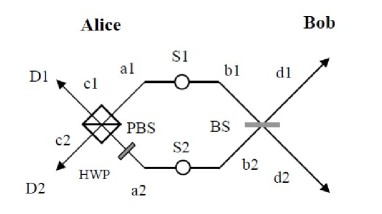
Figure 1: Schematic diagram of the proposed HES concentration. Two pairs of identical less-entangled HES are sent to Alice and Bob from sources S1 and S2, respectively. Alice receives the single photons, and the Bob receives the coherent states.

After the states passing though the PBS and BS, the initial system can be rewritten as

$$|\Phi_{\perp}^{+}\rangle_{a1b1}\otimes|\Phi_{\perp}^{+}\rangle^{\prime}_{a2b2}=(a|H\rangle_{a1}|\beta\rangle_{b1}+b|V\rangle_{a1}|-\beta\rangle_{b1})$$

$$\otimes(a|V\rangle_{a2}|\beta\rangle_{b2}+b|H\rangle_{a2}|-\beta\rangle_{b2})$$

$$=a^{2}|H\rangle_{a1}|V\rangle_{a2}|\beta\rangle_{b1}|\beta\rangle_{b2}$$

$$+b^{2}|V\rangle_{a1}|H\rangle_{a2}|-\beta\rangle_{b1}|-\beta\rangle_{b2}$$

$$+ab(|H\rangle_{a1}|H\rangle_{a2}|\beta\rangle_{b1}|-\beta\rangle_{b2}+|V\rangle_{a1}|V\rangle_{a2}$$

$$|-\beta\rangle_{b1}|\beta\rangle_{b2})\rightarrow a^{2}|H\rangle_{c2}|V\rangle_{c2}|\sqrt{2}\beta\rangle_{d1}|0\rangle_{d2}$$

$$+b^{2}|V\rangle_{c1}|H\rangle_{c1}|-\sqrt{2}\beta\rangle_{d1}|0\rangle_{d2}+ab(|H\rangle_{c1}|H\rangle_{c2}|0\rangle_{d1}$$

$$|\sqrt{2}\beta\rangle_{d2}+|V\rangle_{c1}|V\rangle_{c2}|0\rangle_{d1}|-\sqrt{2}\beta\rangle_{d2}).$$ (10)

From the above equation, the items $|H\rangle_{c2}|V\rangle_{c2}|\sqrt{2}\beta\rangle_{d1}|0\rangle_{d2}$ and $|V\rangle_{c1}|H\rangle_{c1}|-\sqrt{2}\beta\rangle_{d1}|0\rangle_{d2}$ will make two photons in the same output mode. But the other two items, $|H\rangle_{c1}|H\rangle_{c2}|0\rangle_{d1}|\sqrt{2}\beta\rangle_{d2}$ $|V\rangle_{c1}|V\rangle_{c2}|0\rangle_{d1}|-\sqrt{2}\beta\rangle_{d2}$ will make the outputs modes $c1$ and $c2$ both contain one photon. Therefore, by selecting only those events that there is exactly one photon at each output modes $c1$ and $c2$, Alice and Bob can project the above state into a maximally HES

$$|\Phi_{\perp}^{+}\rangle_{c} = \frac{1}{\sqrt{2}}(|H\rangle_{c1}|H\rangle_{c2}|0\rangle_{d1}|\sqrt{2}\beta\rangle_{d2}$$ (11)

$$+ |V\rangle_{c1}|V\rangle_{c2}|0\rangle_{d1}|-\sqrt{2}\beta\rangle_{d2})),$$

with a success probability of $2|ab|^{2}$. In order to generate a maximally entangled state between Alice and Bob, Alice should measure her photon in $c2$ mode in the basis $|\pm\rangle=\frac{1}{\sqrt{2}}(|H\rangle\pm|V\rangle)$. After performing these operations, if the measurement result is $|+\rangle$, it will leave the above state as

$$|\Phi_{\perp}^{+}\rangle^{\prime}_{ab}=\frac{1}{\sqrt{2}}(|H\rangle_{c1}|\sqrt{2}\beta\rangle_{d2}+|V\rangle_{c1}|-\sqrt{2}\beta\rangle_{d2}),$$ (12)

otherwise, it will leave the state as

$$|\Phi_{\perp}^{-}\rangle^{\prime}_{ab}=\frac{1}{\sqrt{2}}(|H\rangle_{c1}|\sqrt{2}\beta\rangle_{d2}-|V\rangle_{c1}|-\sqrt{2}\beta\rangle_{d2}).$$ (13)

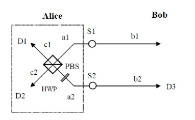
Figure 2: Schematic diagram of the improved HES concentration protocol. Comparing with Fig. 1, the BS is removed.

Both states are the maximally HESs. In order to get the same state of $|\Phi_{\perp}^{+}\rangle^{\prime}_{ab}$, Alice only needs to perform a simple local operation of phase rotation on her photon. It is interesting to compare above two states with Eq. (1). The obvious difference is that the amplitude of the coherent state is increased. It is quite different from the conventional ECPs. In fact, it is an obvious advantage of this protocol, for in a practical transmission, the coherent state always suffers from the noise, and the photon loss can not be avoided hybid1 ; hybid2 ; hybid3 ; hybid4 . The photon loss will decrease the amplitude of the coherent state, while in this protocol, after concentration, the amplitude has been increased automatically.

Actually, if they do not need to increase the amplitude of the coherent states, they can improve this ECP as shown in Fig. 2. Comparing with Fig. 1, they remove the BS, and make the whole system become

$$|\Phi_{\perp}^{+}\rangle_{a1b1}\otimes|\Phi_{\perp}^{+}\rangle^{\prime}_{a2b2}=(a|H\rangle_{a1}|\beta\rangle_{b1}+b|V\rangle_{a1}|-\beta\rangle_{b1})$$

$$\otimes(a|V\rangle_{a2}|\beta\rangle_{b2}+b|H\rangle_{a2}|-\beta\rangle_{b2})$$

$$=a^{2}|H\rangle_{a1}|V\rangle_{a2}|\beta\rangle_{b1}|\beta\rangle_{b2}$$

$$+b^{2}|V\rangle_{a1}|H\rangle_{a2}|-\beta\rangle_{b1}|-\beta\rangle_{b2}$$

$$+ab(|H\rangle_{a1}|H\rangle_{a2}|\beta\rangle_{b1}|-\beta\rangle_{b2}+|V\rangle_{a1}|V\rangle_{a2}$$

$$|-\beta\rangle_{b1}|\beta\rangle_{b2})\rightarrow a^{2}|H\rangle_{c2}|V\rangle_{c2}|\beta\rangle_{b1}|\beta\rangle_{b2}$$

$$+b^{2}|V\rangle_{c1}|H\rangle_{c1}|-\beta\rangle_{b1}|-\beta\rangle_{b2}$$

$$+ab(|H\rangle_{c1}|H\rangle_{c2}|\beta\rangle_{b1}|-\beta\rangle_{b2}+|V\rangle_{c1}|V\rangle_{c2}|-\beta\rangle_{b1}|\beta\rangle_{b2}).$$

Following the same principle, if the spatial modes $c1$ and $c2$ both contain one photon, above state becomes

$$|\Phi_{\perp}^{+}\rangle^{\prime}_{c} = \frac{1}{\sqrt{2}}(|H\rangle_{c1}|H\rangle_{c2}|\beta\rangle_{b1}|-\beta\rangle_{b2}$$ (14)

$$+ |V\rangle_{c1}|V\rangle_{c2}|-\beta\rangle_{b1}|\beta\rangle_{b2})),$$

with the success probability of $2|ab|^{2}$. In order to obtain the maximally entangled state, Alice measures the photon in the spatial mode $c2$ in the basis $|\pm\rangle$ and Bob measures the coherent state using the photon number detector $|n\rangle\langle n|$, which cannot distinguish the $|\pm\beta\rangle$. To realize the projection $|n\rangle\langle n|$ deterministically, one should use quantum nondemolition detection (QND) he1 ; lin1 . After performing these measurements, they can obtain

$$|\Phi_{\perp}^{+}\rangle^{\prime\prime}_{ab}=\frac{1}{\sqrt{2}}(|H\rangle_{c1}|\beta\rangle+|V\rangle|-\beta\rangle_{d2}),$$ (15)

if the Alice’s measurement result is $|+\rangle$. Otherwise, they will obtain

$$|\Phi_{\perp}^{-}\rangle^{\prime}_{ab}=\frac{1}{\sqrt{2}}(|H\rangle_{c1}|\beta\rangle-|V\rangle|-\beta\rangle_{d2}),$$ (16)

if the measurement result is $|-\rangle$. Both Eqs. (15) and (16) are the desired states. In order to obtain Eq. (15), Alice needs to perform a phase-flip operation on her photon.

The ECPs described in Fig. 1 and Fig. 2 are essentially followed the traditional ECPs, such as Refs.zhao1 ; Yamamoto . They should require two copies of less-entangled pairs, and do not need to know the initial coefficients of the states. However, the ECPs described in Fig. 1 and Fig. 2 are quite different. In Fig. 1, both the single photons and the coherent states should be operated. After the two single photons being in the different output modes, the two coherent states passing through BS will make the amplitude of coherent state increase. Though this ECP cannot obtain the desired maximally entangled state, the increased amplitude of the coherent state will make this ECP extremely useful in practical quantum communication because the photon loss. Certainly, if we only require to concentrate the less-entangled state, we can adopt the second ECP by removing the BS.

II.2 Conventional ECP for multi-photon and multi-coherent state

Furthermore, it is straightforward to extend these ECPs to concentrate the HES with multi-photon and multi-coherent state. In this section, we follow the principle of BS protocol to explain the ECP for multi-photon and multi-coherent state. The BS-improved protocol can also be used to concentrate the less-entangled state with multi-photon and multi-coherent state. For instance, the initial state is described as follows

$$|\Phi_{\perp}^{+}\rangle_{NM} = a|HH\cdots H\rangle_{N}|\beta\beta\cdots\beta\rangle_{M}$$ (17)

$$+ b|VV\cdots V\rangle_{N}|-\beta-\beta\cdots-\beta\rangle_{M}.$$

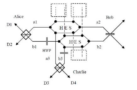
Figure 3: Schematic diagram of the ECP for multi-photon and multi-coherent state HES. Each parties will receive two single photons or two coherent states.

The $N$ is the number of the single photon, and $M$ is the number of the coherent state. In Fig. 3, two copies of such states are distributed to different parties, say Alice, Bob, Charlie, etc. The whole composite system can be rewritten as

$$|\Phi_{\perp}^{+}\rangle^{\prime}_{2N2M}=|\Phi_{\perp}^{+}\rangle_{NM}\otimes|\Phi_{\perp}^{+}\rangle_{NM}$$ (18)

$$= (a|H\rangle_{1}|H\rangle_{2}\cdots|H\rangle_{N}|\beta\rangle_{1}|\beta\rangle_{2}\cdots|\beta\rangle_{M}$$

$$+ b|V\rangle_{1}|V\rangle_{2}\cdots V\rangle_{N}|-\beta\rangle_{1}|-\beta\rangle_{2}\cdots|-\beta\rangle_{M})$$

$$\otimes a|H\rangle_{N+1}|H\rangle_{N+2}\cdots|H\rangle_{2N}|\beta\rangle_{M+1}|\beta\rangle_{M+2}\cdots|\beta\rangle_{2M}$$

$$+ b|V\rangle_{N+1}|V\rangle_{N+2}\cdots V\rangle_{2N}$$

$$|-\beta\rangle_{M+1}|-\beta\rangle_{M+2}\cdots|-\beta\rangle_{2M}).$$

Alice receives the photon 1 and photon $N+1$, Bob receives the coherent state $|\beta\rangle_{1}$ and $|\beta\rangle_{M+1}$, etc. Before performing the ECP, each parities who own the single photon first rotate the photons from number $N+1$ to $2N$ by $90^{\circ}$ similar to the case of above section. Therefore, the whole state becomes

$$|\Phi_{\perp}^{+}\rangle^{\prime\prime}_{2N2M}=|\Phi_{\perp}^{+}\rangle_{NM}\otimes|\Phi_{\perp}^{+}\rangle_{NM}$$ (19)

$$= (a|H\rangle_{1}|H\rangle_{2}\cdots|H\rangle_{N}|\beta\rangle_{1}|\beta\rangle_{2}\cdots|\beta\rangle_{M}$$

$$+ b|V\rangle_{1}|V\rangle_{2}\cdots V\rangle_{N}|-\beta\rangle_{1}|-\beta\rangle_{2}\cdots|-\beta\rangle_{M})$$

$$\otimes a|V\rangle_{N+1}|V\rangle_{N+2}\cdots|V\rangle_{2N}|\beta\rangle_{M+1}|\beta\rangle_{M+2}\cdots|\beta\rangle_{2M}$$

$$+ b|H\rangle_{N+1}|H\rangle_{N+2}\cdots H\rangle_{2N}$$

$$|-\beta\rangle_{M+1}|-\beta\rangle_{M+2}\cdots|-\beta\rangle_{2M}).$$

From Fig. 3, each single photon passes through the PBSs and each coherent state passes through the BSs. Finally, they choose the cases that each detector after PBS in Alice’s location exactly registers one photon, and they will get

$$|\Phi_{\perp}^{+}\rangle^{\prime\prime\prime}_{2N2M} = \frac{1}{2}(|H\rangle_{1}|H\rangle_{2}\cdots|H\rangle_{2N})|0\rangle_{1}|0\rangle_{2}\cdots|0\rangle_{M}$$

$$|\sqrt{2}\beta\rangle_{M+1}|\sqrt{2}\beta\rangle_{M+2}\cdots|\sqrt{2}\beta\rangle_{2M}$$

$$+ |V\rangle_{1}|V\rangle_{2}\cdots|V\rangle_{2N})|0\rangle_{1}|0\rangle_{2}\cdots|0\rangle_{M}$$

$$|-\sqrt{2}\beta\rangle_{M+1}|-\sqrt{2}\beta\rangle_{M+2}\cdots|-\sqrt{2}\beta\rangle_{2M},$$

with the probability of $2|ab|^{2}$. The above state is also the maximally entangled state. By measuring the photons from $N+1$ to $2N$ in $|\pm\rangle$ basis, the state of the composite system becomes

$$|\Phi_{\perp}^{+}\rangle^{\prime\prime\prime}_{2N2M}$$

$$=\frac{1}{2}[|H\rangle_{1}|H\rangle_{2}\cdots|H\rangle_{N}(\frac{1}{\sqrt{2}})^{\otimes N}(|H\rangle+|V\rangle)^{\otimes N}$$

$$|0\rangle_{1}|0\rangle_{2}\cdots|0\rangle_{M}|\sqrt{2}\beta\rangle_{M+1}|\sqrt{2}\beta\rangle_{M+2}\cdots|\sqrt{2}\beta\rangle_{2M}$$

$$+|V\rangle_{1}|V\rangle_{2}\cdots|V\rangle_{N}(\frac{1}{\sqrt{2}})^{\otimes N}(|H\rangle-|V\rangle)^{\otimes N}$$

$$|0\rangle_{1}|0\rangle_{2}\cdots|0\rangle_{M}$$

$$|-\sqrt{2}\beta\rangle_{M+1}|-\sqrt{2}\beta\rangle_{M+2}\cdots|-\sqrt{2}\beta\rangle_{2M}].$$ (21)

If the number of the single-photon outcome in $|V\rangle$ is even, they will get

$$|\Phi_{\perp}^{+}\rangle^{\prime\prime\prime}_{NM}=\frac{1}{\sqrt{2}}(|H\rangle_{1}|H\rangle_{2}\cdots|H\rangle_{N}$$

$$|\sqrt{2}\beta\rangle_{1}|\sqrt{2}\beta\rangle_{2}\cdots|\sqrt{2}\beta\rangle_{M}$$

$$+|V\rangle_{1}|V\rangle_{2}\cdots|V\rangle_{N}$$

$$|-\sqrt{2}\beta\rangle_{M}|-\sqrt{2}\beta\rangle_{M}\cdots|-\sqrt{2}\beta\rangle_{M}),$$ (22)

otherwise, they will get

$$|\Phi_{\perp}^{-}\rangle^{\prime\prime\prime}_{NM}=\frac{1}{\sqrt{2}}(|H\rangle_{1}|H\rangle_{2}\cdots|H\rangle_{N}$$

$$|\sqrt{2}\beta\rangle_{1}|\sqrt{2}\beta\rangle_{2}\cdots|\sqrt{2}\beta\rangle_{M}$$

$$-|V\rangle_{1}|V\rangle_{2}\cdots|V\rangle_{N}$$

$$|-\sqrt{2}\beta\rangle_{M}|-\sqrt{2}\beta\rangle_{M}\cdots|-\sqrt{2}\beta\rangle_{M}).$$ (23)

Both states in Eqs. (22) and (23) are the maximally entangled states. In order to obtain $|\Phi_{\perp}^{+}\rangle^{\prime\prime\prime}_{NM}$, they should perform a phase-flip operation on one of the single polarized photons to convert $|\Phi_{\perp}^{-}\rangle^{\prime\prime\prime}_{NM}$ to $|\Phi_{\perp}^{+}\rangle^{\prime\prime\prime}_{NM}$.

III Hybrid ECP assisted with single photon

In above section, we have explained two ECPs for HES. One of the advantages of such ECPs is that they do not need to know the exact coefficients of the initial less-entangled state, for they always select the same copies. It is not difficult for Alice and Bob to know the information about the parameters $a$ and $b$ if they can measure an enough number of sample photon pairs, during a practical quantum communication dengsingle . Actually, if the initial coefficients $a$ and $b$ is exactly known, above ECPs will be further simplified and improved. That is, they only need one single photon to complete the task. Inspirited by the Ref. shengpra2 , the basic principle of this improved ECP is shown in Fig. 4. The S1 emits the state similar to Eq. (3), and S2 emits a single photon of the form

$$|\Phi\rangle_{a2}=a|H\rangle_{a2}+b|V\rangle_{a2}.$$ (24)

Alice first rotates the $|\Phi\rangle_{a2}$ by HWP and makes it become

$$|\Phi\rangle_{a3}=a|V\rangle_{a3}+b|H\rangle_{a3}.$$ (25)

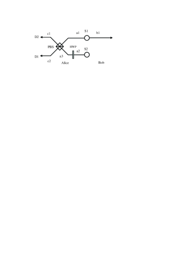
Figure 4: Schematic diagram of the concentration protocol assisted with single photons. Comparing with Fig. 1, the most difference is that the source of S2 emits a single photon. This figure is rather similar to Ref.shengpra2 . The difference is that the S1 emits the less-entangled HES.

Then the whole system $|\Phi_{\perp}^{+}\rangle_{a1b1}$ combined with $|\Phi\rangle_{a3}$ evolves as

$$|\Phi_{\perp}^{+}\rangle_{a1b1}\otimes|\Phi\rangle_{a3}$$

$$=(a|H\rangle_{a1}|\beta\rangle_{b1}+b|V\rangle_{a1}|-\beta\rangle_{b1})\otimes(a|V\rangle_{a3}+b|H\rangle_{a3})$$

$$=a^{2}|H\rangle_{a1}|V\rangle_{a3}|\beta\rangle_{b1}+b^{2}|V\rangle_{a1}|H\rangle_{a3}|-\beta\rangle_{b1}$$

$$+ab(|H\rangle_{a1}|H\rangle_{a3}|\beta\rangle_{b1}+|V\rangle_{a1}|V\rangle_{a3}|-\beta\rangle_{b1}).$$ (26)

After the PBS, it is easy to find that the items $|H\rangle|V\rangle|\beta\rangle$ and $|V\rangle|H\rangle|-\beta\rangle$ will make the two photons in the same output mode. Only $|H\rangle|H\rangle|\beta\rangle$ and $|V\rangle|V\rangle|-\beta\rangle$ make the both output modes contain one photon. By selecting the case that both spatial mode $c1$ and $c2$ containing one photon, the above state collapses to

$$|\Phi_{\bot}^{+}\rangle_{1}=\frac{1}{\sqrt{2}}(|H\rangle_{c1}|H\rangle_{c2}|\beta\rangle_{b1}+|V\rangle_{c1}|V\rangle_{c2}|-\beta\rangle_{b1}),$$ (27)

with the probability of $2|ab|^{2}$. Then Alice measures the photon in $c2$ mode in the basis $|\pm\rangle=\frac{1}{\sqrt{2}}(|H\rangle\pm|V\rangle)$. If the measurement result is $|+\rangle$, they will get

$$|\Phi_{\bot}^{+}\rangle^{\prime\prime}_{ab}=\frac{1}{\sqrt{2}}(|H\rangle_{c1}|\beta\rangle_{b1}+|V\rangle_{c1}|-\beta\rangle_{b1}),$$ (28)

otherwise, if the measurement result is $|-\rangle$, they will get

$$|\Phi_{\bot}^{-}\rangle^{\prime\prime}_{ab}=\frac{1}{\sqrt{2}}(|H\rangle_{c1}|\beta\rangle_{b1}-|V\rangle_{c1}|-\beta\rangle_{b1}).$$ (29)

Both states are the maximally HESs. In order to get the same state of $|\Phi_{\perp}^{+}\rangle^{\prime\prime}_{ab}$, Alice only performs a simple local operation of phase rotation on her photon.

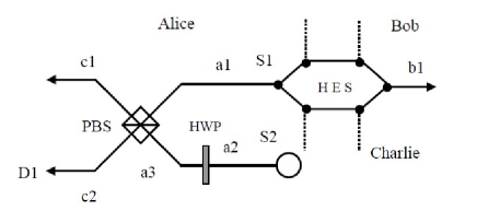
Figure 5: Schematic diagram of the concentration protocol for multi-photon and multi-coherent state, assisted with single photon. It is much simpler than Fig. 3, for each parties only receive a single photon or a coherent state.

It is straightforward to extend this protocol to the case of multi-photon and multi-coherent state. The basic principle is shown in Fig. 5. The source S1 still distributes the HES with the form of Eq. (17) to each parties. The source S2 prepares a single photon with the same form of Eq. (24). After performing a bit-flip on the Eq. (24), the whole system can be written as

$$|\Phi_{\perp}^{+}\rangle_{NM}\otimes|\Phi\rangle_{a3}=(a|H\rangle|H\cdots H\rangle_{N}|\beta\beta\cdots\beta\rangle_{M}$$

$$+b|V\rangle|V\cdots V\rangle_{N}|-\beta-\beta\cdots-\beta\rangle_{M})\otimes(a|V\rangle+b|H\rangle)$$

$$=a^{2}|H\rangle|HV\rangle|H\cdots H\rangle_{N+1}|\beta\beta\cdots\beta\rangle_{M}$$

$$+b^{2}|V\rangle|H\rangle|V\cdots V\rangle_{N+1}|-\beta-\beta\cdots-\beta\rangle_{M}$$

$$+ab(|H\rangle|H\cdots H\rangle_{N+1}|\beta\beta\cdots\beta\rangle_{M}$$

$$+|V\rangle|V\cdots V\rangle_{N+1}|-\beta-\beta\cdots-\beta\rangle_{M}).$$ (30)

In above equation, for simple, we omit the spatial modes $a1$, $a3$, $b1$ etc. After passing through the PBS, if the spatial mode $c1$ and $c2$ both contain one photon, the combined state in above equation will collapse to

$$|\Phi_{\perp}^{+}\rangle^{\prime}_{N+1M}=\frac{1}{\sqrt{2}}(|H\rangle|H\cdots H\rangle_{N+1}|\beta\beta\cdots\beta\rangle_{M}$$

$$+|V\rangle|V\cdots V\rangle_{N+1}|-\beta-\beta\cdots-\beta\rangle_{M}),$$ (31)

with the probability of $2|ab|^{2}$. Following the same principle, Alice measures his photon in $a3$ mode in the basis $|\pm\rangle$. If the measurement result is $|+\rangle$, they will get

$$|\Phi_{\perp}^{+}\rangle^{\prime}_{NM}=\frac{1}{\sqrt{2}}(|H\rangle|H\cdots H\rangle_{N}|\beta\beta\cdots\beta\rangle_{M}$$

$$+|V\rangle|V\cdots V\rangle_{N}|-\beta-\beta\cdots-\beta\rangle_{M}),$$ (32)

otherwise, they will get

$$|\Phi_{\perp}^{-}\rangle^{\prime}_{NM}=\frac{1}{\sqrt{2}}(|H\rangle|H\cdots H\rangle_{N}|\beta\beta\cdots\beta\rangle_{M}$$

$$+|V\rangle|V\cdots V\rangle_{N}|-\beta-\beta\cdots-\beta\rangle_{M}).$$ (33)

From above discussion, the ECP assisted with the single photon make the whole protocol rather simple. On one hand, in each concentration step, they only require one pair of less-entangled state and can reach the same success probability with the first one, so that ECP is more economical than the first one. On the other hand, in the conventional ECPs, both Alice and Bob need to operate or measure their photons. But in the improved ECP, Bob needs to do nothing but to remain or discard his photons according to the Alice’s measurement results. This feature is rather useful for concentrating the multi-photon and multi-coherent state. In the BS protocol, each parties who owns the coherent states should let his two coherent states pass though the BS, while in the BS-improved protocol, they should measure one of their coherent states using the photon number projection. Therefore, in the single-photon protocol, they can reduce the operation and make the whole concentration step simple.

IV Hybrid ECP with cross-Kerr nonlinearity

In Sec. III, we have described our ECP with linear optics. It is easy to realize it in current technology. However, it is not optimal. The total success probability is only $2|ab|^{2}$. On the other hand, it is based on the post-selection principle. That is to say, after concentration, the photon will be destroyed. In this section, we will adopt QND constructed by weak cross-Kerr nonlinearity to achieve this task QND1 ; QND2 . After performing the concentration, the success probability can be greatly increased by repeating this protocol.

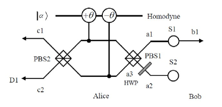
Figure 6: Schematic diagram of the ECP for HES with cross-Kerr nonlinearity.

From Fig. 6, the Hamiltonian of a cross-Kerr nonlinear medium can be written as $H=\hbar\chi\hat{n_{a}}\hat{n_{b}}$, where the $\hbar\chi$ is the coupling strength of the nonlinearity QND1 ; QND2 . It is decided by the material of cross-Kerr. Cross-Kerr nonlinearity has been widely studied in quantum information processing QND1 ; QND2 ; shengpra ; he1 ; lin1 ; shengpra1 ; qi ; dengsingle . The basis principle can be described as follows: if the coherent state $|\alpha\rangle$ combined with a quantum state $|\varphi\rangle$ couples with the cross-Kerr nonlinearity, the coherent state $|\alpha\rangle$ will pick up a phase shift. The phase shift is proportional to the photon number of the quantum state $|\varphi\rangle$. If the photon number of $|\varphi\rangle$ is $n$, the coherent state evolves to $|\alpha e^{in\theta}\rangle$. $\theta=\chi t$ and $t$ is the interaction time.

Now we reconsider the system $|\Phi_{\perp}^{+}\rangle_{a1b1}\otimes|\Phi\rangle_{a3}$ combined with the coherent state $|\alpha\rangle$

$$|\Phi_{\perp}^{+}\rangle_{a1b1}\otimes|\Phi\rangle_{a3}\otimes|\alpha\rangle$$

$$=(a|H\rangle_{a1}|\beta\rangle_{b1}+b|V\rangle_{a1}|-\beta\rangle_{b1})\otimes(a|V\rangle_{a3}+b|H\rangle_{a3})$$

$$\otimes|\alpha\rangle\rightarrow a^{2}|H\rangle_{a1}|V\rangle_{a3}|\beta\rangle_{b1}|\alpha e^{-i2\theta}\rangle$$

$$+b^{2}|V\rangle_{a1}|H\rangle_{a3}|-\beta\rangle_{b1}|\alpha e^{i2\theta}\rangle$$

$$+ab(|H\rangle_{a1}|H\rangle_{a3}|\beta\rangle_{b1}+|V\rangle_{a1}|V\rangle_{a3}|-\beta\rangle_{b1})|\alpha\rangle.$$ (34)

Obviously, if $|\alpha\rangle$ picks up no phase shift, the system will collapse to the state $|\Phi_{\bot}^{+}\rangle_{1}$, with the probability of $2|ab|^{2}$. It is the same as the case of using linear optics. Following the same principle described in Sec. III, after measuring the photon in $c2$ spatial mode in the basis $|\pm\rangle$, they will get $|\Phi_{\bot}^{+}\rangle^{\prime\prime}_{ab}$, if the measurement result is $|+\rangle$, or get $|\Phi_{\bot}^{-}\rangle^{\prime\prime}_{ab}$ if the measurement result is $|-\rangle$. However, there is another case that, if the $|\alpha\rangle$ picks up the phase shift $2\theta$. Here the homodyne measurement can make the $\pm 2\theta$ undistinguished. Then the remained state is

$$|\Phi_{\bot}^{+}\rangle^{\prime}_{1}=a^{2}|H\rangle_{a1}|V\rangle_{a3}|\beta\rangle_{b1}+b^{2}|V\rangle_{a1}|H\rangle_{a3}|-\beta\rangle_{b1}.$$ (35)

Then after measuring the photon in $a3$ spatial mode in $|\pm\rangle$, it becomes

$$|\Phi_{\bot}^{\pm}\rangle^{\prime\prime}_{1} = \frac{a^{2}}{\sqrt{|a|^{4}+|b|^{2}}}|H\rangle_{a1}|\beta\rangle_{b1}$$ (36)

$$\pm \frac{b^{2}}{\sqrt{|a|^{4}+|b|^{4}}}|V\rangle_{a1}|-\beta\rangle_{b1}.$$

Both $|\Phi_{\bot}^{\pm}\rangle^{\prime\prime}_{1}$ are less-entangled states, which can be reconcentrated in the next step. We take $|\Phi_{\bot}^{+}\rangle^{\prime\prime}_{1}$ for example. Source S2 emits another single photon with the form of

$$|\Phi\rangle^{\prime}_{a2}=\frac{a^{2}}{\sqrt{|a|^{4}+|b|^{4}}}|H\rangle_{a2}+\frac{b^{4}}{\sqrt{|a|^{4}+|b|^{4}}}|V\rangle_{a2}.$$ (37)

After a bit-flip operation, it becomes

$$|\Phi\rangle^{\prime}_{a3}=\frac{a^{2}}{\sqrt{|a|^{4}+|b|^{4}}}|V\rangle_{a3}+\frac{b^{4}}{\sqrt{|a|^{4}+|b|^{4}}}|H\rangle_{a3}.$$ (38)

Then the $|\Phi_{\bot}^{+}\rangle^{\prime\prime}_{1}\otimes|\Phi\rangle^{\prime}_{a3}$ combined with the $|\alpha\rangle$ evolves as

$$|\Phi_{\bot}^{+}\rangle^{\prime\prime}_{1}\otimes|\Phi\rangle^{\prime}_{a3}\otimes|\alpha\rangle=(\frac{a^{2}}{\sqrt{|a|^{4}+|b|^{4}}}|H\rangle_{a1}|\beta\rangle_{b1}$$

$$+\frac{b^{2}}{\sqrt{|a|^{4}+|b|^{4}}}|V\rangle_{a1}|-\beta\rangle_{b1})$$

$$\otimes(\frac{a^{2}}{\sqrt{|a|^{4}+|b|^{4}}}|V\rangle_{a3}+\frac{b^{2}}{\sqrt{|a|^{4}+|b|^{4}}}|H\rangle_{a3})\otimes|\alpha\rangle$$

$$\rightarrow\frac{a^{4}}{|a|^{4}+|b|^{4}}|H\rangle_{a1}|V\rangle_{a3}|\beta\rangle_{b1}|\alpha e^{-i2\theta}\rangle$$

$$+\frac{b^{4}}{|a|^{4}+|b|^{4}}|V\rangle_{a1}|H\rangle_{a3}|-\beta\rangle_{b1}|\alpha e^{i2\theta}\rangle$$

$$+\frac{a^{2}b^{2}}{|a|^{4}+|b|^{4}}(|H\rangle_{a1}|H\rangle_{a3}|\beta\rangle_{b1}+|V\rangle_{a1}|V\rangle_{a3}|-\beta\rangle_{b1})|\alpha\rangle.$$

Similarly, if $|\alpha\rangle$ picks up no phase shift, the above state can also collapse to the maximally entangled state with the form of $|\Phi_{\perp}^{+}\rangle_{1}$, with the success probability of $\frac{2|ab|^{4}}{|a|^{4}+|b|^{4}}$. The remained state can also be used to perform further concentration in the next step. It has the same success probability as the protocol in Ref. shengpra1 . In addition, it can also be extended to the case of multi-partite and multi-coherent HES. Briefly speaking, after the multi-photon and multi-coherent state distributed to each parities, one needs to substitute the PBS in Fig. 4 to the QND in Fig. 6, in Alice’s location.

V Hybrid ECP without any auxiliary photons

Recently, the group of Deng present a practical hyperentanglement concentration for two-photon four-qubit systems with linear optics hyperconcentration . In their protocol, it is shown that the arbitrary two-photon less-entangled state can be concentrated without any assisted photons, if they know exact coefficients of the initial state. Interestingly, their excellent idea is suitable for this hybrid ECP. Here we call it VBS protocol. The VBS is the variable beam splitter with the reflection coefficient $R=a/b$. As shown in Fig. 7, suppose that the Alice receive the single photon and Bob receive the coherent state. Suppose they know the coefficients $a$ and $b$, with $b>a$ and $|a|^{2}+|b|^{2}=1$. Therefore, after the state passing through the PBS1, VBS, and PBS2, it evolves as

$$|\Phi_{\perp}^{+}\rangle_{a1b1} = a|H\rangle_{a1}|\beta\rangle_{b1}+b|V\rangle_{a1}|-\beta\rangle_{b1}$$ (40)

$$\rightarrow a|H\rangle_{a1}|\beta\rangle_{b1}+b|V\rangle_{c1}|-\beta\rangle_{b1}$$

$$\rightarrow a|H\rangle_{a1}|\beta\rangle_{b1}+a|V\rangle_{c2}|-\beta\rangle_{b1}$$

$$+ \sqrt{|b|^{2}-|a|^{2}}|V\rangle_{c3}|-\beta\rangle_{b1}$$

$$\rightarrow a(|H\rangle_{a3}|\beta\rangle_{b1}+a|V\rangle_{a3}|-\beta\rangle_{b1})$$

$$+ \sqrt{|b|^{2}-|a|^{2}}|V\rangle_{c3}|-\beta\rangle_{b1}.$$

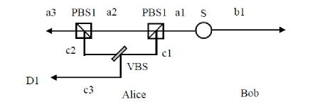
Figure 7: Schematic diagram of the ECP without any auxiliary photons.

From Eq. (40), if the single photon detector D1 detects the single photon, above state will collapse to the term $|V\rangle_{c3}|-\beta\rangle_{b1}$. On the other hand, if the single photon detector does not click any photon, the above state will collapse to the maximally entangled state with the success probability $2|a|^{2}$. Certainly, if $|a|>|b|$, this ECP can also work by adding the HWP in the spatial mode $a1$.

VI discussion and summary

By far, we have fully described our hybrid ECPs. It is interesting to compare these protocols with the conventional ECPs zhao1 ; Yamamoto1 . In BS protocol, it is essential to follow the similar idea as the conventional ones. In each step, one has to choose two copies of less-entangled pairs. After performing the protocol, at least one pair can be remained. The PBS is used to perform the parity check for the single photons and the BS acts the same role as the PBS, but for coherent states. After picking up the even parity states, the BS will make one output mode contain no photons. In another output mode, the amplitude of the coherent state has been increased. The increased coherent state become a great advantage because of the photon loss during the transmission. In single-photon protocol, we use the single photon to concentrate the HES, and reach the same success probability with the BS protocol. This protocol is rather simple. Only one PBS and two conventional detectors are required. Moreover, in each step, we only need one pair of less-entangled pair but can reach the same success probability as the BS protocol, which is more commercial than BS protocol. In addition, only one parties say Alice needs to operate this protocol. This feature makes it more powerful if consider the case of multi-photon and multi-coherent state. In BS protocol, each of parties should perform the parity check using PBS or BS. After that, they should exchange their measurement results to judge the whole process whether it is a success or failure by classical communication. Interestingly, in single-photon protocol, after Alice performing the parity check, she will ask other parties to remain or discard their photons. That is to say, here only one-way classical communication is required. The QND protocol is an improvement of the single-photon protocol. By introducing the QND to substitute the PBS, the whole protocol can be repeated to get a higher success probability. After successfully performing the ECP, the maximally HES can be remained to perform further application. In the last ECP, the whole ECP does not require any auxiliary photon, and can reach the same success probability as the QND protocol with only linear optics. We can calculate the yield of the maximally entangled state obtained in each protocols. We denote the yield as

$$Y_{1}=\frac{N_{c}}{N_{b}}.$$ (41)

Here $N_{b}$ is the number of originally less-entangled pairs and $N_{c}$ is the number of maximally entangled pairs after concentration. Obviously, in BS protocol and BS-improved protocol, they are

$$Y_{1}=|ab|^{2},$$ (42)

while in single-photon protocol, it is equal to

$$Y^{\prime}_{1}=2|ab|^{2}.$$ (43)

In QND protocol, we can get

$$Y^{\prime\prime}_{1} = 2|ab|^{2},$$

$$Y^{\prime\prime}_{2} = (1-2|ab|^{2})(\frac{2|ab|^{4}}{(|a|^{4}+|b|^{4})^{2}})=\frac{2|ab|^{4}}{|a|^{4}+|b|^{4}}$$

$$\cdots$$

$$Y^{\prime\prime}_{K} = \frac{2|ab|^{2^{K}}}{(|a|^{4}+|b|^{4})(|a|^{8}+|b|^{8})\cdots(|a|^{2^{N}}+|b|^{2^{K}})}$$ (44)

$$= \prod^{\infty}_{K=1}\frac{2|ab|^{2^{K}}}{(|a|^{2^{K}}+|b|^{2^{K}})}$$

The $K$ is the iteration number of this protocol. The total yield can be described as

$$Y^{\prime\prime}=Y^{\prime\prime}_{1}+Y^{\prime\prime}_{1}+\cdots+Y^{\prime\prime}_{K}=\sum^{\infty}_{K=1}Y^{\prime\prime}_{K}.$$ (45)

If the original state is the maximally entangled state with $a=b=\frac{1}{\sqrt{2}}$, we can get $Y_{1}=0.25$, $Y^{\prime}_{1}=0.5$, and $Y^{\prime\prime}=\frac{1}{2}+\frac{1}{4}+\cdots+\frac{1}{2^{K}}+\cdots=1$.

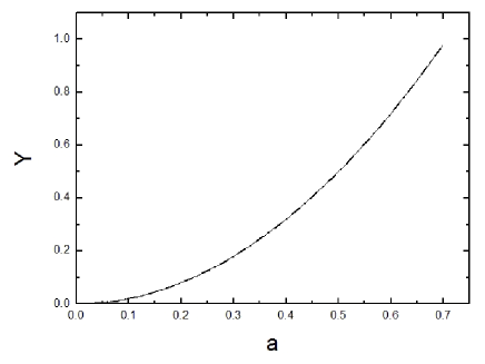
Figure 8: The total entanglement yield $Y$ of getting a maximally HES after the concentration protocol being operated for K times in QND protocol. For numerical simulation, we choose $K=10$. It can be seen that the value of $Y$ largely depends on the initial coefficient $a$. When $a=\frac{1}{\sqrt{2}}$, $Y$ can reaches the maximum as 1.

We both calculated the entanglement yield in the QND protocol and VBS protocol in Fig. 8. It is shown that the yield largely depends on the initial coefficient $a$. The yield $Y^{\prime}_{1}$ in single-photon protocol is essentially the case of $K=1$ in QND protocol. Interestingly, from Fig. 8, we only have one curve. Because by repeating the QND protocol for ten times, the yield is consist with the VBS protocol. Therefore, it is shown that the VBS protocol is the optimal one. Actually, the initial idea in this ECP is first proposed by the group of Deng hyperconcentration . The concentration step seems to be similar with Ref. hyperconcentration for we only need to operate the single polarized photon. Therefore, this ECP can also be extended to deal with the less-entangled state with multi-photon and multi-coherent state. Only one of the parties who own the single particle needs to operate the protocol.

Finally, let us discuss some further realization in experiment. In BS protocol, single-photon protocol and VBS protocol, we both resort to the linear optics, which is feasible in current technology. In QND protocol, we use the cross-Kerr nonlinearity to implement the QND. Though cross-Kerr nonlinearity has been widely studied in quantum information processes, we should acknowledge that it still has much controversy. The main reason is that the largest natural cross-Kerr nonlinearities are extremely weak ($\chi^{3}\approx 10^{-22}m^{2}V^{-2}$) kok1 . As mentioned by Gea-Banacloche, large shifts via the giant Kerr effect with single-photon wave packet is impossible in current technology Gea . Shapiro and Razavi also had the same results with Gea-BanaclocheShapiro1 ; Shapiro2 . However, Hofmann pointed out that a large phase-shift of $\pi$ can be achieved, with a single two-level atom in a one-side cavity hofmann . Fortunately, this protocol only works for a small value of the cross-Kerr nonlinearity and it greatly decrease the experimental difficulty. Actually, there are a great number of works which focuses on constructing the similar function of the QND for the photon-photon nonlinear interaction, such as these based on quantum dot spins in microwave cavity cavity1 ; cavity2 , a cavity waveguide cavity waveguide , hollow-core waveguides hollow-core waveguides , a Rydberg atom ensemble rydberg , and so on.

In summary, we have presented five different ECPs for HES. All protocols can be used to achieve the tasks of entanglement concentration. The second protocol can be seen as the improvement of the first one and the third protocol can also be regarded as the improvement of the first and the second protocol. These protocols have several advantages: in the first protocol, it is based on the simple optical elements, which can be realized in current experiment. It does not need to know the exact coefficients of the initial states. The second protocol is also based on the linear optics and it is much simpler than the first one. In the third protocol, it only needs one pair of less-entangled state, but can reach the same success probability as the first one. Moreover, in the fourth protocol, the concentrated states can be remained for further applications, by resorting to the QND. In addition, this ECP can be repeated to get a higher success probability. The last ECP is the optimal one. By performing this ECP for one time, it can reach the success probability $2|a|^{2}$. Moreover, it based on the linear optics which makes it feasible in current experiment condition. All advantages will make these ECPs useful in current long-distance quantum communications.

References

- (1) N. Gisin, G. Ribordy, W. Tittel, and H. Zbinden, Rev. Mod. Phys. 74, 145 (2002).
- (2) M. A. Nielsen and I. L. Chuang, Quantum Computation and Quantum Information (Cambridge University Press, Cambridge, England, 2000).
- (3) C. H. Bennett, G. Brassard, C. Crpeau, R. Jozsa, A. Peres, and W. K. Wootters, Phys. Rev. Lett. 70, 1895 (1993).
- (4) A. K. Ekert, Phys. Rev. Lett. 67, 661 (1991).
- (5) C. H. Bennett, G. Brassard, and N. D. Mermin, Phys. Rev. Lett. 68, 557 (1992).
- (6) J. L. Duligall, M. S. Godfrey, K. A. Harrison, W. J. Munro, and J. G. Rarity, New J. Phys. 8, 249 (2006).
- (7) C. H. Bennett and S. J. Wiesner, Phys. Rev. Lett. 69, 2881 (1992).
- (8) A. Karlsson, M. Koashi, and N. Imoto, Phys. Rev. A 59 162 (1999).
- (9) M Hillery, V.Bužek, and A. Berthiaume, Phys. Rev. A 59, 1829 (1999).
- (10) L. Xiao, G. L. Long, F. G. Deng and J. W. Pan, Phys. Rev. A 69, 052307 (2004).
- (11) F. G. Deng, X. H. Li, C. Y. Li, P. Zhou, and H. Y. Zhou, Phys. Rev. A 72, 044301 (2005).
- (12) G. L. Long and X. S. Liu, Phys. Rev. A 65, 032302 (2002).
- (13) F. G. Deng, G. L. Long, and X. S. Liu, Phys. Rev. A 68, 042317 (2003).
- (14) X. H. Li, F. G. Deng, and H. Y. Zhou, Phys. Rev. A 74, 054302 (2006).
- (15) H. J. Briegel, W. Dür, J. I. Cirac, and P. Zoller, Phys. Rev. Lett. 81, 5932 (1998).
- (16) W. Dür, H. J. Briegel, J. I. Cirac, and P. Zoller, Phys. Rev. A 59, 169 (1998).
- (17) L. M. Duan, M. D. Lukin, J. T. Cirac, and P. Zoller, Nature 414, 413 (2001).
- (18) A. Kuzmich, W. P. Bowen, A. D. Boozer, A. Boca, C. W. Chou, L. M. Duan and H. K. Kimble, Nature 423, 731 (2003).
- (19) C. H. Chou, J. Laurat, H. Deng, K. S. Choi, H. de Riedmatten, D. Felinto, and H. J Kimble, Science 316, 1316(2007).
- (20) C. Simon, H. de Riedmatten, M. Afzelius, N. Sangouard, H. Zbinden, and N. Gisin, Phys. Rev. Lett. 98, 190503 (2007).
- (21) B. Zhao, Z. B. Chen, Y. A. Chen, J. Schmiedmayer, and J. W. Pan, Phys. Rev. Lett. 98, 240502 (2007).
- (22) Z. B. Chen, B. Zhao, Y. A. CHen, J. Schmiedmayer, and J. W. Pan, phys. Rev. A 76, 022329(2007).
- (23) L. Jiang, J. M. Taylor, and M. D. Lukin, Phys. Rev. A 76, 012301(2007).
- (24) B. Zhao, M. Müller, K. Hammerer, and P. Zoller, Phys. Rev. A 81, 052329 (2010).
- (25) Y. Han, B. He, K. Heshami, C. Z. Li, and C. Simon, Phys. Rev. A 81, 052311 (2010).
- (26) O. A. Collins, S. D. Jenkins, A. Kuzmich, and T. A. B. Kennedy, Phys. Rev. Lett. 98, 060502 (2007).
- (27) N. Sangouard, C. Simon, B. Zhao, Y. A. Chen, H. de Riedmatten, J. W. Pan, and Gisin, Phys. Rev. A 77, 062301 (2008).
- (28) M. Afzelius, C. Simon, H. de Riedmatten, and N. Gisin, Phys. Rev. A 79, 052329 (2009).
- (29) H. de Riematten, M. Afzelius, M. U. Staudt, C. Simon, and N. Gisin, Nature 456, 773 (2008).
- (30) T. J. Wang, S. Y. Song, and G. L. Long, Phys. Rev. A 85, 062311 (2012).
- (31) L. M. Duan, and C. Monroe, Rev. Mod. Phys. 82, 1829 (2011).
- (32) N. Sangouard, C. Simon, H. de Riedmatten, and N. Gisin, Rev. Mod. Phys. 83, 33 (2011).
- (33) P. van Loock, T. D. Ladd, K. Sanaka, F. Yamaguchi, K. Nemoto, W. J. Munro, and Y. Yamamoto, Phys. Rev. Lett. 96, 240501 (2006).
- (34) W. J. Munro, R. Van Meter, S. G. R. Louis, and K. Nemoto, Phys. Rev. Lett. 101, 040502 (2008).
- (35) T. D. Ladd, P van Loock, K. Nemoto, W. J. Munro, and Y. Yamamoto, N. J. Phys. 8, 184 (2006).
- (36) T. P. Spiller, K. Nemoto, S. L. Braunstein, W. J. Munro, P van. Loock, and G. J. Milburn, N. J. Phys. 8, 30 (2006).
- (37) P. van Loock, N. Lütkenhaus, W. J. Munro, and K. Nemoto, Phys. Rev. A 78, 062319 (2008).
- (38) S. G. R. Louis, W. J. Munro, T. P. Spiller, and K. Nemoto, Phys. Rev. A 78, 022326(2008).
- (39) P van Loock, W. J. Munro, K. Nemoto, T. P. Spiller, T. D. Ladd, S. L. Braunstein, and G. J. Miburn, Phys. Rev. A 78, 022303(2008).
- (40) K. Azuma, N. Sota, R. Namiki, S. K. Özdemir, T. Yamamoto, M. Koashi, and N. Imoto, Phys. Rev. A 80, 060303(R) (2009).
- (41) W. J. Munro, K. A. Harrison, A. M. Stephens, S. J. Devitt, and K. Nemoto, Nature Photonics 4, 792 (2010).
- (42) K. Azuma, N. Sota, M. Koashi, and N. Imoto, Phys. Rev. A 81, 022325 (2010).
- (43) J. B. Brask, I. Rigas, E. S. Polzik, U. L. Andersen, and A. S. Srensen, Phys. Rev. Lett. 105, 160501 (2010).
- (44) K. Azuma, H. Takeda, M. Koashi, and N. Imoto, Phys. Rev. A 85 062309 (2012).
- (45) K. Azuma, and G. Kato, Phys. Rev. A 85, 060303(R) (2012).
- (46) S. W. Lee, and H. Jeong, Phys. Rev. A 87 022326 (2013).
- (47) C. H. Bennett, H. J. Bernstein, S. Popescu, and B. Schumacher, Phys. Rev. A 53, 2046 (1996).
- (48) S. Bose, V. Vedral, and P. L. Knight, Phys. Rev A 60, 194 (1999).
- (49) B. S. Shi, Y. K. Jiang, and G. C. Guo, Phys. Rev. A 62, 054301 (2000).
- (50) T. Yamamoto, M. Koashi, and N. Imoto, Phys. Rev. A 64, 012304 (2001).
- (51) Z. Zhao, J. W. Pan, and M. S. Zhan, Phys. Rev. A 64, 014301 (2001).
- (52) T. Yamamoto, M. Koashi, Ş. K. Özdemir, and N. Imoto Nature 421, 343 (2003).
- (53) Z. Zhao, T. Yang, Y. A. Chen, A. N. Zhang, and J. W. Pan, Phys. Rev. Lett. 90, 207901 (2003).
- (54) Y. B. Sheng, F. G. Deng, and H. Y. Zhou, Phys. Rev. A 77, 062325 (2008);Y. B. Sheng, F. G. Deng, and H. Y. Zhou, Quant. Inf. & Comput. 10 272 (2010).
- (55) Y. B. Sheng, L. Zhou, S. M. Zhao, and B. Y. Zheng, Phys. Rev. A 85, 012307 (2012);Y. B. Sheng, L. Zhou, and S. M. Zhao, Phys. Rev. A 85, 044305 (2012).
- (56) Y. B. Sheng, and L. Zhou, Entropy, 15, 1772 (2013).
- (57) F. G. Deng, Phys. Rev. A 85, 022311 (2012).
- (58) C. Wang, Phys. Rev. A 86, 012323 (2012).
- (59) C. Wang, Y. Zhang, and G. S. Jin, Phys. Rev. A 84,032307 (2011).
- (60) C. Cao, C. Wang, L. Y. He, R. Zhang, Optics Express 21, 4093 (2013).
- (61) M. Zukowski and A. Zeilinger, Phys. Lett. A 155, 69 (1991).
- (62) X. S. Ma, A. Qarry, J. Kofler, T. Jennewein, and A. Zeilinger, Phys. Rev. A 79, 042101 (2009).
- (63) L. Neves, G. Lima, J. Aguirre, F. A. Torres-Ruiz, C. Saavedra, and A. Delgado, N. J. Phys. 11, 073035 (2009).
- (64) L. Neves, G. Lima, A. Delgado, and C. Saavedra, Phys. Rev. A 80, 042322 (2009).
- (65) M. Fujiwara, M. Toyoshima, M. Sasaki, K. Yoshino, Y. Nambu, and A. Tomita, Appl. Phys. Lett. 95, 261103 (2009).
- (66) F. Bussières, J. A. Slater, J. Jin, N. Godbout, and W. Tittel, Phys. Rev. A 81, 052106 (2010).
- (67) J. Y. Barreiro, T.-C. Wei, and P. G. Kwiat, Phys. Rev. Lett. 105, 030407 (2010).
- (68) E. Karimi, J. Leach, S. Slussarenko, B. Piccirillo, L. Marrucci, L. Chen, W. She, S. F. Arnold, M. J. Padgett, and E. Santamato, Phys. Rev. A 82, 022115 (2010).
- (69) W. A. T. Nogueira, M. Santibañez, S. Pádua, A. Delgado, C. Saavedra, L. Neves, and G. Lima, Phys. Rev. A 82, 042104 (2010).
- (70) K. Kreis, and P. van Loock, Phys. Rev. A 85, 032307 (2012).
- (71) B. He, Y. Ren, and J. A. Bergou, Phys. Rev. A 79, 052323 (2009); B. He, Y. Ren, and J. A. Bergou, J. Phys. B 43, 025502 (2010); B. He, Q. Lin, and C. Simon, Phys. Rev. A 83, 053826 (2011); B. He, J. A. Bergou, Y-H. Ren, 76, Phys. Rev. A 032301 (2009); B. He, M. Nadeem, and J. A. Bergou, Phys. Rev. A 79 035802 (2009).
- (72) Q. Lin and J. Li, Phys. Rev. A 79, 022301 (2009).; Q. Lin and B. He, Phys. Rev. A 80, 042310 (2009); Q. Lin and B. He, Phys. Rev. A 82, 022331 (2010).
- (73) K. Nemoto, and W. J. Munro, Phys. Rev. Lett 93, 250502 (2004).
- (74) S. D. Barrett, P. Kok, K. Nemoto, R. G. Beausoleil, W. J. Munro, and T. P. Spiller, Phys. Rev. A 71, 060302 (2005).
- (75) Y. B. Sheng, F. G. Deng, and H. Y. Zhou, Phys. Rev. A 77, 042308 (2008);Y. B. Sheng, F. G. Deng, and G. L. Long, Phys. Rev. A 82, 032318 (2010); Y. B. Sheng, and F. G. Deng, Phys. Rev. A 81, 032307 (2010).
- (76) Q. Guo, J. Bai, L-Y. Cheng, X-Q. Shao, H-F. Wang, and S. Zhang, Phys. Rev. A 83, 054303 (2011).
- (77) B. C. Ren, F. F. Du, and F. G. Deng, Phys. Rev. A 88, 012302 (2013).
- (78) P. Kok, W. J. Munro, K. Nemoto, T. C. Ralph, J. P. Dowing, and G. J. Milburn, Rev. Mod. Phys. 79, 135 (2007).
- (79) J. Gea-Banacloche, Phys. Rev. A 81, 043823 (2010).
- (80) J. H. Shapiro, Phys. Rev. A 73, 062305 (2006).
- (81) J. H. Shapiro and M. Razavi, N. J. Phys. 9, 16 (2007).
- (82) H. F. Hofmann, K. Kojima, S. Takeuchi, and K. Sasaki, J. Opt. B 5, 218 (2003).
- (83) G. J. Pryde, J. L. O Brien, A. G. White, S. D. Bartlett, and T. C. Ralph, Phys. Rev. Lett. 92, 190402 (2004).
- (84) C. Bonato, F. Haupt, S. S. R. Oemrawsingh, J. Gudat, D. P. Ding, M. P. van Exter, and D. Bouwmeester, Phys. Rev. Lett. 104, 160503 (2010).
- (85) E. Waks and J. Vuckovic, Phys. Rev. Lett. 96, 153601 (2006).
- (86) E. Shahmoon, G. Kurizki, M. Fleischhauer, and D. Petrosyan, Phys. Rev. A 83, 033806 (2011).
- (87) A. V. Gorshkov, J. Otterbach, M. Fleischhauer, T. Pohl, and M. D. Lukin, Phys. Rev. Lett. 107, 133602 (2011).