A frustrated spin-1/2 Heisenberg antiferromagnet on a chevron-square lattice

Abstract

The coupled cluster method (CCM) is used to study the zero-temperature properties of a frustrated spin-half ($s=\frac{1}{2}$) $J_{1}$–$J_{2}$ Heisenberg antiferromagnet (HAF) on a two-dimensional (2D) chevron-square lattice. On an underlying square lattice each site of the model has 4 nearest-neighbor exchange bonds of strength $J_{1}>0$ and 2 frustrating next-nearest-neighbor (diagonal) bonds of strength $J_{2}\equiv\kappa J_{1}>0$, such that each fundamental square plaquette has only one diagonal bond. The diagonal $J_{2}$ bonds are arranged in a chevron pattern such that along one of the two basic square axis directions (say, along rows) the $J_{2}$ bonds are parallel, while along the perpendicular axis direction (say, along columns) alternate $J_{2}$ bonds are perpendicular to each other, and hence form one-dimensional (1D) chevron chains in this direction. The model thus interpolates smoothly between 2D HAFs on the square ($\kappa=0$) and triangular ($\kappa=1$) lattices, and also extrapolates to disconnected 1D HAF chains ($\kappa\rightarrow\infty$). The classical ($s\rightarrow\infty$) version of the model has collinear Néel order for $0<\kappa<\kappa_{{\rm cl}}$ and a form of noncollinear spiral order for $\kappa_{{\rm cl}}<\kappa<\infty$, where $\kappa_{{\rm cl}}=\frac{1}{2}$. For the $s=\frac{1}{2}$ model we use both these classical states, as well as other collinear states not realized as classical ground-state (GS) phases, as CCM reference states, on top of which the multispin-flip configurations resulting from quantum fluctuations are incorporated in a systematic truncation hierarchy, which we carry out to high orders and then extrapolate to the physical limit. At each order we calculate the GS energy, GS magnetic order parameter, and the susceptibilities of the states to various forms of valence-bond crystalline (VBC) order, including plaquette and two different dimer forms. We find strong evidence that the $s=\frac{1}{2}$ model has two quantum critical points, at $\kappa_{c_{1}}\approx 0.72(1)$ and $\kappa_{c_{2}}\approx 1.5(1)$, such that the system has Néel order for $0<\kappa<\kappa_{c_{1}}$, a form of spiral order for $\kappa_{c_{1}}<\kappa<\kappa_{c_{2}}$ that includes the correct three-sublattice $120^{\circ}$ spin ordering for the triangular-lattice HAF at $\kappa=1$, and parallel-dimer VBC order for $\kappa_{c_{2}}<\kappa<\infty$.

I INTRODUCTION

The simultaneous presence of strong frustration and large quantum fluctuations in highly frustrated and strongly correlated quantum antiferromagnets on two-dimensional (2D) lattices makes these systems of huge theoretical interest for investigating possible novel quantum phases with exotic ordering.2D_magnetism_1 ; 2D_magnetism_2 ; Sachdev:2011 Particular interest has focussed on the zero-temperature ($T=0$) phase transitions that can occur between both quasiclassical states showing various forms of magnetic order and magnetically disordered, quantum paramagnetic (QP) phases, as some control parameter characterizing the degree of frustration present in the system, is varied. The latter QP phases include both various types of valence-bond crystalline (VBC) solid and quantum spin-liquid (QSL) states.

Since quantum fluctuations tend to be the largest, other things being equal, for spins with the smallest spin quantum number $s$, spin-1/2 systems always occupy a special niche. Furthermore, novel quantum phases often emerge from the corresponding classical ($s\rightarrow\infty$) models that exhibit an infinitely degenerate family of ground states in some region of the classical $T=0$ phase diagram. What one typically finds in such a scenario is that this (accidental) classical ground-state (GS) degeneracy may be lifted entirely (or partially), by the well-known order by disorder mechanism,Villain:1977 to favor just one (or a few) particular member(s) of the family as the actual quantum GS phase. This is often found to be the case in the quasiclassical limit ($s\gg 1$), where one works to keep quantum corrections to leading order in the parameter $1/s$. However, what is also often then found in those situations is that for the $s=\frac{1}{2}$ system none of the infinitely degenerate set of classical states that form the GS phase in the $s\rightarrow\infty$ limit survive the quantum fluctuations to form a stable magnetically ordered GS phase over part, or even all, of the $T=0$ quantum phase diagram. Instead, in their place, emerges one or more novel QP phases with no classical counterpart.

An example of a 2D spin system that fulfills the above scenario is the anisotropic planar pyrochlore (APP) model (also known as the crossed chain model). It comprises a frustrated $J_{1}$–$J_{2}$ Heisenberg antiferromagnet (HAF) on the 2D checkerboard lattice with nearest-neighbor (NN) and next-nearest-neighbor (NNN) exchange bonds of strength $J_{1}>0$ and $J_{2}\equiv\kappa J_{1}>0$, respectively. It differs from the full $J_{1}$–$J_{2}$ model on the 2D square lattice by having half of the NNN $J_{2}$ bonds removed, such that alternate squares have zero or two $J_{2}$ bonds, resulting in a checkerboard pattern. It may thus be regarded as a 2D analog of a three-dimensional anisotropic pyrochlore model of corner-sharing tetrahedra.

Since the $T=0$ phase diagram of the $s=\frac{1}{2}$ APP model is thus of considerable interest, much attention has been paid to it, using a large variety of theoretical techniques.Singh:1998 ; Palmer:2001 ; Brenig:2002 ; Canals:2002 ; Starykh:2002 ; Sindzingre:2002 ; Fouet:2003 ; Berg:2003 ; Tchernyshyov:2003 ; Moessner:2004 ; Hermele:2004 ; Brenig:2004 ; Bernier:2004 ; Starykh:2005 ; Schmidt:2006 ; Arlego:2007 ; Moukouri:2008 ; Chan:2011 ; Bishop:2012_checkerboard Despite this huge effort, the structure of its full phase diagram has remained unsettled, at least until very recently, particularly in the regime of large values of the frustration parameter, $\kappa>1$, which is precisely where the GS phase of the classical ($s\rightarrow\infty$) version of the model is infinitely degenerate. For example, in the limit $\kappa\rightarrow\infty$ the APP model reduces to one of essentially decoupled one-dimensional (1D) crossed isotropic HAF chains. It hence exhibits in that limit a Luttinger QSL GS phase, with a gapless excitation spectrum of deconfined spin-1/2 spinons. It might be supposed (as was argued in Ref. Starykh:2002, ) that this Luttinger-liquid behavior is robust against the gradual turning on of interchain ($J_{1}$) couplings, so that the 2D system continues to act as a quasi-1D Luttinger liquid for large but finite values of $\kappa$. Such a 2D QSL GS phase is an example of what has been called a sliding Luttinger liquid (SLL).Emery:2000 ; Mukhopadhyay:2001 ; Vishwanath:2001

Some putative numerical evidence for such a SLL phase in the APP model at large values of $\kappa$ was claimed in exact diagonalization (ED) studiesSindzingre:2002 on small finite-sized lattices of up to $N=36$ spins. A more detailed and more careful analysisStarykh:2005 of the relevant terms near the 1D Luttinger liquid fixed point showed, however, that the earlier predictionStarykh:2002 of a SLL GS phase was incorrect, and the same authorsStarykh:2005 suggested that an alternate possible GS phase in the large-$\kappa$ regime might be the gapped crossed-dimer valence-bond crystalline (CDVBC) state, with twofold spontaneous symmetry breaking and without any magnetic order.

A high-order, and numerically very accurate, application of the coupled cluster method (CCM) (see, e.g., Refs. [Bishop_1987:ccm, ; Arponen:1991_ccm, ; Bi:1991, ; Bishop:1998, ; Fa:2004, ] and references cited therein) to the spin-1/2 APP model indeed showedBishop:2012_checkerboard that the quasiclassical antiferromagnetic (AFM) state with Néel ordering is the GS phase for $\kappa<\kappa_{c_{1}}\approx 0.80\pm 0.01$, but that the quantum fluctuations totally destroy the order in all of the infinitely degenerate set of AFM states that form the GS phase (for $\kappa>1$) in the classical ($s\rightarrow\infty$) case. Instead, it was foundBishop:2012_checkerboard that for $\kappa>\kappa_{c_{1}}$ there are two stable QP phases in different regimes of $\kappa$, each with different types of VBC order. For $\kappa_{c_{1}}<\kappa<\kappa_{c_{2}}\approx 1.22\pm 0.02$ the stable GS phase was found to have plaquette valence-bond crystalline (PVBC) order, whereas for all values $\kappa>\kappa_{c_{2}}$ it has crossed-dimer valence-bond crystalline (CDVBC) order. The latter CDVBC state has a staggered ordering of dimers along each of the two sets of crossed $J_{2}$ chains, and hence has twofold spontaneous symmetry breaking.

The CCM has also been applied with considerable success to a large variety of other spin-lattice models (see, e.g., Refs. Fa:2004, ; Bishop:1991_ccm, ; Ze:1998, ; Kr:2000, ; Bishop:2000, ; Fa:2001, ; schmalfuss, ; Darradi:2005, ; Darradi:2008_J1J2mod, ; Bi:2008_JPCM, ; Bi:2008_PRB_J1xxz_J2xxz, ; Bi:2009_SqTriangle, ; richter10, ; UJack_ccm, ; Reuther:2011_J1J2J3mod, ; Farnell:2011, ; Gotze:2011, ; Bishop:2012_checkerboard, ; Li:2012_honey_full, ; Li:2012_anisotropic_kagomeSq, and references cited therein) with different types of both quasiclassical magnetic order and QP order. These include models that generalize the $J_{1}$–$J_{2}$ model on the 2D square lattice by introducing both spatial lattice anisotropyBi:2008_JPCM and spin anisotropy,Bi:2008_PRB_J1xxz_J2xxz as well as several models that fall in the same half-depleted $J_{1}$–$J_{2}$ class as the APP model in the sense that they are all obtained from the full $J_{1}$–$J_{2}$ model on the 2D square lattice by removing half of the $J_{2}$ bonds in different arrangements. Examples of this depleted $J_{1}$–$J_{2}$ square-lattice class are the ($J_{1}$–$J_{2}^{\prime}$ or) interpolating square-triangle AFM modelBi:2009_SqTriangle and the so-called Union Jack model.UJack_ccm

With respect to an underlying square-lattice geometry the former, interpolating square-triangle HAF, model contains both NN ($J_{1}$) bonds and competing NNN ($J_{2}^{\prime}\equiv\kappa J_{1}$) bonds across only one of the diagonals of each square plaquette, the same diagonal in every square. Each site of the lattice is thus six-connected. Considered on an equivalent triangular-lattice geometry this model may be regarded as having two sorts of NN bonds, with $J_{2}^{\prime}$ bonds along parallel chains and $J_{1}$ bonds providing an interchain coupling, such that each triangular plaquette thus contains two $J_{1}$ bonds and one $J_{2}^{\prime}$ bond. By comparison, in the Union Jack model each square plaquette also has only one NNN ($J_{2}$) bond, but with neighboring plaquettes now having the $J_{2}$ bond across opposite diagonals. The bonds are thus arranged so that on the $2\times 2$ unit cell they form the pattern of the Union Jack flag, and alternating sites on the square lattice are thus four-connected and eight-connected.

The corresponding GS phase diagrams of both the spin-1/2 interpolating square-triangle and the Union Jack HAF models are very different both from each other and from that of the full $J_{1}$–$J_{2}$ square-lattice HAF model. They both also differ markedly from that of the spin-1/2 APP model, despite the fact that both the interpolating square-triangle and APP models reduce to uncoupled 1D chains in the $\kappa\rightarrow\infty$ limit. Presumably the large-$\kappa$ difference in phase structure has to do with the fact that whereas the GS phase of the classical ($s\rightarrow\infty$) version of the APP model is infinitely degenerate after Néel order has been destroyed by the effects of frustration, this is not so for either of the latter models.

There is also another member of the same half-depleted $J_{1}$–$J_{2}$ class of square-lattice models, which we refer to here as the chevron-square lattice model, that has largely been ignored up to now. Once again, each square plaquette contains only one $J_{2}$ bond, but now in a chevron pattern such that neighboring square plaquettes along one of the two square-lattice axis directions (say, rows) have the $J_{2}$ bond on the same diagonal, whereas along the perpendicular direction (say, columns) neighboring plaquettes have $J_{2}$ bonds along opposite diagonals. In our convention the chevron lattice is henceforth drawn as in Fig. 1 such that the basic chevron stripes of alternating V-shapes and inverted V-shapes are oriented vertically.

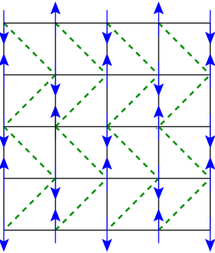
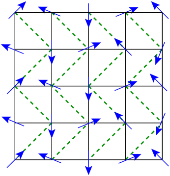
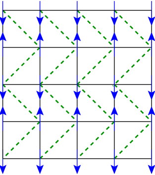
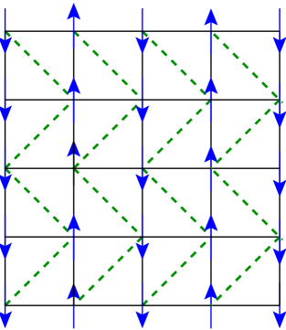
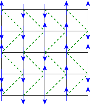
Figure 1: (Color online) The $J_{1}$–$J_{2}$ chevron-square lattice model ($J_{1}\equiv 1$). The solid (black) lines are $J_{1}$ bonds and the dashed (green) lines are $J_{2}$ bonds; (a) Néel state, (b) spiral state (or state s), (c) row-striped state (or state r), (d) columnar-striped state (or state c), and (e) doubled alternating striped state (or state d). The blue arrows represent the spins on the sites of the chevron lattice.

Hence the square plaquettes along each row have the diagonal $J_{2}$ bond oriented in the same direction, and with that direction alternating between neighboring rows. On the chevron lattice each site is thus six-connected, as in the APP and interpolating square-triangle HAF models.

In view of the fact that other depleted $J_{1}$–$J_{2}$ models on the square lattice show such a rich variety of GS phase diagrams, the chevron-square lattice model now seems to be well worth studying theoretically too for the case $s=\frac{1}{2}$. The recent experimental quantum simulation of frustrated magnetism in triangular optical lattices,Struck:2011 which exploited the motional degrees of freedom of ultracold atoms, provides a clear additional impetus for such studies. In the experimental simulationStruck:2011 a specific modulation of the optical lattice was used to tune the NN couplings on the triangular lattice in different directions independently. By introducing a fast oscillation of the lattice the experimentalists were thus able to simulate our previous interpolating square-triangle AFM model.Bi:2009_SqTriangle Since, as we discuss below in Sec. II, the $J_{1}$–$J_{2}$ chevron-square lattice model may also equivalently be regarded as a different form of anisotropic triangular-lattice HAF, it is conceivable that this model too may be experimentally realizable with ultracold atoms trapped on a 2D triangular optical lattice.

In Sec. II we describe the model itself further, including its classical ($s\rightarrow\infty$) counterpart. The key elements of the CCM technique that we will apply to the $s=\frac{1}{2}$ model are reviewed in Sec. III, before presenting our results in Sec. IV. We end with a brief summary in Sec. V.

II THE MODEL

In this paper we study the chevron-square lattice model whose Hamiltonian may be written as

$$H=J_{1}\sum_{\langle i,j\rangle}\mathbf{s}_{i}\cdot\mathbf{s}_{j}+J_{2}\sum_{\langle\langle i,k\rangle\rangle^{\prime}}\mathbf{s}_{i}\cdot\mathbf{s}_{k}$$ (1)

where the operators $\mathbf{s}_{l}\equiv(s^{x}_{l},s^{y}_{l},s^{z}_{l}$) are the quantum spin operators on lattice site $l$, with $s^{2}_{l}=s(s+1)$. We are interested here in the extreme quantum case $s=\frac{1}{2}$. On the square lattice the sum over $\langle i,j\rangle$ runs over all distinct NN bonds (with exchange coupling strength $J_{1}$), while the sum over $\langle\langle i,k\rangle\rangle^{\prime}$ runs over only half of the distinct NNN diagonal bonds (with exchange coupling strength $J_{2}$). In the latter sum only one NNN diagonal bond is retained in each square plaquette, as arranged in the (vertical) chevron pattern shown explicitly in Fig. 1. The primitive unit cell is thus of size $1\times 2$. In both sums in Eq. (1) each bond is counted once and once only. In the present paper we consider the case where both sorts of bonds are AFM in nature, $J_{1}>0$ and $J_{2}\equiv\kappa J_{1}>0$, and hence act to frustrate one another. Henceforth, we put $J_{1}\equiv 1$ to set the overall energy scale.

The model may clearly equivalently be defined on a triangular-lattice geometry in which every site has six NN sites, four connected to it by $J_{1}$ bonds and two connected to it by $J_{2}$ bonds, as shown explicitly in Fig. 2.

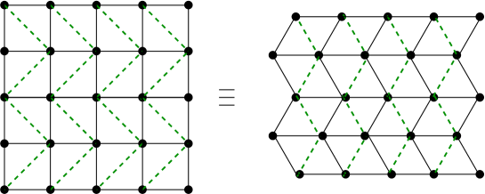
Figure 2: (Color online) The $J_{1}$–$J_{2}$ chevron-square lattice model as an equivalent anisotropic triangular-lattice HAF model.

Thus, the chevron-square lattice model may be regarded also as an anisotropic HAF on a triangular lattice, in which every basic triangular plaquette contains two NN $J_{1}$ bonds and one NN $J_{2}$ bond in the pattern shown. It thus clearly shares some properties with our previous interpolating square-triangle modelBi:2009_SqTriangle in the sense that both models interpolate smoothly between the HAF on the square lattice (when the NNN bonds retained on the square lattice are removed entirely) and the HAF on the triangular lattice (when both NN and the retained NNN bonds on the square lattice have equal strength). Both models can be regarded too as anisotropic triangular-lattice HAF models. Whereas our former interpolating square-triangle modelBi:2009_SqTriangle had the NN bonds along two of the three equivalent triangular-lattice directions equal ($J_{1}$) and different along the third direction ($J_{2}^{\prime}$), in the current chevron-lattice model the inequivalent ($J_{2}$) bonds are those along parallel zigzag (or chevron) chains in one of the three equivalent directions for the triangular lattice, as shown in Fig. 2.

The current model clearly also reduces to decoupled 1D chains in the limit $\kappa\rightarrow\infty$. Thus, the case $\kappa\gg 1$ corresponds to weakly coupled 1D chains, and the model thus also interpolates between 1D and 2D limits.

Before considering the extreme quantum limit $s=\frac{1}{2}$ it is worthwhile to examine first the classical limit, $s\rightarrow\infty$. Thus, it is easy to show that the classical chevron-square lattice model has only two GS phases. For $\kappa<\frac{1}{2}$ the stable GS phase has AFM Néel ordering on the square lattice, as shown in Fig. 1(a). At $\kappa=\kappa_{{\rm cl}}=\frac{1}{2}$ the system undergoes a continuous second-order phase transition to a state with noncollinear spiral order that persists for all values $\kappa>\frac{1}{2}$. The spin direction in this spiral state, shown in Fig. 1(b), at lattice site ($i,j$) points at an angle $\alpha_{ij}=\alpha_{0}+[i+\Delta(j)]\alpha$, where $\Delta(j)$ is defined to be zero if $j$ is even and one if $j$ is odd. The GS energy per spin in this classical spiral state is thus given by

$$\frac{E}{N}=s^{2}(2\cos\alpha+\kappa\cos 2\alpha)\,,$$ (2)

which is minimized when

$$\alpha=\alpha_{{\rm cl}}=\left\{\begin{array}[]{rl}\pi\,;&\quad\kappa\leq\frac{1}{2}\\ \cos^{-1}(-\frac{1}{2\kappa})\,;&\quad\kappa>\frac{1}{2}\,.\end{array}\right.$$ (3)

The pitch angle $\phi\equiv\pi-\alpha$ thus measures the deviation from Néel order, and its classical value is

$$\phi_{{\rm cl}}=\left\{\begin{array}[]{rl}0\,;&\quad\kappa\leq\frac{1}{2}\\ \cos^{-1}(\frac{1}{2\kappa})\,;&\quad\kappa>\frac{1}{2}\,.\end{array}\right.$$ (4)

It varies from zero for $\kappa<\kappa_{{\rm cl}}=\frac{1}{2}$ to $\frac{1}{2}\pi$ as $\kappa\rightarrow\infty$ (as shown later in Fig. 4). At the isotropic point, $\kappa=1$, we regain the classical three-sublattice ordering of the isotopic triangular-lattice HAF with $\alpha_{{\rm cl}}=\frac{2}{3}\pi$.

The GS energy per spin of the classical model is thus given by

$$\frac{E}{Ns^{2}}=\left\{\begin{array}[]{rl}-2+\kappa\,;&\quad\kappa\leq\frac{1}{2}\\ -(\frac{1}{2\kappa})-\kappa\,;&\quad\kappa>\frac{1}{2}\,.\end{array}\right.$$ (5)

Equation (5) clearly shows that the classical phase transition at $\kappa=\frac{1}{2}$ is a continuous (second-order) one, where both the GS energy and its first derivative with respect to the frustration parameter $\kappa$ are continuous.

In the limit of large $\kappa$ the GS configuration of the classical chevron-square lattice model represents a set of decoupled 1D HAF chains (along the chevrons of the model) with sites connected by $J_{2}$ bonds, and with a relative spin orientation approaching $90^{\circ}$ between sites on neighbouring chevrons. In this classical $\kappa\rightarrow\infty$ limit there is, however, also complete degeneracy between all states for which the relative ordering directions of spins on different HAF chevron chains is arbitrary. Clearly the spin-1/2 model also similarly reduces in the $\kappa\rightarrow\infty$ limit to a set of decoupled 1D HAF chevron chains, which exhibit the 1D Luttinger-liquid behavior described by the exact Bethe ansatz solution.Bethe:1931

In general quantum fluctuations tend to favor states with collinear spin order over ones with noncollinear order, and it thus seems possible that at sufficiently large (but finite) values of $\kappa$ the classical spiral order will be destroyed by quantum fluctuations in the spin-1/2 model of interest here, to yield a state with collinear spin ordering. In this case the probable ordering is thus clearly one with all of the 1D chevron chains exhibiting Néel ordering in the same direction, with spins alternating in orientation (say, up and down). We note that there is still an infinite family of such states in which, for example, all of the spins along a given row (in our convention) can be assigned arbitrarily to be either up or down. All of these states are degenerate in energy at the classical level, with an energy per spin given $E/N=-s^{2}\kappa$. They include, for example, the three states shown in Figs. 1(c), 1(d), and 1(e) in which, respectively, the spins in a given row all have the same orientation (e.g., $\uparrow\uparrow\uparrow\uparrow\uparrow\cdots$), alternate in orientation (e.g., $\downarrow\uparrow\downarrow\uparrow\downarrow\cdots$), and alternate in orientation in a pairwise fashion (e.g., $\downarrow\downarrow\uparrow\uparrow\downarrow\cdots$). Henceforth, we refer to these three states respectively as the row-striped state (or state r), the columnar-striped state (or state c), and the doubled alternating striped state (or state d).

Clearly, from Eq. (5), the classical spiral state (or state s) always has lower energy than this classical infinitely-degenerate family of collinear AFM states. Hence, unlike in the classical APP model, where the corresponding infinitely-degenerate family of crossed 1D HAF chains does form the stable GS phase for all values $\kappa>1$, this family never becomes the stable GS phase for the classical chevron-lattice model except in the $\kappa\rightarrow\infty$ limit. Nevertheless, as we have already suggested, it does form a likely candidate for the stable GS phase of the $s=\frac{1}{2}$ version of the model considered below, as we discuss further in Sec. IV. In this case we also expect that the (accidental) classical degeneracy might again be lifted by the order by disorder mechanism.

III THE COUPLED CLUSTER METHOD

The CCMBishop_1987:ccm ; Arponen:1991_ccm ; Bi:1991 ; Bishop:1998 ; Fa:2004 that we use here has become one of the most powerful and most universally applicable techniques of modern microscopic quantum many-body theory. In recent times it has been applied with great success to a large variety of quantum spin-lattice systems (see, e.g., Refs. Bishop:1991_ccm, ; Ze:1998, ; Kr:2000, ; Bishop:2000, ; Fa:2001, ; schmalfuss, ; Fa:2004, ; Darradi:2005, ; Darradi:2008_J1J2mod, ; Bi:2008_JPCM, ; Bi:2008_PRB_J1xxz_J2xxz, ; Bi:2009_SqTriangle, ; richter10, ; UJack_ccm, ; Reuther:2011_J1J2J3mod, ; Farnell:2011, ; Gotze:2011, ; Bishop:2012_checkerboard, ; Li:2012_honey_full, ; Li:2012_anisotropic_kagomeSq, and references cited therein). In particular, for 2D models of quantum magnetism, it now provides one of the most accurate methods available for their study. Some of its most notable strengths are that it provides a systematic way to study various candidate GS phases and their regions of stability, and that in each case the description is systematically improvable in terms of well-defined hierarchies of approximations to incorporate more and more of the multispin configurations present in the exact, fully correlated, GS wave function.

The CCM formalism is now briefly presented. We concentrate on its key ingredients only, as needed for present purposes, and refer the interested reader to the extensive literature on the method (see, e.g., Refs. Bishop_1987:ccm, ; Arponen:1991_ccm, ; Bi:1991, ; Bishop:1998, ; Fa:2004, ; Ze:1998, ; Kr:2000, ; Bishop:2000, ) for further details. Any implementation of the CCM always begins with the selection of some suitable (normalized) model (or reference) state $|\Phi\rangle$. For spin-lattice models this is often conveniently chosen as a classical state, which may or may not form the actual GS phase of the classical ($s\rightarrow\infty$) version of the model in some region of the $T=0$ parameter space. For the present chevron-square lattice model we will present below in Sec. IV results based on all five of the states shown in Fig. 1 as CCM model states, for reasons already outlined in Sec. II.

We denote by $|\Psi\rangle$ and $\langle\tilde{\Psi}|$ respectively the exact GS ket and bra wave functions of the fully interacting system under study, where the normalizations are chosen so that $\langle\tilde{\Psi}|\Psi\rangle=\langle\Phi|\Psi\rangle=\langle\Phi|\Phi\rangle=1$. The CCM now uses the exponential parametrizations

$$|\Psi\rangle={\rm e}^{S}|\Phi\rangle\,;\quad\langle\tilde{\Psi}|=\langle\Phi|\tilde{S}{\rm e}^{-S}\,,$$ (6)

to incorporate explicitly the multispin-flip configurations in $|\Psi\rangle$ and $\langle\tilde{\Psi}|$ above and beyond those contained in the chosen model state $|\Phi\rangle$. The ket- and bra-state correlation operators are then expressed as

$$S=\sum_{I\neq 0}{\cal S}_{I}C^{+}_{I}\,;\quad\tilde{S}=1+\sum_{I\neq 0}{\cal\tilde{{S}}}_{I}C^{-}_{I}\,,$$ (7)

where, by definition, $C^{+}_{0}\equiv 1$ is the identity operator, and $C^{-}_{I}|\Phi\rangle=0=\langle\Phi|C^{+}_{I},\forall I\neq 0$. The set-index $\{I\}$ represents a multispin-flip configuration with respect to state $|\Phi\rangle$, as we elaborate further below. The operator $C^{+}_{I}$ ($\equiv(C^{-}_{I})^{\dagger}$) thus represents a multispin-flip creation operator with respect to $|\Phi\rangle$ considered as a generalized vacuum state.

It is now convenient to choose a set of local coordinate frames in spin space defined for each model state separately, such that on each lattice site the spin aligns along the negative $z$ axis (downwards). Such rotations obviously leave the basic SU(2) spin commutation relations unchanged. In such a basis the $C^{+}_{I}$ operators now have the universal form, $C^{+}_{I}\equiv s^{+}_{j_{1}}s^{+}_{j_{2}}\cdots s^{+}_{j_{n}}$ in terms of the usual single-spin raising operators $s^{+}_{j}\equiv s^{x}_{j}+is^{y}_{j}$. For a spin $s$ the raising operator $s^{+}_{j}$ may be applied a maximum of 2$s$ times on a given site $j$, and hence the set-index $\{I\}\equiv\{j_{1},j_{2},\cdots,j_{n};\,n=1,2,\cdots\}$ where any given site-index $j_{k}$ may appear a maximum of 2$s$ times. In the present $s=\frac{1}{2}$ case therefore, no index may be repeated.

The ket- and bra-state coefficients $\{{\cal S}_{I},\tilde{\cal S}_{I}\}$, which from Eqs. (6) and (7) completely specify the GS wave function, may now be obtained by minimizing the GS energy functional, $\bar{H}=\bar{H}({\cal S}_{I},\tilde{\cal S}_{I})\equiv\langle\tilde{\Psi}|H|\Psi\rangle$, where $H$ is the Hamiltonian of the system, with respect to all of the coefficients $\{\tilde{\cal S}_{I}\}$ and $\{{\cal S}_{I}\}$ separately, $\forall I\neq 0$. Use of Eqs. (6) and (7) then leads simply to the respective coupled sets of equations $\langle\Phi|C^{-}_{I}{\rm e}^{-S}H{\rm e}^{S}|\Phi\rangle=0$ and $\langle\Phi|\tilde{{\cal S}}{\rm e}^{-S}[H,C^{+}_{I}]{\rm e}^{S}|\Phi\rangle=0;\forall I\neq 0$, which are fully equivalent to the GS ket and bra Schrödinger equations $H|\Psi\rangle=E|\Psi\rangle$ and $\langle\tilde{\Psi}|H=E\langle\tilde{\Psi}|$. The latter set of equations may equivalently be written as $\langle\Phi|\tilde{S}({\rm e}^{-S}H{\rm e}^{S}-E)C^{+}_{I}|\Phi\rangle=0,\forall I\neq 0$.

Once these sets of CCM equations have been solved for the sets of correlation coefficients $\{{\cal S}_{I}\}$ and $\{\tilde{\cal S}_{I}\}$, all GS quantities may now be calculated in terms of them. The GS energy is unique in that its evaluation requires only the ket-state coefficients, $E=\langle\Phi|{\rm e}^{-S}H{\rm e}^{S}|\Phi\rangle$, whereas any other GS quantity requires the bra-state coefficients also. For present purposes, for example, we will also calculate the magnetic order parameter, defined to be the local average on-site magnetization, $M$, in the rotated spin coordinates, $M\equiv-\frac{1}{N}\langle\tilde{\Psi}|\sum^{N}_{j=1}s^{z}_{j}|\Psi\rangle$, where $N$ is the number of lattice sites. A key feature of the CCM exponential parametrizations of Eq. (6) is that the method automatically satisfies the Goldstone linked cluster theorem, even when truncations are made in the multispin configurations $\{I\}$ retained in Eq. (7). Thus, the method is automatically size-extensive at every level of approximation, and we may take the infinite-lattice limit, $N\rightarrow\infty$, from the very outset. Similarly, the method also satisfies the Hellmann-Feynman theorem at all levels of truncation.

It is important to note too that while the CCM equations are intrinsically nonlinear, due to the presence of the basic correlation operator $S$ in the exponentiated form ${\rm e}^{S}$, it only ever appears in the equations to be solved in the similarity transform, ${\rm e}^{-S}H{\rm e}^{S}$, of the Hamiltonian. By making use of the well-known nested commutator expansion for ${\rm e}^{-S}H{\rm e}^{S}$, it is readily seen that the basic SU(2) spin commutation relations imply that the otherwise infinite series of nested commutators actually terminates exactly at second-order terms in $S$ for Hamiltonians of the form of Eq. (1) used here (and see, e.g., Refs. Fa:2004, ; Ze:1998, for further details). A similar exact termination generally also applies to the evaluation of the GS expectation value of any operator, such as $M$ above, that we calculate.

Thus, the CCM formalism is exact if all multispin-flip configurations are included in the index-set $\{I\}$, and the equations that we need to solve in practice are coupled sets of multinomial equations for the coefficients $\{{\cal S}_{I}\}$ and linear equations for the coefficients $\{\tilde{\cal S}_{I}\}$, in which the solutions for $\{{\cal S}_{I}\}$ are needed as input. Of course, in practice we need to make finite-size truncations in the multispin-flip configurations retained in the indices $\{I\}$. We employ here the localized (lattice-animal-based subsystem) LSUB$n$ scheme,Fa:2004 ; Ze:1998 which has been well-studied and greatly utilized for a wide variety of spin-1/2 lattice systems.Bishop:1991_ccm ; Ze:1998 ; Kr:2000 ; Bishop:2000 ; Fa:2001 ; schmalfuss ; Fa:2004 ; Darradi:2005 ; Darradi:2008_J1J2mod ; Bi:2008_JPCM ; Bi:2008_PRB_J1xxz_J2xxz ; Bi:2009_SqTriangle ; richter10 ; UJack_ccm ; Reuther:2011_J1J2J3mod ; Farnell:2011 ; Gotze:2011 ; Bishop:2012_checkerboard ; Li:2012_honey_full ; Li:2012_anisotropic_kagomeSq At the nth level of approximation in the LSUB$n$ scheme all possible multispin-flip configurations are retained in the index-set $\{I\}$ over different locales on the lattice defined by $n$ or fewer contiguous sites. In other words, all lattice animals of size up to $n$ sites are populated with flipped spins (with respect to the model state $|\Phi\rangle$ as reference state) in all possible ways. Such animals (or contiguous clusters) are defined to be contiguous in this sense if every site in the cluster is adjacent (in the NN sense) to at least one other site in the cluster. For our present model we define NN pairs on the triangular-lattice geometry (as shown in Fig. 2), rather than on the square-lattice geometry, since we wish to treat all pairs connected by both $J_{1}$ and $J_{2}$ bonds on an equal footing.

The number $N_{f}$ of such fundamental configurations, which are distinct under the space- and point-group symmetries of the lattice and of the model state being used, increases very rapidly with the truncation index $n$ of the LSUB$n$ hierarchy. In the present study, by making use of a highly efficient parallelized CCM codecccm and supercomputer resources we have been able to perform LSUB$n$ calculations up to the LSUB10 level for each of the four collinear model states of Figs. 1(a), (c), (d), and (e), and up to the LSUB8 level for the spiral state of Fig. 1(b). For example, using the triangular-lattice geometry, $N_{f}=541578$ for the LSUB10 approximation using the row-striped state of Fig. 1(c) as CCM model state.

Although we never need to perform any finite-size scaling of our results, since we work from the outset in the thermodynamic limit, $N\rightarrow\infty$, we do need to extrapolate our approximate LSUB$n$ sequence for any physical quantity to the exact $n\rightarrow\infty$ limit. For example, for the GS energy per spin, $E/N$, we use the well-tested extrapolation scheme Kr:2000 ; Bishop:2000 ; Fa:2001 ; Darradi:2005 ; schmalfuss ; Bi:2008_PRB_J1xxz_J2xxz ; Darradi:2008_J1J2mod ; Bi:2008_JPCM ; richter10 ; Reuther:2011_J1J2J3mod ; Bishop:2012_checkerboard ; Li:2012_anisotropic_kagomeSq

$$E(n)/N=a_{0}+a_{1}n^{-2}+a_{2}n^{-4}\,.$$ (8)

As is to be expected other physical quantities do not converge as rapidly as the energy. For example, for the magnetic order parameter, $M$, we generally find that a scaling law with leading power $1/n$, i.e.,

$$M(n)=b_{0}+b_{1}n^{-1}+b_{2}n^{-2}\,,$$ (9)

works well for most systems with even moderate amounts of frustration. Kr:2000 ; Bishop:2000 ; Fa:2001 ; Darradi:2005 However, for systems very close to a QCP or for which the magnetic order parameter of the phase under study is very small or zero, the scaling law of Eq. (9) has been found to overestimate the magnetic order and to predict a too large value for the critical value of the the frustration parameter that is driving the transition. In such cases we use the well-studied extrapolation schemeDarradi:2005 ; schmalfuss ; Bi:2008_JPCM ; Bi:2008_PRB_J1xxz_J2xxz ; Darradi:2008_J1J2mod ; richter10 ; Reuther:2011_J1J2J3mod ; Bishop:2012_checkerboard ; Li:2012_anisotropic_kagomeSq

$$M(n)=c_{0}+c_{1}n^{-1/2}+c_{2}n^{-3/2}\,.$$ (10)

Naturally, for any physical quantity $Q$ we may always test for the correct leading power in the corresponding LSUB$n$ extrapolation scheme by first fitting to a form

$$Q(n)=q_{0}+q_{1}n^{-\nu}\,,$$ (11)

where the exponent $\nu$ is also a fitting parameter. For the GS energy we generally find a value $\nu\approx 2$ for a wide variety of both unfrustrated and (strongly) frustrated systems, as is also the case here, as we discuss in Sec. IV in more detail. On the other hand, for the magnetic order parameter, $M$ we find $\nu\approx 1$ for many systems, even moderately frustrated systems such as the triangular-lattice HAF, which is the special case $\kappa=1$ of the present model. However, in situations where we are either close to a transition or where $M$ is (close to) zero for the phase under study we generally find $\nu\approx 0.5$. Both cases are present in the current model, as we discuss more fully in Sec. IV. Once such values for the leading exponent have been found, they provide the subsequent rationale for the use of Eqs. (8)–(10), for example.

IV RESULTS

We report here on our CCM calculations for the present spin-1/2 $J_{1}$–$J_{2}$ chevron-square lattice model of Eq. (1) based in turn on each of the Néel, spiral, row-striped, columnar-striped, and doubled alternating striped states shown, respectively in Figs. 1(a,b,c,d,e). The computational power at our disposal is such that we can perform LSUB$n$ calculations for each of the collinear model states with $n\leq 10$, but for the more exacting spiral model state only for $n\leq 8$.

In the first place we discuss our results obtained using the spiral model state. Whereas the classical ($s\rightarrow\infty$) version of the model has a second-order phase transition from Néel order (for $\kappa<\kappa_{{\rm cl}}$) to spiral order (for $\kappa>\kappa_{{\rm cl}}$) at the value $\kappa=\kappa_{{\rm cl}}=0.5$ of the frustration parameter, our CCM results show a shift of this critical point to a value $\kappa=\kappa_{{\rm cl}}\approx 0.72$ for the present $s=\frac{1}{2}$ quantum case. This finding is in complete agreement with the general observation, which is found to be true for a wide variety of different spin-lattice models, that quantum fluctuations generally favor collinear over noncollinear forms of spin ordering, as discussed previously in Sec. II.

Curves such as those shown in Fig. 3 show clearly that the CCM results based on the Néel model state (with $\phi=0$) give the minimum GS energy for all values of $\kappa<\kappa_{c_{1}}$, where our estimate for $\kappa_{c_{1}}$ is itself dependent on the level of LSUB$n$ approximation used, as may be seen from Fig. 4.

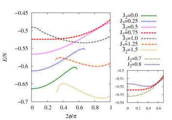
Figure 3: (Color online) Ground-state energy per spin, $E/N$, as a function of the spiral angle $\phi$, of the spin-1/2 $J_{1}$–$J_{2}$ chevron-square lattice model ($J_{1}\equiv 1$, $J_{2}>0$). We show results using the LSUB4 approximation of the CCM based on the spiral model state for some illustrative values of $J_{2}$ in the range $0\leq J_{2}\leq 1.5$. For $J_{2}\lesssim 0.752$ the minimum is at $\phi=0$ (Néel order), whereas for $J_{2}\gtrsim 0.752$ the minimum occurs at $\phi=\phi_{{\rm LSUB}4}\neq 0$, signalling a phase transition at $J_{2}\approx 0.752$ in this approximation.

The general shape of the curves shown in Fig. 3 is broadly similar to that of their classical counterparts, $E/N=s^{2}(\kappa\cos 2\phi-2\cos\phi$), from Eq. (2), but with several important differences. One is that the crossover from the minimum being at $\phi=0$ (Néel order) to a value $\phi>0$ (spiral order) occurs at an appreciably higher value $\kappa_{c_{1}}\approx 0.72$ in the $s=\frac{1}{2}$ case than at the value $\kappa_{{\rm cl}}=0.5$ for the classical ($s\rightarrow\infty$) case. Another difference is that the crossover curve itself becomes even flatter in the spin-1/2 case than in the classical case.

Thus, a close inspection of curves such as those displayed in Fig. 3 for the LSUB4 case shows that, at this level of approximation, for example, for all values $\kappa\lesssim 0.752$ the only minimum in the GS energy is at $\phi=0$. When this value is approached asymptotically from below the LSUB4 energy curves become very flat around $\phi=0$, indicating the disappearance at $\phi=0$ not only of the second derivative ${\rm d}^{2}E/{\rm d}\phi^{2}$ but probably also of one or more of the higher derivatives ${\rm d}^{n}E/{\rm d}\phi^{n}$ with $n>2$ (as well as the first derivative ${\rm d}E/{\rm d}\phi$). Similar curves occur for other LSUB$n$ approximations. By contrast, in the classical case, at $\kappa=\kappa_{{\rm cl}}$, ${\rm d}^{n}E/{\rm d}\phi^{n}$ vanishes only for $n\leq 2$. For values $\kappa>\kappa_{{\rm cl}}$ the classical curves now have a maximum at $\phi=0$ and a minimum at the value $\phi_{{\rm cl}}$ given by Eq. (4). This behavior is broadly echoed in the LSUB4 $s=\frac{1}{2}$ curves shown in Fig. 3 for $\kappa>\kappa_{c_{1}}$.

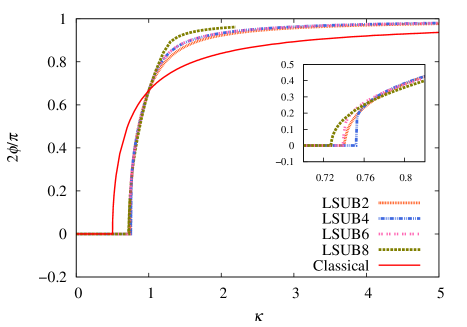
Figure 4: The angle $\phi_{{\rm LSUB}n}$ that minimizes the energy per spin, $E_{{\rm LSUB}n}(\phi)/N$, of the spin-1/2 $J_{1}$–$J_{2}$ chevron-square lattice model (with $J_{1}>0$) versus the frustration parameter $\kappa\equiv J_{2}/J_{1}$, in the LSUB$n$ approximations with $n=\{2,4,6,8\}$ based on the spiral model state. The corresponding classical result, $\phi_{{\rm cl}}$, of Eq. (4) is also shown for comparison.

However, we note from Fig. 4 (and see especially the inset) that the crossover from one minimum ($\phi=0$, Néel) solution to the other ($\phi\neq 0$, spiral) one appears to be rather abrupt, particularly for the LSUB$n$ approximations with $n=4,6$, with the pitch angle rising very sharply from a zero value on the Néel side to a nonzero value on the spiral side. This very sharp rise is itself just a reflection of the extreme flatness of the corresponding GS energy curves in Fig. 3 near the crossover point $\kappa=\kappa_{{\rm cl}}$. This very flatness makes it difficult for us to distinguish between the two scenarios of a discontinuous jump in pitch angle versus a continuous but very steep rise in pitch angle as we traverse the transition in the frustration parameter $\kappa$ from the Néel phase into the spiral one. These two scenarios would correspond, respectively, to a weakly first-order transition versus a (continuous) second-order one. More compelling evidence for both the numerical value $\kappa_{c_{1}}$ and the nature of the Néel-spiral quantum phase transition comes from our results, presented below, for the local on-site magnetization (which provides the relevant order parameter for the transition).

However, before doing so, we comment further on Figs. 3 and 4. Firstly, we see from Fig. 3 that all of the CCM LSUB$n$ approximation give exactly the classical value $\phi=\frac{1}{3}\pi$ for the pitch angle at the value $\kappa=1$ corresponding to the spin-1/2 HAF on the triangular lattice. This corresponds to the correct $120^{\circ}$ three-sublattice ordering demanded by symmetry in this case. The fact that every LSUB$n$ approximation preserves this symmetry is a simple consequence of us defining the fundamental LSUB$n$ configurations on the triangular-lattice geometry shown in Fig. 2 (in which sites connected by both $J_{1}$ and $J_{2}$ bonds are defined to be NN pairs). By contrast, had we defined the fundamental LSUB$n$ configurations on the underlying square-lattice geometry (in which only sites connected by $J_{1}$ bonds are NN pairs, and where sites connected by $J_{2}$ bonds are NNN pairs), the exact symmetry at $\kappa=1$ would only be approximately preserved in any LSUB$n$ approximation with a finite value of $n$.

We also note from Fig. 4 that when $\kappa>1$ the pitch angle $\phi$ approaches the asymptotic ($\kappa\rightarrow\infty$) limiting value $\frac{1}{2}\pi$ much faster for the quantum $s=\frac{1}{2}$ model than for its classical ($s\rightarrow\infty$) counterpart. This is a first direct piece of evidence that quantum fluctuations favor, in this limit, collinear ordering along the weakly coupled 1D chevron chains. Figure 4 also shows that the CCM LSUB8 approximation based on the spiral model state appears slightly anomalous in the region $\kappa>1$, with the solution even becoming unstable for values $\kappa\gtrsim 2.2$. We take this as a first indication that the quantum spiral state itself loses its stability as the actual GS phase in this regime, as we discuss much more fully below.

Before doing so, however, we note first from Fig. 3 that our CCM solutions at a given LSUB$n$ level of implementation (viz., LSUB4 in Fig. 3) exist only for certain ranges of the spiral pitch angle $\phi$ for some values of $\kappa$. Thus, for example, for the case $\kappa=0$ pertaining to the pure square-lattice HAF (with NN interactions only), the CCM LSUB4 solution based on the spiral model state of Fig. 1(b) only exists for values of the frustration parameter in the range $0\leq\kappa\lesssim 0.29\pi$. For this value $\kappa=0$, where the Néel state is the physical GS phase, it seems that any attempt to drive the system too far away from collinearity leads to the CCM solutions themselves becoming unstable in the sense that a real solution simply ceases to exist. Similarly, for example, when $\kappa=1.5$, Fig. 3 shows that the CCM LSUB4 solution exists only for values $0.15\pi\lesssim\kappa\lesssim 0.5\pi$. In this case the spiral state provides the stable GS phase, and any attempt now to move too close to collinearity leads again to instability.

Similar instabilities, which manifest themselves as termination points, occur in all LSUB$n$ approximation (with $n>2$). Indeed, such terminations of CCM solutions are both very common and well understood (see, e.g., Refs. Fa:2004, ; Bi:2009_SqTriangle, ). They are always reflections of the actual quantum phase transitions in the system under study. In the present case this is simply the transition between the Néel and spiral phases.

In view of the fact that we have indications or suggestions that the classical spiral phase might become unstable (for larger values of the frustration parameter $\kappa$) against quantum fluctuations, we have also performed CCM calculations based on the three other collinear states shown in Fig. 1(c), 1(d), and 1(e). All of these share the feature that the magnetic ordering along each chevron chain (i.e., sites joined by $J_{2}$ bonds) is that of a 1D Néel HAF. As explained in Sec. II, there is actually an infinite family of such states, all of which are degenerate in energy at the classical level. As expected, Fig. 5 now shows that this accidental classical degeneracy is lifted by quantum fluctuations.

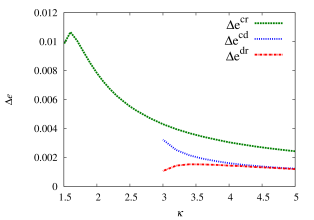
Figure 5: (Color online) Various GS energy differences, $\Delta e^{\rm ab}\equiv e^{{\rm state\;a}}-e^{{\rm state\;b}}$, with $e\equiv E/N$, between states a and b, versus the frustration parameter $\kappa\equiv J_{2}/J_{1}$, for the spin-1/2 chevron-square lattice model (with $J_{1}>0$), where states a and b are chosen to be the states r (row-striped), c (columnar-striped), and d (doubled alternating striped) of Figs. 1(c)–(e), respectively. In each case the energy per spin, $e$, is the LSUB$\infty$ result obtained from Eq. (8) using CCM LSUB$n$ results with $n=\{4,6,8,10\}$.

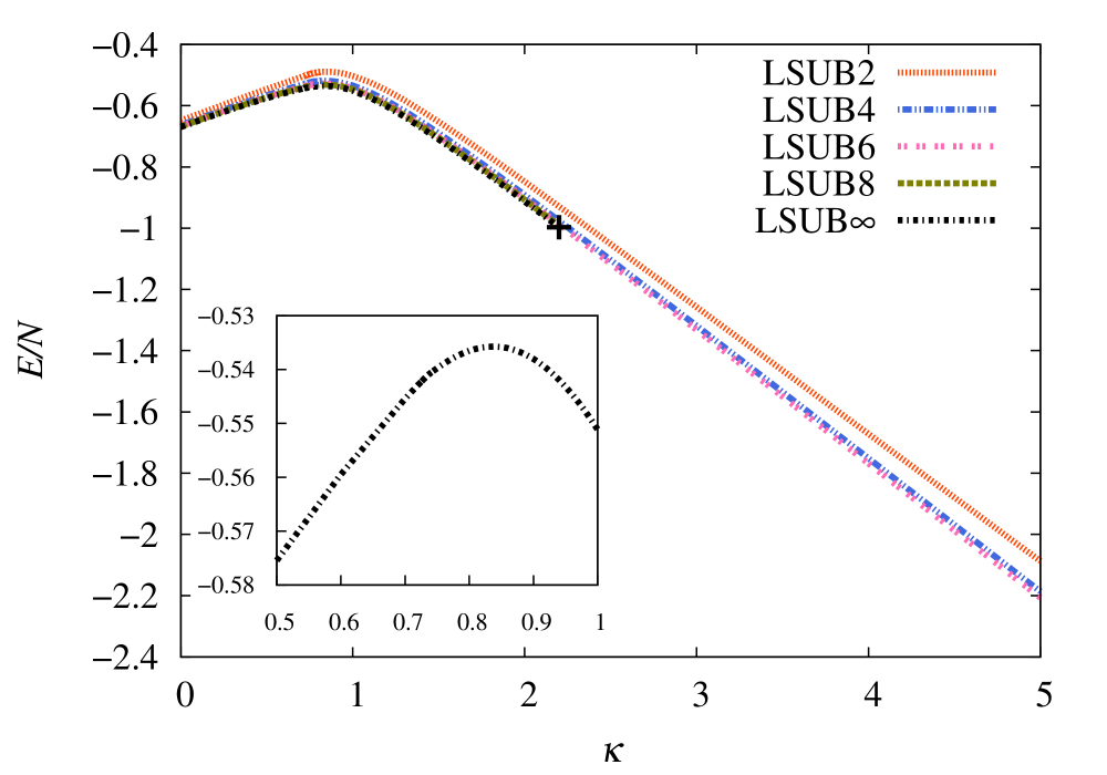
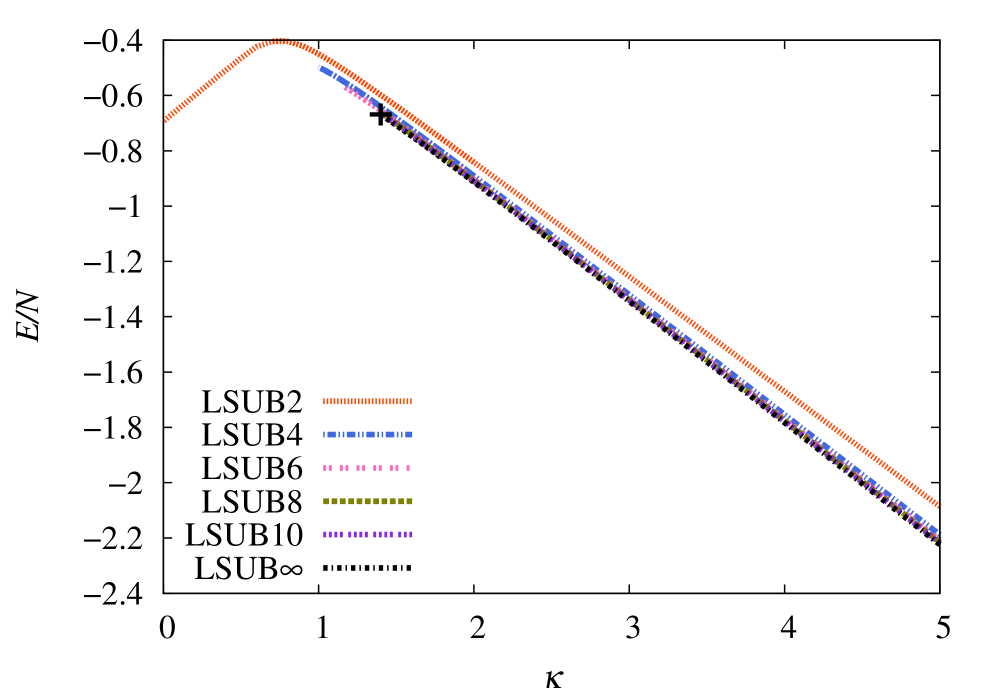
Figure 6: (Color online) CCM LSUB$n$ results for the GS energy per spin, $E/N$, versus the frustration parameter $\kappa\equiv J_{2}/J_{1}$, for the spin-1/2 $J_{1}$–$J_{2}$ chevron-square lattice model (with $J_{1}>0$), using (a) the Néel and spiral states of Figs. 1(a) and 1(b) respectively as model states with $n=\{2,4,6,8\}$, and (b) the row-striped state of Fig. 1(c) as model state, with $n=\{2,4,6,8,10\}$. In each case we also show the extrapolated LSUB$\infty$ result obtained from Eq. (8) using the data set $n=\{2,4,6,8\}$.

As a parenthetic note we add that in Fig. 5 the results using state d as CCM model state are shown only in the range $\kappa\geq 3$, since real solutions for all of the corresponding LSUB$n$ approximations used (viz., $n=\{4,6,8,10\}$) exist only in this range for this state. Corresponding terminations for states c and r occur only for values $\kappa<1.5$, as we discuss more fully below for state r. Although the differences in the energies between the three states are small, it is clear that the row-striped state of Fig. 1(c) has the lowest GS energy for all values of the frustration parameter, $\kappa$, shown. Henceforth, therefore, we only present results comparing CCM solutions based on the Néel, spiral, and row-striped states as model states.

Thus, firstly, in Fig. 6 we show our CCM results for the GS energy per spin, $e\equiv E/N$, based on each of these states as model states. We show both raw LSUB$n$ results and the corresponding extrapolated LSUB$\infty$ results using the extrapolation formula of Eq. (8). It is clear that the LSUB$n$ results based on each model state converge extremely rapidly as $n\rightarrow\infty$. Figure 6(a) shows that there is no real evidence for a discontinuity in slope at the critical values $\kappa_{c_{1}}$ (which themselves depend only weakly upon the order $n$ of the LSUB$n$ approximation used). If present at all, either in the raw LSUB$n$ results or the LSUB$\infty$ extrapolation, any such discontinuity can only be very weak indeed.

The overall accuracy of our results may also be ascertained by examining the special case of $\kappa=0$ (corresponding to the Néel order of the square-lattice HAF) and $\kappa=1$ (corresponding to the spiral, $\phi=\frac{1}{3}\pi$, order of the triangular-lattice HAF). Thus, for $\kappa=0$, the extrapolated GS energy per spin, using our LSUB$n$ results with $n=\{4,6,8,10\}$ is $e(\kappa=0)\approx-0.6697$, which may be compared with the results $e(\kappa=0)=-0.6693(1)$ from a linked-cluster series expansion (SE) technique,Zh:1991 and $e(\kappa=0)=-0.669437(5)$ from a large-scale quantum Monte Carlo (QMC) simulation,Sa:1997 free of the usual “minus-sign-problems” for this unfrustrated limiting case where the Marshall-Peierls sign rulesMa:1955 applies. Similarly, for $\kappa=1$, the extrapolated value using our LSUB$n$ results with $n=\{2,4,6,8\}$ is $e(\kappa=1)\approx-0.5511$, which may again be compared with the results $e(\kappa=1)=-0.5502(4)$ from a SE calculation,Zheng:2006 and $e(\kappa=1)=-0.5458(1)$ from a QMC simulation.Ca:1999 It is worth noting that, unlike for the square-lattice HAF, the nodal structure of the exact GS wave function for the triangular-lattice HAF is unknown. Hence, in this latter $\kappa=1$ case the QMC minus-sign problem cannot be avoided. Instead, a fixed-node approximation was made in Ref. Ca:1999, , which was then relaxed using a stochastic reconfiguration technique. The resulting approximate result for the GS is now only an upper bound, and our own CCM result is almost certainly more accurate in this case.

In both Figs. 6(a) and 6(b) the extrapolated results are shown only for those values of $\kappa$ in each case for which real solutions exist for all of the LSUB$n$ approximations used in the extrapolation. In the case of the spiral state used as CCM model states, shown in Fig. 6(a), the extrapolation is thus shown for the range $0<\kappa\lesssim 2.2$, since the LSUB8 solution shows an instability for $\kappa\gtrsim 2.2$ as discussed previously. Similarly, in Fig. 6(b), we can see that each of the LSUB$n$ results with $n>2$ based on the row-striped state as model state, terminate at some lower value, $\kappa_{t}(n)$, which itself depends on the level $n$ of approximation. Thus, we find $\kappa_{t}(4)\approx 0.95\pm 0.05$, $\kappa_{t}(6)\approx 1.15\pm 0.05$, $\kappa_{t}(8)\approx 1.35\pm 0.05$, and $\kappa_{t}(10)\approx 1.35\pm 0.05$.

As we have noted above, such termination points of our CCM LSUB$n$ calculations are always reflections of the true quantum phase transitions in the system.Fa:2004 ; Bi:2009_SqTriangle ; UJack_ccm They arise due to the solution to the CCM LSUB$n$ equations becoming complex there, such that beyond any such termination point two unphysical branches of complex conjugate solutions exist. Conversely, in the region where the true physical solution is real, there actually exists another (unstable) real solution, which is both unphysical and generally very difficult to determine numerically. The physical branch is also usually easily identifiable in practice as the one which becomes exact in some limiting case. At a termination point the two real branches of solution (physical and unphysical) meet, and then diverge again as wholly unphysical complex conjugate pairs beyond the termination point for real solutions. The values of $\kappa_{t}(n)$ may themselves be used to estimate the corresponding quantum critical point (QCP) $\kappa_{c}={\rm lim}_{n\rightarrow\infty}\kappa_{t}(n)$. We do not attempt to do so here since it is difficult to obtain values of $\kappa_{t}(n)$ with high precision, since the number of iterations required to solve the CCM LSUB$n$ equations to a given level of accuracy generally increases significantly as $\kappa\rightarrow\kappa_{t}(n)$. Furthermore, we have other more accurate criteria for determining the QCPs, as we discuss below. Nevertheless, even the crude values for $\kappa_{t}(n)$ above for $n=\{4,6,8,10\}$ indicate that the row-striped state itself can only be a possible candidate for the GS phase of our system for values of $\kappa\gtrsim 1.5$.

We show in Fig. 7 our CCM LSUB$\infty$ extrapolated results for the GS energy per spin, $e\equiv E/N$, based on the Néel, spiral and row-striped model states, using Eq. (8) and our corresponding LSUB$n$ results for the two data sets $n=\{2,4,6,8\}$ and $n=\{4,6,8,10\}$.

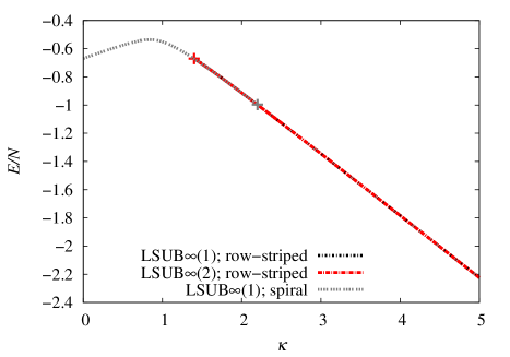
Figure 7: Extrapolated CCM LSUB$\infty$ results for the GS energy per spin, $E/N$, versus the frustration parameter $\kappa\equiv J_{2}/J_{1}$, for the spin-1/2 $J_{1}$–$J_{2}$ chevron-square lattice model (with $J_{1}>0$). We show results based on the Néel and spiral model states for $\kappa<2.2$, and on the row-striped model state for $\kappa>1.4$, where these two (LSUB8) termination points (see text) are marked by $+$ symbols. The LSUB$\infty$(1) and LSUB$\infty$(2) curves are extrapolations using Eq. (8) and LSUB$n$ results with $n=\{2,4,6,8\}$, and $n=\{4,6,8,10\}$ respectively.

We note in passing that if our LSUB$n$ results are instead fitted to a form $e(n)=e_{0}+e_{1}n^{-\nu}$, the fitted value for the exponent $\nu$ turns out to be very close to 2 for all values of $\kappa$ except those close to the termination points of the data set used, for each of our model states. The use of Eq. (8) is thereby again justified for this model. We see firstly from Fig. 7 that the results are almost identical using both data sets for the row-striped case illustrated. Similar insensitivity of our extrapolated results for the GS energy against the LSUB$n$ data set used holds for the other model states too. Secondly, we note how our extrapolated results based on both the spiral and row-striped states are very close to one another, although not identical, as we discuss further below. Thirdly, we note that in the $\kappa\rightarrow\infty$ (decoupled spin-1/2 1D HAF chevron chains) limit, the results shown in Fig. 7 for the row-striped state yield an extrapolated value of the energy per spin which approaches the value $E/N=-0.4431\kappa$, which agrees precisely with the exact result, $E/N=(\frac{1}{4}-\ln 2)\kappa$, from the Bethe ansatz solution.Bethe:1931 ; Hulthen:1938

In Fig. 8 we show directly the GS energy difference, $e\equiv E/N$, between the spiral and row-striped states.

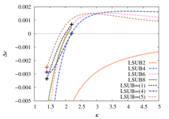
Figure 8: (Color online) The GS energy difference, $\Delta e^{{\rm sr}}\equiv e^{{\rm s}}-e^{{\rm r}}$, with $e\equiv E/N$, between the spiral (s) and row-striped (r) states versus the frustration parameter $\kappa\equiv J_{2}/J_{1}$, for the spin-1/2 chevron-square lattice model (with $J_{1}>0$). Results are shown using separate LSUB$n$ calculations for states s and r, with $n=\{2,4,6,8\}$, and also from separate LSUB$\infty(k)$ extrapolations for the states s and r using Eq. (8) and LSUB$n$ data sets separately: $k=1$, $n=\{2,4,6,8\}$; $k=4$, $n=\{4,6,8\}$; and $k=5$, $n=\{2,4,6\}$. The respective termination points for the states are shown by $+$ symbols.

We display both raw results at various LSUB$n$ levels of approximation and extrapolated results where we use Eq. (8) with various LSUB$n$ data sets for each state separately before taking the difference. In each case the extrapolated results are shown for values between the respective termination points for each of the two states. Although the energy difference is small, it is well within our level of accuracy.

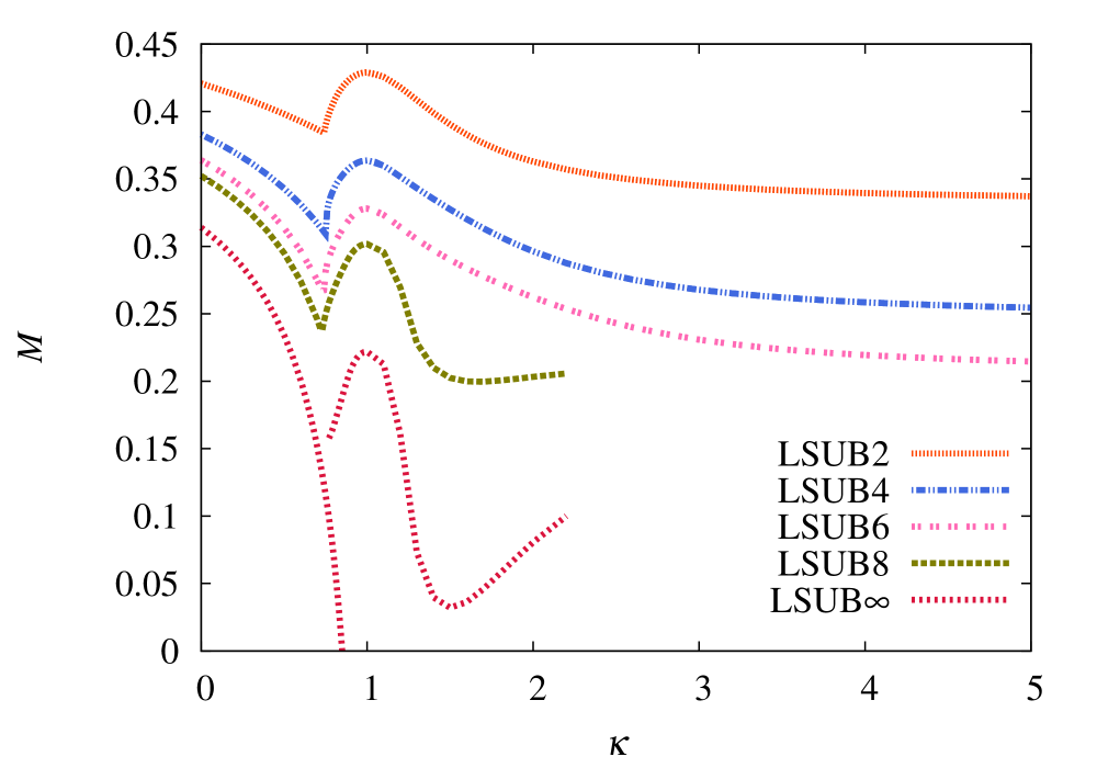
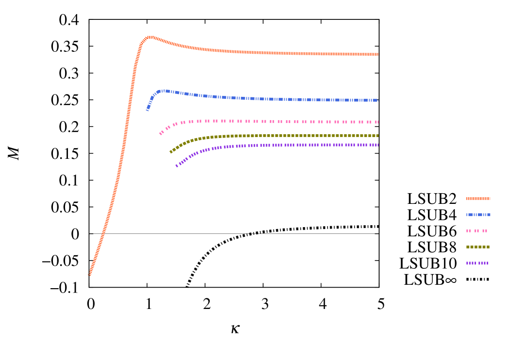
Figure 9: (Color online) CCM LSUB$n$ results for the GS magnetic order parameter, $M$, versus the frustration parameter $\kappa\equiv J_{2}/J_{1}$, for the spin-1/2 $J_{1}$–$J_{2}$ chevron-square lattice model (with $J_{1}>0$), using (a) the Néel and spiral states of Fig. 1(a) and 1(b) respectively as model states with $n=\{2,4,6,8\}$, and (b) the row-striped state of Fig. 1(c) as model state with $n=\{2,4,6,8,10\}$. In each case we show the extrapolated LSUB$\infty$ result using the data sets shown and the respective extrapolation formula of Eq. (9) and (10) respectively.

It is interesting to note that while the spiral state has lower energy than the row-striped state for all values ($\kappa<5$) of the frustration parameter shown at the lowest LSUB2 level of approximation, there is a crossover point above which the row-striped state lies lower in energy than the spiral state for each of the higher LSUB4 and LSUB6 levels of approximation. This is also true at the LSUB8 level, but the crossover point is now rather close to the point ($\kappa\approx 2.2$) at which the corresponding LSUB8 solution for the spiral state becomes unstable. The crossover point for the extrapolated results clearly shows some (relatively small) sensitivity with respect to which set of LSUB$n$ results is used to perform the extrapolation. In view of the instability of the spiral (LSUB8) results in the relevant range, our best estimate undoubtedly comes from using the data set $n=\{2,4,6\}$. This gives an energy crossover at $\kappa\approx 1.83$, above which the spiral state ceases to be the lowest-energy solution. This value is itself in remarkably good agreement with our estimate above for the (termination) point at $\kappa\approx 1.5$, above which the row-striped state is itself stable. Indications so far thus provide reasonably compelling evidence for a second QCP at a value $\kappa_{c_{2}}\approx 1.7(3)$, above which the spiral state ceases to be the stable GS.

In order to shed more light on this transition we now present our corresponding CCM results for the magnetic order parameter, $M$, defined to be the average local on-site magnetization. In Fig. 9(a) we show LSUB$n$ results for the Néel and spiral states as CCM model states with $n\leq 8$. Note that for the Néel state we also have LSUB10 results, not shown on the figure since we do not have corresponding LSUB10 results for the spiral state. Once again, it is clear that the LSUB8 results for the spiral state behave rather differently than the LSUB$n$ results with $n\leq 6$ in the region $\kappa>1$ as the instability around $\kappa\approx 2.2$ is approached. We also show in Fig. 9(a) our extrapolated LSUB$\infty$ result using Eq. (9) and the data set $n=\{2,4,6,8\}$. Once again, the overall accuracy of our results may be gauged by examining the two special cases of the pure isotropic HAF with NN interactions only on the square lattice ($\kappa=0$) and the triangular lattice ($\kappa=1$).

For the square lattice we find $M(\kappa=0)=0.3087$ using Eq. (9) with LSUB$n$ results for $n=\{4,6,8\}$ and $M(\kappa=0)=0.3074$ from $n=\{4,6,8,10\}$. These values are again in excellent agreement with the corresponding results $M(\kappa=0)=0.3070(3)$ from a large-scale QMC simulation,Sa:1997 and $M(\kappa=0)=0.307(1)$ from a linked-cluster SE calculation,Zh:1991 Similarly, for the triangular lattice we find $M(\kappa=1)=0.2219$ using Eq. (9) with LSUB$n$ results for $n=\{2,4,6,8\}$ and $M(\kappa=1)=0.1893$ from $n=\{4,6,8\}$. Again, we are in excellent agreement with other values $M(\kappa=1)=0.205(10)$ from a fixed-node QMC simulation,Ca:1999 , and $M(\kappa=1)=0.19(2)$ from a linked-cluster SE calculation.Zheng:2006

Figure 9(a) is completely consistent with the result that the magnetic order parameter $M\rightarrow 0$ at the critical point $\kappa=\kappa_{c_{1}}$ where the collinear Néel order for $\kappa<\kappa_{c_{1}}$ yields to the noncollinear spiral order. Our best estimate for $\kappa_{c_{1}}$, based on the results for $M$, is $\kappa_{c_{1}}=0.72(1)$, where the error is estimated from a sensitivity analysis with respect to which LSUB$n$ results are used in the extrapolation. There is also definite evidence from Fig. 9(a) that in the spiral regime ($\kappa>\kappa_{c_{1}}$), the spiral order parameter $M$ again becomes zero (or very close to zero) at a second critical value, $\kappa_{c_{2}}\approx 1.4$, which we discuss in more detail later.

Corresponding CCM LSUB$n$ results for the magnetic order parameter, $M$, for the row-striped state are shown in Fig. 9(b) with $n=\{2,4,6,8,10\}$. In this highly frustrated regime, if we fit our results to a form $M(n)=m_{0}+m_{1}n^{-\nu}$, as in Eq. (11), we find that the fitted value of the exponent $\nu$ turns out to be very close to 0.5 over almost the entire range of values of $\kappa$, independent of which LSUB$n$ data set is used for the fit. Hence, in this case it is appropriate to use the extrapolation scheme of Eq. (10), and in Fig. 9(b) we use the data set $n=\{2,4,6,8\}$ for illustration purposes and compatibility with Fig. 9(a). What is most striking about the extrapolated result is that $M$ appears to be essentially zero (or less than zero, and hence unphysical) over the entire regime in which the row-striped state exists as a candidate for the stable GS phase. In Fig. 10 we present various extrapolations of our CCM LSUB$n$ data, from which we observe their relative insensitivity to the choice of data set.

Figure 10: (Color online) Various extrapolated CCM results for the GS magnetic order parameter, $M$, versus the frustration parameter $\kappa\equiv J_{2}/J_{1}$, based on the Néel (left curves) and spiral (central curves) model states and the row-striped (right curves) model state, for the spin-1/2 $J_{1}$–$J_{2}$ chevron-square lattice model (with $J_{1}>0$). The curves LSUB$\infty(k)$ with $k=1,2,\cdots,5$ use the extrapolation scheme of Eq. (10) and LSUB$n$ data sets respectively: $k=1$, $n=\{2,4,6,8\}$; $k=2$, $n=\{4,6,8,10\}$; $k=3$, $n=\{6,8,10\}$, $k=4$, $n=\{4,6,8\}$, and $k=5$, $n=\{2,4,6\}$. The curves LSUB$\infty(k)$ with $k=6,7,8$ use the extrapolation scheme of Eq. (9) and LSUB$n$ data sets, respectively: $k=6$, $n=\{4,6,8,10\}$, for the Néel model state; and $k=7$, $n=\{2,4,6,8\}$, and $k=8$, $n=\{2,4,6\}$ for the spiral model state.

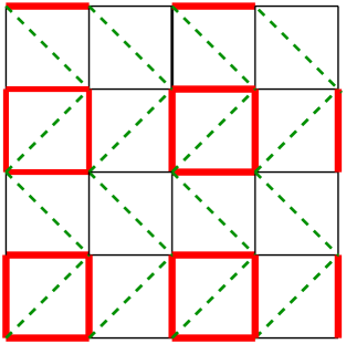
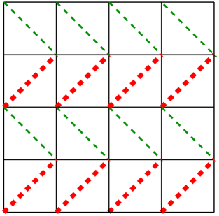
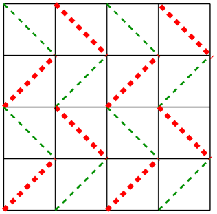
Figure 11: (Color online) The perturbations (fields), $F=\delta\,\hat{O}$, for the various forms of valence-bond crystal (VBC) susceptibility considered, namely: (a) plaquette (PVBC), $\chi_{p}$; (b) parallel-dimer ($\parallel$DVBC), $\chi_{{\rm d}_{\parallel}}$; and (c) perpendicular-dimer ($\perp$DVBC), $\chi_{{\rm d}_{\perp}}$. In case (a) the thick (red) and thin (black) solid lines correspond respectively to strengthened and weakened $J_{1}$ exchange couplings, where $\hat{O}_{\rm p}=\sum_{\langle i,j\rangle}a_{ij}\mathbf{s}_{i}\cdot\mathbf{s}_{j}$, and the sum runs over all NN bonds of the square lattice, with $a_{ij}=+1$ and $-1$ for thick (red) and thin (black) solid lines respectively, as shown. In cases (b) and (c) the thick (red) and thin (green) dashed lines correspond respectively to strengthened and weakened $J_{2}$ exchange couplings, and $\hat{O}_{{\rm d}}=\sum_{\langle\langle i,k\rangle\rangle}a_{ik}\mathbf{s}_{i}\cdot\mathbf{s}_{k}$, and the sum runs over the diagonal bonds of the chevron-square lattice, with $a_{ik}=+1$ and $-1$ for thick (red) and thin (green) dashed lines respectively, as shown in each case.

All of our results so far are consistent with the interpretation that the spiral state exists as the stable GS phase only in a regime $\kappa_{c_{1}}<\kappa<\kappa_{c_{2}}$, where $\kappa_{c_{2}}\approx 1.7(5)$. However, the estimates so far for $\kappa_{c_{2}}$ are based on the energy crossing point between the spiral and row-striped states, the termination points for the LSUB$n$ row-striped results, and the magnetic order parameter results for the row-striped state. Nevertheless, the latter results also indicate that, since $M\approx 0$ everywhere that the row-striped solution exists as a real solution, the row-striped state itself is actually never realized as the stable GS phase.

In order to obtain more information about the stable GS phase that the system actually enters after the melting of spiral order at $\kappa_{c_{2}}$ we now investigate its susceptibility to various forms of valence-bond crystalline (VBC) orders. In particular, we consider the plaquette valence-bond crystalline (PVBC) order illustrated in Fig. 11(a) and two forms of dimer valence-bond crystalline (DVBC) order illustrated in Figs. 11(b) and (c), respectively, which we refer to henceforth as parallel ($\parallel$DVBC) and perpendicular ($\perp$DVBC) forms. In each case we consider the response of the system to a corresponding field operator, $F=\delta\,\hat{O}$, which is added to the Hamiltonian of Eq. (1) (and see, e.g., Ref. Darradi:2008_J1J2mod, ). The corresponding operators $\hat{O}_{\rm p}$, $\hat{O}_{{\rm d}_{\parallel}}$, and $\hat{O}_{{\rm d}_{\perp}}$ for PVBC, $\parallel$DVBC, and $\perp$DVBC order are shown graphically in Fig. 11 and defined explicitly in the caption. For each form of VBC order considered, we then calculate the perturbed energy per site, $e(\delta)\equiv E(\delta)/N$, for the modified Hamiltonian $H+F$, at various LSUB$n$ levels of approximation, using the Néel and row-striped states as CCM model states. The corresponding susceptibility,

$$\chi\equiv-\left.(\partial^{2}{e(\delta)})/(\partial{\delta}^{2})\right|_{\delta=0}\,,$$ (12)

is then calculated. Clearly the phase corresponding to the model state used becomes unstable against the specified form of VBC order when the corresponding extrapolated inverse susceptibility, $\chi^{-1}_{d}$, goes to zero.

The most direct and most unbiased way to extrapolate the results is to use the LSUB$n$ scheme for the perturbed energy

$$e^{(n)}(\delta)=e_{0}(\delta)+e_{1}(\delta)n^{-\nu},$$ (13)

where the exponent $\nu$ is also a fitting parameter. Generally, as we discuss below, the fitted value of $\nu$ is close to the value 2, as expected from our standard energy extrapolation scheme of Eq. (8), over most of the range of values of $\kappa$ pertaining to the model state used, except very near any corresponding termination point for the given state, where $\nu$ then falls sharply. Alternatively, we have also found previouslyFarnell:2011 that our LSUB$n$ values $\chi(n)$ may often themselves be directly extrapolated very accurately using the same scheme as in Eq. (8) for the GS energy, viz., $\chi(n)=d_{0}+d_{1}n^{-2}+d_{2}n^{-4}$, at least in regions not close to a divergence of $\chi$. We saw similarlyFarnell:2011 that a corresponding extrapolation of the inverse susceptibility,

$$\chi^{-1}(n)=x_{0}+x_{1}n^{-2}+x_{2}n^{-4}\,,$$ (14)

also often gives consistent results that agree closely with those from the corresponding above extrapolation of $\chi$ itself, except again in regions close to where $\chi^{-1}\rightarrow 0$. However, since we shall specifically be interested in some cases here in precisely such regions over an extended range of values of the frustration parameter $\kappa$, we also use the fitting function

$$\chi^{-1}(n)=y_{0}+y_{1}n^{-\nu}\,,$$ (15)

with an exponent $\nu$ that is itself a fitting parameter, on appropriate occasions.

We first present results in Fig. 12 for the inverse plaquette susceptibility, $\chi^{-1}_{{\rm p}}$, pertaining to the PVBC ordering illustrated in Fig. 11(a).

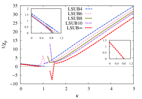
Figure 12: (Color online) CCM LSUB$n$ results for the inverse plaquette susceptibility, $1/\chi_{{\rm p}}$, appropriate to the PVBC ordering of Fig. 11(a), versus the frustration parameter $\kappa\equiv J_{2}/J_{1}$, using the Néel (left curves) and row-striped (right curves) states as model states for the spin-1/2 $J_{1}$–$J_{2}$ Heisenberg antiferromagnet on the chevron-square lattice (with $J_{1}>0$). For both model states we show the LSUB$n$ results with $n=\{4,6,8,10\}$, plus the corresponding extrapolated results LSUB$\infty$ using this data set with the extrapolation scheme of Eq. (13).

We show explicitly the LSUB$n$ results with $n=\{4,6,8,10\}$ based on both the Néel and row-striped states as CCM model states, together with the corresponding LSUB$\infty$ extrapolations using Eq. (13) with these data sets. As noted above, the fitted value of the exponent $\nu$ in Eq. (13) is very close to 2 except in very narrow regions close to $\kappa_{c_{1}}$ on the Néel side and close to $\kappa_{c_{2}}$ on the row-striped side. It is interesting to note that the Néel phase has a high susceptibility to PVBC ordering, although $\chi^{-1}_{{\rm p}}\rightarrow 0$ only at a single value which is very close to our previous best estimate for $\kappa_{c_{1}}$. While the row-striped state, on the other hand, is clearly much less susceptible to PVBC ordering, the corresponding LSUB$\infty$ estimate for $\chi^{-1}_{{\rm p}}$ again becomes very close to zero at a value $\kappa_{c_{2}}\approx 1.4$, which is again compatible with our previous estimates for $\kappa_{c_{2}}$. Presumably, if we were also to perform calculations for $\chi^{-1}_{{\rm p}}$ for the spiral phase, it too would be nonzero (and positive) everywhere except at the values $\kappa_{c_{1}}$ and $\kappa_{c_{2}}$. However, such calculations for the spiral phase are computationally very expensive, and as noted previously can be performed only for relatively lower LSUB$n$ orders of approximation. Even for the collinear row-striped state the number $N_{f}$ of fundamental spin configurations included in our CCM calculation at the LSUB10 level is 2160176.

While the results shown in Fig. 12 corroborate our previous estimates for the QCPs at $\kappa_{c_{1}}$ (at which Néel order yields to spiral order) and $\kappa_{c_{2}}$ (at which spiral order ceases), they essentially add nothing new. Thus, it is clear that the PVBC state cannot be the stable GS phase for any range of values $\kappa>\kappa_{c_{2}}$, since $\chi^{-1}_{{\rm p}}$ does not vanish over any finite range in this regime. The fact that $\chi^{-1}_{{\rm p}}$ vanishes at individual points (viz., $\kappa_{c_{1}}$ and $\kappa_{c_{2}}$ here) is simply a reflection of these being actual QCPs. Thus, at a QCP we expect that the system will indeed become infinitely susceptible to all forms of ordering (or, at least, those which are compatible with the symmetries of the actual and trial states).

We now turn our attention to the two DVBC states of Figs. 11(b) and (c) as possible GS phases for $\kappa>\kappa_{c_{2}}$. Firstly, since our results for the inverse susceptibility, $1/\chi_{{\rm d}_{\perp}}$, for $\perp$DVBC ordering are qualitatively very similar to those shown in Fig. 12 for PVBC ordering, we do not show them. Again, we find that using the Néel model state $\chi^{-1}_{{\rm d}_{\perp}}$ vanishes at a single point, which is itself completely compatible with our previous estimates for $\kappa_{c_{1}}$, and using the row-striped model state $\chi^{-1}_{{\rm d}_{\perp}}$ vanishes at a single point compatible with our previous estimates for $\kappa_{c_{2}}$. Thus, again, the $\perp$DVBC state is excluded as a stable GS phase in any range $\kappa>\kappa_{c_{2}}$.

By contrast, our results for the inverse susceptibility, $1/\chi_{{\rm d}_{\parallel}}$, for $\parallel$DVBC ordering, shown in Fig. 13(a) are qualitatively quite different in the regime $\kappa>\kappa_{c_{2}}$. In the inset to Fig. 13(a) we show the raw LSUB$n$ results for $n=\{2,4,6,8,10\}$ using both the Néel and row-striped states as CCM model states, while in the main figure we show several LSUB$\infty$ extrapolations based on both Eqs. (13) and (15), and using various LSUB$n$ data sets for the fitting procedure.

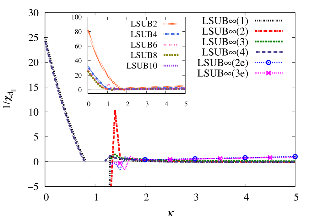
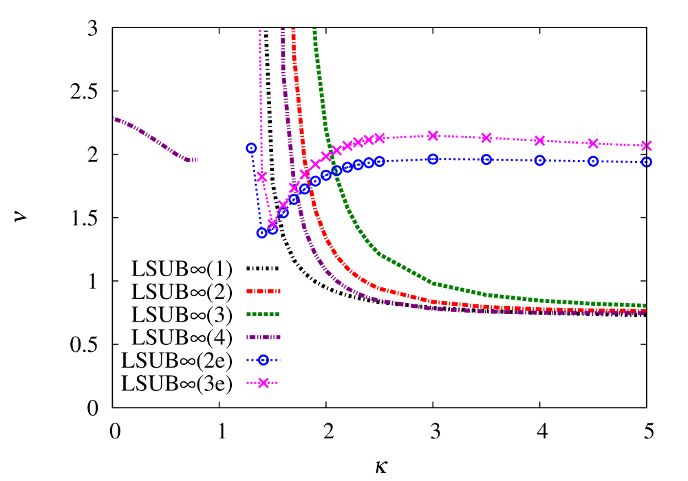
Figure 13: (Color online) (a) CCM results for the inverse parallel-dimer susceptibility, $1/\chi_{d_{\parallel}}$, appropriate to the $\parallel$DVBC ordering of Fig. 11(b), versus the frustration parameter $\kappa\equiv J_{2}/J_{1}$, using the Néel (left curves) and row-striped (right curves) states of Figs. 1(a) and 1(c), respectively, as model states for the spin-1/2 $J_{1}$–$J_{2}$ Heisenberg antiferromagnet on the chevron-square lattice ($J_{1}>0$). For both model states we show the LSUB$n$ results with $n=\{2,4,6,8,10\}$ in the inset, while the main figure shows various LSUB$\infty$ extrapolations. The curves LSUB$\infty(k)$ (without symbols attached) with $k=1,\cdots,4$ use the extrapolation scheme of Eq. (15), while the curves LSUB$\infty(k{\rm e})$ (with symbols attached) with $k=2,3$ use the extrapolation scheme of Eq. (13), in both cases using the respectively LSUB$n$ data sets: $k=1$, $n=\{2,4,6,8\}$; $k=2$, $n=\{4,6,8,10\}$; $k=3$, $n=\{6,8,10\}$; and $k=4$, $n=\{4,6,8\}$. (b) The respective fitted values of the exponent $\nu$ in the extrapolation schemes of Eqs. (13) and (15), for the same fits as shown in subfigure (a) to the left.

In Fig. 13(b) we also show the fitted values for the exponent $\nu$ in the corresponding extrapolation schemes.

In the first place we find that on the Néel side all of the extrapolations yield almost identical results, with $\chi^{-1}_{d_{\parallel}}\rightarrow 0$ at values $\kappa\rightarrow\kappa_{c_{1}}$, which are in agreement with all previous estimates. Secondly, however, we now see from Fig. 13(a) that using the row-striped state as CCM model state, all of our extrapolations yield the result that $1/\chi_{{\rm d}_{\parallel}}$ is zero (or very close to zero) for all values $\kappa>\kappa_{{c_{2}}}\approx 1.5$. We thus now have very strong evidence indeed that for $\kappa>\kappa_{c_{2}}$, the GS spiral ordering present for $\kappa_{c_{1}}<\kappa<\kappa_{c_{2}}$ gives way to $\parallel$DVBC ordering as the stable GS configuration.

Figure 13(b) shows that when $\chi_{{\rm d}_{\parallel}}$ is calculated using Eq. (13) as the extrapolation scheme the fitted exponent $\nu$ is very close to the expected value 2 for a very wide range of values of $\kappa$, as in our standard GS energy scheme of Eq. (8), except for values of $\kappa$ close to $\kappa_{c_{2}}$, where it drops. In practice we calculate the second derivative of $e(\delta)$ in Eq. (12) numerically using values $\delta=0\,,\pm d$, typically with $d=0.001$, and the value of $\nu$ plotted in Fig. 13(b) is essentially identical for these three values of $\delta$ used. By contrast, when $1/\chi_{{\rm d}_{\parallel}}$ is calculated using Eq. (15), the fitted exponent $\nu$ is seen to lie very close to the value 0.75 for a very wide range of values of $\kappa$, except for values close to $\kappa_{c_{2}}$ where it rises rapidly. Interestingly, this same value of 0.75 was also observed previously for the spin-1/2 $J_{1}$–$J_{2}$ Heisenberg antiferromagnet on the 2D checkerboard lattice (viz., the APP model),Bishop:2012_checkerboard when using a similar state as CCM model state in a region where the order parameter for that state was zero everywhere, and where a corresponding DVBC state also provided the stable GS configuration.

V SUMMARY

We have investigated the $T=0$ GS phase diagram of an $s=\frac{1}{2}$ $J_{1}$–$J_{2}$ HAF on a chevron-square lattice, the classical ($s\rightarrow\infty$) version of which has only two GS phases, viz., a Néel phase for $J_{2}/J_{1}\equiv\kappa<\kappa_{{\rm cl}}=\frac{1}{2}$, and a spirally-ordered phase for $\kappa>\kappa_{{\rm cl}}$. The model interpolates continuously between 2D HAFs on the square ($\kappa=0$) and triangular ($\kappa=1$) lattices, and also extrapolates in the $\kappa\rightarrow\infty$ limit to uncoupled 1D HAF chains.

We found, as expected, that the quantum fluctuations present in the $s=\frac{1}{2}$ model tend to stabilize the collinear Néel-ordered state, which is well established as the GS phase for the square-lattice HAF, to larger values of the frustration parameter $\kappa$ than in the classical case. We found a first QCP at $\kappa=\kappa_{c_{1}}\approx 0.72(1)$ at which the Néel order gives way to spiral order. The pitch angle $\phi$ of the spiral phase (that measures the deviation from Néel order corresponding to $\phi=0$) was found to increase markedly more rapidly as $\kappa$ is increased beyond $\kappa_{c_{1}}$ than in the classical version as $\kappa$ is increased beyond $\kappa_{{\rm cl}}$.

Although the transition at $\kappa=\kappa_{c_{1}}$ appears still to be a continuous (second-order) one, just as for the classical model at $\kappa=\kappa_{{\rm cl}}$, we cannot from our results rule out a weakly first-order transition at which the pitch angle $\phi$ undergoes a discontinuous jump from a value of zero (Néel order) for $\kappa<\kappa_{c_{1}}$ to a nonzero value (spiral order) infinitesimally above $\kappa_{c_{1}}$. The angle $\phi$ becomes exactly $60^{\circ}$ at all levels of CCM LSUB$n$ approximation at $\kappa=1$, corresponding to the exact three-sublattice relative $120^{\circ}$ spin ordering that is well established as the GS phase for the spin-1/2 triangular-lattice HAF.

At still higher values of the frustration parameter, $\kappa>1$, we found that the pitch angle $\phi$ of the $s=\frac{1}{2}$ model approaches the limiting value of $90^{\circ}$ (which corresponds to Néel AFM ordering along the 1D chevron chains of $J_{2}$ bonds) much faster than in the classical ($s\rightarrow\infty$) model. In turn this led us to consider other possible collinear phases in this regime, which never form the stable GS phase in the classical case, except in the precise $\kappa\rightarrow\infty$ limit, but which comprise an infinitely degenerate family of states corresponding to Néel ordering along the 1D chevron chains. We found that the order by disorder mechanism distinguishes one such state from the rest, so that quantum fluctuations in the $s=\frac{1}{2}$ case favor it to lie lowest in energy. Furthermore, above some value of the frustration parameter, $\kappa>\kappa_{c_{2}}$, this state was seen to become lower in energy too than the spiral state for the $s=\frac{1}{2}$ model. However, when we then calculated its magnetic order parameter, we found it to be zero, within very small numerical error bars, everywhere.

We were thus led to the conclusion that the spiral order in the $s=\frac{1}{2}$ model does not persist for all values $\kappa>\kappa_{c_{1}}$, but only for a finite range $\kappa_{c_{1}}<\kappa<\kappa_{c_{2}}$, unlike in the classical model where it persists for all values $\kappa>\kappa_{{\rm cl}}$. Instead, we found again that the magnetic order parameter of the spiral phase seems to vanish for values of $\kappa$ above a certain critical value, which is itself consistent within small errors bars with the energy crossing point of the spiral state with the nonclassical collinear state mentioned.

Since this latter collinear state itself has a vanishing magnetic order parameter in the same region, as already noted, it must itself yield to a state with different ordering. By comparison with other related depleted $J_{1}$–$J_{2}$ models, we were led to consider that this collinear state might be susceptible to some form of VBC ordering, and we therefore calculated its susceptibility to both PVBC ordering and two forms of DVBC ordering. From among these we found unequivocal evidence that there is a second QCP in the $s=\frac{1}{2}$ model at a value $\kappa=\kappa_{c_{2}}\approx 1.5(1)$ at which the spiral order present for $\kappa_{c_{1}}<\kappa<\kappa_{c_{2}}$ melts and gives way for values $\kappa>\kappa_{c_{2}}$ to a parallel-dimer VBC ($\parallel$DVBC) order.

In conclusion, the $J_{1}$–$J_{2}$ HAF on the chevron-square lattice has been found to provide a rich GS phase diagram for the extreme quantum case, $s=\frac{1}{2}$. It would certainly be interesting, therefore, both to confirm our results using other theoretical methods and to examine the corresponding $s=1$ version of the model.

References

- (1) Quantum Magnetism, Lecture Notes in Physics Vol. 645, edited by U. Schollwöck, J. Richter, D. J. J. Farnell, and R. F. Bishop (Springer-Verlag, Berlin, 2004).
- (2) G. Misguich and C. Lhuillier, in Frustrated Spin Systems, edited by H. T. Diep (World Scientific, Singapore, 2005), p. 229.
- (3) S. Sachdev and B. Keimer, Phys. Today 64(2), 29 (2011).
- (4) J. Villain, J. Phys. (France) 38, 385 (1977); J. Villain, R. Bidaux, J. P. Carton, and R. Conte, ibid. 41, 1263 (1980).
- (5) R. R. P. Singh, O. A. Starykh, and P. J. Freitas, J. Appl. Phys. 83, 7387 (1998).
- (6) S. E. Palmer and J. T. Chalker, Phys. Rev. B 64, 094412 (2001).
- (7) W. Brenig and A. Honecker, Phys. Rev. B 65, 140407(R) (2002).
- (8) B. Canals, Phys. Rev. B 65, 184408 (2002).
- (9) O. A. Starykh, R. R. P. Singh, and G. C. Levine, Phys. Rev. Lett. 88, 167203 (2002).
- (10) P. Sindzingre, J.-B. Fouet, and C. Lhuillier, Phys. Rev. B 66, 174424 (2002).
- (11) J.-B. Fouet, M. Mambrini, P. Sindzingre, and C. Lhuillier, Phys. Rev. B 67, 054411 (2003).
- (12) E. Berg, E. Altman, and A. Auerbach, Phys. Rev. Lett. 90, 147204 (2003).
- (13) O. Tchernyshyov, O. A. Starykh, R. Moessner, and A. G. Abanov, Phys. Rev. B 68, 144422 (2003).
- (14) R. Moessner, O. Tchernyshyov, and S. L. Sondhi, J. Stat. Phys. 116, 755 (2004).
- (15) M. Hermele, M. P. A. Fisher, and L. Balents, Phys. Rev. B 69, 064404 (2004).
- (16) W. Brenig and M. Grzeschik, Phys. Rev. B 69, 064420 (2004).
- (17) J. S. Bernier, C. H. Chung, Y. B. Kim, and S. Sachdev, Phys. Rev. B 69, 214427 (2004).
- (18) O. A. Starykh, A. Furusaki, and L. Balents, Phys. Rev. B 72, 094416 (2005).
- (19) H.-J. Schmidt, J. Richter, and R. Moessner, J. Phys. A: Math. Gen. 39, 10673 (2006).
- (20) M. Arlego and W. Brenig, Phys. Rev. B 75, 024409 (2007); ibid. 80, 099902(E) (2009).
- (21) S. Moukouri, Phys. Rev. B 77, 052408 (2008).
- (22) Y.-H. Chan, Y.-J. Han, and L.-M. Duan, Phys. Rev. B 84, 224407 (2011).
- (23) R. F. Bishop, P. H. Y. Li, D. J. J. Farnell, J. Richter, and C. E. Campbell, Phys. Rev. B 85, 205122 (2012).
- (24) V. J. Emery, E. Fradkin, S. A. Kivelson, and T. C. Lubensky, Phys. Rev. Lett. 85, 2160 (2000).
- (25) R. Mukhopadhyay, C. L. Kane, and T. C. Lubensky, Phys. Rev. B 64, 045120 (2001).
- (26) A. Vishwanath and D. Carpentier, Phys. Rev. Lett. 86, 676 (2001).
- (27) R. F. Bishop and H. G. Kümmel, Phys. Today 40(3), 52 (1987).
- (28) J. S. Arponen and R. F. Bishop, Ann. Phys. (N.Y.) 207, 171 (1991).
- (29) R. F. Bishop, Theor. Chim. Acta 80, 95 (1991).
- (30) R. F. Bishop, in Microscopic Quantum Many-Body Theories and Their Applications, Lecture Notes in Physics Vol. 510, edited by J. Navarro and A. Polls, (Springer-Verlag, Berlin, 1998), p. 1.
- (31) D. J. J. Farnell and R. F. Bishop, in Quantum Magnetism, Lecture Notes in Physics Vol. 645, edited by U. Schollwöck, J. Richter, D. J. J. Farnell, and R. F. Bishop, (Springer-Verlag, Berlin, 2004), p. 307.
- (32) R. F. Bishop, J. B. Parkinson, and Yang Xian, Phys. Rev. B 44, 9425 (1991).
- (33) C. Zeng, D. J. J. Farnell, and R. F. Bishop, J. Stat. Phys. 90, 327 (1998).
- (34) S. E. Krüger, J. Richter, J. Schulenburg, D. J. J. Farnell, and R. F. Bishop, Phys. Rev. B 61, 14607 (2000).
- (35) R. F. Bishop, D. J. J. Farnell, S.E. Krüger, J. B. Parkinson, J. Richter, and C. Zeng, J. Phys.: Condens. Matter 12, 6887 (2000).
- (36) D. J. J. Farnell, R. F. Bishop, and K. A. Gernoth, Phys. Rev. B 63, 220402(R) (2001).
- (37) R. Darradi, J. Richter, and D. J. J. Farnell, Phys. Rev. B 72, 104425 (2005).
- (38) R. Darradi, O. Derzhko, R. Zinke, J. Schulenburg, S. E. Krüger, and J. Richter, Phys. Rev. B 78, 214415 (2008).
- (39) D. Schmalfuß, R. Darradi, J. Richter, J. Schulenburg, and D. Ihle, Phys. Rev. Lett. 97, 157201 (2006).
- (40) R. F. Bishop, P. H. Y. Li, R. Darradi, and J. Richter, J. Phys.: Condens. Matter 20, 255251 (2008).
- (41) R. F. Bishop, P. H. Y. Li, R. Darradi, J. Schulenburg, and J. Richter, Phys. Rev. B 78, 054412 (2008).
- (42) R. F. Bishop, P. H. Y. Li, D. J. J. Farnell, and C. E. Campbell, Phys. Rev. B 79, 174405 (2009).
- (43) J. Richter, R. Darradi, J. Schulenburg, D.J.J. Farnell, and H. Rosner, Phys. Rev. B 81, 174429 (2010).
- (44) R. F. Bishop, P. H. Y. Li, D. J. J. Farnell, and C. E. Campbell, Phys. Rev. B 82, 024416 (2010).
- (45) J. Reuther, P. Wölfle, R. Darradi, W. Brenig, M. Arlego, and J. Richter, Phys. Rev. B 83, 064416 (2011).
- (46) D. J. J. Farnell, R. F. Bishop, P. H. Y. Li, J. Richter, and C. E. Campbell, Phys. Rev. B 84, 012403 (2011).
- (47) O. Götze, D. J. J. Farnell, R. F. Bishop, P. H. Y. Li, and J. Richter, Phys. Rev. B 84, 224428 (2011).
- (48) P. H. Y. Li, R. F. Bishop, D. J. J. Farnell, and C. E. Campbell, Phys. Rev. B 86, 144404 (2012).
- (49) P. H. Y. Li, R. F. Bishop, C. E. Campbell, D. J. J. Farnell, O. Götze and J. Richter, Phys. Rev. B 86, 214403 (2012).
- (50) J. Struck, C. Ölschäger, R. Le Targat, P. Soltan-Panahi, A. Eckardt, M. Lewenstein, P. Windpassinger, and K. Sengstock, Science 333, 996 (2011).
- (51) H. Bethe, Z. Phys. 71, 205 (1931).
- (52) We use the program package CCCM of D. J. J. Farnell and J. Schulenburg, see http://www-e.uni-magdeburg.de/jschulen/ccm/index.html.
- (53) Zheng Weihong, J. Oitmaa, and C. J. Hamer, Phy. Rev. B 43, 8321 (1991).
- (54) A. W. Sandvik, Phys. Rev. B 56, 11678 (1997).
- (55) W. Marshall, Proc. R. Soc. London, Ser. A 232, 48 (1955).
- (56) W. Zheng, J. O. Fjaerestad, R. R. P. Singh, R. H. McKenzie, and R. Coldea, Phys. Rev. B 74, 224420 (2006).
- (57) L. Capriotti, A. E. Trumper, and S. Sorella, Phys. Rev. Lett. 82, 3899 (1999).
- (58) L. Hulthén, Ark. Mat. Astron. Fys. A 26 (No. 11), 1 (1938); R. Orbach, Phy. Rev. 112, 309 (1958); C. N. Yang and C. P. Yang, ibid. 150, 321 (1966); 150, 327 (1966); R. J. Baxter, J. Stat. Phys. 9, 145 (1973).