$\mathcal{P}\mathcal{T}$-Symmetric Dimer of Coupled Nonlinear Oscillators

Abstract

We provide a systematic analysis of a prototypical nonlinear oscillator system respecting $\mathcal{P}\mathcal{T}$-symmetry i.e., one of them has gain and the other an equal and opposite amount of loss. Starting from the linear limit of the system, we extend considerations to the nonlinear case for both soft and hard cubic nonlinearities identifying symmetric and anti-symmetric breather solutions, as well as symmetry breaking variants thereof. We propose a reduction of the system to a Schrödinger type $\mathcal{P}\mathcal{T}$-symmetric dimer, whose detailed earlier understanding can explain many of the phenomena observed herein, including the $\mathcal{P}\mathcal{T}$ phase transition. Nevertheless, there are also significant parametric as well as phenomenological potential differences between the two models and we discuss where these arise and where they are most pronounced. Finally, we also provide examples of the evolution dynamics of the different states in their regimes of instability.

I Introduction

The topic of Parity-Time ($\mathcal{PT}$) symmetry and its relevance to physical applications on the one hand, as well as its mathematical structure on the other have drawn considerable attention both from the physics and the mathematics communities. Originally, this theme was proposed by C. Bender and co-workers as an additional possibility for operators associated with real measurable quantities within linear quantum mechanics R1 ; R2 ; R221 . However, one of the major milestones (and a principal thrust of recent activity) regarding the physical/experimental realizability of the corresponding Hamiltonians stemmed from progress in optics both at the theoretical ziad ; Muga and at the experimental salamo ; dncnat level. In particular, the realization that in optics, the ubiquitous loss can be counter-acted by an overwhelming gain, in order to create a $\mathcal{PT}$-symmetric setup e.g. in a waveguide dimer dncnat paved the way for numerous developments especially so at the level of nonlinear systems, as several researchers studied nonlinear stationary states, stability and dynamics of few site configurations Dmitriev ; Li ; Guenter ; Ramezani ; suchkov ; Sukhorukov ; ZK as well as of infinite lattices Pelin1 ; Sukh ; zheng .

Interestingly, most of this nonlinear activity has been centered around Schrödinger type systems and for good reason, since the original proposal by Bender involved quantum mechanical settings, where this is natural and in addition the optics proposal was placed chiefly on a similar footing (i.e., the Schrödinger model as paraxial approximation to the Maxwell equations). Nevertheless, there have been a few notable exceptions where nonlinear oscillator models (involving second order differential equations in time) have been considered. Perhaps the most relevant example, also for the considerations presented herein, has involved the realization of $\mathcal{P}\mathcal{T}$-symmetric dimers in the context of electrical circuits; for the first work in this context, see tsampas , while that and follow-up activity has recently been summarized in a review tsamp_rev . Chiefly, the experimental considerations of these works focused on the linear variant of the gain-loss oscillator system. More recently, nonlinear variants of $\mathcal{P}\mathcal{T}$-symmetric dimers in the form of a chain have been proposed in the context of magnetic metamaterials and in particular for systems consisting of split-ring resonators tsironis . The latter setting, while nonlinear is also far more complex (involving external drive and nonlinear couplings between adjacent sites) and hence was tackled for the nonlinear model chiefly at the level of direct numerical simulations.

Our aim herein is to provide a simple, prototypical nonlinear model, whose linear analog is effectively the one used in the experimental investigations of tsampas . Yet, the nonlinear structure is such that it allows to obtain a detailed numerical and even considerable analytical insights on the phenomenology of such a nonlinear $\mathcal{P}\mathcal{T}$-symmetric oscillator dimer. In particular, after formulating and briefly analyzing the linear $\mathcal{P}\mathcal{T}$-symmetric coupled oscillator model, we incorporate into it a local cubic nonlinearity (which can, in general, be of soft or hard form i.e., bearing a prefactor of either sign). This type of potential, especially in its bistable form, is well known to be a canonical example of relevance to numerous physical settings, including (but not limited to) phase transitions, superconductivity, field theories and high energy/particle physics; see e.g. campbell and the review belova , as well as references therein. For the resulting $\mathcal{P}\mathcal{T}$-symmetric, coupled nonlinear oscillator model, we provide a detailed analysis of the existence and stability of breathing (i.e., time-periodic) states in the system. We focus particularly on symmetric and anti-symmetric such states that arise from the linear limit of the problem. We observe that symmetry-breaking type bifurcations can arise for both the symmetric and anti-symmetric branches and eventually highlight a nonlinear analog of $\mathcal{P}\mathcal{T}$ phase transition whereby the two branches terminate hand-in-hand in a saddle-center bifurcation.

To provide an analytical insight into the above results, we use the Rotating Wave Approximation (RWA) which approximates the system by the corresponding nonlinear Schrödinger type $\mathcal{P}\mathcal{T}$-symmetric dimer for which everything can be solved analytically, including the stationary states, the symmetry breaking bifurcations and even the full dynamics Ramezani ; Li ; Pelinov ; hadiadd . A direct comparison of the RWA-derived Schrödinger dimer reveals natural similarities, but also significant differences between the two models. For instance, in the way of similarities, both models bear symmetric and anti-symmetric branches of solutions, both models bear principal symmetry-breaking (of the symmetric branch in the soft –attractive– nonlinearity and of the anti-symmetric one for the hard –repulsive– nonlinearity) bifurcations, and both have $\mathcal{P}\mathcal{T}$ phase transitions, involving the collision and disappearance of these two branches. On the other hand, in terms of substantial differences, it is naturally expected that for soft nonlinearities, the oscillator model can escape the potential well (and hence have collapse features) even when the Schrödinger model cannot; see for a detailed recent discussion of such features in the Hamiltonian limit the work of escape . More importantly for our purposes, another significant difference is that it turns out that both branches, namely both the symmetric and the anti-symmetric one have destabilizing symmetry-breaking bifurcations, even though in the Schrödinger reduction, only one of the two branches (the symmetric for soft and the anti-symmetric for hard, as mentioned above) sustains such bifurcations. It should also be mentioned that after completing the examination of the prototypical time-periodic states and their Floquet theory based stability, we corroborate our bifurcation results by means of direct numerical simulations in order to explore the different dynamical evolution possibilities that arise in this system. These include among others the indefinite growth for the hard potential and the finite time blow up for the soft potential.

Our presentation of the two models and their similarities/differences proceeds as follows. In section II, we briefly discuss the underlying linear model and the prototypical nonlinear extension thereof. In section III, we discuss the numerical setup for analyzing the model and its solutions, while in section IV, we provide a means of theoretical analysis in the form of the rotating wave approximation. In section V, we present the numerical results, separating the cases of the soft and hard potential. Finally, in section VI, we summarize our findings and present our conclusions, as well as some directions for future study.

II Model equations and linear analysis

We consider the system motivated by recent experimental realizations in electrical circuits of the form:

$$\ddot{u} = -\omega_{0}^{2}u+sv+\gamma\dot{u},$$ (1)

$$\ddot{v} = -\omega_{0}^{2}v+su-\gamma\dot{v}.$$ (2)

Here, $\omega_{0}$ characterizes the internal oscillator at each mode; in the case of the electrical circuit model this is the oscillation of each of the charges within the dimer tsampas . The term proportional to $s$ reflects the coupling between the two elements in the dimer, while $\gamma$ is proportional to the amplification/resistance within the system.

One can try to identify the eigenvalues of the system by using $u=Ae^{i\Omega t}$ and $v=Be^{i\Omega t}$, but one obtains in this case a quadratic pencil for the relevant eigenvalue problem. It is thus easier to formulate this as a $4\times 4$ first order (linear) dynamical system according to:

$$\dot{u} = p,$$ (3)

$$\dot{p} = -u+\gamma p+sv,$$ (4)

$$\dot{v} = q,$$ (5)

$$\dot{q} = su-v-\gamma q,$$ (6)

(where $\omega_{0}$ has been rescaled without loss of generality to unity, and other quantities such as $s$ and $\gamma$ and time have been rescaled by $\omega_{0}^{2}$ -the first- and $\omega_{0}$ -the latter two-, respectively). We can then seek solutions of the form $u=Ae^{\lambda t}$, $p=Be^{\lambda t}$, $v=Ce^{\lambda t}$ and $q=De^{\lambda t}$, to obtain a first order eigenvalue problem which yields the following eigenvalues

$$\lambda=\pm\frac{\sqrt{-2+\gamma^{2}\pm\sqrt{4s^{2}-4\gamma^{2}+\gamma^{4}}}}{\sqrt{2}}.$$ (7)

These two pairs of imaginary (for small $\gamma$) eigenvalues will collide and give rise to a quartet for $\gamma>\gamma_{PT}$, where $\gamma_{PT}$ satisfies the condition:

$$\gamma^{4}-4\gamma^{2}+4s^{2}=0.$$ (8)

Hence Eq. (8) will define, at the linear level, the point of the so-called R1 ; R2 ; R221 $\mathcal{P}\mathcal{T}$ phase transition and of bifurcation into the complex plane.

Now, our main interest in what follows will be to examine a prototypical nonlinear variant of the problem which will be formulated as follows. In particular, we set up the form of the equations:

$$\ddot{u} = -u+sv+\gamma\dot{u}+\epsilon u^{3},$$ (9)

$$\ddot{v} = -v+su-\gamma\dot{v}+\epsilon v^{3}.$$ (10)

Here, in parallel to what is done in the $\mathcal{P}\mathcal{T}$-symmetric Schrödinger dimer typically dncnat ; Ramezani ; Li , we have added a cubic onsite nonlinearity on each one of the nodes. For $\epsilon>0$, this nonlinearity is soft, imposing a finite (maximal energy) height type of potential, enabling the possibility of indefinite growth by means of the escape scenario considered earlier e.g. in escape (see also references therein). On the other hand, for $\epsilon<0$, the nonlinearity is hard, and the potential is monostable bearing only the ground state at $0$ and no possibility for such finite time collapse (in the Hamiltonian analog of the model, only the potential for oscillations around the $0$ state exists in this case of the hard potential).

We now discuss the setup and numerical methods, as well as the type of diagnostics that we use for this system. In our description below, we follow an approach reminiscent of that in phason .

III Setup, Diagnostics and Numerical Methods

III.1 Existence of Periodic Orbit Solutions

In order to calculate periodic orbits in the $\mathcal{P}\mathcal{T}$ nonlinear oscillator dimer, we make use of a Fourier space implementation of the dynamical equations and continuations in frequency or gain/loss parameter are performed via a path-following (Newton-Raphson) method. Fourier space methods are based on the fact that the solutions are $T_{\mathrm{b}}$-periodic; for a detailed explanation of these methods, the reader is referred to Refs. AMM99 ; Marin ; Cuevas . The method has the advantage, among others, of providing an explicit, analytical form of the Jacobian. Thus, the solution for the two nodes can be expressed in terms of a truncated Fourier series expansion:

$$u(t)=\sum_{k=-k_{m}}^{k_{m}}y_{k}\exp(\mathrm{i}k\omega_{\mathrm{b}}t),\qquad v(t)=\sum_{k=-k_{m}}^{k_{m}}z_{k}\exp(\mathrm{i}k\omega_{\mathrm{b}}t),$$ (11)

with $k_{m}$ being the maximum of the absolute value of the running index $k$ in our Galerkin truncation of the full Fourier series solution. In the numerics, $k_{m}$ has been chosen as 21. After the introduction of (11), the dynamical equations (9)-(10) yield a set of $2\times(2k_{m}+1)$ nonlinear, coupled algebraic equations:

$$F_{k,1} \equiv -\omega_{\mathrm{b}}^{2}k^{2}y_{k}-\mathrm{i}\gamma\omega_{\mathrm{b}}ky_{k}+\mathcal{F}_{k}[V^{\prime}(u)]-sz_{k}=0,$$ (12)

$$F_{k,2} \equiv -\omega_{\mathrm{b}}^{2}k^{2}z_{k}+\mathrm{i}\gamma\omega_{\mathrm{b}}kz_{k}+\mathcal{F}_{k}[V^{\prime}(v)]-sy_{k}=0,$$ (13)

with $V^{\prime}(u)=u-\epsilon u^{3}$. Here, $\mathcal{F}_{k}$ denotes the Discrete Fourier Transform:

$$\mathcal{F}_{k}[V^{\prime}(u)]=\frac{1}{N}\sum_{n=-k_{m}}^{k_{m}}V^{\prime}\left(\sum_{p=-k_{m}}^{k_{m}}y_{p}\exp\left[\mathrm{i}\frac{2\pi pn}{N}\right]\right)\exp\left[-\mathrm{i}\frac{2\pi kn}{N}\right],$$ (14)

with $N=2k_{m}+1$. The procedure for $\mathcal{F}_{k}(v)$ is similar to the previous one. As $u(t)$ and $v(t)$ must be real functions, it implies that $y_{-k}=y^{*}_{k},\ z_{-k}=z^{*}_{k}$.

An important diagnostic quantity for probing the dependence of the solutions on parameters such as the gain/loss strength $\gamma$, or the oscillation frequency $\omega_{\mathrm{b}}$ is the averaged over a period energy, defined as:

$$<H>=\frac{1}{T}\int_{0}^{T}\ H(t)\,\mathrm{d}t,$$ (15)

with the Hamiltonian (of the case without gain/loss) being

$$H=\frac{\dot{u}^{2}+\dot{v}^{2}+u^{2}+v^{2}}{2}-\frac{\epsilon}{4}(u^{4}+v^{4})-suv,$$ (16)

and constituting a conserved quantity of the dynamics in the Hamiltonian limit of $\gamma=0$.

III.2 Linear stability equations

In order to study the spectral stability of periodic orbits, we introduce a small perturbation $\{\xi_{1},\xi_{2}\}$ to a given solution $\{u_{0},v_{0}\}$ of Eqs. (9)-(10) according to $u=u_{0}+\xi_{1}$, $v=v_{0}+\xi_{2}$. Then, the equations satisfied to first order in $\xi_{n}$ read:

$$\ddot{\xi}_{1}+V^{\prime\prime}(u_{0})\xi_{1}-\gamma\dot{\xi}_{1}-s\xi_{2} = 0,$$ (17)

$$\ddot{\xi}_{2}+V^{\prime\prime}(v_{0})\xi_{2}+\gamma\dot{\xi}_{2}-s\xi_{1} = 0,$$ (18)

or, in a more compact form: $\mathcal{N}(\{u(t),v(t)\})\xi=0\,$, where $\mathcal{N}(\{u(t),v(t)\})$ is the relevant linearization operator. In order to study the spectral (linear) stability analysis of the relevant solution, a Floquet analysis can be performed if there exists $T_{b}\in\mathbb{R}$ so that the map $\{u(0),v(0)\}\rightarrow\{u(T_{\mathrm{b}}),v(T_{\mathrm{b}})\}$ has a fixed point (which constitutes a periodic orbit of the original system). Then, the stability properties are given by the spectrum of the Floquet operator $\mathcal{M}$ (whose matrix representation is the monodromy) defined as:

$$\left(\begin{array}[]{c}\{\xi_{n}(T_{\mathrm{b}})\}\\ \{\dot{\xi}_{n}(T_{\mathrm{b}})\}\\ \end{array}\right)=\mathcal{M}\left(\begin{array}[]{c}\{\xi_{n}(0)\}\\ \{\dot{\xi}_{n}(0)\}\\ \end{array}\right).$$ (19)

The $4\times 4$ monodromy eigenvalues $\Lambda=\exp(\mathrm{i}\theta)$ are dubbed the Floquet multipliers and $\theta$ are denoted as Floquet exponents (FEs). This operator is real, which implies that there is always a pair of multipliers at $1$ (corresponding to the so-called phase and growth modes Marin ; Cuevas ) and that the eigenvalues come in pairs $\{\Lambda,\Lambda^{*}\}$. As a consequence, due to the “simplicity” of the FE structure (one pair always at $1$ and one additional pair) there cannot exist Hopf bifurcations in the dimer, as such bifurcations would imply the collision of two pairs of multipliers and the consequent formation of a quadruplet of eigenvalues which is impossible here. Nevertheless, in the present problem, the motion of the pair of multipliers can lead to instability through exiting (through $1$ or $-1$) on the real line leading to one multiplier (in absolute value) larger than $1$ and one smaller than $1$. We will explore a scenario of this kind of instability in what follows.

Having set up the existence and stability problem, we now complete our theoretical analysis by exploring the outcome of the Rotating Wave Approximation (RWA).

IV An Analytical Approach: The Rotating Wave Approximation

The RWA provides a means of connection with the extensively analyzed $\mathcal{P}\mathcal{T}$-symmetric Schrödinger dimer Ramezani ; Li ; dwell . This link follows a path similar to what has been earlier proposed e.g. in RWA1 ; RWA2 ; Morgante . In particular, the following ansatz is used to approximate the solution of the periodic orbit problem as a roughly monochromatic wavepacket of frequency $\omega_{\mathrm{b}}$ (for $\phi_{1,2}$ in what follows we will seek stationary states).

$$u(t)\approx\phi_{1}(t)\exp(\mathrm{i}\omega_{\mathrm{b}}t)+\phi^{*}_{1}(t)\exp(-\mathrm{i}\omega_{\mathrm{b}}t),\qquad v(t)\approx\phi_{2}(t)\exp(\mathrm{i}\omega_{\mathrm{b}}t)+\phi^{*}_{2}(t)\exp(-\mathrm{i}\omega_{\mathrm{b}}t).$$ (20)

By supposing that $\dot{\phi}_{n}\ll\omega_{\mathrm{b}}\phi_{n}$ and $\ddot{\phi}_{n}\ll\omega_{\mathrm{b}}\dot{\phi}_{n}$ (i.e., that $\phi$ varies slowly on the scale of the oscillation of the actual exact time periodic state), discarding the terms multiplying $\exp(\pm 3\mathrm{i}\omega_{\mathrm{b}}t)$, the dynamical equations (9)-(10) transform into a set of coupled Schrödinger type equations:

$$2\mathrm{i}\omega_{\mathrm{b}}\dot{\phi}_{1} = [(\omega_{\mathrm{b}}^{2}-1)+3\epsilon|\phi_{1}|^{2}+\mathrm{i}\omega_{\mathrm{b}}\gamma]\phi_{1}+s\phi_{2},$$

$$2\mathrm{i}\omega_{\mathrm{b}}\dot{\phi}_{2} = [(\omega_{\mathrm{b}}^{2}-1)+3\epsilon|\phi_{2}|^{2}-\mathrm{i}\omega_{\mathrm{b}}\gamma]\phi_{2}+s\phi_{1},$$ (21)

i.e., forming, under these approximations, a $\mathcal{P}\mathcal{T}$-symmetric Schrödinger dimer. The stationary solutions of this dimer can then be used in order to reconstruct via Eq. (11) the solutions of the RWA to the original $\mathcal{P}\mathcal{T}$-symmetric oscillator dimer. These stationary solutions for $\phi_{1}(t)\equiv y_{1}$ and $\phi_{2}(t)\equiv z_{1}$ satisfy the algebraic conditions

$$Ey_{1} = \kappa z_{1}+|y_{1}|^{2}y_{1}+\mathrm{i}\Gamma y_{1},$$ (22)

$$Ez_{1} = \kappa y_{1}+|z_{1}|^{2}z_{1}-\mathrm{i}\Gamma z_{1},$$ (23)

with

$$E=\frac{1-\omega_{\mathrm{b}}^{2}}{3\epsilon},\quad\kappa=\frac{s}{3\epsilon},\quad\Gamma=\frac{\gamma\omega_{\mathrm{b}}}{3\epsilon}$$ (24)

Recast in this form, Eqs. (22)-(23) are identical to that in (dwell, , Eq.(6)). We express $y_{1}$ and $z_{1}$ in polar form:

$$y_{1}=A\exp(\mathrm{i}\theta_{1}),\qquad z_{1}=B\exp(\mathrm{i}\theta_{2}),\qquad\varphi=\theta_{2}-\theta_{1},$$ (25)

and then rewrite the stationary equations as

$$EA = \kappa B\cos(\varphi)+A^{3},$$ (26)

$$EB = \kappa A\cos(\varphi)+B^{3},$$ (27)

$$\sin(\varphi) = -\Gamma A/(\kappa B)=-\Gamma B/(\kappa A).$$ (28)

In the Hamiltonian case $\gamma=0$, and consequently, $\sin\varphi=0$. Three different solutions may exist therein, namely, the symmetric (S), anti-symmetric (A) and asymmetric (AS) solutions, given by:

$$A=B, A^{2}=E-\kappa=\frac{1-\omega_{\mathrm{b}}^{2}-s}{3\epsilon},$$ S solution (29)

$$A=-B, A^{2}=E+\kappa=\frac{1-\omega_{\mathrm{b}}^{2}+s}{3\epsilon},$$ A solution (30)

$$B=\kappa/A=s/(3\epsilon A), A^{2}=(E\pm\sqrt{E^{2}-4\kappa^{2}})/2=\left[(1-\omega_{\mathrm{b}}^{2})\pm\sqrt{(1-\omega_{\mathrm{b}}^{2})^{2}-4s^{2}}\right]/(6\epsilon).$$ AS solution (31)

The symmetric solution derives from the linear mode located at $\omega_{S}=\sqrt{1-s}$ whereas the anti-symmetric solution bifurcates from the mode at $\omega_{A}=\sqrt{1+s}$. Straightforwardly (by examining the quantity under the radical in its profile), the AS solution exists for $\omega_{\mathrm{b}}\leq\sqrt{1-2s}$, bifurcating via a symmetry-breaking pitchfork bifurcation from the S solution if the potential is soft ($\epsilon>0$). On the contrary, if the potential is hard, the AS solution bifurcates from the A solution and exists for $\omega_{\mathrm{b}}\geq\sqrt{1+2s}$. The emerging (“daughter”) AS solutions inherit the stability of their S or A “parent” and are therefore stable whereas the respective parent branches become destabilized past the bifurcation point.

For $\gamma\neq 0$, the AS is no longer a stationary solution and only S and A solutions exist as exact stationary states in the $\mathcal{P}\mathcal{T}$-symmetric Schrödinger dimer [as is directly evident e.g. from Eq. (28)]. These solutions have $A=B$ taking the values:

$$A =\left[\left(1-\omega_{\mathrm{b}}^{2}-\sqrt{s^{2}-\gamma^{2}\omega_{\mathrm{b}}^{2}}\right)/(3\epsilon)\right]^{1/2},$$ S solution (32)

$$A =\left[\left(1-\omega_{\mathrm{b}}^{2}+\sqrt{s^{2}-\gamma^{2}\omega_{\mathrm{b}}^{2}}\right)/(3\epsilon)\right]^{1/2}$$ A solution (33)

and $\sin\varphi=-\Gamma/\kappa$. As $|\sin\varphi|\leq 1$, the solutions must fulfill $\gamma\leq\gamma_{SC}$, with $\gamma_{SC}=\frac{s}{\omega_{\mathrm{b}}}$ i.e., there is a saddle-center bifurcation (namely, the RWA predicted nonlinear analog of the $\mathcal{P}\mathcal{T}$ phase transition) taking place $\gamma=\gamma_{SC}$.

The average energy for both the S and A solutions is given by the same expression:

$$<H>\approx 4\omega_{\mathrm{b}}^{2}A^{2}+3\epsilon A^{4}.$$ (34)

As both solutions coincide at the $\mathcal{P}\mathcal{T}$ bifurcation critical point, their energy will also be the same therein.

We now turn to the linear stability of the different solutions within the RWA. The spectral analysis of the S and A solutions can be obtained by considering small perturbations [of order ${\rm O}(\delta)$, with $0<\delta\ll 1$] of the stationary solutions. The stability can be determined by substituting the ansatz below into (IV) and then solving the ensuing [to O$(\delta)$] eigenvalue problem:

$$\phi_{1}(t) = y_{1}+\delta(a_{1}e^{-\mathrm{i}\theta t/T}+b^{*}_{1}e^{\mathrm{i}\theta^{*}t/T}),$$

$$\phi_{2}(t) = z_{1}+\delta(a_{2}e^{-\mathrm{i}\theta t/T}+b^{*}_{2}e^{\mathrm{i}\theta^{*}t/T}),$$ (35)

with $T=2\pi/\omega_{\mathrm{b}}$ being the orbit’s period and $\theta$ being the Floquet exponent (FE). The non-zero FEs are given by:

$$\theta =\pm\frac{2\pi}{\omega_{\mathrm{b}}^{2}}\left[2\left(s^{2}-\gamma^{2}\omega_{\mathrm{b}}^{2}\right)-\left(1-\omega_{\mathrm{b}}^{2}\right)\sqrt{s^{2}-\gamma^{2}\omega_{\mathrm{b}}^{2}}\right]^{1/2},$$ S solution (36)

$$\theta =\pm\frac{2\pi}{\omega_{\mathrm{b}}^{2}}\left[2\left(s^{2}-\gamma^{2}\omega_{\mathrm{b}}^{2}\right)+\left(1-\omega_{\mathrm{b}}^{2}\right)\sqrt{s^{2}-\gamma^{2}\omega_{\mathrm{b}}^{2}}\right]^{1/2}.$$ A solution (37)

As instability is marked by an imaginary value of $\theta$, the above expression implies that there is a stability change when the square root argument becomes zero, i.e. $\gamma=\gamma_{\textrm{stab}}$, with

$$\gamma_{\textrm{stab}}=\frac{\sqrt{4s^{2}-(1-\omega_{\mathrm{b}}^{2})^{2}}}{2\omega_{\mathrm{b}}}.$$ (38)

A straightforward analysis shows, in addition, that the S (A) solution experiences the change of stability bifurcation when $\omega_{\mathrm{b}}$ is smaller (larger) than 1. Thus, the S (A) solution is always stable when the potential is hard (soft) and stable if $\gamma<\gamma_{\textrm{stab}}$ when the potential is soft (hard). As we will see below, it is precisely this prediction of the RWA that will be “violated” from the full numerics of the $\mathcal{P}\mathcal{T}$-symmetric oscillator model. In particular, it will be found that in the latter model, both branches in each (soft or hard) case can become unstable through such symmetry-breaking bifurcations within suitable parametric regimes.

As a final theoretical remark, it is relevant to point out that while no additional stationary solutions have been argued to exist in the Schrödinger dimer, a “reconciliation” with the expected picture of a pitchfork bifurcation has been offered e.g. in dwell (see also references therein) through the notion of the so-called ghost states. These are solutions for which the propagation constant parameter $E$ becomes complex (and the pitchfork bifurcation resurfaces in diagnostics such as the imaginary part of $E$). Nevertheless and especially because complex eigenvalue parameters are of lesser apparent physical relevance in models such as the oscillator one considered herein, we will not further pursue an analogy to such ghost states here, but will instead restrain our considerations hereafter to the S and A branches of time-periodic solutions.

V Numerical results and Comparison with the Rotating Wave Approximation

In this section, we identify the relevant, previously discussed periodic orbits by numerically solving in the Fourier space the dynamical equations set (9)-(10). We have considered the two cases of $\epsilon=\pm 1$, with $\epsilon=1$ corresponding to the soft potential, while $\epsilon=-1$ corresponds to the hard potential case.

We analyze the properties of phase-symmetric (S) and phase-anti-symmetric (A) solutions, characterized respectively by the following properties:

$$u(0)=v(0),\dot{u}(0)=-\dot{v}(0)\ \mathrm{(S)}\qquad u(0)=-v(0),\dot{u}(0)=\dot{v}(0)\ \mathrm{(A)}$$ (39)

or, in terms of the Fourier coefficients:

$$y_{k}=z_{k}^{*}\ \mathrm{(S)}\qquad y_{k}=-z_{k}^{*}\ \mathrm{(A)}$$ (40)

It is worth remarking that for $\gamma=0$, the solutions are time-reversible and, consequently, we select $\dot{u}(0)=\dot{v}(0)=0$. We recall that in the Hamiltonian limit, the RWA predicts that the S (A) solution becomes unstable at $\omega_{\mathrm{b}}=\omega_{S}\equiv\sqrt{1-2s}$ ($\omega_{\mathrm{b}}=\omega_{A}\equiv\sqrt{1+2s}$) in the soft (hard) case, giving rise to an asymmetric (AS) solution. For the particular case of $s=\sqrt{63}/32$, the results for the soft case are shown (for $\gamma=0$) in the left panel of Fig. 1, while those for the hard potential case are shown in the right panel of the figure (for $s=\sqrt{15}/8$). The solid lines of the direct numerical computation appear to have good agreement with the dashed lines of the RWA, as regards the predicted amplitudes of the asymmetric node equilibrium values, at least near the bifurcation point. Interestingly, this agreement is considerably better in the hard case than in the soft nonlinearity case. This will be a continuous theme within the results that follow, i.e., we will see that the hard case is generally very accurately described by the RWA (even in the presence of gain/loss), while the soft case is only well approximated sufficiently close to the linear limit. It should be noted that a fundamental difference between the nonlinear Schrödinger type dimer and the $\phi^{4}$ oscillator one is expected as the amplitude of the solution increases (and so does the deviation from the symmetry breaking point). In particular, the former model due to its norm conservation does not feature finite time collapse (or any type of infinite growth for that matter when $\gamma=0$). On the contrary, the latter model has the potential for finite time collapse when the amplitude of the nodes exceeds the unit height of the potential (see a detailed analysis of this “escape” phenomenology in the recent work of escape and references therein). It is thus rather natural that the two models should significantly deviate from each other as this parameter range is approached.

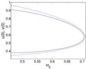
Figure 1: (Color Online) Amplitude of the couplers for the asymmetric solution in the Hamiltonian case of $\gamma=0$ and for $s=\sqrt{63}/32$, $\epsilon=1$ (left panel) and $s=\sqrt{15}/8$, $\epsilon=-1$ (right panel). The dashed lines correspond to the predictions of the RWA theory (see the discussion in the text). It is worth noticing that in the left panel, asymmetric solutions are unstable towards finite time blow up for frequencies smaller than those shown in the figure. On the contrary, in the right panel, solutions are always stable for frequencies higher than those shown in the picture.

V.1 Soft potential

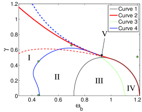
Figure 2: (Color Online) Plane with curves and regions of solutions that share the same properties when $\epsilon=1$ and $s=\sqrt{15}/8$ (see text). In the non-labeled region of the top right, neither S nor A solutions exist. Here Curve 1 corresponds to the linear limit, Curve 2 denotes the $\mathcal{P}\mathcal{T}$ phase transition curve, Curve 3 indicates the destabilization of the A branch, while Curve 4 is associated with the destabilization of the symmetric branch. The detailed description of the different regions enclosed by the curves is offered in the text. Dashed lines correspond to the RWA predictions. Notice that the colors of the dashed lines are inverted with respect to that of the numerical results for a better visualization. I.e., the blue dashed line is the theoretical prediction corresponding to the red solid one, while the red dashed line represents the prediction corresponding to the blue solid one. This inversion pattern is followed also in all figures comparing theory and numerical computations from here on. Dots mark the parameters for which simulations are performed in Fig. 5.

We analyze firstly the soft case ($\epsilon=+1$) in the presence now of the gain/loss term proportional to $\gamma$. Figure 2 shows a $\gamma$-$\omega_{\mathrm{b}}$ full two-parameter plane summarizing the existence properties of the solutions and separating the different regimes thereof.

• Curve 1 corresponds to the linear modes, obtained in section II; The increasing part of the curve fulfills $\omega_{1}=\sqrt{1-\gamma^{2}/2-\sqrt{s^{2}-\gamma^{2}+\gamma^{4}/4}}$ and corresponds to symmetric linear modes at $\gamma=0$; the decreasing part $\omega_{2}=\sqrt{1-\gamma^{2}/2+\sqrt{s^{2}-\gamma^{2}+\gamma^{4}/4}}$ holds for the branch stemming from the anti-symmetric linear modes of $\gamma=0$ [cf. with Eq. (7)]. These two classes of linear modes collide and disappear hand-in-hand at the value of $\gamma$ predicted by Eq. (8). For this soft case, solutions are expected to exist (in analogy with the Schrödinger case) for $\omega_{\mathrm{b}}<\omega_{1}$ for the symmetric branch and for $\omega_{\mathrm{b}}<\omega_{2}$ for the anti-symmetric branch (for a given value of $\gamma$).

• Curve 2 corresponds to the $\mathcal{P}\mathcal{T}$ phase transition, i.e., at the nonlinear level it corresponds to the saddle-center bifurcation leading to the termination of both the A and S branches. Above this curve, there do not exist any periodic orbits and the system dynamics generically leads to indefinite growth. This curve overlaps with Curve 1 for high $\omega_{\mathrm{b}}$.

• Curves 3 and 4 separate stable and unstable solutions of the anti-symmetric and symmetric branches, respectively. In particular, they represent the threshold for the symmetry-breaking bifurcation of the corresponding branches.

The regions limited by the curves above are the following ones:

• Region I: Both solutions S and A are unstable, as they have both crossed the instability inducing curves 3 and 4.

• Region II: Solutions S are stable (as they have not crossed curve 4) whereas A are unstable (as bifurcating from the decreasing part of curve 1, they have crossed the instability threshold of curve 3).

• Region III: Solutions S do not exist (as such solutions only exist to the left of the increasing part of curve 1) and solutions A are unstable (as they have crossed the instability threshold of curve 3).

• Region IV: Solutions S do not exist (for the same reason as in III) and solutions A are stable. I.e., they are stable between their bifurcation point –decreasing part of curve 1– and instability threshold –curve 3–.

• Region V: Stable A and S solutions coexist in this narrow region prior to their termination in the saddle-center bifurcation occurring on Curve 2.

In Fig. 3, some typical examples of mono-parametric continuations of the relevant solutions are given. The top panels illustrate continuations as a function of the gain/loss parameter $\gamma$ for a fixed value of the frequency $\omega_{\mathrm{b}}=0.45$, while the bottom ones illustrate a continuation as a function of $\omega_{\mathrm{b}}$ for a given value of $\gamma=0.4$. The comparison of the numerically obtained symmetric and anti-symmetric solutions with the ones obtained analytically by virtue of the RWA (in reverse colors– see the figure) is also offered. It can be inferred that generally the RWA offers reasonable qualitative match to the numerically exact, up to a prescribed tolerance, solutions, although clearly quantitative comparison is less good, at least for the low (i.e., far from the linear limit) value of $\omega_{\mathrm{b}}$ in the top panels. This deficiency of the method (explained also previously) as one departs far from the linear limit is more clearly illustrated in the $\omega_{\mathrm{b}}$ dependence. Close to the limit, the RWA does an excellent job of capturing both branches, but things become progressively worse as $\omega_{\mathrm{b}}$ decreases. Furthermore, as discussed above the right panels showcase a stability change as occurring for both branches, while the RWA predicts a destabilization solely of the symmetric branch for this soft nonlinearity case.

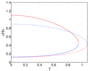
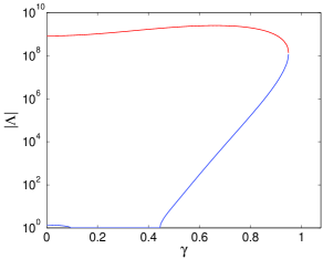
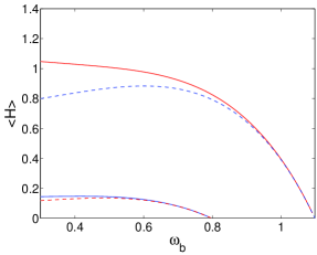
Figure 3: (Color Online) Averaged energy (top left) and modulus of the Floquet multipliers (top right) [only the multipliers with moduli higher than one are shown] as a function of the gain/loss parameter $\gamma$ for $\epsilon=1$, $\omega_{\mathrm{b}}=0.45$, and $s=\sqrt{15}/8$. Notice the logarithmic scale in the $y$-axis of the latter graph. In the left panel, blue (red) solid line corresponds to the S (A) solution, while red (blue), i.e., reversed colors, dashed lines correspond to the S (A) branch RWA predictions. One can observe a reasonable agreement between the numerical energy and its theoretical prediction counterpart, although some discrepancy is clearly visible for this low (i.e., far from the linear limit) value of the frequency. The bottom panel shows similar comparisons but now for the dependence on $\omega_{\mathrm{b}}$ for fixed $\gamma=0.4$. Here it is evident that the agreement is good close to the linear limit of larger values of $\omega_{\mathrm{b}}$ and progressively worsens as one departs from this limit (by lowering the breather frequency).

In the above two-parametric diagram, we have only varied the frequency of the breathers $\omega_{\mathrm{b}}$ and the strength of the gain/loss $\gamma$. To illustrate how the results vary as the final (coupling) parameter of the system varies, we have illustrated the same features as in Figs. 2-3 for roughly half the coupling strength in Fig. 4. We observe that the region of stability of the different solutions (and especially of the symmetric one) has non-trivially changed upon the considered parametric variation. Nevertheless, sufficiently close to the linear limit of emergence of the two solutions, the RWA remains a reasonable description of their existence and stability, as well as of the saddle-center bifurcation leading to their disappearance. On the other hand, as one further deviates from this limit towards lower frequencies, the RWA fails to capture the observed phenomenology by deviating from the critical point for the saddle-center bifurcation, missing the complex boundary of stability of the symmetric branch and missing altogether the destabilization of the anti-symmetric branch.

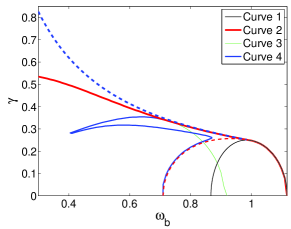
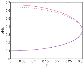
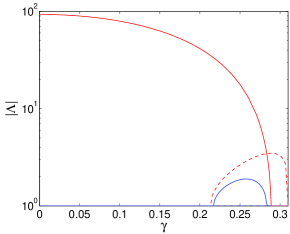
Figure 4: (Color Online) Same as the Fig. 2 (top panel) and as the top panel of Fig. 3 (bottom panels) but for the soft nonlinearity case of lower coupling $s=\sqrt{63}/32$. Again the full numerical results are offered by the solid lines for the two branches (blue for S and red for A), while the dashed lines with reverse colors correspond to the RWA.

Some examples of the evolution of unstable solutions for $s=\sqrt{15}/8$ are shown at Fig. 5. In these cases, the perturbation was induced solely from numerical truncation errors. In most cases, the instabilities lead to finite time blow-up, whereas in some cases a switching between the oscillators is observed i.e., a modulated variant of the time-periodic solution arises as a result of the instability. However, generally speaking, if the perturbation is above a threshold and/or the value of the gain/loss parameter $\gamma$ is sufficiently high and/or the solution frequency sufficiently low, the instability manifestation will typically result in a finite time blow-up. This is strongly related to the escape dynamics considered in escape . On the contrary, we want to highlight that this is different than the “worst case scenario” of the Schrödinger dimer of the RWA. As illustrated in Pelinov , in the latter at worst an exponential (indefinite) growth of the amplitude may arise (but no finite time blow up). Our numerical computations indicate that the switching behavior reported above is only possible provided that the growth rate (i.e. the FE) of the periodic solution is small enough. For S (A) solutions, this can be achieved close to curve 4 (3). This condition is, however, not sufficient, as shown in the top right panel of Fig. 5. We have also analyzed the outcome for solutions with $\gamma>\gamma_{SC}$, taking as initial condition a solution for $\gamma<\gamma_{SC}$; in that case, we have observed that, although the generic scenario corresponds to a blow-up, isolated cases of modulated dynamics may arise when such a profile is used as initial condition for the simulation.

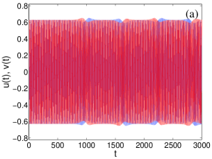
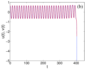
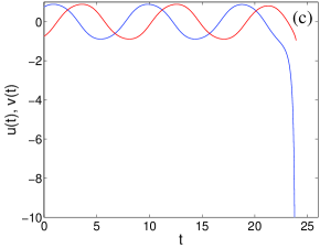
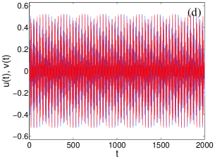
Figure 5: (Color Online) Evolution of unstable solutions for the soft potential; the instability is driven only by the numerical truncation errors. (Top left panel) S solution with $\omega_{\mathrm{b}}=0.45$ and $\gamma=0.01$. (Top right panel) S solution with $\omega_{\mathrm{b}}=0.45$ and $\gamma=0.45$. (Bottom left panel) A solution with $\omega_{\mathrm{b}}=0.70$ and $\gamma=0.66$. (Bottom right panel) The A solution at $\gamma=0.16$ and $\omega_{\mathrm{b}}=1.2$ is taken at initial condition for $\gamma=0.51$; notice that for this value of $\omega_{\mathrm{b}}$, the saddle-center bifurcation takes place at $\gamma_{SC}=0.168$.

V.2 Hard potential

We now briefly complement these results with ones of the far more accurately approximated (by the RWA) hard potential case. This disparity in the much higher level of adequacy of the theoretical approximation here is clearly induced by the absence of finite-time collapse in the latter model in consonance (in this case) with its RWA analog.

In this case, the branches exist to the right of the linear curve (for a given $\gamma$), as is expected in the case of a hard/defocusing nonlinearity. Curve 1 illustrates the linear limit; once again its growing part ($\omega_{1}$) is associated with the symmetric solutions, while its decreasing part ($\omega_{2}$) with the ant-symmetric solutions, with their collision point representing the linear $\mathcal{P}\mathcal{T}$ transition point. In fact, from that point, emanates curve 2 which is the nonlinear $\mathcal{P}\mathcal{T}$ phase transition curve i.e., the locus of points where the S and A solutions collide and disappear for the nonlinear problem. Notice the very good comparison of this curve with the theoretical prediction of the RWA for $\gamma_{SC}$. Curve 3, on the other hand, denotes the point of destabilization of the A branch, which is in fact expected also from the RWA, whose prediction is once again (red dashed line) in remarkable agreement with the full numerical result. The final curve in the graph, i.e., the green solid line of Curve 4 denotes a narrow parametric window beyond which (or more appropriately between which and Curve 2) even the S branch of time-periodic solutions is destabilized. This, as indicated previously, is a feature that is not captured by the RWA but is unique to the oscillator system (as is correspondingly the destabilization of the A branch in the soft potential case). We now discuss the existence and stability of the branches in each of the regions between the different curves.

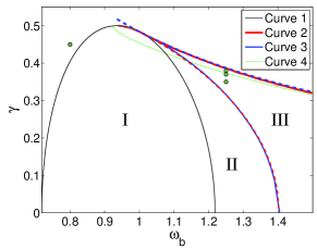
Figure 6: (Color Online) Same as Fig. 2 but in the hard potential case, i.e. when $\epsilon=-1$. The only change with respect to that figure consists of an interchange of the color / thickness between Curves 3 and 4. Dots mark the parameters for which simulations are performed in Fig. 8.

• Region I: Only S solutions exist (i.e., to the right of the increasing part of Curve 1, but to the left of its decreasing part). They bifurcate from the linear modes when $\omega_{\mathrm{b}}\geq\omega_{1}$. The S modes are stable in this regime.

• Region II: Solutions S and A exist and are both stable. The A solutions have now bifurcated for $\omega_{\mathrm{b}}>\omega_{2}$.

• Region III: Solutions S are stable whereas solutions A are unstable. Here, the symmetry breaking bifurcation destabilizing the anti-symmetric solutions has taken place in close accord with what is expected from the RWA.

• Finally, there is a Region (IV) between the (green) thin solid line of Curve 4 and the thick solid (red) line of Curve 2 denoting the narrow parametric regime where the S branch is unstable.

Similarly to Fig. 3 in Fig. 7, we offer monoparametric continuation examples (i.e., vertical or horizontal cuts along the two parameter diagram of Fig. 6. Both along the vertical cuts of the $\gamma$ dependence for $\omega_{\mathrm{b}}=1.25$ in the top panels, as well as along the horizontal cuts for $\gamma=0.3$ in the bottom panels, it can be seen that the dashed lines of the RWA do a very reasonable (even quantitatively) job of capturing the features of the full periodic solutions. As discussed above, the only example where a trait is missed by the RWA is the narrow instability interval of the symmetric branch of the blue solid line in the top right panel of Fig. 7.

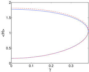
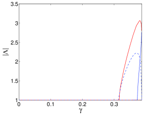
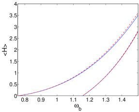
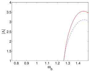
Figure 7: (Color Online) Similar to Fig. 3 but for $\omega_{\mathrm{b}}=1.25$ and $\epsilon=-1$ in the top panels and for $\gamma=0.3$ and $\epsilon=-1$ in the bottom panels. Both the existence (left) and stability (right) diagrams of S (blue solid) and A (red solid) branches and their rotating wave approximations (the latter with reverse colors and dashed lines) are shown.

Two examples of the evolution of unstable solutions are shown at Fig. 8. In these cases, the perturbation came only from numerical truncation errors. The most typical dynamical evolution consists of a continuous gain of the oscillator $u(t)$ which is accompanied by a vanishing of the oscillations of $v(t)$. However, notice that in this case and in agreement with the expectations from the RWA and Schrödinger $\mathcal{P}\mathcal{T}$-symmetric dimer, the indefinite growth does not arise at a finite time (i.e., finite time blowup) but instead emerges as an apparent (modulated) exponential growth on the one node, associated with decay in the second one. However, we should highlight an additional possibility which can arise in the form of a quasi-periodic orbit, if the perturbation is small enough. This dynamical behavior can turn into the gain / vanishing one, as the size of the perturbation is increased. Let us mention that although A solutions are mostly prone to indefinite growth, there are some cases where instability could manifest itself as switching; at a given value of $\omega_{\mathrm{b}}$, our simulations indicate that switching occurs at a range of intermediate values of $\gamma$. For instance, for $\omega_{\mathrm{b}}=1.25$, the A solution is unstable in the range $\gamma\in[0.316,0.386]$ and switching (i.e., modulation of the periodic orbit) takes place for $0.35\lesssim\gamma\lesssim 0.36$. S solutions offer a similar trend.

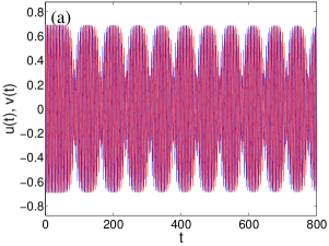
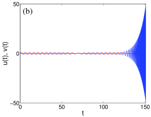
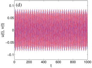
Figure 8: (Color Online) Evolution of unstable solutions for the hard potential; the instability is driven only by the numerical truncation errors. (Top left panel) A solution with $\omega_{\mathrm{b}}=1.25$ and $\gamma=0.35$. (Top right panel) A solution with $\omega_{\mathrm{b}}=1.25$ and $\gamma=0.37$. (Bottom left panel) S solution with $\omega_{\mathrm{b}}=1.25$ and $\gamma=0.38$. (Bottom right panel) The S solution at $\gamma=0.4$ and $\omega_{\mathrm{b}}=0.8$ is taken at initial condition for $\gamma=0.45$; notice that for this value of $\gamma$, the saddle-center bifurcation takes place at $\gamma_{SC}=0.404$.

VI Conclusions and Future Challenges

In the present work, we have considered a prototypical example of a $\mathcal{P}\mathcal{T}$-symmetric dimer in the context of coupled nonlinear oscillators. We explored how the behavior of the Hamiltonian limit of the system is modified in the presence of the gain/loss parameter $\gamma$ which plays a significant role in the dynamics. We were able to quantify the existence, stability and nonlinear dynamics of the model numerically by means of a Newton solver identifying periodic orbits, coupled to a Floquet exponent computation, as well as a time-stepper of the system’s evolution. We also provided a useful theoretical approximation to the relevant features by means of a Schrödinger dimer via the rotating wave approximation but also delineated the limitations of such an approach. Through the combination of these tools, we observed how symmetric and anti-symmetric periodic orbits bifurcate from a quantifiable linear limit, how they become unstable through symmetry-breaking bifurcations and finally how they terminate in a nonlinear analog of the $\mathcal{P}\mathcal{T}$ transition. While most of these features could be theoretically understood by means of our (linear and nonlinear RWA) analysis, we also revealed a set of effects particular to the oscillator system, such as the possibility for escape and finite time collapse in the case of soft nonlinearity, as well as the potential for destabilization of both branches (rather than just the single one suggested by RWA). We also explained the regime where the RWA was expected to be most efficient (i.e., for parameters proximal to the bifurcation from the linear limit) and where more significant deviations should be expected, most notably e.g. for much smaller frequencies $\omega_{\mathrm{b}}$ in the soft potential case.

This work, we believe, paves the way for a number of future considerations in the context of oscillator problems with $\mathcal{P}\mathcal{T}$ symmetry. While in the Schrödinger context, numerous studies have addressed the large/infinite number of nodes limit Pelin1 ; Sukh ; zheng , this is far less so the case in the context of oscillators where this analysis is really at a nascent stage. In such lattice contexts, it would be of particular interest to consider genuine breather type solutions in the form of exponentially localized in space and periodic in time orbits. Once such structures are identified systematically in the context of 1d settings, it would also be natural to extend consideration to higher dimensional plaquettes Guenter and lattices, where more complex patterns (including discrete vortices among others aubry ) are known to be possible. Such studies are currently in progress and will be reported in future publications.

References

- (1) C. M. Bender and S. Boettcher, Phys. Rev. Lett. 80, 5243 (1998).
- (2) C. M. Bender, Rep. Prog. Phys. 70, 947 (2007).
- (3) C. M. Bender, S. Boettcher, and P. N. Meisinger, J. Math. Phys. 40, 2201 (1999).
- (4) Z. H. Musslimani, K. G. Makris, R. El-Ganainy, and D. N. Christodoulides, Phys. Rev. Lett. 100, 030402 (2008); K. G. Makris, R. El-Ganainy, D. N. Christodoulides, and Z. H. Musslimani, Phys. Rev. Lett. 100, 103904 (2008).
- (5) A. Ruschhaupt, F. Delgado, and J.G. Muga, J. Phys. A: Math. Gen. 38, L171–L176 (2005).
- (6) A. Guo, G. J. Salamo, D. Duchesne, R. Morandotti, M. Volatier-Ravat, V. Aimez, G. A. Siviloglou, and D. N. Christodoulides, Phys. Rev. Lett. 103, 093902 (2009).
- (7) C.E. Rüter, K.G. Makris, R. El-Ganainy, D.N. Christodoulides, M.Segev, and D. Kip, Nature Physics 6, 192 (2010).
- (8) S.V. Dmitriev, A.A. Sukhorukov, and Yu.S. Kivshar, Opt. Lett. 35, 2976 (2010).
- (9) K. Li and P.G. Kevrekidis, Phys. Rev. E 83, 066608 (2011).
- (10) K. Li, P.G. Kevrekidis, B.A. Malomed, and U. Günther, J. Phys. A Math. Theor. 45, 444021 (2012).
- (11) H. Ramezani, T. Kottos, R. El-Ganainy, and D.N. Christodoulides, Phys. Rev. A 82, 043803 (2010).
- (12) S.V. Suchkov, B.A. Malomed, S.V. Dmitriev, and Yu.S. Kivshar, Phys. Rev. E 84, 046609 (2011).
- (13) A.A. Sukhorukov, Z. Xu, and Yu.S. Kivshar, Phys. Rev. A 82, 043818 (2010).
- (14) D.A. Zezyulin and V.V. Konotop, Phys. Rev. Lett. 108, 213906 (2012).
- (15) V.V. Konotop, D.E. Pelinovsky, and D.A. Zezyulin, EPL 100, 56006 (2012).
- (16) A.A. Sukhorukov, S.V. Dmitriev, S.V. Suchkov, and Yu.S. Kivshar, Opt. Lett. 37, 2148 (2012).
- (17) M.C. Zheng, D.N. Christodoulides, R. Fleischmann, and T. Kottos, Phys. Rev. A 82, 010103(R) (2010).
- (18) J. Schindler, A. Li, M.C. Zheng, F.M. Ellis, and T. Kottos, Phys. Rev. A 84, 040101(R) (2011).
- (19) J. Schindler, Z. Lin, H. Ramezani, F.M. Ellis, and T. Kottos, J. Phys. A 45, 444029 (2012).
- (20) N. Lazarides, G.P. Tsironis, Phys. Rev. Lett. 110, 053901 (2013).
- (21) D.K. Campbell, J.F. Schonfeld, and C.A. Wingate, Phys. D. 9, 1 (1983).
- (22) T.I. Belova and A.E. Kudryavtsev, Phys. Uspekhi 40, 359 (1997).
- (23) P.G. Kevrekidis, D.E. Pelinovsky, and D.Y. Tyugin, arXiv:1303.3298, SIAM J. Appl. Dyn. Sys. (in press, 2013); also: P.G. Kevrekidis, D.E. Pelinovsky, and D.Y. Tyugin, arXiv:1307.2973.
- (24) J. Pickton, H. Susanto, arXiv:1307.2788.
- (25) V. Achilleos, A. Álvarez, J. Cuevas, D.J. Frantzeskakis, N.I. Karachalios, P.G. Kevrekidis, and B. Sánchez-Rey, Physica D 244, 1 (2013).
- (26) J. Cuevas, J.F.R. Archilla, and F.R. Romero, J. Phys. A: Math. Theor. 44, 035102 (2011).
- (27) J.F.R. Archilla, R.S. MacKay, and J.L. Marín Physica D 134, 406 (1999).
- (28) J.L. Marín Intrinsic Localized Modes in nonlinear lattices. PhD Thesis, University of Zaragoza (1999)
- (29) J. Cuevas Localization and energy transfer in anharmonic inhomogeneus lattices PhD Thesis, University of Sevilla (2003)
- (30) A.S. Rodrigues, K. Li, V. Achilleos, P.G. Kevrekidis, D.J. Frantzeskakis, and C.M. Bender, Romanian Rep. Phys. 65, 5 (2013).
- (31) Yu.S. Kivshar and M. Peyrard. Phys. Rev. A 46, 3198 (1992).
- (32) K.W. Sandusky, J.B. Page, and K.E. Schmidt. Phys. Rev. B 46, 6161 (1992).
- (33) A.M. Morgante, M. Johansson, G. Kopidakis, and S. Aubry. Physica D 162, 53 (2002).
- (34) T. Cretegny and S. Aubry Phys. Rev. B 55, R11929 (1997).