Quantum Optical Realization of Classical Linear Stochastic Systems

Abstract

The purpose of this paper is to show how a class of classical linear stochastic systems can be physically implemented using quantum optical components. Quantum optical systems typically have much higher bandwidth than electronic devices, meaning faster response and processing times, and hence has the potential for providing better performance than classical systems. A procedure is provided for constructing the quantum optical realization. The paper also describes the use of the quantum optical realization in a measurement feedback loop. Some examples are given to illustrate the application of the main results.

^,∗, , ,

1 Introduction and Motivation

With the birth and development of quantum technologies, quantum control systems constructed using quantum optical devices play a more and more important role in control engineering, [Wiseman $\&$ Milburn (1993)], [Wiseman $\&$ Milburn (1994)], and [Wiseman $\&$ Milburn (2009)]. Linear systems are of basic importance to control engineering, and also arise in the modeling and control of quantum systems; see [Gardiner $\&$ Zoller (2004)] and [Wiseman $\&$ Milburn (2009)]. A classical linear system described by the state space representation can be realized using electrical and electronic components by linear electrical network synthesis theory, see [Anderson $\&$ Vongpanitlerd (1973)]. For example, consider a classical system given by

$$d\xi(t)= -\xi(t)dt+dv_{1}(t)$$

$$dy(t)= \xi(t)dt+dv_{2}(t)$$ (1)

where $\xi(t)$ is the state, $v_{1}(t)$ and $v_{2}(t)$ are inputs, and $y(t)$ is the output. Implementation of the system (1) at the hardware level is shown in Figure 1. Analogously to the electrical network synthesis theory of how to synthesize linear analog circuits from basic electrical components, [Nurdin et al.(2009)] have proposed a quantum network synthesis theory (briefly introduced in Subsection 2.4 of this paper), which details how to realize a quantum system described by state space representations using quantum optical devices.

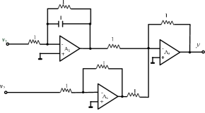
Figure 1: Classical hardware implementation of the system (1).

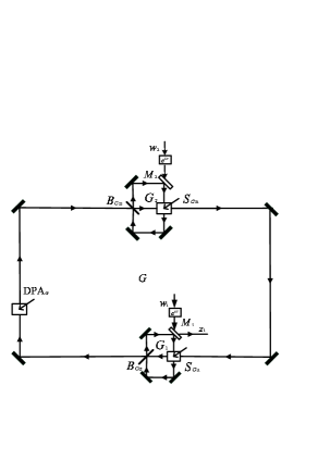
Figure 2: Quantum hardware realization of the system (1).

The purpose of this paper is to address this issue of quantum physical realization for a class of classical linear systems. For example, the quantum physical realization of the system (1) is shown in Figure 2 (see Example 1 in Section 3 for more details). The essential quantum optical components used in Figure 2 include optical cavities, degenerate parametric amplifiers (DPA), phase shifters, beam splitters, and squeezers, etc; interested readers may refer to [Bachor $\&$ Ralph (2004)], [Nurdin et al.(2009)] for a more detailed introduction to these optical devices. The problem of quantum physical realization can be solved by embedding the classical system into a larger linear quantum system, Theorem 1. In this way, the classical system is represented as an invariant commutative subsystem of the larger quantum system.

While the results of this paper may be useful for a variety of problems outside the scope of measurement feedback control, the principle motivation for realizing classical systems in quantum hardware is that one is better able to match the timescales and hardware of a classical controller to the system being controlled. Classical hardware is typically much slower than the quantum systems intended to be controlled, and complex interface hardware may be required. Compared with classical systems typically implemented using standard analog or digital electronics, quantum mechanical systems may provide a bandwidth much higher than that of conventional electronics and thus increase processing times. For instance, quantum optical systems can have frequencies up to $10^{14}$ Hz or higher. Furthermore, it is becoming feasible to implement quantum networks in semiconductor materials, for example, photonic crystals are periodic optical nanostructures that are designed to affect the motion of photons in a similar way that periodicity of a semiconductor crystal affects the motion of electrons, and it may be desirable to implement control networks on the same chip (rather than interfacing to a separate system); see [Beausoleil et al.(2007)].

This paper is organized as follows. Section 2 introduces some notations of classical and quantum random variables and then gives a brief overview of classical linear systems, quantum linear stochastic systems as well as quantum network synthesis theory. Section 3 presents the main results of this paper, which are illustrated with an example. Section 4 presents a potential application of the main results of Section 3 to measurement feedback control of quantum systems. Finally, Section 5 gives the conclusion of this paper.

Notation. The notations used in this paper are as follows: $i=\sqrt{-1}$; the commutator is defined by $[A,B]=AB-BA$. If $X=[x_{jk}]$ is a matrix of linear operators or complex numbers, then $X^{\#}=[x^{*}_{jk}]$ denotes the operation of taking the adjoint of each element of $X$, and $X^{{\dagger}}=[x^{*}_{jk}]^{T}$ . We also define $\Re(X)=(X+X^{\#})/2$ and $\Im(X)=(X-X^{\#})/2i$, and $\mathrm{diag}_{n}(M)$ denotes a block diagonal matrix with a square matrix $M$ appearing $n$ times on the diagonal block. The symbol $I_{n}$ denotes the $n\times n$ identity matrix, and we write

$$J_{n}=\left[\begin{array}[]{cc}0&I_{n}\\ -I_{n}&0\end{array}\right].$$ (4)

2 Preliminaries

2.1 Classical and quantum random variables

Recall that a random variable $X$ is Gaussian if its probability distribution $\mathbf{P}$ is Gaussian, i.e.

$$\mathbf{P}(a<X<b)=\int_{a}^{b}p_{X}(x)dx,$$ (5)

where $p_{X}(x)=\frac{1}{\sigma\sqrt{2\pi}}\mathrm{exp}(-\frac{(x-\mu)^{2}}{2\sigma^{2}})$. Here, $\mu=\mathbf{E}[X]$ is the mean, and $\sigma^{2}=\mathbf{E}[(X-\mu)^{2}]$ is the variance.

In quantum mechanics, observables are mathematical representations of physical quantities that can (in principle) be measured, and state vectors $\psi$ summarize the status of physical systems and permit the calculation of expected values of observables. State vectors may be described mathematically as elements of a Hilbert space $\mathfrak{H}=L^{2}(\mathbf{R})$ of square integrable complex-valued functions on the real line, while observables are self-adjoint operators $A$ on $\mathfrak{H}$. The expected value of an observable $A$ when in pure state $\psi$ is given by the inner product $\langle\psi,A\psi\rangle=\int_{-\infty}^{\infty}\psi(q)^{*}A\psi(q)dq$. Observables are quantum random variables.

A basic example is the quantum harmonic oscillator, a model for a quantum particle in a potential well; see [Merzbacher (1998), Chapter 14]. The position and momentum of the particle are represented by observables $Q$ and $P$ (also called position quadrature and momentum quadrature), respectively, defined by

$$(Q\psi)(q)=q\psi(q),\ \ \ (P\psi)(q)=-i\frac{d}{dq}\psi(q)$$ (6)

for $\psi\in\mathfrak{H}=L^{2}(\mathbf{R})$. Here, $q\in\mathbf{R}$ represents position values. The position and momentum operators do not commute, and in fact satisfy the commutation relation $[Q,P]=i$. In quantum mechanics, such non-commuting observables are referred to as being incompatible. The state vector

$$\psi(q)=(2\pi)^{-\frac{1}{4}}\sigma^{-\frac{1}{2}}\mathrm{exp}(-\frac{(q-\mu)^{2}}{4\sigma^{2}})$$ (7)

is an instance of what is known as a Gaussian state. For this particular Gaussian state, the means of $P$ and $Q$ are given by $\int_{-\infty}^{\infty}\psi(q)^{*}Q\psi(q)dq=\mu$, and $\int_{-\infty}^{\infty}\psi(q)^{*}P\psi(q)dq=0$, and similarly the variances are $\sigma^{2}$ and $\frac{\hbar^{2}}{4\sigma^{2}}$, respectively.

If we are given a classical vector-valued random variable $\widetilde{X}=[X_{1}\quad X_{2}\quad\cdots\quad X_{n}]^{T}$, we may realize (or represent) it using a quantum vector-valued random variable $\check{X}_{Q}$ with associated state $\psi$ in a suitable Hilbert space in the sense that the distribution of $\widetilde{X}$ is the same as the distribution of $\check{X}_{Q}$ with respect to the state $\psi$. For instance, if the variable $\widetilde{X}$ have a multivariate Gaussian distribution with its probability density function given by

$$f(\tilde{x})=(2\pi)^{-\frac{n}{2}}|\Sigma|^{-\frac{1}{2}}\mathrm{exp}\left(-\frac{1}{2}(\tilde{x}-\tilde{\mu})^{T}\Sigma^{-1}(\tilde{x}-\tilde{\mu})\right)$$ (8)

with mean $\tilde{\mu}\in\mathbb{R}^{n}$ and covariance matrix $\Sigma\in\mathbb{R}^{n\times n}$, we may realize this classical random variable $\widetilde{X}$ using an open harmonic oscillator. Indeed, we can take the realization to be the position quadrature $\check{X}_{Q}=[Q_{1}^{T}\quad Q_{2}^{T}\quad\cdots\quad Q_{n}^{T}]^{T}$ (for example), with the state $\psi$ selected so that $(\tilde{\mu},\Sigma^{2})=(\tilde{\mu}_{Q},\Sigma_{Q}^{2})$. So statistically $\widetilde{X}\equiv\check{X}_{Q}$. The quantum vector $\check{X}=[\check{X}_{Q}^{T}\quad\check{X}_{P}^{T}]^{T}$ is called an augmentation of $\widetilde{X}$, where $\check{X}_{P}=[P_{1}^{T}\quad P_{2}^{T}\quad\cdots\quad P_{n}^{T}]^{T}$ is the momentum quadrature. The quantum realization of the classical random variable may be expressed as $\widetilde{X}\equiv\left[\begin{array}[]{cc}I_{n}&0_{n\times n}\end{array}\right]\left[\begin{array}[]{c}\check{X}_{Q}\\ \check{X}_{P}\end{array}\right].$

2.2 Classical linear systems

Consider a class of classical linear systems of the form,

$$d\xi(t)= A\xi(t)dt+Bdv_{1}(t),$$

$$dy(t)= C\xi(t)dt+Ddv_{2}(t),$$ (9)

where $A\in\mathbb{R}^{n\times n}$, $B\in\mathbb{R}^{n\times n_{v_{1}}}$, $C\in\mathbb{R}^{n_{y}\times n}$ and $D\in\mathbb{R}^{n_{y}\times n_{v_{2}}}$ are real constant matrices, $v_{1}(t)$ and $v_{2}(t)$ are input signals and independent. The initial condition $\xi(0)=\xi_{0}$ is Gaussian, while $y(0)=0$. The transfer function $\Xi_{C}(s)$ from the noise input channel $v$ to the output channel $y$ for the classical system (9) is denoted by

$$\Xi_{C}(s)= \left[\begin{tabular}[]{l|ll}$A$&$\left[\begin{array}[]{cc}B,&0_{n\times n_{v_{2}}}\\ \end{array}\right]$\\ \hline\cr\vspace{0em} $C$&$\left[\begin{array}[]{cc}0_{n_{v_{2}}\times n_{v_{2}}},&D\\ \end{array}\right]$\\ \end{tabular}\right](s)=\left[\begin{array}[]{cc}C\left(sI_{n}-A\right)^{-1}B,&D\\ \end{array}\right]$$ (15)

2.3 Quantum linear stochastic systems

Consider a quantum linear stochastic system of the form (see e.g. [Gardiner $\&$ Zoller (2004)], [Wiseman $\&$ Milburn (2009)], [Nurdin et al.(2009)])

$$dx(t)= \widetilde{A}x(t)dt+\widetilde{B}dw(t),$$

$$dz(t)= \widetilde{C}x(t)dt+\widetilde{D}dw(t),$$ (16)

where $\widetilde{A}\in\mathbb{R}^{2n\times 2n}$, $\widetilde{B}\in\mathbb{R}^{2n\times n_{w}}$, $\widetilde{C}\in\mathbb{R}^{n_{z}\times 2n}$ and $\widetilde{D}\in\mathbb{R}^{n_{z}\times n_{w}}$ are real constant matrices. We assume that $n_{w}$ and $n_{z}$ are even, with $n_{z}\leq n_{w}$ (see [James et al.(2008), Section II] for details). We refer to $n$ as the degrees of freedom of systems of the form (2.3). Equation (2.3) is a quantum stochastic differential equation (QSDE) [Parthasarathy (1992)] and [Gardiner $\&$ Zoller (2004)]. In equation (2.3), $x(t)$ is a vector of self-adjoint possibly non-commuting operators, with the initial value $x(0)=x_{0}$ satisfying the commutation relations

$$x_{0j}x_{0k}-x_{0k}x_{0j}=2i\widetilde{\Theta}_{jk},$$ (17)

where $\widetilde{\Theta}=[\widetilde{\Theta}_{jk}]_{j,k=1,2,\ldots,2n}$ is a skew-symmetric real matrix. The matrix $\widetilde{\Theta}$ is said to be canonical if it is the form $\widetilde{\Theta}=J_{n}$. The components of the vector $w(t)$ are quantum stochastic processes with the following non-zero Ito products:

$$dw_{j}(t)dw_{k}(t)=F_{jk}dt,$$ (18)

where $F$ is a non-negative definite Hermitian matrix. The matrix $F$ is said to be canonical if it is the form $F=I_{n_{w}}+iJ_{\frac{n_{w}}{2}}$. In this paper we will take $\widetilde{\Theta}$ and $F$ to be canonical. The transfer function for the quantum linear stochastic system (2.3) is given by

$$\Xi_{Q}(s)=\left[\begin{tabular}[]{l|ll}$\widetilde{A}$&$\widetilde{B}$\\ \hline\cr\vspace{-1em}\\ $\widetilde{C}$&$\widetilde{D}$\\ \end{tabular}\right](s)=\widetilde{C}\left(sI_{2n}-\widetilde{A}\right)^{-1}\widetilde{B}+\widetilde{D}.$$ (22)

Here we mention that while the equations (2.3) look formally like the classical equations (9), they are not classical equations, and in fact give the Heisenberg dynamics of a system of coupled open quantum harmonic oscillators. The variables $x(t)$, $w(t)$ and $z(t)$ are in fact vectors of quantum observables (self-adjoint non-commuting operators, or quantum stochastic processes).

The quantum system (2.3) is (canonically) physically realizable (cf.[Wang et al.(2012)]), if and only if the matrices $\widetilde{A}$, $\widetilde{B}$, $\widetilde{C}$ and $\widetilde{D}$ satisfy the following conditions:

$$\widetilde{A}J_{n}+J_{n}\widetilde{A}^{T}+\widetilde{B}J_{\frac{n_{w}}{2}}\widetilde{B}^{T}=0,$$ (23)

$$\widetilde{B}J_{\frac{n_{w}}{2}}\widetilde{D}^{T}=-J_{n}\widetilde{C}^{T},$$ (24)

$$\widetilde{D}J_{\frac{n_{w}}{2}}\widetilde{D}^{T}=J_{\frac{n_{z}}{2}}.$$ (25)

where $n_{w}\geq n_{z}$. In fact, under these conditions the quantum linear stochastic system (2.3) corresponds to an open quantum harmonic oscillator [James et al.(2008), Theorem 3.4] consisting of $n$ oscillators (satisfying canonical commutation relations) coupled to $n_{w}/2$ fields (with canonical Ito products and commutation relations). In particular, in the canonical case, $x_{0}=(q_{1},q_{2},\ldots,q_{n},p_{1},p_{2},\ldots,p_{n})^{T}$, where $q_{j}$ and $p_{j}$ are the position and momentum operators of the oscillator $j$ (which constitutes the $j$th of degree of freedom of the system) that satisfy the commutation relations $[q_{j},p_{k}]=2i\delta_{jk}$, $[q_{j},q_{k}]=[p_{j},p_{k}]=0$ in accordance with (17). Hence by the results of [Nurdin et al.(2009)] the system can be implemented using standard quantum optics components. It is also possible to consider other quantum physical implementations.

2.4 Quantum network synthesis theory

We briefly review some definitions and results from [Nurdin et al.(2009)]; see also [Nurdin (2010a)] and [Nurdin (2010b)]. The quantum linear stochastic system (2.3) can be reparametrized in terms of three parameters $S,L,H$ called the scattering, coupling and Hamiltonian operators, respectively. Here $S$ is a complex unitary $\frac{n_{w}}{2}\times\frac{n_{w}}{2}$ matrix $S^{{\dagger}}S=SS^{{\dagger}}=I$, $L=\Lambda x_{0}$ with $\Lambda\in\mathbb{C}^{\frac{n_{w}}{2}\times 2n}$, and $H=\frac{1}{2}x_{0}^{T}Rx_{0}$ with $R=R^{T}\in\mathbb{R}^{2n\times 2n}$. Recall that there is a one-to-one correspondence between the matrices $\tilde{A},\tilde{B},\tilde{C},\tilde{D}$ in (2.3) and the triplet $S,L,H$ or equivalently the triplet $S,\Lambda,R$; see [James et al.(2008)] and [Nurdin et al.(2009)]. Thus, we can represent a quantum linear stochastic system $G$ given by (2.3) with the shorthand notation $G=(S,L,H)$ or $G=(S,\Lambda,R)$ [Gough $\&$ James (2009a)]. Given two quantum linear stochastic systems $G_{1}=(S_{1},L_{1},H_{1})$ and $G_{2}=(S_{2},L_{2},H_{2})$ with the same number of field channels, the operation of cascading of $G_{1}$ and $G_{2}$ is represented by the series product $G_{2}\triangleleft G_{1}$ defined by

$$G_{2}\triangleleft G_{1}=\biggl{(}S_{2}S_{1},L_{2}+S_{2}L_{1},H_{1}+H_{2}\\ +\frac{1}{2i}(L_{2}^{\dagger}S_{2}L_{1}-L_{1}^{\dagger}S_{2}^{\dagger}L_{2})\biggl{)}$$

According to [Nurdin et al.(2009), Theorem 5.1] a linear quantum stochastic system with $n$ degrees of freedom can be decomposed into an unidirectional connection of $n$ one degree of freedom harmonic oscillators with a direct coupling between two adjacent one degree of freedom quantum harmonic oscillators. Thus an arbitrary quantum linear stochastic system can in principle be synthesized if:

1) Arbitrary one degree of freedom systems of the form (2.3) with $n_{w}$ input fields and $n_{w}$ output fields can be synthesized.

2) The bidirectional coupling $H^{d}=\sum^{n-1}_{j=1}\sum^{n}_{k=j+1}x_{k}^{T}\times\\ \left(R_{jk}^{T}-\frac{1}{2i}(\Lambda_{k}^{\dagger}\Lambda_{j}-\Lambda_{k}^{T}\Lambda_{j}^{\#})\right)x_{j}$ can be synthesized, where $\Lambda_{j}$ denotes the $j$th row of the complex coupling matrix $\Lambda$ . The Hamiltonian matrix $R$ is given by $R=\frac{1}{4}P_{2n}^{T}(-J_{n}\widetilde{A}+\widetilde{A}^{T}J_{n})P_{2n}$ and the coupling matrix $\Lambda$ is given by $\Lambda=-\frac{i}{2}\left[\begin{array}[]{cc}0_{n_{w}\times n_{w}}&I_{n_{w}}\\ \end{array}\right]P_{2n_{w}}\mathrm{diag}_{n_{w}}(M)P_{2n_{w}}^{T}\widetilde{B}^{T}J_{n}P_{2n}$ where $M=\left[\begin{array}[]{cc}1&-i\\ 1&i\\ \end{array}\right]$, $P_{2n}$ denotes a permutation matrix acting on a column vector $f=[f_{1}\quad f_{2}\quad...\quad f_{2n}]^{T}$ as $P_{2n}f$=$[f_{1}\quad f_{1+n}\quad f_{2}\quad f_{2+n}\quad...\quad f_{n}\quad f_{2n}]^{T}$.

The work [Nurdin et al.(2009)] then shows how one degree of freedom systems and the coupling $H^{d}$ can be approximately implemented using certain linear and nonlinear quantum optical components. Thus in principle any system of the form (2.3) can be constructed using these components. In Section 3 we will use the construction proposed in [Nurdin et al.(2009)] to realize systems of the form (2.3) without further comment. The details of the construction and the individual components involved can be found in [Nurdin et al.(2009)] and the references therein.

3 Quantum Physical Realization

In this section we present our results concerning the quantum physical realization of classical linear systems and then provide an example to illustrate the results. As is well known, for a linear system, its state space representation can be associated to a unique transfer function representation. Then, we will show how the transfer function matrix $\Xi_{C}(s)$ can be realized (in a sense to be defined more precisely below) using linear quantum components. In general, the dimension of vectors in (2.3) is greater than the vector dimension in (9), and so to obtain a quantum realization of the classical system (9) using the quantum system (2.3) we require that the transfer functions be related by

$$\Xi_{C}(s)=M_{o}\Xi_{Q}(s)M_{i},$$ (26)

as illustrated in Figure 3. Here, the matrix $M_{i}$ and $M_{o}$ correspond to operation of selecting elements of the input vector $w(t)$ and the output vector $z(t)$ of the quantum realization that correspond to quantum representation of $v(t)$ and $y(t)$, respectively (as discussed in Section 2). In Figure 3, the unlabeled box on the left indicates that $v(t)$ is represented as some subvector of $w(t)$ (e.g. modulation), whereas the unlabeled box on the right indicates that $y(t)$ corresponds to some subvector of $z(t)$ (quadrature measurement).

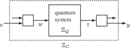
Figure 3: Quantum realization of classical system $\Xi_{C}:v\mapsto y$.

Definition 1.

The classical linear stochastic system (9) is said to be canonically realized by the quantum linear stochastic system (2.3) provided:

1. The dimension of the quantum vectors $x(t)$, $w(t)$ and $z(t)$ are twice the lengths of the corresponding classical vectors $x(t)$, $v(t)=[v_{1}(t)^{T}\quad v_{2}(t)^{T}]^{T}$ and $y(t)$, where $x(t)$=$[\xi(t)^{T}\quad\theta(t)^{T}]^{T}$ with $\xi(t)=[q_{1}(t)\quad q_{2}(t)\quad\cdots\quad q_{n}(t)]^{T}$ and $\theta(t)=[p_{1}(t)\quad p_{2}(t)\\ \quad\cdots\quad p_{n}(t)]^{T}$, $w(t)=[v_{1}(t)^{T}\quad v_{2}(t)^{T}\quad u_{1}(t)^{T}\quad u_{2}(t)^{T}]^{T}$ and $z(t)=[y(t)^{T}\quad y^{\prime}(t)^{T}]^{T}$.

2. The classical $\Xi_{C}(s)$ and quantum $\Xi_{Q}(s)$ transfer functions are related by equation (26) for the choice

   $$M_{o}=\left[\begin{array}[]{cc}I_{n_{y}}&0_{n_{y}\times n_{y}}\\ \end{array}\right],\quad M_{i}=\left[\begin{array}[]{cc}I_{n_{v}}&0_{n_{v}\times n_{v}}\\ \end{array}\right]^{T}.$$

3. The quantum linear stochastic system (2.3) is canonically physically realizable (as described in Section 2.3) with the system matrices $\tilde{A},\tilde{B},\tilde{C}$ and $\widetilde{D}$ having the special structure:

   $$\!\!\!\!\!\!\!\!\!\!\widetilde{A}=\left[\begin{array}[]{cc}A_{0}&0_{n\times n}\\ A_{1}&A_{2}\end{array}\right]\!\!,\widetilde{B}=\left[\begin{array}[]{cccc}B_{0}&0_{n\times n_{v_{2}}}&0_{n\times n_{v_{1}}}&0_{n\times n_{v_{2}}}\\ B_{1}&B_{2}&B_{3}&B_{4}\end{array}\right],$$ (31)

   $$\!\!\!\!\!\!\!\!\!\!\widetilde{C}=\left[\begin{array}[]{cc}C_{0}&0_{n_{w}\times n}\\ C_{1}&C_{2}\end{array}\!\!\right]\!\!,\widetilde{D}=\left[\begin{array}[]{cccc}0_{n_{y}\times n_{v_{1}}}&D_{0}&0_{n_{y}\times n_{v_{1}}}&0_{n_{y}\times n_{v_{2}}}\\ D_{1}&D_{2}&D_{3}&D_{4}\end{array}\!\!\right]\!\!.$$ (36)

   with $A_{0}\in\mathbb{R}^{n\times n}$, $A_{1}\in\mathbb{R}^{n\times n}$, $A_{2}\in\mathbb{R}^{n\times n}$, $B_{0}\in\mathbb{R}^{n\times n_{v_{1}}}$, $B_{1}\in\mathbb{R}^{n\times n_{v_{1}}}$, $B_{2}\in\mathbb{R}^{n\times n_{v_{2}}}$, $B_{3}\in\mathbb{R}^{n\times n_{v_{1}}}$, $B_{4}\in\mathbb{R}^{n\times n_{v_{2}}}$, $C_{0}\in\mathbb{R}^{n_{y}\times n}$, $C_{1}\in\mathbb{R}^{n_{y}\times n}$, $C_{2}\in\mathbb{R}^{n_{y}\times n}$, $D_{0}\in\mathbb{R}^{n_{y}\times n_{v_{2}}}$, $D_{1}\in\mathbb{R}^{n_{y}\times n_{v_{1}}}$, $D_{2}\in\mathbb{R}^{n_{y}\times n_{v_{2}}}$, $D_{3}\in\mathbb{R}^{n_{y}\times n_{v_{1}}}$, and $D_{4}\in\mathbb{R}^{n_{y}\times n_{v_{2}}}$.

Remark 1.

According to the structure of the matrices $\widetilde{A}$, $\widetilde{B}$, $\widetilde{C}$, and $\widetilde{D}$, and since the system (2.3) is physically realizable, it can be verified directly that commutation relations for $\xi(t),\theta(t)$ satisfy $[\xi(t),\xi(s)^{T}]=0$, $[\xi(t),\theta(s)^{T}]\neq 0$ and $[\theta(t),\theta(s)^{T}]=0$ for all $t,s\geq 0$. The quantum realization of the classical variable $\xi(t)$ may be expressed as $\xi(t)=\left[\begin{array}[]{cc}I&0\end{array}\right]x(t)=\left[\begin{array}[]{cc}I&0\end{array}\right]\left[\begin{array}[]{c}\xi(t)\\ \theta(t)\end{array}\right]$. The structures of the matrices $\tilde{A},\tilde{B},\tilde{C}$ and $\widetilde{D}$ in the above definition ensure that the classical system (9) can be embedded as an invariant commutative subsystem of the quantum system (2.3), as discussed in [James et al.(2008)], [Gough $\&$ James (2009a)] and [Wang et al.(2012)]. Here, the classical variables and the classical signals are represented within an invariant commutative subspace of the full quantum feedback system, and the additional quantum degrees of freedom introduced in the quantum controller have no influence on the behavior of the feedback system; see [James et al.(2008)] for details. In fact, $\widetilde{D}$ represents static Bogoliubov transformations or symplectic transformations, which can be realized as a suitable static quantum optical network (eg. ideal squeezers), [Nurdin et al.(2009)], [Nurdin (2012)].

In what follows we restrict our attention to stable classical systems, since it may not be desirable to attempt to implement an unstable quantum system. By a stable quantum system (2.3) we mean that the $\tilde{A}$ is Hurwitz. We will seek stable quantum realizations. Furthermore, given the quantum physical realizability conditions (23)-(25), we cannot do the quantum realizations for an arbitrary classical system (9). For these reasons we make the following assumptions regarding the classical linear stochastic system (9).

Assumption 1.

Assume the following conditions hold:

1. The matrix $A$ is a Hurwitz matrix.

2. The pair $(-A,B)$ is stabilizable.

3. The matrix $D$ is of full row rank.

Theorem 1.

Under Assumption 1, there exists a stable quantum linear stochastic system (2.3) realizing the given classical linear stochastic system (9) in the sense of Definition 1, where the matrices $\tilde{A},\tilde{B},\tilde{C}$ and $\tilde{D}$ can be constructed according to the following steps:

1. $A_{0}=A$, $B_{0}=B$, $C_{0}=C$ and $D_{0}=D$, with $A$ $B$, $C$ and $D$ as given in (9).

2. $B_{1}$, $B_{2}$ are arbitrary matrices of suitable dimensions.

3. The matrices $A_{2}$ and $B_{3}$ can be fixed simultaneously by

   $$A_{2}=-A^{T}-B_{3}B^{T}$$ (37)

   where $B_{3}$ is chosen to let $A_{2}$ be a Hurwitz matrix.

4. The matrices $B_{4}$ and $D_{4}$ are given by

   $$B_{4}=-C^{T}(DD^{T})^{-1}D+N_{1}(D)^{T},$$ (38)

   $$D_{4}=(DD^{T})^{-1}D+N_{2}(D)^{T},$$ (39)

   where $N_{1}(D)$ (resp., $N_{2}(D))$ denotes a matrix of the same dimension as $B_{4}^{T}$ (resp., $D_{4}^{T}$) whose columns are in the kernel space of $D$.

5. For a given $D_{4}$, there always exist matrices $D_{1},D_{2},D_{3}$ satisfying

   $$-D_{3}D_{1}^{T}-D_{4}D_{2}^{T}+D_{1}D_{3}^{T}+D_{2}D_{4}^{T}=0.$$ (40)

   The simplest choice is $D_{1}=0$, $D_{2}=0$, and $D_{3}=0$.

6. The remaining matrices can be constructed as follows,

   $$C_{2}=-D_{3}B^{T}$$ (41)

   $$C_{1}=D_{4}B_{2}^{T}+D_{3}B_{1}^{T}-D_{2}B_{4}^{T}-D_{1}B_{3}^{T}$$ (42)

   $$A_{1}=\Xi+\frac{1}{2}(B_{3}B_{1}^{T}-B_{1}B_{3}^{T}-B_{2}B_{4}^{T}+B_{4}B_{2}^{T})$$ (43)

   where $\Xi$ is an arbitrary $n\times n$ real symmetric matrix.

Proof. The idea of the proof is to represent the classical stochastic processes $\xi(t)$ and $v(t)$ as quadratures of quantum stochastic processes $x(t)$ and $w(t)$ respectively, and then determine the matrices $\widetilde{A}$, $\widetilde{B}$, $\widetilde{C}$ and $\widetilde{D}$ in such a way that the requirements of Definition 1 and the Hurwitz property of $\widetilde{A}$ are fulfilled. To this end, we set the number of oscillators to be $n=n_{c}$, the number of field channels as $n_{w}=2n_{v}=2(n_{v_{1}}+n_{v_{2}})$ and the number of output field channels as $n_{z}=2n_{y}$. Equations (37)-(43) can be obtained from the physical realizability constraints (23)-(25). According to the second assumption of Assumption 1, we can choose $B_{3}$ such that $A_{2}=-A^{T}-B_{3}B^{T}$ is a Hurwitz matrix. From the first assumption of Assumption 1, we can conclude that $\widetilde{A}$ is a Hurwitz matrix, which means the quantum linear stochastic system (2.3) is stable. Using $M_{i}$ and $M_{o}$ as defined in Definition 1 and then combining these with equations (31)-(43), we can verify the following relation between the classical $\Xi_{C}(s)$ and quantum $\Xi_{Q}(s)$ transfer functions,

$$M_{o}\Xi_{Q}(s)M_{i}$$

$$= \left[\begin{array}[]{cc}I_{n_{y}}&0_{n_{y}\times n_{y}}\\ \end{array}\right]\biggl{\{}\left[\begin{array}[]{cc}C&0_{n_{y}\times n}\\ C_{1}&C_{2}\end{array}\right]\left(sI_{2n}-\left[\begin{array}[]{cc}A&0_{n\times n}\\ A_{1}&A_{2}\end{array}\right]\right)^{-1}\!\!\!\!\times$$

$$\left[\begin{array}[]{cccc}B&0_{n\times n_{v_{2}}}&0_{n\times n_{v_{1}}}&0_{n\times n_{v_{2}}}\\ B_{1}&B_{2}&B_{3}&B_{4}\end{array}\right]+\widetilde{D}\biggr{\}}\left[\begin{array}[]{cc}I_{n_{v}}&0_{n_{v}\times n_{v}}\\ \end{array}\right]^{T}$$

$$= \left[\begin{array}[]{cc}C&0_{n_{y}\times n}\end{array}\right]\left[\begin{array}[]{cc}(sI_{n}-A)^{-1}&0_{n\times n}\\ (sI_{n}-A_{2})^{-1}A_{1}(sI_{n}-A)^{-1}&(sI_{n}-A_{2})^{-1}\end{array}\right]$$

$$\times\left[\begin{array}[]{cc}B&0_{n\times n_{v_{2}}}\\ B_{1}&B_{2}\end{array}\right]+\left[\begin{array}[]{cc}0_{n_{y}\times n_{v_{1}}}&D\\ \end{array}\right]$$

$$= \left[C\left(sI_{n}-A\right)^{-1}B\quad\quad D\right]=\Xi_{C}(s)$$

This completes the proof. $\square\$

$\mathbf{Example\ 1}$:  Let us realize the classical system (1) introduced in Section 1. The classical transfer function is $\Xi_{C}(s)=\left[\begin{array}[]{cc}\frac{1}{s+1}&1\\ \end{array}\right]$. By Theorem 1, we can construct a quantum system $G$ given by

$$dx_{1} = -x_{1}dt+dv_{1}$$

$$dx_{2} = -x_{2}dt+2du_{1}-du_{2}$$

$$dz_{1} = x_{1}dt+dv_{2}$$

$$dz_{2} = du_{2}$$ (44)

The quantum transfer function is given by $\Xi_{Q}(s)=\left[\begin{array}[]{cccc}\frac{1}{s+1}&1&0&0\\ 0&0&0&1\end{array}\right].$ Since in this case $M_{o}=\left[\begin{array}[]{cc}1&0\\ \end{array}\right]$, $M_{i}=\left[\begin{array}[]{cc}I_{2}&0_{2\times 2}\\ \end{array}\right]^{T}$, we see that $\Xi_{C}(s)=M_{o}\Xi_{Q}(s)M_{i}$. The commutative subsystem $dx_{1}=-x_{1}dt+dv_{1}$, $dz_{1}=x_{1}dt+dv_{2}$ can clearly be seen in these equations, with the identifications $y=z_{1}$, $\xi=x_{1}$. It can be seen that $\widetilde{A}$, $\widetilde{B}$, $\widetilde{C}$ and $\widetilde{D}$ satisfy the physically realizable constraints (23) and (24).

Let us realize this classical system. The parameter $R$ for $G$ is given by $R=0$, which means no Degenerate Parametric Amplifier (DPA) is required to implement $R$; see [Nurdin et al.(2009), section 6.1.2]. The coupling matrix $\Lambda$ for $G$ is given by

$$\Lambda=\left[\begin{array}[]{c}\Lambda_{1}\\ \Lambda_{2}\\ \end{array}\right]=\left[\begin{array}[]{cc}-1&-0.5i\\ 0.5&0\\ \end{array}\right]$$

From the above equation, we can get $\Lambda_{1}=[\begin{array}[]{cc}-1&-0.5i\end{array}]$ and $\Lambda_{2}=[\begin{array}[]{cc}0.5&0\end{array}]$. The coupling operator $L_{1}=\Lambda_{1}x_{0}$ for $G$ is given by

$$L_{1}=\Lambda_{1}\left[\begin{array}[]{c}q\\ p\\ \end{array}\right]=\Lambda_{1}\left[\begin{array}[]{cc}1&1\\ -i&i\\ \end{array}\right]\left[\begin{array}[]{c}a\\ a^{*}\\ \end{array}\right]=-1.5a-0.5a^{*}$$ (51)

where $a=\frac{1}{2}(q+ip)$ is the oscillator annihilation operator and $a^{*}=\frac{1}{2}(q-ip)$ is the creation operator of the system $G$ with position and momentum operators $q$ and $p$, respectively. $L_{1}$ can be approximately realized by the combination of a two-mode squeezer $\Upsilon_{G_{11}}$, a beam splitter $B_{G_{12}}$, and an auxiliary cavity $G_{1}$. If the dynamics of $G_{1}$ evolve on a much faster time scale than that of $G$ then the coupling operator $L_{1}$ is approximately given by: $L_{1}=\frac{1}{\sqrt{\gamma_{1}}}(-\epsilon_{12}^{*}a+\epsilon_{11}a^{*})$, where $\gamma_{1}$ is the coupling coefficient of the only partially transmitting mirror of $G_{1}$, $\epsilon_{11}$ is the effective pump intensity of $\Upsilon_{G_{11}}$ and $\epsilon_{12}$ is the coefficient of the effective Hamiltonian for $B_{G_{12}}$ given by $\epsilon_{12}=2\Theta_{12}e^{-i\Phi_{12}}$, where $\Theta_{12}$ is the mixing angle of $B_{G_{12}}$ and $\Phi_{12}$ is the relative phase between the input fields introduced by $B_{G_{12}}$; see [Nurdin et al.(2009)]. For this to be a good approximation we require that $\sqrt{\gamma_{1}},|\epsilon_{11}|,|\epsilon_{12}|$ be sufficiently large, and assuming that the coupling coefficient of the mirror $M_{1}$ is $\gamma_{1}=100$, then we can get $\epsilon_{11}=-5$, $\epsilon_{12}=15$, $\Phi_{12}=0$ and $\Theta_{12}=7.5$. The scattering matrix for $G_{1}$ is $e^{i\pi}=-1$ and all other parameters are set to $0$. In a similar way, the coupling operator $L_{2}=\Lambda_{2}x_{0}$ can be realized by the combination of $\Upsilon_{G_{21}}$, $B_{G_{22}}$, and $G_{2}$. In this case, if we set the coupling coefficient of the partially transmitting mirror $M_{2}$ of $G_{2}$ to $\gamma_{2}=100$, we find the effective pump intensity $\epsilon_{21}$ of $\Upsilon_{G_{21}}$ given by $\epsilon_{21}=5$, the relative phase $\Phi_{22}$ of $B_{G_{22}}$ given by $\Phi_{22}=\pi$, the mixing angle $\Theta_{22}$ of $B_{G_{22}}$ given by $\Theta_{22}=2.5$, the scattering matrix for $G_{2}$ to be $e^{i\pi}=-1$, with all other parameters set to $0$. The implementation of the quantum system $G$ is shown in Figure 2.

4 Application

The main results of this paper may have a practical application in measurement feedback control of quantum systems, which is important in a number of areas of quantum technology, including quantum optical systems, nanomechanical systems, and circuit QED systems; see [Wiseman $\&$ Milburn (1993)] and [Wiseman $\&$ Milburn (2009)]. In measurement feedback control, the plant is a quantum system, while the controller is a classical system [Wiseman $\&$ Milburn (2009)]. The classical controller processes the outcomes of a measurement of an observable of the quantum system to determine the classical control actions that are applied to control the behavior of the quantum system. The closed loop system involves both quantum and classical components, such as an electronic device for measuring a quantum signal, as shown in Figure 4. However, an important practical problem for the implementation of measurement feedback control systems in Figure 4 is the relatively slow speed of standard classical electronics.

According to the main results of Section 3, it may be possible to realize the measurement feedback loop illustrated in Figure 4 fully at the quantum level. For instance, if the plant is a quantum optical system where the classical control is a signal modulating a laser beam, and if the measurement of the plant output (a quantum field) is a quadrature measurement (implemented by a homodyne detection scheme), then the closed loop system might be implemented fully using quantum optics, Figure 5. The quantum implementation of the controller is designed so that (i) its dynamics depend only on the required quadrature of the field (the quadrature that was measured in Figure 4), and (ii) its output field is such that it depends only on the commutative subsystem representing the classical controller plus a quantum noise term. In other words, the role of the quantum controller in the feedback loop is equivalent to that of a combination of the classical controller, the modulator and the measurement devices in the feedback loop.

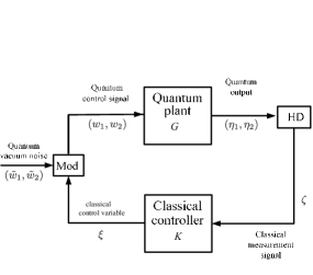
Figure 4: Measurement feedback control of a quantum system, where HD represents the homodyne detector and Mod represents the optical modulator.

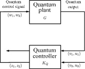
Figure 5: Quantum realization of a measurement feedback control system.

$\mathbf{Example\ 2}$: Consider a closed loop system which consists of a quantum plant $G$ and a real classical controller $K$ shown in Fig. 4. The quantum plant $G$, an optical cavity, is of the form (2.3) and is given in quadrature form by the equations

$$dq = (-\frac{\gamma}{2}q+\omega p)dt-\sqrt{\gamma}\,dw_{1}$$ (52)

$$dp = (-\frac{\gamma}{2}p-\omega q)dt-\sqrt{\gamma}\,dw_{2}$$ (53)

$$d\eta_{1} = \sqrt{\gamma}\,qdt+dw_{1}$$ (54)

$$d\eta_{2} = \sqrt{\gamma}\,pdt+dw_{2},$$ (55)

where $\omega$ is the detuning parameter, and $\gamma$ is a coupling constant. The output of the homodyne detector (Figure 4) is $\zeta=\eta_{1}$. The quantum control signal $(w_{1},w_{2})$ is the output of a modulator corresponding to the equations $dw_{1}=\xi dt+d\tilde{w}_{1}$, $dw_{2}=d\tilde{w}_{2}$, where $(\tilde{w}_{1},\tilde{w}_{2})$ is a quantum Wiener process, and $\xi$ is a classical state variable associated with the classical controller $K$, with dynamics $d\xi=-\xi dt+d\zeta$. The combined hybrid quantum-classical system $G$-$K$ is given by the equations

$$dq = (-\frac{\gamma}{2}q+\omega p-\sqrt{\gamma}\,\xi)dt-\sqrt{\gamma}\,d\tilde{w}_{1}$$

$$dp = (-\frac{\gamma}{2}p-\omega q)dt-\sqrt{\gamma}\,d\tilde{w}_{2}$$

$$d\xi = \sqrt{\gamma}qdt+d\tilde{w}_{1}$$

$$d\zeta = (\sqrt{\gamma}\,q+\xi)dt+d\tilde{w}_{1}.$$ (56)

Note that this hybrid system is an open system, and consequently the equations are driven by quantum noise. The quantum realization of the system $d\xi=-\xi dt+d\zeta$, $dw_{1}=\xi dt+d\tilde{w}_{1}$, denoted here by $K_{Q}$ is, from Example 1, given by equations (44) (with the appropriate notational correspondences). The combined quantum plant and quantum controller system $G$-$K_{Q}$ is specified by Figure 5, with corresponding closed loop equations

$$dq = (-\frac{\gamma}{2}q+\omega p-\sqrt{\gamma}\,x_{1})dt-\sqrt{\gamma}\,dv_{2}$$

$$dp = (-\frac{\gamma}{2}p-\omega q)dt-\sqrt{\gamma}\,du_{2}$$

$$dx_{1} = \sqrt{\gamma}\,qdt+dv_{2}$$

$$dx_{2} = (-x_{2}+2\sqrt{\gamma}\,p)dt+du_{2}.$$ (57)

The hybrid dynamics (56) can be seen in these equations (with $x_{1}$, $v_{2}$ and $u_{2}$ replacing $\xi$, $\tilde{w}_{1}$ and $\tilde{w}_{2}$, respectively). By the structure of the equations, joint expectations involving variables in the hybrid quantum plant-classical controller system equal the corresponding expectations for the combined quantum plant and quantum controller. For example, $E[q(t)\xi(t)]=E[q(t)x_{1}(t)]$. A physical implementation of the new closed loop quantum feedback system is shown in Figure 6.

We consider now the conditional dynamics for the cavity, [Wiseman $\&$ Milburn (2009), Bouten et al.(2007)]. Let $\hat{q}(t)$ and $\hat{p}(t)$ denote the conditional expectations of $q(t)$ and $p(t)$ given the classical quantities $\zeta(s),\xi(s),\ 0\leq s\leq t$. Then

$$d\hat{q} = (-\frac{\gamma}{2}\hat{q}+\omega\hat{p}-\sqrt{\gamma}\xi)dt+K_{q}d\nu$$ (58)

$$d\hat{p} = (-\frac{\gamma}{2}\hat{p}-\omega\hat{q})dt+K_{p}d\nu$$ (59)

where $K_{q}=\widehat{q^{2}}-(\hat{q})^{2}+1$ and $K_{p}=\widehat{qp}-\hat{q}\hat{p}$ are the Kalman gains for the two quadratures, and $\nu$ is the measurement noise (the innovations process, itself a Wiener process). The output also has the representation $d\zeta=(\sqrt{\gamma}\,\hat{q}+\xi)dt+d\nu.$ The conditional cavity dynamics combined with the classical controller dynamics leads to the feedback equations

$$d\hat{q} = (-\frac{\gamma}{2}\hat{q}+\omega\hat{p}-\sqrt{\gamma}\xi)dt+K_{q}d\nu$$ (60)

$$d\hat{p} = (-\frac{\gamma}{2}\hat{p}-\omega\hat{q})dt+K_{p}d\nu$$ (61)

$$d\xi = \sqrt{\gamma}\hat{q}dt+d\nu$$ (62)

$$d\zeta = (\sqrt{\gamma}\,\hat{q}+\xi)dt+d\nu$$ (63)

Here we can see the measurement noise $\nu(t)$ explicitly in the feedback equations. By properties of conditional expectation, we can relate expectations involving the conditional closed loop system with the hybrid quantum plant classical controller system, e.g. $E[\hat{q}(t)\xi(t)]=E[q(t)\xi(t)]$. We therefore see that the expectations involving the hybrid system, the conditional system, and the quantum plant quantum controller system are all consistent.

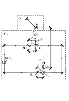
Figure 6: Quantum realization of the closed-loop system shown in Figure 5.

5 Conclusion

In this paper, we have shown that a class of classical linear stochastic systems (having a certain form and satisfying certain technical assumptions) can be realized by quantum linear stochastic systems. It is anticipated that the main results of the work will aid in facilitation the implementation of classical linear systems with fast quantum optical devices (eg. measurement feedback control), especially in miniature platforms such as nanophotonic circuits.

References

- [Anderson Vongpanitlerd (1973)] Anderson, B. D. O. Vongpanitlerd, S. (1973). Network analysis and synthesis: a modern systems theory approach. Networks Series, Prentice-Hall, Englewood Cliffs, NJ.
- [Bachor Ralph (2004)] Bachor, H. A. Ralph, T. C. (2004). A guide to experiments in quantum optics, 2nd Weinheim, Germany: Wiley-VCH.
- [Beausoleil et al.(2007)] Beausoleil, R. G. Keukes, P. J. Snider, G. S. Wang, S. Williams, R. S. (2007). Nanoelectronic and nanophotonic interconnect. Proc. IEEE, 96, 230-247.
- [Bouten et al.(2007)] Bouten, L. Handel, R. V. James, M. R. (2007). An introduction to quantum filtering. SIAM J. Control and Optimization, 46(6), 2199-2241.
- [Gardiner Zoller (2004)] Gardiner, C. Zoller, P. (2004). Quantum noise, 3rd. Berlin, Germany: Springer.
- [Gough James (2009a)] Gough, J. E. James, M. R. (2009a). The series product and its application to quantum feedforward and feedback networks. IEEE Trans. Automatic Control, 54(11), 2530-2544.
- [James et al.(2008)] James, M. R. Nurdin, H. I. Petersen, I. R. (2008). control of linear quantum stochastic systems. IEEE Trans. Automat. Control, 53, 1787-1803.
- [Merzbacher (1998)] Merzbacher, E. (1998). Quantum mechanics, 3rd. New York: Wiley.
- [Nurdin et al.(2009)] Nurdin, H.I. James, M.R. Petersen, I.R. (2009). Coherent quantum LQG control. Automatica, 45, 1837-1846.
- [Nurdin et al.(2009)] Nurdin, H. I. James, M. R. Doherty, A. C. (2009). Network synthesis of linear dynamical quantum stochastic systems. SIAM J. Control and Optim., 48, 2686-2718.
- [Nurdin (2010a)] Nurdin, H. I. (2010a). Synthesis of linear quantum stochastic systems via quantum feedback networks. IEEE Trans. Autom. Contr., 55(4), 1008-1013. Extended preprint version available at http://arxiv.org/abs/0905.0802.
- [Nurdin (2010b)] Nurdin, H. I. (2010b). On synthesis of linear quantum stochastic systems by pure cascading. IEEE Trans. Autom. Contr., 55(10), 2439-2444.
- [Nurdin (2012)] Nurdin, H. I. (2012). Network synthesis of mixed quantum-classical linear stochastic systems. In Proceedings of the 2011 Australian Control Conference (AUCC), Engineers Australia, Australia, 68-75.
- [Parthasarathy (1992)] Parthasarathy, K. (1992). An introduction to quantum stochastic calculus. Berlin, Germany: Birkhauser.
- [Wiseman Milburn (1993)] Wiseman, H. M. Milburn, G. J. (1993). Quantum theory of optical feedback via homodyne detection. Phys. Rev. Lett., 70, 548-551.
- [Wiseman Milburn (1994)] Wiseman, H. M. Milburn, G. J. (1994). All-optical versus electro-optical quantum-limited feedback. Phys. Rev. A, 49(5), 4110-4125.
- [Wiseman Milburn (2009)] Wiseman, H. M. Milburn, G. J.(2009). Quantum measurement and control. Cambridge, UK: Cambridge University Press.
- [Wang et al.(2011)] Wang, S. Nurdin, H. I. Zhang, G. James, R. M. (2011). Quantum Optical Realization of Classical Linear Stochastic Systems. In Proceedings of the 2011 Australian Control Conference (AUCC), Engineers Australia, Australia, 351-356.
- [Wang et al.(2012)] Wang, S. Nurdin, H. I. Zhang, G. James, R. M.(2012). Synthesis and structure of mixed quantum-classical linear systems. In Proceedings of the 51st IEEE Conference on Decision and Control (CDC), 1093-1098.