Star count density profiles and structural parameters
of 26 Galactic globular clusters

Abstract

We used a proper combination of high-resolution HST observations and wide-field ground based data to derive the radial star density profile of 26 Galactic globular clusters from resolved star counts (which can be all freely downloaded on-line). With respect to surface brightness (SB) profiles (which can be biased by the presence of sparse, bright stars), star counts are considered to be the most robust and reliable tool to derive cluster structural parameters. For each system a detailed comparison with both King and Wilson models has been performed and the most relevant best-fit parameters have been obtained. This is the largest homogeneous catalog collected so far of star count profiles and structural parameters derived therefrom. The analysis of the data of our catalog has shown that: (1) the presence of the central cusps previously detected in the SB profiles of NGC 1851, M13 and M62 is not confirmed; (2) the majority of clusters in our sample are fitted equally well by the King and the Wilson models; (3) we confirm the known relationship between cluster size (as measured by the effective radius) and galactocentric distances; (4) the ratio between the core and the effective radii shows a bimodal distribution, with a peak at $\sim 0.3$ for about $80$% of the clusters, and a secondary peak at $\sim 0.6$ for the remaining $20$%. Interestingly, the main peak turns out to be in agreement with what expected from simulations of cluster dynamical evolution and the ratio between these two radii well correlates with an empirical dynamical age indicator recently defined from the observed shape of blue straggler star radial distribution, thus suggesting that no exotic mechanisms of energy generation are needed in the cores of the analyzed clusters.

1. Introduction

Globular clusters (GCs) represent one of the most intensively investigated astrophysical systems in the Universe. Indeed, the comprehension of their origin and nature has implications for numerous, important fields of Astrophysics and Cosmology, from the formation of the first self-gravitating objects in the $\Lambda$CDM cosmological scenario (Kravtsov & Gnedin, 2005, see also references therein), to the theory of stellar evolution and the formation of stellar exotica (like blue stragglers and millisecond pulsars), which is made possible by the peculiarly dense and dynamically active environmental conditions of these systems (e.g., Bailyn, 1993; Bellazzini et al., 1995; Ferraro et al., 1995; Rasio et al., 2007; Ferraro et al., 2009a). Their properties also provide crucial information on the formation and evolutionary mechanisms of the Galaxy (e.g., Tremaine et al., 1975; Quinlan & Shapiro, 1990; Ashman & Zepf, 1998; Capuzzo-Dolcetta & Miocchi, 2008; Ferraro et al., 2009b; Forbes & Bridges, 2010), as well as on the processes characterizing the dynamical evolution of collisional systems (e.g., Meylan & Heggie, 1997; Ferraro et al., 2012).

Despite the undoubted importance of precisely and accurately determining their properties, most of the Galactic GC structural and morphological parameters are still derived from surface brightness (SB) profiles extracted from mid-80’s CCD images and, in a minority of cases, from star counts on photographic plates mostly dating back to late 60’s–70’s (Trager et al., 1995). Even the most recent parameter compilations (McLaughlin & van der Marel, 2005, hereafter MvM05; Wang & Ma 2013 for M31 clusters) are based on SB measurements. Indeed, SB profiles are known to suffer from possible bias due to the presence of very bright stars (see, e.g., Noyola & Gebhardt, 2006, for the discussion of methods trying to correct for this problem). Instead, every star has the same “weight” in the construction of the number density profile and no bias is therefore introduced by the presence of sparse, bright stars. For this reason, resolved star counts represent the most robust way for determining the cluster density profiles and structural parameters (see, e.g., Lugger et al., 1995; Ferraro et al., 1999b, 2003). In spite of these advantages, however, only a few studies regarding individual or very small sets of clusters (e.g. Salinas et al., 2012) have been performed to date, while, to our knowledge, no catalogs of star count profiles sampling the entire cluster radial extension can be found in the literature. This is essentially due to the fact that the construction of complete samples of stars both in the highly crowded central region and in the outermost part of clusters is not an easy task. It requires the proper combination of high-resolution photometry sampling the cluster centers and high-precision wide-field imaging of the external parts. In particular, an appropriate coverage of even the regions beyond the tidal radius is necessary to get a direct estimate of the level of contamination from background and foreground Galactic field stars.

It is worth noting that both the inner and the outer portions of the profile provide crucial information on the structure of the cluster. In fact, the central part constrains the core radius, the central density, and also the possible existence of a power-law cusp (Noyola & Gebhardt, 2006, 2007) due to the post-core collapse state of the system (Djorgovski & King, 1986; Trenti et al., 2010), or to the presence of an Intermediate-Mass Black Hole (IMBH; Bahcall & Wolf, 1976; Baumgardt et al., 2005; Miocchi, 2007, but see also Vesperini & Trenti 2010). The external portion provides information on the possible presence of tidal tails and structures well outside the cluster Roche lobe, that are indeed observed in a growing number of GCs (see, e.g., Leon et al., 2000; Testa et al., 2000; Odenkirchen et al., 2003; Belokurov et al., 2006; Koch et al., 2009; Jordi & Grebel, 2010; Sollima et al., 2011). The influence of escaped stars (either originated by two-body internal relaxation or by tidal stripping due to the external field) on the outer density profile makes more and more questionable the use of the widely employed King (1966) model (see, e.g., the catalogs of Djorgovski, 1993; Pryor & Meylan, 1993; Trager et al., 1995; Harris, 1996, 2010 version, hereafter H10, and MvM05). In this model, the tidal effect is imposed by construction with a sharp cutoff of the Maxwellian distribution at the “limiting radius”, while many clusters seem to show a radial density that drops towards the background level much more smoothly than the King model predicts, even following a scale-free power-law profile (Grillmair et al., 1995; Jordi & Grebel, 2010; Küpper et al., 2010; Carballo-Bello et al., 2012; Zocchi et al., 2012, but see also Williams et al. 2012 for a recently proposed “collisionless” model). For this reason, MvM05 tested the Wilson (1975) model to reproduce the SB profile of Milky Way and Magellanic Clouds GCs, finding that most of the latter and $\sim 80\%$ of the Galactic sample are better fitted by this alternative model, which gives a smoother cutoff at the limiting radius. However, this could be due to a not appropriate coverage of the cluster external region and therefore a not accurate background decontamination. Recently, Carballo-Bello et al. (2012) used wide-field star count data to study the very outer parts of 19 Galactic GCs in the inner-halo, showing that King and power-law models both provide reasonable fits to the observations in most of the cases, though the latter gives a better representation for $\sim 2/3$ of their sample. Finally, a substantial equivalence of King and Wilson models in representing the structure of 79 globulars in M31 was found by a very recent collection of HST SB profiles (Wang & Ma, 2013).

In this paper we provide the first homogeneous catalog of star count density profiles and derived structural parameters, for a sample of 26 Galactic GCs. Both King and Wilson models are used to fit the observations. We specifically focus on apparently “normal” GCs, showing a star count central density with no significant deviations from a flat behavior (hence no post core-collapsed systems or clusters with a central density cusp have been included in the sample). The paper is organized as follows: in Sect. 2 we give some details about the construction of the observed density profiles; in Sect. 3 the adopted self-consistent models are outlined and defined and a description of the best-fitting procedure is given; finally, conclusive remarks are presented in Sect. 4.

2. Observed star count profiles

In all cases (but the loosest object, NGC 5466), the cluster central regions have been sampled with high-resolution HST observations, thus properly resolving stars even in the most crowded environments. These data have been combined with complementary sets of wide-field ground-based observations in order to cover the external parts of the target clusters, thus sampling the entire radial extension and, in most of the cases, even beyond (see, e.g., Lanzoni et al., 2007a, b; Dalessandro et al., 2008, and references therein). The projected density profile of each cluster has been determined from direct star counts in concentric annuli around the gravity center($C_{\mathrm{grav}}$). While the procedure is described in detail in each specific paper (see references in Table 2), here we quickly summarize the main steps.

Table 1Centers of gravity

NGC name	$\alpha$	$\delta$	$\sigma_{\alpha,\delta}$	Ref.
	(h:m:s)	($\textrm{deg}:\arcmin:\arcsec$)	(″)
104 (47Tuc)	$00:24:05.71$	$-72:04:52.20$	$0.5$	1
288	$00:52:45.24$	$-26:34:57.40$	$1.8$	1, 2
1851	$05:14:06.755$	$-40:02:47.47$	$0.1$	1
1904 (M79)	$05:24:11.09$	$-24:31:29.00$	$0.5$	3
2419	$07:38:8.47$	$+38:52:55.0$	$0.5$	4
5024 (M53)	$13:12:55.18$	$+18:10:06.1$	$0.5$	1
5272 (M3)	$13:42:11.38$	$+28:22:39.1$	$1$	1
5466	$14:05:27.25$	$+28:32:01.8$	$2$	1
5824	$15:03:58.637$	$-33:04:05.90$	$0.2$	1
5904 (M5)	$15:18:33.214$	$+02:04:51.80$	$0.2$	1
6121 (M4)	$16:23:35.03$	$-26:31:33.89$	$1$	1
6205 (M13)	$16:41:41.21$	$+36:27:35.61$	$0.4$	1
6229	$16:46:58.74$	$+47:31:39.53$	$0.1$	5
6254 (M10)	$16:57:8.92$	$-04:05:58.07$	$1$	6
6266 (M62)	$17:01:12.98$	$-30:06:49.00$	$0.2$	1
6341 (M92)	$17:17:07.43$	$+43:08:09.26$	$0.1$	1
6626 (M28)	$18:24:32.73$	$-24:52:13.07$	$0.7$	1
6809 (M55)	$19:39:59.84$	$-30:57:50.81$	$1$	1
6864 (M75)	$20:06:4.85$	$-21:55:17.85$	$0.5$	7
7089 (M2)	$21:33:26.96$	$-00:49:22.97$	$1$	8
AM 1	$03:55:02.5$	$-49:36:53.2$	$1$	9
Eridanus	$04:24:44.7$	$-21:11:13.9$	$1$	9
Palomar 3	$10:05:31.56$	$+00:04:21.74$	$2$	9
Palomar 4	$11:29:16.47$	$+28:58:22.38$	$>2$	9
Palomar 14	$16:11:00.8$	$+14:57:27.8$	$1$	10
Terzan 5	$17:48:04.85$	$-24:46:44.6$	$1$	11

Note. — Centers of gravity and references for the star count surface density profiles of all the GCs in our sample. The $\alpha$ and $\delta$ coordinates of $C_{\mathrm{grav}}$ are referred to epoch J2000. Their uncertainty (the same in $\alpha$ and in $\delta$) is given in column 4, in units of arcseconds.

References. — (1) this work; (2) Goldsbury et al. (2010); (3) Lanzoni et al. (2007b); (4) Dalessandro et al. (2008); (5) Sanna et al. (2012): (6) Dalessandro et al. (2011); (7) Contreras et al. (2012); (8) Dalessandro et al. (2009); (9) Beccari et al. (2012); (10) Beccari et al. (2011); (11) Lanzoni et al. (2010).

At odds with many previous studies that adopts as cluster center the position of the SB peak, for each GC in our sample we computed $C_{\mathrm{grav}}$ from star counts, thus to avoid any possible bias introduced by the presence of a few bright stars. $C_{\mathrm{grav}}$ is determined by averaging the right ascension ($\alpha$) and declination ($\delta$) of all stars lying within a circle of radius $r$. Depending on the available datasets and the cluster characteristics, in every GC we selected the optimal range of stellar magnitudes, thus to have enough statistics and avoid spurious effects due to photometric incompleteness (that especially affects the innermost, crowded regions). The radius $r$ is chosen as a compromise between including the largest number of stars and avoiding the gaps of the instrument CCDs. The adopted values of $r$ always exceed the cluster core radius as quoted by H10, thus to be sensitive to the portion of the profile where the slope changes and the density is no more uniform. The search for $C_{\mathrm{grav}}$ starts from a first-guess center and stops, within an iterative procedure, when convergence is reached. As a further consistency check, the center was also determined by averaging the stellar coordinates weighted by the local number density, in a way similar to that outlined by Casertano & Hut (1985) in the context of cluster $N$-body simulations (see Lanzoni et al., 2010, for more details). The two estimates turn out to be consistent within the errors, as it is indeed expected in the case of flat-core profiles (like those included in the present sample). The values of $C_{\mathrm{grav}}$ adopted in the present paper are listed in Table 2.

Figure 1 shows the differences between the coordinates of the cluster centers of Table 2 and those quoted in Goldsbury et al. (2010) or in H10 for those GCs not included in Goldsbury’s sample. Differences in both right ascension and declination are always smaller than $\sim 4\arcsec$, but for two GCs, namely Palomar 3 and Palomar 4. These are two very loose clusters, with extremely low stellar densities even within the core region. Hence, the determination of their center is much more difficult, as also testified by the quite large resulting uncertainties ($\sigma_{\alpha,\delta}\geq 2\arcsec$). In addition, the center of Palomar 4 quoted in H10 has been determined from scanned plates (Shawl & White, 1986) and can therefore be inaccurate. In any case, it is worth noticing that in the case of such loose GCs, with relatively large core, no significant impact on the density profile is expected from a few arcsecond erroneous positioning of $C_{\mathrm{grav}}$.

Figure 1.— Differences between our determination of the coordinates of each GC center (Table 2) and that quoted in the literature (filled squares: Goldsbury et al., 2010, open squares: H10 for GCs not included in the Goldsbury et al. sample). Reported are the names of clusters showing a difference $>4\arcsec$.

The projected number density profile, $\Sigma_{*}(r)$, is determined by dividing the entire data-set in $N$ concentric annuli, each one partitioned in four subsectors (only two or three subsectors are used if the available data sample just a portion of the annulus). The number of stars in each subsector is counted and the density is obtained by dividing this value by the sector area. The stellar density in each annulus is then obtained as the average of the subsector densities, and the uncertainty is estimated from the variance among the subsectors. Also in this case, only stars within a limited range of magnitudes are considered in order to avoid spurious effects due to photometric incompleteness. As described above, the innermost portion of the profile is computed by using high-resolution HST data, while the outer part is obtained from wide-field ground-based observations. The two portions are normalized by using the annular regions not affected by incompletness that are in common between the two data-sets.

The observed stellar density profiles are shown in Figure 2 (open symbols) for the 26 GCs in the sample. In most of the cases the collected dataset covers the entire cluster extension, reaching the outermost region where the Galactic field stars represent the dominant contribution with respect to the cluster. The spatial distribution of field stars is approximately uniform on the considered radial bin scales, and this produces a sort of “background plateau” in the outermost region of the star count profile. Hence, by averaging the values of the $N_{\mathrm{BG}}$ points in this plateau, we estimate the Galaxy background contamination to the cluster density (short-dashed lines in Figure 2). The decontaminated cluster profile, obtained after subtracting the Galaxy background level, is finally shown as black symbols in the figure. As apparent, after the field subtraction, the profile remains unchanged in the inner and most populous regions, while the cluster data points can be significantly below the background level in the most external parts. As a consequence, the accurate measure of the background level is crucial for the reliable determination of the outermost portion of the profile.

Figure 2.— Observed star count profiles and corresponding best-fit King (solid curve) and Wilson (long-dashed curve) models. For each cluster, in the upper panel the open circles mark the observed star count surface density profile, while solid circles correspond to the profile after the subtraction of the the Galactic field background density estimate (short-dashed line, if available). The lower section of each panel shows the residuals between the (decontaminated) observed profile and the model (K=King, W=Wilson) with the lowest value of $\chi^{2}_{\nu}$. The error bars of the decontaminated points include the uncertainty in the background determination.

Figure 2.— (Continued)

Figure 2.— (Continued)

Figure 2.— (Continued)

Figure 2.— (Continued)

Figure 2.— (Continued)

Figure 2.— (Continued)

3. Models

To reproduce the observed star density profiles and thus to derive the cluster structural parameters, we considered both the King (1966) and the Wilson (1975) models (see also Hunter, 1977), in the isotropic, spherical and single-mass approximation. These models (the former, in particular) have been widely used to represent stellar systems like GCs, that are thought to have reached a state of (quasi-)equilibrium similar to the one attained by gases following the Maxwellian distribution function. Besides the generally good agreement with observations (but see the discussion in Williams et al., 2012) and its valid physical motivations, the King model has been also derived from a rigorous statistical mechanics treatment (Madsen, 1996).

Qualitatively, the projected density profiles of the King and Wilson models are characterized by a constant value in the innermost part (the “core”), and a decreasing behavior outwards, with the Wilson model showing a more extended outer region (see Appendix A and, e.g., Figures 9 and 10 in MvM05, ). In both cases the density profiles constitute a one-parameter family. This means that the profile shape is uniquely determined by the dimensionless parameter $W_{0}$, which is proportional to the gravitational potential at the center of the system. In practice, the higher $W_{0}$ the smaller is the cluster core with respect to the overall size of the system. More details about these models are presented in Appendix A.

Several characteristic scale-lengths can be defined in both model families. Some of them have a precise theoretical definition, but no observational correspondence; some other are commonly adopted in observational studies, but suffer from some degree of arbitrariness when measured from the available data. However, since numerical models have become increasingly more realistic, much attention has to be paid to give clear and unambiguous definitions of these parameters so as to allow a closer and meaningful comparison between theoretical and observational results (see e.g. Hurley, 2007; Trenti et al., 2010).

Here we consider a number of different scale radii, thus to allow the widest possible use and the connection between theory and observations. We call “scale radius” ($r_{0}$) the characteristic length parameter of the model, which most authors refer to as “King radius” in the case of the King family. This must not be confused with the “core radius” ($r_{\mathrm{c}}$), which is operatively defined as the radius at which the projected stellar density $\Sigma_{*}(r)$ drops to half its central value (in other studies the SB is considered instead of $\Sigma_{*}$). The values of the scale and core radii are similar, their difference tending to zero for $W_{0}\to\infty$.

We define the “half-mass radius” ($r_{\mathrm{hm}}$), as the radius of the sphere containing half of the total cluster mass. Of course, $r_{\mathrm{hm}}$ cannot be directly observed and we therefore consider also the “effective radius” ($r_{\mathrm{e}}$), commonly defined as the radius of the circle that in projection includes half the total integrated light. In the case of star counts (instead of SB) profiles, the total integrated light corresponds to the integral of the number density profile over all radii (i.e. the total number of observed stars). For various reasons (including that, with respect to other characteristic scale-lengths like $r_{\mathrm{c}}$, it weakly varies during the cluster evolution) this radius is commonly adopted to measure the GC size (see, e.g., Spitzer & Thuan, 1972; Lightman & Shapiro, 1978; Murphy et al., 1990).

Finally, the “limiting radius” ($r_{\ell}$) is the model cutoff radius, at which the density $\Sigma_{*}$ goes to zero. This is often and rather improperly called the “tidal radius”, even if it is not directly and trivially related to the tidal effect of the Galactic field (see also Binney & Tremaine, 1987; Küpper et al., 2010). The logarithm of the ratio between the limiting and the scale radii is called the “concentration parameter”, $c\equiv\log(r_{\ell}/r_{0})$. In the considered models there is a one-to-one relation between the value of $W_{0}$ and that of $c$, with the cluster concentration increasing as $W_{0}$ increases (see Figure 9). Since the Wilson model shows a more extended outer region, the half-mass, effective and limiting radii, and, as a consequence, also the concentration parameter, are appreciably larger than in the King model for any fixed scale radius $r_{0}$ (see Appendix A, and, e.g., MvM05, ).

3.1. Best-fitting procedure

The search for the best-fit to the observed surface density profiles is performed by exploring a pre-generated grid of $n$ models with the shape parameter $W_{0}$ ranging from 1 to 12 and stepped by $0.05$, both in the King and in the Wilson cases. The corresponding concentration parameters vary between 0.5 and 2.74 in the King case, and between 0.78 and 3.52 for the Wilson model. The model density profiles are finely sampled in radius: about 100 logarithmically spaced bins are used, so that linear interpolation yields accurate estimates at any radius. In order to fit a given observed (and background decontaminated) profile, the entire grid of models is scanned and for each value of $W_{0,i}$ (with $i=1,n$) a direct searching algorithm finds the two scaling parameters $r_{0,i}$ and $\Sigma_{*,i}(0)$ that minimize the sum of the unweighted squares of the residuals and evaluates the corresponding $\chi^{2}$ value ($\chi^{2}_{\mathrm{min},i}$). At the end of the procedure, the best-fit model is defined as the one corresponding to the lowest value among all the obtained $\chi^{2}_{\mathrm{min},i}$ (let us indicate it as $\chi^{2}_{\mathrm{best}}$).

Results are listed in Table 2. For each cluster, both the King and the Wilson best-fit models are given. The quality of the fit is reported in the third column of the table in terms of the reduced $\chi^{2}$ ($\chi^{2}_{\nu}$), i.e. the value of $\chi^{2}_{\mathrm{best}}$ divided by the number of the fit degrees of freedom. This is equal to $N-N_{\mathrm{BG}}-3$, where $N$ is the total number of observed points, $N_{\mathrm{BG}}$ is the number of points used to evaluate the Galaxy background contamination (see Sect. 2), and 3 quantities (two scale parameters and $W_{0}$) are evaluated by the best-fit. As apparent, for many GCs the two models give an approximately equivalent fit to the data, while in a few cases the observations are significantly better reproduced by one of the two (see Sect.4).

The 1-$\sigma$ confidence intervals of the best-fitting parameters (see Table 2) are estimated from the distribution of the $\chi^{2}_{\mathrm{min},i}$ values, in line with the method of the $\Delta\chi^{2}$ described, e.g., in Press et al. (1988). From this distribution we select the sub-set of models with $\chi^{2}_{\mathrm{min},i}\leq\chi^{2}_{\mathrm{best}}+1$. Then, the 1-$\sigma$ uncertainty range of a parameter is assumed to be equal to the maximum variation of that parameter within this sub-set of models (as it is done in MvM05, ). In some cases, this procedure yields large uncertainty ranges either because the fit is not very good (for example, in the case of the King model fit of NGC 2419), or because there is a relatively small amount of data points (as in the cases of Palomar 3 and Palomar 4). Moreover, as can be appreciated in Table 2, the uncertainty limits are often asymmetric with respect to the best-fit value.

Given the importance of a correct evaluation of the Galactic background for a proper definition of the cluster density profile (Sect. 2), we tried to estimate the sensitivity of the fitting procedure to this quantity. In general, we found that a change in the background level can significantly affect only the one/two most external points considered in the fit procedure. This can possibly change the best-fit value of $W_{0}$ (and hence of $c$), while the scale radius is essentially unaffected. However in most of the cases the large radial coverage of our data-sets guarantees a solid evaluation of the background level, and only in a few clusters (see footnotes in Table 2) the exclusion of the last data point allows a considerable improvement of the fit, possibly suggesting that the Galactic background could be underestimated for these systems.

4. Discussion

Figure 2 shows the observed density profiles and the results of the fitting procedure for all the program clusters. The best-fit King and Wilson profiles are plotted as solid and long-dashed lines, respectively. The lower panel shows the residuals with respect to the model that provides the lowest value of $\chi^{2}_{\nu}$, and, in the following, we call K-type (or W-type) clusters those for which this model is the King (or Wilson) one. Our analysis classifies $50\%$ of GCs in our sample as W-type. This percentage is smaller than that found by MvM05 for their Galactic sample, but the different size of the two samples should be taken into account. In fact, a change of classification for just a few clusters in our case would suffice to significantly alter the overall percentage.

The collected catalog offers the possibility of a meaningful comparison with results obtained from SB profiles. We noted, for instance, that three clusters in common with our sample (namely NGC 1851, M13 and M62) show hints of a SB central cusp in the work of Noyola & Gebhardt (2006). No evidence of such a feature is instead found in the star density profile shown in Fig. 2. A close inspection of the SB profiles published in Noyola & Gebhardt (2006) reveals that, although their data sample a region more internal with respect to ours, a deviation from a flat core behavior should be already appreciable in the region sampled by our observations, at least in correspondence to our innermost data point. Indeed this disagreement could be the manifestation of the typical bias affecting the SB profiles, where a group of a few bright giants can produce a spurious enhancement of the SB, not corresponding to a real overdensity of stars.

Comparing our results with those presented by MvM05 for the 23 clusters in common (i.e., all clusters in our sample, but NGC 6626, Eridanus and Terzan 5), we find that the same type of best-fit model is obtained for 15 GCs, five (ten) of which are best fitted by a King (Wilson) model in both studies. For the remaining eight GCs the two works provide different best-fit model (seven are K-type in our study and W-type in MvM05, and vice-versa for the remaining one), at least formally. Indeed, significant differences ($\gtrsim 30\%$) between the quoted $\chi^{2}_{\nu}$ values are found only for two clusters, namely M2 and M10, which are of K-type in our study and of W-type in MvM05. A detailed inspection of Figure 2 shows that the discrimination between the two types of model adopted here is often driven by the last, background-subtracted, points. On the other hand, the datasets used by MvM05 are less radially extended (see their Figure 12) and the last points of their SB profiles are not corrected for the Galactic background level. Therefore, we can reasonably state that the aforementioned differences in the best-fit model classification can be ascribed to a residual background contamination of the MvM05 profiles.

In Figures 3 and 4 we compare some relevant structural parameters derived in our study and in MvM05. Fig. 3 refers to the 15 clusters for which the best-fit model is of the same type in both studies, the left- and right-hand panels concerning, respectively, the five K-type and the ten W-type GCs. Fig. 4, instead, refers to the eight clusters for which the best-fit model is of different type: in the left-hand panels we compare the structural parameters obtained from King models, while the right-hand panels refer to Wilson models. In general, a good agreement is found between the parameters derived in our work and in MvM05. The largest differences are found mostly for the the Wilson best-fit limiting radius, which, in turn, also affects the values of $c$ and $W_{0}$. These differences are reasonably expected, since the Galactic background seems not well sampled in MvM05 for most of the clusters in common. This could explain why the majority of our estimates of $r_{\ell}$ (and, in turn, of $W_{0}$ and $c$) are larger than those quoted in MvM05, especially for Wilson best-fit profiles (because of the more extended envelope).

Figure 3.— Comparison between various best-fit structural parameters as obtained in our study and in MvM05, for the 15 clusters that are best-fitted by the same type of model in both works. Results for the five K-type GCs and the ten W-type GCs are shown, respectively, in the left-hand and in the right-hand sides of each panel (see labels). From top-left to bottom-right the considered structural parameters are: $W_{0}$, $r_{0}$ $r_{\ell}$, $c$, $r_{\mathrm{e}}$, and $r_{\mathrm{c}}$ (see x-axis labels). The relative difference $\epsilon\equiv(\hat{p}-p)/p$ between the value of the generic parameter quoted by MvM05 ($\hat{p}$) and the corresponding value obtained in our analysis ($p$) is plotted as a function of $p$.

Figure 4.— The same as in Fig. 3, but for the eight clusters which are have different type of best-fit model in the two studies: the structural parameters corresponding to the King model fitting are shown in the left-hand side of each panel, those from the Wilson fitting are shown in the right-hand sides.

In order to provide a quantitative estimate of the ability of the fitting procedure to clearly discriminate between the two King and Wilson models, we used the relative difference between the reduced $\chi^{2}$, i.e. the quantity $\Delta\equiv(\chi^{2}_{\mathrm{W}}-\chi^{2}_{\mathrm{K}})/(\chi^{2}_{\mathrm{W}}+\chi^{2}_{\mathrm{K}})$ (as in MvM05, ). Thus, $\Delta=0$ indicates that the two models provide fits of the same quality, while $\Delta\simeq 1$ means that the King fit is substantially better than the Wilson one, and vice-versa for $\Delta\simeq-1$.

In Fig. 5 we plot $\Delta$ as a function of $r_{\mathrm{last}}/r_{\mathrm{e}}$, where $r_{\mathrm{last}}$ is the radius of the outermost point of the decontaminated density profile. The quantity along the abscissa is a measure of how many effective radii are sampled by the observations. Note that in our catalog all clusters (but 47Tuc, NGC 1851 and Eridanus) are sampled out to where the Galactic field becomes dominant. Hence $r_{\mathrm{last}}/r_{\mathrm{e}}$ is a measure of the actual extension of each cluster (apart from the three aforementioned clusters for which it represents only the radial extension sampled by the observations). As in MvM05 (their Fig. 14, bottom-right panel), we find that the discrimination becomes more solid in more extended clusters (for $r_{\mathrm{last}}/r_{\mathrm{e}}\gtrsim 6$). This is indeed expected, since the King and Wilson model profiles differ only in the external regions. Interestingly, however, K-type clusters are found also for large values of $r_{\mathrm{last}}/r_{\mathrm{e}}$, thus indicating that the classification in King or Wilson type is linked to intrinsic properties of the systems and not due to observational biases (like an insufficient radial sampling of the profile). Finally, a hint of a trend toward best-fit Wilson models ($\Delta\sim-1$) for increasing radial extension of the cluster seems to be present, but the number of clusters in our sample is too small to draw a firmer conclusion concerning this trend. As to this point, it is also important to notice that King models have an intrinsic upper limit of $\sim 13$ for $r_{\mathrm{last}}/r_{\mathrm{e}}$ (see Fig.9, second panel from the bottom, and note that $r_{\mathrm{last}}\leq r_{\ell}$ by definition), while Wilson models allow to fit clusters characterized by larger values of this ratio ($\lesssim 145$).

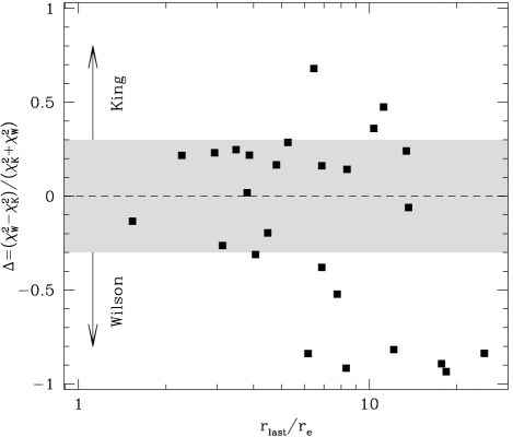
Figure 5.— Goodness of the Wilson fit with respect to the King fit (expressed as the relative difference between the respective $\chi^{2}_{\nu}$) for our GC sample as a function of the observed radial extent of the cluster (see text). Points with $\Delta>0$ correspond to GCs better fitted by King models, those with $\Delta<0$ are of W-type. The shaded region (where $|\Delta|\leq 0.3$) includes clusters whose W- and K-type best-fit profiles turn out to be practically equivalent at a “visual inspection”.

However, it is interesting to note that the large majority of the cluster lies around $\Delta=0$, thus indicating a not significant difference in the quality of the fit between the two kinds of models. To be conservative, we have highlighted as a gray strip a region ($-0.3<\Delta<0.3$) where the $\Delta$ parameter does not allow a clear-cut preference in the fitting procedure for either King or Wilson models, in the sense that, by a visual inspection, they fit equally well the profile, especially in the inner part.

The top panel of Fig. 6 shows the $\Delta$ parameter as a function of the galactocentric distance ($R_{\mathrm{g}}$). The values of $R_{\mathrm{g}}$ have been taken from H10, while the distance moduli are from Ferraro et al. (1999a), with the exception of Terzan 5 (for which we adopted the distance quoted by Valenti et al., 2007) and all GCs not included in these works (for which the distances quoted in H10 have been assumed). According to the discussion above, we have highlighted the clusters with an “equivalent” classification as gray squares. Even with these caveats, we notice that there is a group of clusters between $10$ and $30$ kpc for which Wilson models can fit the data definitely better than King models. In the same range of galactocentric distances there are also clusters best fitted by King models and clusters for which the two models provide fits of similar quality. Different orbital properties (and the ensuing differences in the cluster dynamical evolution) might be responsible for the existence of these different groups of clusters.

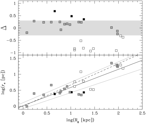
Figure 6.— Upper panel: the $\Delta$ parameter of Fig. 5 plotted as a function of the galactocentric distance of each cluster. Lower panel: clusters size (effective radius) vs. galactocentric distance; the solid line corresponds to the linear least squares fit $\log(r_{\mathrm{e}}/\mathrm{pc})=0.57\log(R_{\mathrm{g}}/\mathrm{kpc})+0.018$, with the uncertainty region enclosed by the two dotted lines (the dashed line is the $R_{\mathrm{g}}^{2/3}$ relation; see van den Bergh, 2011). Solid and open dots are clusters clearly best-fitted by King and Wilson model, respectively, while gray squares mark clusters of “equivalent” type classification ($|\Delta|\leq 0.3$, the gray strip in the upper panel).

The analyzed sample has been used also to test the existence of a relation between the cluster size (usually measured with $r_{\mathrm{e}}$) and the galactocentric distance (see, e.g., van den Bergh, 2011; Madrid et al., 2012, and references therein). The result is shown in the bottom panel of Fig. 6, where the $r_{\mathrm{e}}$ values are taken from the type of model giving the lowest $\chi^{2}_{\nu}$. A correlation is visible (the Pearson’s coefficient is $\simeq 0.84$), with a slope slightly smaller than $2/3$ as derived by van den Bergh (2011, using data from the H10 catalog), but still compatible within the uncertainties. The scaling relation we obtain is

$$\frac{r_{\mathrm{e}}}{\textrm{pc}}\sim(1.0\pm 0.2)\left(\frac{R_{\mathrm{g}}}{\textrm{kpc}}\right)^{0.57\pm 0.07}.$$ (1)

A qualitatively similar trend has been recently observed also for a sample of GCs in M31 (Wang & Ma, 2013). The importance of the role played by the external Galactic field in determining this relation (e.g. van den Bergh, 1994) has been recently suggested on more rigorous theoretical grounds (Ernst & Just, 2013).

Following van den Bergh (2011, 2012), we also tested the existence of a few relations between cluster structural properties that might also help explaining the observed scatter around the relation expressed by Eq. (1). In particular, we studied the behavior of $r_{\mathrm{e}}$, $c$ and the metallicity [Fe/H] as a function of both the total absolute magnitude $M_{V}$ and the parameter $0.57\log R_{\mathrm{g}}-\log r_{\mathrm{e}}$ quantifying the deviations from Eq. (1). We adopted the integrated magnitudes quoted by H10, while reddening parameters and metallicities have been taken from Ferraro et al. (1999a), or from H10 for the GCs not included in that work. No significant correlations are found, independently of the type of best-fit model, thus confirming the results of van den Bergh (2011, 2012) and his suggestion that the large observed scatter is probably due to the spread of cluster orbital parameters, not being correlated with other structural/chemical features.

Finally, our catalog allows us to discuss the distribution of the ratio between the core radius and the effective radius ($r_{\mathrm{c}}/r_{\mathrm{e}}$). Standard dynamical models of GCs suggest that the value of this parameter tends to decrease during the cluster long-term evolution driven by two-body relaxation, until an energy source (e.g. primordial binaries or three-body binaries) halts the core contraction and this ratio settles to a value determined by the efficiency of the energy source (see e.g. Heggie & Hut, 2003). On the other hand it has been shown that the presence of exotic populations, such as stellar mass black holes or an IMBH in the core of GCs, may prevent the decrease of this ratio and, possibly, cause its increase (e.g. Merritt et al., 2004; Baumgardt et al., 2005; Heggie et al., 2007; Mackey et al., 2008; Trenti et al., 2010). For this reason, such a ratio has been used for preliminary selection of GCs that might harbor an IMBH, e.g. in deep radio imaging studies (Strader et al., 2012).

The histogram in Fig. 7 shows the distribution of $r_{\mathrm{c}}/r_{\mathrm{e}}$ as turns out from our GC sample. Indeed, the distribution appears to be bimodal or at least significantly tailed toward high values. In order to provide a quantitative statistical support to this appearance we reconstruct the distribution of $r_{\mathrm{c}}/r_{\mathrm{e}}$ using the Kernel Density Estimation (Silverman, 1986; Sheather & Jones, 1991; Scott, 1992). This technique is essentially a generalized histogram, that allows to non-parametrically recover the underlying distribution of a variable based on a sample of $n$ points by adding together $n$ bump functions (kernels) centered on each point. Fig. 7 shows the probability-density distribution thus obtained: a qualitative indication of bimodality emerges. The probability density is well-reproduced by the superposition of two Gaussian distributions with the same standard deviation, suggesting that two different populations exist (a more compact one with $r_{\mathrm{c}}/r_{\mathrm{e}}$ peaked around $0.26$, and a less compact group peaked around $0.62$) and are barely resolved due to observational errors on both parameters. We run a Shapiro-Wilk normality test (Royston, 1982a, b) obtaining that, under the null-hypothesis of normality, the $p$-value for our data is relatively low ($p=0.099$). While this is not, by itself, a strong indication that the null-hypothesis of the data coming from a single normal distribution is to be rejected, we also note that the skewness and kurtosis of the distribution, as estimated from the sample, are $0.57$ and $-0.86$ respectively (as opposed to an expected value of $0$ in the normal case). Then, despite the not very large number of clusters in our sample, we can conclude against normality, arguing that the underlying distribution is bimodal or at least heavy tailed.

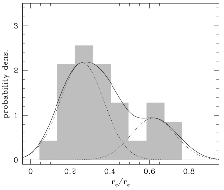
Figure 7.— Histogram of the probability density distribution of the best-fit $r_{\mathrm{c}}/r_{\mathrm{e}}$ values for the GCs in our sample. The solid line corresponds to the underlying probability density function as deduced from Kernel Density Estimation. The dotted lines represent two Gaussians with the same standard deviation ($\sigma=1.1$) that well fit, by eye, the two observed maxima.

It is interesting to notice that the main peak at $\sim 0.26$ coincides with the value assumed by $r_{\mathrm{c}}/r_{\mathrm{e}}$ during a large fraction of cluster evolution in the $N$-body simulations of Trenti et al. (2010). As for the group characterized by larger values of $r_{\mathrm{c}}/r_{\mathrm{e}}$, these might be dynamically younger clusters, with values of $r_{\mathrm{c}}/r_{\mathrm{e}}$ corresponding to those imprinted by formation and early evolution processes. In order to probe this, in Fig. 8 we plot $r_{\mathrm{c}}/r_{\mathrm{e}}$ as a function of the “dynamical clock” parameter, which has been recently proposed as an empirical indicator of the cluster dynamical age (Ferraro et al., 2012). The well defined trend between $r_{\mathrm{c}}/r_{\mathrm{e}}$ and this dynamical-age indicator does indeed seem to lend support to this interpretation. As discussed, for example, in Trenti et al. (2010), large values of $r_{\mathrm{c}}/r_{\mathrm{e}}$ for dynamically old clusters might require the presence of an IMBH as an energy source in the cluster core. Although the characterization of the dynamical age of a cluster is not simple and much caution is needed in the interpretation of these trends, our analysis and in particular the absence of any clusters with large dynamical age (large $r_{\mathrm{min}}/r_{\mathrm{c}}$) and large values of $r_{\mathrm{c}}/r_{\mathrm{e}}$ suggests that no IMBH is required in any clusters of our sample.

Figure 8.— Core to effective radii ratio as a function of the Ferraro et al. (2012) “dynamical clock” parameter, plotted for the 14 clusters in common with this study, plus two additional cases, namely NGC 5466 (Beccari et al., in prep.) and NGC 5824 (Sanna et al., in prep.). Reported is the linear least square fit (solid line).

Appendix A Some details on the parametric models

The spherical and single-mass King (1966) model in the isotropic form adopts a stars energy distribution function (DF), $f_{\mathrm{K}}(E)$, of the form

$$f_{\mathrm{K}}(E)\propto\left\{\begin{array}[]{ll}\exp(-E/\sigma^{2})-1,&\textrm{if $E<0$,}\\ 0,&\textrm{if $E\geq 0$,}\end{array}\right.$$ (A1)

with $\sigma$ being a velocity scale parameter and $E$ the star total energy. This DF abruptly cuts off at energy $E=0$. In the isotropic Wilson (1975) model the DF is slightly changed as:

$$f_{\mathrm{W}}(E)\propto\left\{\begin{array}[]{ll}\exp(-E/\sigma^{2})-1+E/\sigma^{2},&\textrm{if $E<0$,}\\ 0,&\textrm{if $E\geq 0$.}\end{array}\right.$$ (A2)

It eliminates the discontinuity of the first derivative that $f_{\mathrm{K}}(E)$ exhibits at $E=0$ and it decreases more slowly than $f_{\mathrm{K}}(E)$ for increasing energy, thus going to zero more smoothly. In practice, the DF of Eq. (A2) produces a more extended envelope and a larger effective radius.

More details and comparison between these distribution functions can be found in Sect. 4.1 of MvM05. Here, we just want to remind that in the numerical solution of the Poisson integration needed to generate self-consistent parametric models of a given DF, it is quite useful to express the volume density as a function of the gravitational potential $\Psi(r)$:

$$\rho(r)\propto\int f(\Psi(r)+v^{2}/2)v^{2}\mathrm{d}v$$ (A3)

(under the assumption of isotropic velocity ${\mathbf{v}}$ distribution and with $v=|{\mathbf{v}}|$). Indeed, for the Wilson model the DF in Eq.(A2) leads to

$$\rho(W)=\rho_{1}\left[\mathrm{e}^{W}\mathrm{erf}(\sqrt{W})-(4W/\pi)^{1/2}\left(1+\frac{2W}{3}\right)\right]+\,4\rho_{1}\frac{W^{2}}{15},$$ (A4)

where the first term is the well known formula giving the volume density for the King model (see, e.g., Binney & Tremaine, 1987), $W=W(r)\equiv-\Psi(r)/\sigma^{2}$ is the dimensionless potential, $\mathrm{erf}(x)=(2/\sqrt{\pi})\times\int_{0}^{x}e^{-t^{2}}\mathrm{d}t$ is the error function and $\rho_{1}$ is a normalisation factor. The various scale parameters satisfy, in both types of model, the relation $9\sigma^{2}=4\pi Gr_{0}^{2}\rho(W_{0})$ with $W_{0}\equiv W(0)$.

In Fig. 9 some relevant relations among various parameters are reported for both models, as a function of the dimensionless central potential. These relations confirm that Wilson model yields larger envelopes. In fact, larger values of $r_{\ell}/r_{\mathrm{e}}$ and of $c$ are found at any given $W_{0}$ in the Wilson model with respect to the King one. Moreover, also $r_{\mathrm{e}}/r_{\mathrm{c}}$ and $r_{\mathrm{hm}}/r_{0}$ are systematically larger in the Wilson model. Notice, finally, that the ratio $r_{\ell}/r_{\mathrm{e}}$ is a limited quantity, i.e. $r_{\ell}/r_{\mathrm{e}}\lesssim 13$ for the King and $r_{\ell}/r_{\mathrm{e}}\lesssim 145$ for the Wilson model.

Figure 9.— Behaviors of various structural parameter as a function of the shape parameter $W_{0}$ for both types of model (King: solid line, Wilson: dashed line).

Table 2Best-fit structural parameters

NGC no.	model	$\chi^{2}_{\nu}$	$W_{0}$	$c$	$r_{0}$	$r_{\mathrm{hm}}$	$r_{\ell}[\arcmin]$	$r_{\mathrm{c}}$	$r_{\mathrm{e}}$	$N_{\mathrm{BG}}$
104 (47 Tuc)	K	$1.1$	$8.10^{+0.05}_{-0}$	$1.86^{+0.02}_{-0}$	$29.0^{+0}_{-0.2}$	$213^{+7}_{-0}$	$35^{+1}_{-0}$	$28.1^{+0}_{-0.2}$	$156^{+4}_{-0}$	$0$
…	W	$1.5$	$7.90^{+0.05}_{-0.2}$	$3.10^{+0.03}_{-0.1}$	$31.5^{+0.7}_{-0.2}$	$350^{+20}_{-60}$	$660^{+40}_{-100}$	$29.7^{+0.5}_{-0.2}$	$260^{+20}_{-40}$	$0$
288	K	$1.7$	$5.80^{+0.05}_{-0}$	$1.21^{+0.01}_{-0}$	$80^{+0}_{-20}$	$190^{+0}_{-50}$	$21^{+0}_{-6}$	$70^{+0}_{-20}$	$140^{+0}_{-40}$	$2$
…	W	$0.15$	$3.65^{+0.05}_{-0.2}$	$1.10^{+0.01}_{-0.05}$	$123^{+9}_{-2}$	$178.0^{+2}_{-0.3}$	$25.8^{+0.3}_{-1}$	$91.7^{+4}_{-0.7}$	$135.5^{+2}_{-0.3}$	$2$
1851	K	$0.88$	$8.4\pm 0.2$	$1.95\pm 0.04$	$5.6\pm 0.1$	$51\pm 5$	$8.3^{+0.7}_{-0.6}$	$5.4\pm 0.1$	$38^{+4}_{-3}$	$0$
…	W	$1.4$	$8.7\pm 0.2$	$3.327^{+0.003}_{-0.02}$	$5.8^{+0.2}_{-0.1}$	$170^{+20}_{-30}$	$204.13^{+0.03}_{-3}$	$5.5\pm 0.1$	$120^{+10}_{-20}$	$0$
1904 (M79)	K	$0.86$	$7.75^{+0.05}_{-0.1}$	$1.76^{+0.02}_{-0.03}$	$9.8^{+0.6}_{-0.3}$	$56.657^{+0}_{-0.005}$	$9.32^{+0.04}_{-0.09}$	$9.4^{+0.6}_{-0.3}$	$41.68^{+0.08}_{-0.03}$	$3$
…	W	$1.8$	$6.7^{+0.2}_{-0.1}$	$2.14^{+0.10}_{-0.06}$	$12.1^{+0.5}_{-0.7}$	$42.3^{+1}_{-0.5}$	$28^{+5}_{-3}$	$11.0^{+0.4}_{-0.6}$	$31.8^{+0.9}_{-0.4}$	$3$
2419	K	$2.1$	$6.95^{+0.05}_{-0}$	$1.51^{+0.02}_{-0}$	$17^{+0}_{-7}$	$60^{+0}_{-20}$	$9^{+0}_{-3}$	$16^{+0}_{-6}$	$50^{+0}_{-20}$	$2$
…	W	$0.090$	$5.8\pm 0.2$	$1.73^{+0.07}_{-0.06}$	$22.0^{+0.7}_{-0.6}$	$55\pm 1$	$20^{+3}_{-2}$	$19.3\pm 0.4$	$41.6^{+1.0}_{-0.8}$	$2$
5024 (M53)	K	$5.7$	$7.55^{+0.05}_{-0}$	$1.70^{+0.02}_{-0}$	$23.3^{+0}_{-0.6}$	$118.9^{+0.2}_{-0}$	$19.3^{+0.2}_{-0}$	$22.4^{+0}_{-0.6}$	$87.8^{+0.3}_{-0}$	$3$
…	W	$0.57$	$6.60\pm 0.05$	$2.11\pm 0.03$	$27.3\pm 0.4$	$93.1^{+0.9}_{-0.8}$	$59^{+4}_{-3}$	$24.8\pm 0.3$	$70.0\pm 0.7$	$3$
5272 (M3)	K	$2.3$	$8.05\pm 0.05$	$1.85\pm 0.02$	$23.5^{+0.7}_{-0.6}$	$166.7^{+1}_{-0.8}$	$27.6\pm 0.2$	$22.7^{+0.7}_{-0.6}$	$122.1^{+1}_{-0.8}$	$1$
…	W	$0.13$	$6.8\pm 0.1$	$2.28\pm 0.07$	$28.6^{+0.8}_{-0.7}$	$112^{+6}_{-3}$	$90\pm 10$	$26.2\pm 0.6$	$85\pm 3$	$1$
5466	K	$3.0$	$6.2\pm 0.1$	$1.31\pm 0.03$	$78\pm 3$	$214\pm 2$	$26.3^{+0.5}_{-0.4}$	$72\pm 3$	$160^{+2}_{-1}$	$3$
…	W	$0.95$	$5.0^{+0.2}_{-0}$	$1.42^{+0.04}_{-0}$	$100^{+0}_{-70}$	$200^{+0}_{-100}$	$40^{+0}_{-30}$	$80^{+0}_{-50}$	$150^{+0}_{-90}$	$3$
5824	K	$6.2$	$8.95^{+0.05}_{-0}$	$2.11^{+0.01}_{-0}$	$4.1^{+0}_{-0.1}$	$58.6^{+0.8}_{-0}$	$8.793^{+0}_{-0.003}$	$4.0^{+0}_{-0.1}$	$42.7^{+0.3}_{-0}$	$3$
…	W	$0.21$	$7.4\pm 0.1$	$2.71^{+0.09}_{-0.08}$	$4.8\pm 0.2$	$29\pm 2$	$40^{+7}_{-5}$	$4.4^{+0.2}_{-0.1}$	$22^{+2}_{-1.0}$	$3$
5904 (M5)	K	$1.5$	$7.45^{+0.05}_{-0.1}$	$1.66\pm 0.02$	$29^{+0}_{-8}$	$140^{+0}_{-40}$	$23^{+0}_{-7}$	$28^{+0}_{-7}$	$100^{+0}_{-30}$	$2$
…	W	$1.3$	$6.55\pm 0.05$	$2.08\pm 0.03$	$32.1\pm 0.5$	$107^{+1}_{-2}$	$65^{+4}_{-3}$	$29.1\pm 0.4$	$80.5\pm 0.8$	$2$
6121 (M4)	K	$0.41$	$7.5\pm 0.2$	$1.68\pm 0.06$	$67\pm 3$	$330^{+30}_{-20}$	$53^{+6}_{-5}$	$64^{+3}_{-2}$	$240\pm 20$	$2$
…	W	$0.68$	$7.8\pm 0.2$	$3.0\pm 0.2$	$69\pm 3$	$700\pm 200$	$1200^{+500}_{-400}$	$65\pm 2$	$500^{+200}_{-100}$	$2$
6205 (M13)	K	$0.49$	$6.2^{+0.2}_{-0.1}$	$1.32^{+0.04}_{-0.03}$	$53\pm 1$	$149^{+4}_{-2}$	$18.5^{+1}_{-0.8}$	$49.5^{+0.7}_{-1}$	$111^{+3}_{-2}$	$2$
…	W	$0.69$	$6.0\pm 0.2$	$1.77^{+0.07}_{-0.08}$	$57^{+2}_{-1}$	$148^{+5}_{-6}$	$57\pm 9$	$50.5^{+0.9}_{-0.6}$	$112\pm 4$	$2$
6229	K	$8.1$	$7.40\pm 0.05$	$1.65\pm 0.02$	$8.3\pm 0.2$	$38.6^{+0}_{-0.2}$	$6.12^{+0.04}_{-0.05}$	$7.9\pm 0.2$	$28.50^{+0}_{-0.01}$	$3$
…	W	$0.72$	$6.05\pm 0.05$	$1.82\pm 0.02$	$10.9\pm 0.2$	$29.27^{+0.08}_{-0.04}$	$12.0^{+0.5}_{-0.4}$	$9.7\pm 0.1$	$22.12^{+0.07}_{-0.04}$	$3$
6254 (M10)	K	$0.091$	$6.6\pm 0.1$	$1.41\pm 0.03$	$44\pm 2$	$139.9^{+1}_{-0.1}$	$19.0^{+0.6}_{-0.5}$	$41\pm 1$	$104.7^{+0.4}_{-0.1}$	$4$
…	W	$0.48$	$6.0\pm 0.2$	$1.80\pm 0.07$	$50\pm 2$	$132^{+2}_{-1}$	$52^{+7}_{-6}$	$44^{+2}_{-1}$	$100^{+2}_{-1}$	$4$
6266 (M62)	K	$0.27$	$7.8\pm 0.2$	$1.79\pm 0.05$	$15.9^{+0.7}_{-0.6}$	$99^{+7}_{-5}$	$16\pm 1$	$15.4\pm 0.6$	$72^{+5}_{-4}$	$4$
…	W	$0.48$	$8.0\pm 0.2$	$3.1^{+0.1}_{-0.10}$	$16.8^{+0.4}_{-0.7}$	$200^{+70}_{-30}$	$380^{+100}_{-70}$	$15.8^{+0.3}_{-0.6}$	$150^{+50}_{-20}$	$4$
6341 (M92)	K	$0.41$	$7.70^{+0.1}_{-0.05}$	$1.74^{+0.03}_{-0.02}$	$15.2^{+0.3}_{-0.5}$	$85^{+3}_{-1}$	$13.9^{+0.5}_{-0.2}$	$14.6^{+0.2}_{-0.5}$	$62.6^{+2}_{-0.9}$	$3$
…	W	$0.54$	$6.70\pm 0.05$	$2.17\pm 0.03$	$20^{+20}_{-0}$	$67^{+60}_{-1.0}$	$46^{+50}_{-3}$	$20^{+20}_{-0}$	$50.2^{+50}_{-0.8}$	$3$
6626 (M28)	K	$0.59$	$8.6\pm 0.2$	$2.01^{+0.07}_{-0.06}$	$10.8\pm 0.3$	$120^{+20}_{-10}$	$19^{+3}_{-2}$	$10.5^{+0.2}_{-0.3}$	$90^{+20}_{-10}$	$4$
…	W	$0.94$	$9.1\pm 0.2$	$3.329^{+0.001}_{-0.004}$	$11.0\pm 0.2$	$410^{+50}_{-60}$	$390\pm 10$	$10.6\pm 0.2$	$300^{+40}_{-50}$	$4$
6809 (M55)	K	$0.68$	$5.0\pm 0.2$	$1.02^{+0.04}_{-0.05}$	$113^{+7}_{-5}$	$216\pm 1$	$20\pm 1$	$99^{+4}_{-3}$	$162.8^{+0.6}_{-0.1}$	$3$
…	W	$1.1$	$4.3^{+0.3}_{-0.4}$	$1.24\pm 0.09$	$128^{+10}_{-8}$	$213^{+4}_{-2}$	$37^{+6}_{-5}$	$101\pm 4$	$162^{+3}_{-2}$	$3$
6864 (M75)	K	$0.49$	$7.85\pm 0.05$	$1.79\pm 0.02$	$5.1^{+0.1}_{-2}$	$30^{+0}_{-10}$	$5^{+0}_{-2}$	$4.9^{+0.1}_{-2}$	$23^{+0}_{-8}$	$4$
…	W	$0.80$	$7.0^{+0.2}_{-0.1}$	$2.38^{+0.1}_{-0.07}$	$6.2^{+0.2}_{-0.3}$	$27.0^{+2}_{-0.8}$	$25^{+6}_{-3}$	$5.7^{+0.2}_{-0.3}$	$20.4^{+1}_{-0.7}$	$4$
7089 (M2)	K	$0.35$	$7.15^{+0.2}_{-0.05}$	$1.57^{+0.04}_{-0.02}$	$16.2^{+0.4}_{-6}$	$66.3^{+0.2}_{-20}$	$10.1^{+0.2}_{-3}$	$15.4^{+0.4}_{-5}$	$49.1^{+0.2}_{-20}$	$4$
…	W	$0.99$	$6.5^{+0.1}_{-0.2}$	$2.02^{+0.06}_{-0.1}$	$17.5^{+1}_{-0.5}$	$55\pm 2$	$31^{+4}_{-5}$	$15.8^{+0.8}_{-0.4}$	$41.8^{+0.8}_{-1}$	$4$
Am 1	K	$0.53$	$7.1^{+0.6}_{-0.5}$	$1.6^{+0.2}_{-0.1}$	$10\pm 2$	$39^{+5}_{-1}$	$5.8^{+1}_{-0.7}$	$9^{+2}_{-1}$	$28.5^{+4}_{-0.5}$	$3$
…	W	$0.24$	$6.5^{+0.7}_{-0.8}$	$2.0^{+0.5}_{-0.3}$	$11\pm 2$	$34^{+10}_{-3}$	$19^{+30}_{-9}$	$10^{+2}_{-1}$	$26^{+8}_{-2}$	$3$
Eridanus	K	$0.18$	$6.4^{+1}_{-0.8}$	$1.4^{+0.3}_{-0.2}$	$16^{+2}_{-1}$	$47^{+20}_{-7}$	$6^{+5}_{-2}$	$14.8\pm 0.9$	$35^{+20}_{-5}$	$0$
…	W	$0.14$	$7\pm 1$	$2.2^{+0.9}_{-0.5}$	$16\pm 2$	$60^{+100}_{-20}$	$40^{+300}_{-30}$	$14.9^{+1.0}_{-0.9}$	$40^{+80}_{-10}$	$0$
Pal 3	K	$0.10$	$3.7^{+1}_{-0.9}$	$0.8^{+0.2}_{-0.1}$	$35^{+9}_{-8}$	$51.0^{+1}_{-0.2}$	$3.6^{+1}_{-0.4}$	$28^{+3}_{-5}$	$38.7^{+0.9}_{-0.2}$	$4$
…	W	$0.061$	$2.1^{+2}_{-0.1}$	$0.81^{+0.5}_{-0.02}$	$50^{+1}_{-20}$	$50.29^{+2}_{-0.02}$	$5.33^{+4}_{-0.08}$	$29.3^{+0.2}_{-5}$	$38.34^{+1}_{-0.05}$	$4$
Pal 4	K	$0.29$	$5.2\pm 0.7$	$1.1^{+0.2}_{-0.1}$	$25^{+5}_{-4}$	$50.5^{+2}_{-0.1}$	$4.9^{+0.9}_{-0.6}$	$22^{+4}_{-3}$	$38.1^{+1}_{-0.2}$	$3$
…	W	$0.15$	$4\pm 1$	$1.3^{+0.3}_{-0.2}$	$29^{+9}_{-5}$	$48.65^{+2}_{-0.010}$	$9^{+5}_{-2}$	$23^{+4}_{-3}$	$37^{+1}_{-0}$	$3$
Pal 14	K	$0.15$	$4.3\pm 0.7$	$0.9\pm 0.1$	$48^{+10}_{-8}$	$80.0^{+2}_{-0.7}$	$6.4^{+1.0}_{-0.6}$	$41\pm 5$	$60.5^{+2}_{-0.5}$	$4$
…	W	$0.15$	$3\pm 1$	$1.0^{+0.3}_{-0.2}$	$60^{+20}_{-10}$	$78.2^{+1}_{-0.4}$	$10^{+5}_{-2}$	$42\pm 5$	$59.4^{+1}_{-0.1}$	$4$
Ter 5	K	$0.28$	$7.2\pm 0.2$	$1.59^{+0.06}_{-0.04}$	$8.1^{+0.4}_{-0.5}$	$34^{+2}_{-1}$	$5.2^{+0.5}_{-0.3}$	$7.7^{+0.3}_{-0.4}$	$25.2^{+1}_{-0.7}$	$10$
…	W	$0.19$	$7.0\pm 0.2$	$2.4^{+0.2}_{-0.1}$	$8.8^{+0.2}_{-0.3}$	$40^{+7}_{-3}$	$39^{+20}_{-8}$	$8.1^{+0.2}_{-0.3}$	$30^{+5}_{-2}$	$10$

Note. — Best-fit structural parameters of the target GCs. For each cluster, the results for both the King (K) and the Wilson (W) model fits are given. $\chi^{2}_{\nu}$ is the reduced $\chi^{2}$ of the best fits. $W_{0}$ is the central dimensionless potential, $c$ the concentration parameter, $r_{0}$ the model scale radius, $r_{\mathrm{hm}}$ the 3-dimensional half-mass radius, $r_{\ell}$ the limiting radius, while $r_{\mathrm{c}}$ and $r_{\mathrm{e}}$ are the core and the effective radii, respectively. All radii are in units of arcseconds, with the exception of $r_{\ell}$ which is in arcmin. The 1-$\sigma$ uncertainties (computed as discussed in Sect. 3.1) are reported for each parameter. The number ($N_{\mathrm{BG}}$) of the outermost data points used for Galactic background determination is given in the last column (a null value indicates that the data-set was not radially extended enough to allow such an estimate).

References

- Ashman & Zepf (1998) Ashman, K. M., & Zepf, S. E. 1998, Globular Cluster Systems (Cambridge, UK: Cambridge Univ. Press)
- Bahcall & Wolf (1976) Bahcall, J.N., & Wolf, R.A 1976, ApJ, 209, 214
- Bailyn (1993) Bailyn, C. D. 1993, in Structure and Dynamics of Globular Clusters, eds Meylan, G., Djorgovski, S., ASP Conf. Ser., 50. (San Francisco: Astron. Soc. Pac.), 191
- Baumgardt et al. (2005) Baumgardt, H., Makino, J., & Hut, P. 2005, ApJ, 620, 238
- Beccari et al. (2011) Beccari, G., Sollima, A., Ferraro, F.R., at el. 2011, ApJ, 737, L3
- Beccari et al. (2012) Beccari, G., Lützgendorf, N., Olczak, C., et al. 2012, ApJ, 754, 108
- Bellazzini et al. (1995) Bellazzini, M., Pasquali, A., Federici, L., Ferraro, F. R., & Fusi Pecci, F. 1995, ApJ, 439, 687
- Belokurov et al. (2006) Belokurov, V., Evans, N. W., Irwin, M. J., Hewett, P. C., & Wilkinson, M. I. 2006, ApJ, 637, L29
- Binney & Tremaine (1987) Binney, J.J., & Tremaine, S. 1987, Galactic Dynamics (Princeton, NJ: Princeton Univ. Press)
- Capuzzo-Dolcetta & Miocchi (2008) Capuzzo-Dolcetta, R., & Miocchi, P. 2008, MNRAS, 388, 69
- Carballo-Bello et al. (2012) Carballo-Bello, J.A., Gieles, M., Sollima, A., et al. 2012, MNRAS, 419, 14
- Casertano & Hut (1985) Casertano, S., & Hut, P. 1985, ApJ, 298, 80
- Contreras et al. (2012) Contreras Ramos, R., Ferraro, F.R., Dalessandro, E., Lanzoni, B., & Rood, R.T. 2012, ApJ, 748, 91
- Dalessandro et al. (2008) Dalessandro, E., Lanzoni, B., Ferraro, F.R., et al. 2008, ApJ, 681, 311
- Dalessandro et al. (2009) Dalessandro, E., Beccari, G., Lanzoni, B., et al. 2009, ApJS, 182, 509
- Dalessandro et al. (2011) Dalessandro, E., Lanzoni, B., Beccari, G., et al. 2011, ApJ, 743, 11
- Djorgovski (1993) Djorgovski, S. 1993, in Structure and Dynamics of Globular Clusters, eds Meylan, G., Djorgovski, S., ASP Conf. Ser., 50. (San Francisco: Astron. Soc. Pac.), 373
- Djorgovski & King (1986) Djorgovski, S., & King, I.R. 1986, ApJ, 305, L61
- Ernst & Just (2013) Ernst, A., & Just, A. 2013, MNRAS, 429, 2953
- Ferraro et al. (1995) Ferraro, F. R., Fusi Pecci, F., & Bellazzini, M. 1995, A&A, 294, 80
- Ferraro et al. (1999a) Ferraro, F. R., Messineo, M., Fusi Pecci, F., et al. 1999a, AJ, 118, 1738
- Ferraro et al. (1999b) Ferraro, F. R., Paltrinieri, B., Rood, R.T., & Dorman, B 1999b, ApJ, 522, 983
- Ferraro et al. (2003) Ferraro, F. R., Possenti, A., Sabbi, E., et al. 2003, ApJ, 595, 179
- Ferraro et al. (2009a) Ferraro, F. R., Dalessandro, E., Mucciarelli, A., et al. 2009a, Nature, 462, 483
- Ferraro et al. (2009b) Ferraro, F. R., Beccari, G., Dalessandro, E., et al. 2009b, Nature, 462, 1028
- Ferraro et al. (2012) Ferraro, F. R., Lanzoni, B., Dalessandro, E., et al. 2012, Nature, 492, 393
- Forbes & Bridges (2010) Forbes, D.A., & Bridges, T. 2010, MNRAS, 404, 1203
- Gill et al. (2008) Gill, M., Trenti, M., Miller, M. C., et al. 2008, ApJ, 686, 303
- Goldsbury et al. (2010) Goldsbury, R., Richer, H.B., Anderson, J., et al. 2010, AJ, 140, 1830
- Grillmair et al. (1995) Grillmair, C. J., Freeman, K. C., Irwin, M., & Quinn, P. J. 1995, AJ, 109, 2553
- Harris (1996) Harris, W.E. 1996, AJ, 112, 1487 (H10)
- Heggie & Hut (2003) Heggie, D. C., & Hut, P. 2003, The Gravitational Million-Body Problem (Cambridge, UK: Cambridge University Press)
- Heggie et al. (2007) Heggie, D. C., Hut, P., Mineshige, S., Makino, J., & Baumgardt, H. 2007, PASJ, 59, L11
- Hunter (1977) Hunter, C. 1977, AJ, 82, 271
- Hurley (2007) Hurley, J. R. 2007, MNRAS, 379, 93
- Jordi & Grebel (2010) Jordi, K., & Grebel, E. K. 2010, A&A, 522, A71
- King (1966) King, I.R. 1966, AJ, 71, 64
- Koch et al. (2009) Koch, A., Wilkinson, M. I., Kleyna, J. T., et al. 2009, ApJ, 690, 453
- Kravtsov & Gnedin (2005) Kravtsov, A.V., & Gnedin, O.Y. 2005, ApJ, 623, 665
- Küpper et al. (2010) Küpper, A.H.V., Kroupa, P., Baumgardt, H., & Heggie, D.C. 2010, MNRAS, 407, 2241
- Lanzoni et al. (2007a) Lanzoni, B., Dalessandro, E., Ferraro, F.R., et al. 2007a, ApJ, 668, L139
- Lanzoni et al. (2007b) Lanzoni, B., Sanna, N., Ferraro, F.R., et al. 2007b, ApJ, 663, 1040
- Lanzoni et al. (2010) Lanzoni, B., Ferraro, F.R., Dalessandro, E., et al. 2010, ApJ, 717, 653
- Leon et al. (2000) Leon, S., Meylan, G., & Combes, F. 2000, A&A, 359, 907
- Lightman & Shapiro (1978) Lightman, A.P., & Shapiro, S.L. 1978, Rev. Mod. Phys., 50, 437
- Lugger et al. (1995) Lugger, P. M., Cohn, H. N., & Grindlay, J. E. 1995, ApJ, 439, 191
- Mackey et al. (2008) Mackey, A. D., Wilkinson, M. I., Davies, M. B., & Gilmore, G. F. 2008 MNRAS, 386, 65
- Madrid et al. (2012) Madrid, J.P., Hurley, J.R., & Sippel, A.C. 2012, ApJ, 756, 167
- Madsen (1996) Madsen, J. 1996, MNRAS, 280, 1089
- McLaughlin & van der Marel (2005) McLaughlin, D.E., & van der Marel, R.P. 2005, ApJS, 161, 304 (MvM05)
- Merritt et al. (2004) Merritt, D, Piatek, S., Portegies Zwart, S., & Hemsendorf, M. 2004, ApJ, 608, L25
- Meylan & Heggie (1997) Meylan G., & Heggie, D.C. 1997, A&AR, 8, 1
- Miocchi (2007) Miocchi, P. 2007, MNRAS, 381, 103
- Murphy et al. (1990) Murphy, B.W., Cohn, H.N., & Hut, P. 1990, MNRAS, 245, 355
- Noyola & Gebhardt (2006) Noyola, E., & Gebhardt, K. 2006, AJ, 132, 447
- Noyola & Gebhardt (2007) Noyola, E., & Gebhardt, K. 2007, AJ, 134, 912
- Odenkirchen et al. (2003) Odenkirchen, M., Grebel, E. K., Dehnen, W., et al. 2003, AJ, 126, 2385
- Press et al. (1988) Press W.H., Teukolsky, S.A., Vetterling, W.T., & Flannery, B.P. 1988, Numerical Recipes in C: the Art of Scientific Computing (Cambridge, UK: Cambridge Univ. Press)
- Pryor & Meylan (1993) Pryor, C., & Meylan, G. 1993, in Structure and Dynamics of Globular Clusters, ASP Conf. Ser., Vol. 50, eds. Meylan, G., & Djorgovski, S. (San Francisco: Astron. Soc. Pac.), 357
- Quinlan & Shapiro (1990) Quinlan, G. D., & Shapiro, S. L. 1990, ApJ, 356, 483
- Rasio et al. (2007) Rasio, F.A., Baumgardt, H., Corongiu, A., et al., 2007, in Proc. XXVIth IAU General Assembly, Highlights of Astronomy, Vol. 14, ed. van der Hucht, K.A. (Cambridge: Cambridge Univ. Press), 215
- Royston (1982a) Royston, J.P., 1982a, Applied Statistics, 31, 115
- Royston (1982b) Royston, J.P., 1982b, Applied Statistics, 31, 176
- Salinas et al. (2012) Salinas, R., Jílková, L., Carraro, G., Catelan, M., & Amigo, P. 2012, MNRAS, 421, 960
- Sanna et al. (2012) Sanna, N., Dalessandro, E., Lanzoni, B., et al. 2012, MNRAS, 422, 1171
- Scott (1992) Scott, D. W. 1992, Multivariate Density Estimation. Theory, Practice and Visualization (New York: Wiley).
- Shawl & White (1986) Shawl, S. J., & White, R. E. 1986, AJ, 91, 312
- Sheather & Jones (1991) Sheather, S. J., & Jones M. C. 1991, J. of Royal Statist. Soc. B, 53, 683
- Silverman (1986) Silverman, B. W., 1986, Density Estimation (London: Chapman and Hall).
- Spitzer & Thuan (1972) Spitzer, L., & Thuan, T.X. 1972, ApJ, 175, 31
- Sollima et al. (2011) Sollima, A., Martínez-Delgado, D., Valls-Gabaud, D., & Peñarrubia, J. 2011, ApJ, 726, 47
- Strader et al. (2012) Strader, J., Chomiuk, L., Maccarone, T. J., et al. 2012, ApJ, 750, L27
- Testa et al. (2000) Testa, V., Zaggia, S. R., Andreon, S., et al. 2000, A&A, 356, 127
- Trager et al. (1995) Trager, S.C., King, I.R., & Djorgovski, S. 1995, AJ, 109, 218
- Tremaine et al. (1975) Tremaine, S. D., Ostriker, J. P., & Spitzer, L. Jr 1975, ApJ, 196, 407
- Trenti et al. (2010) Trenti, M., Vesperini, E., & Pasquato, M. 2010, ApJ, 708, 1598
- van den Bergh (1994) van den Bergh, S. 1994, AJ, 108, 2145
- van den Bergh (2011) van den Bergh, S. 2011, PASP, 123, 1044
- van den Bergh (2012) van den Bergh, S. 2012, ApJ, 746, 189
- Valenti et al. (2007) Valenti, E., Ferraro, F. R., & Origlia, L. 2007, AJ133, 1287
- Vesperini & Trenti (2010) Vesperini, E., & Trenti, M. 2010, ApJ 720, L179
- Zocchi et al. (2012) Zocchi, A., Bertin, G., & Varri, A. L. 2012, A&A, 539, A65
- Wang & Ma (2013) Wang, S., & Ma, J. 2013, in press on AJ, arXiv:1305.0364
- Williams et al. (2012) Williams, L. L. R., Barnes, E. I., & Hjorth, J. 2012, MNRAS, 423, 3589
- Wilson (1975) Wilson, C. P. 1975, AJ, 80, 175