Bayesian Fusion of Multi-Band Images

Abstract

In this paper, a Bayesian fusion technique for remotely sensed multi-band images is presented. The observed images are related to the high spectral and high spatial resolution image to be recovered through physical degradations, e.g., spatial and spectral blurring and/or subsampling defined by the sensor characteristics. The fusion problem is formulated within a Bayesian estimation framework. An appropriate prior distribution exploiting geometrical consideration is introduced. To compute the Bayesian estimator of the scene of interest from its posterior distribution, a Markov chain Monte Carlo algorithm is designed to generate samples asymptotically distributed according to the target distribution. To efficiently sample from this high-dimension distribution, a Hamiltonian Monte Carlo step is introduced in the Gibbs sampling strategy. The efficiency of the proposed fusion method is evaluated with respect to several state-of-the-art fusion techniques. In particular, low spatial resolution hyperspectral and multispectral images are fused to produce a high spatial resolution hyperspectral image.

I Introduction

The problem of fusing a high spatial and low spectral resolution image with an auxiliary image of higher spectral but lower spatial resolution, also known as multi-resolution image fusion, has been explored for many years [1, 2, 3]. When considering remotely sensed images, an archetypal fusion task is the pansharpening, which generally consists of fusing a high spatial resolution panchromatic (PAN) image and low spatial resolution multispectral (MS) image. Pansharpening has been addressed in the image processing and remote sensing literatures for several decades and still remains an active topic [4, 5, 6, 1, 7]. More recently, hyperspectral (HS) imaging, which consists of acquiring a same scene in several hundreds of contiguous spectral bands, has opened a new range of relevant applications, such as target detection [8], classification [9] and spectral unmixing [10]. Naturally, to take advantage of the newest benefits offered by HS images, the problem of fusing HS and PAN images has been explored [11, 12]. Capitalizing on decades of experience in MS pansharpening, most of the HS pansharpening approaches merely adapt existing algorithms for PAN and MS fusion [13, 14]. Other methods are specifically designed to the HS pansharpening problem (see, e.g., [15, 16, 12]). Conversely, the fusion of MS and HS images has been considered in fewer research works and is still a challenging problem because of the high dimension of the data to be processed. Indeed, the fusion of MS and HS differs from traditional MS or HS pansharpening by the fact that more spatial and spectral information is contained in multi-band images. This additional information can be exploited to obtain a high spatial and spectral resolution image. In practice, the spectral bands of panchromatic images always cover the visible and infra-red spectra. However, in several practical applications, the spectrum of MS data includes additional high-frequency spectral bands. For instance the MS data of WorldView-3 have spectral bands in the intervals $[400\sim 1750]$nm and $[2145\sim 2365]$nm whereas the PAN data are in the range $[450\sim 800]$nm [17]. Another interesting example is the HS+MS suite (called Hyperspectral imager suite (HISUI)) that has been developed by the Japanese Ministry of Economy, Trade, and Industry (METI) [18]. HISUI is the Japanese next-generation Earth-observing sensor composed of HS and MS imagers and will be launched by H-IIA rocket in 2015 or later as one of mission instruments onboard JAXA’s ALOS-3 satellite. Some research activities have already been conducted for this practical multi-band fusion problem [19]. Noticeably, a lot of pansharpening methods, such as component substitution [20][2], relative spectral contribution [21] and high-frequency injection [22] are inapplicable or inefficient for the HS+MS fusion problem. To address the challenge raised by the high dimensionality of the data to be fused, innovative methods need to be developed. This is the main objective of this paper.

As demonstrated in [23, 24], the fusion of HS and MS images can be conveniently formulated within a Bayesian inference framework. Bayesian fusion allows an intuitive interpretation of the fusion process via the posterior distribution. Since the fusion problem is usually ill-posed, the Bayesian methodology offers a convenient way to regularize the problem by defining appropriate prior distribution for the scene of interest. Following this strategy, Hardie et al. proposed a Bayesian estimator for fusing co-registered high spatial-resolution MS and high spectral-resolution HS images [23]. To improve the denoising performance, Zhang et. al implemented the estimator of [23] in the wavelet domain [24]. In [25], Zhang et al. derived an expectation-maximization (EM) algorithm to maximize the posterior distribution of the unknown image via deblurring and denoising steps.

In this paper, a prior knowledge accounting for artificial constraints related to the fusion problem is incorporated within the model via the prior distribution assigned to the scene to be estimated. Many strategies related to HS resolution enhancement have been proposed to define this prior distribution. For instance, in [6], the highly resolved image to be estimated is a priorimodeled by an in-homogeneous Gaussian Markov random field (IGMRF). The parameters of this IGMRF are empirically estimated from a panchromatic image in the first step of the analysis. In [23] and related works [26, 27], a multivariate Gaussian distribution is proposed as prior distribution for the unobserved scene. The resulting conditional mean and covariance matrix can then be inferred using a standard clustering technique [23] or using a stochastic mixing model [26, 27], incorporating spectral mixing constraints to improve spectral accuracy in the estimated high resolution image. In this paper, we propose to explicitly exploit the acquisition process of the different images. More precisely, the sensor specifications (i.e., spectral or spatial responses) are exploited to properly design the spatial or spectral degradations suffered by the image to be recovered [28]. Moreover, to define the prior distribution assigned to this image, we resort to geometrical considerations well admitted in the HS imaging literature devoted to the linear unmixing problem [10]. In particular, the high spatial resolution HS image to be estimated is assumed to live in a lower dimensional subspace, which is a suitable hypothesis when the observed scene is composed of a finite number of macroscopic materials.

Within a Bayesian estimation framework, two statistical estimators are generally considered. The minimum mean square error (MMSE) estimator is defined as the mean of the posterior distribution. Its computation generally requires intractable multidimensional integrations. Conversely, the maximum a posteriori (MAP) estimator is defined as the mode of the posterior distribution and is usually associated with a penalized maximum likelihood approach. Mainly due to the complexity of the integration required by the computation of the MMSE estimator (especially in high-dimension data space), most of the Bayesian estimators have proposed to solve the HS and MS fusion problem using a MAP formulation [23, 24, 29]. However, optimization algorithms designed to maximize the posterior distribution may suffer from the presence of local extrema, that prevents any guarantee to converge towards the actual maximum of the posterior. In this paper, we propose to compute the MMSE estimator of the unknown scene by using samples generated by a Markov chain Monte Carlo (MCMC) algorithm. The posterior distribution resulting from the proposed forward model and the a priorimodeling is defined in a high dimensional space, which makes difficult the use of any conventional MCMC algorithm, e.g., the Gibbs sampler [30] or the Metropolis-Hastings sampler [31]. To overcome this difficulty, a particular MCMC scheme, called Hamiltonian Monte Carlo (HMC) algorithm, is derived [32, 33, 34]. It differs from the standard Metropolis-Hastings algorithm by exploiting Hamiltonian evolution dynamics to propose states with higher acceptance ratio, reducing the correlation between successive samples.

The paper is organized as follows. Section II formulates the fusion problem in a Bayesian framework, with a particular attention to the forward model that exploits physical considerations. Section III derives the hierarchical Bayesian model to obtain the joint posterior distribution of the unknown image, its parameters and hyperparameters. In Section IV, the hybrid Gibbs sampler based on Hamiltonian MCMC is introduced to sample the desired posterior distribution. Simulations are conducted in Section V and conclusions are finally reported in Section VI.

II Problem formulation

II-A Notations and observation model

Let ${\mathbf{Z}}_{1},\ldots,{\mathbf{Z}}_{P}$ denote a set of $P$ images acquired by different optical sensors for a same scene ${\mathbf{X}}$. These images are assumed to come from possibly heterogeneous imaging sensors. Therefore, these measurements can be of different natures, e.g., PAN, MS and HS, with different spatial and/or spectral resolutions. As in many practical situations, the observed data ${\mathbf{Z}}_{p}$, $p=1,\ldots,P$, are supposed to be degraded versions of the high-spectral and high-spatial resolution scene ${\mathbf{X}}$, according to the following observation model

$${\mathbf{Z}}_{p}={\mathcal{F}}_{p}\left({\mathbf{X}}\right)+{\mathbf{E}}_{p}.$$ (1)

In (1), ${\mathcal{F}}_{p}\left(\cdot\right)$ is a linear transformation that models the degradation operated on ${\mathbf{X}}$. As previously assumed in numerous works (see for instance [29, 35, 36, 24, 6] among some recent contributions), these degradations may include spatial blurring, spectral blurring, decimation operation, etc. In what follows, the remotely sensed images ${\mathbf{Z}}_{p}$ ($p=1,\ldots,P$) and the unobserved scene ${\mathbf{X}}$ are assumed to be pixelated images of sizes $n_{\mathrm{x},p}\times n_{\mathrm{y},p}\times n_{\lambda,p}$ and $m_{\mathrm{x}}\times m_{\mathrm{y}}\times m_{\lambda}$, respectively, where $\cdot_{\mathrm{x}}$ and $\cdot_{\mathrm{y}}$ refer to both spatial dimensions of the images, and $\cdot_{\lambda}$ is for the spectral dimension. Moreover, in the right-hand side of (1), ${\mathbf{E}}_{p}$ stands for an additive error term that both reflects the mismodeling and the observation noise.

Classically, the observed image ${\mathbf{Z}}_{p}$ can be lexicographically ordered to build the $N_{p}\times 1$ vector ${\mathbf{z}}_{p}$, where $N_{p}=n_{\mathrm{x},p}n_{\mathrm{y},p}n_{\lambda,p}$ is the total number of measurements in the observed image ${\mathbf{Z}}_{p}$. For multi-band images, this vectorization can be performed following either band sequential (BSQ), band interleaved by line (BIL) or band interleaved by pixel (BIP) schemes (see [37, pp. 103–104] for a more detailed description of these data format conventions). For writing convenience, but without any loss of generality, the BIP-like vectorization scheme is adopted in what follows (see paragraph III-B1). As a consequence, the observation equation (1) can be easily rewritten as follows

$${\mathbf{z}}_{p}={\mathbf{F}}_{p}{{\mathbf{x}}}+{\mathbf{e}}_{p}$$ (2)

where the $M\times 1$ vector ${\mathbf{x}}$ and the $N_{p}\times 1$ vector ${\mathbf{e}}_{p}$ are ordered versions of the scene ${\mathbf{X}}$ (with $M=m_{\mathrm{x}}m_{\mathrm{y}}m_{\lambda}$) and the noise term ${\mathbf{E}}_{p}$, respectively. In this work, the noise vector ${\mathbf{e}}_{p}$ will be assumed to be a band-dependent Gaussian sequence, i.e., ${\mathbf{e}}_{p}\sim{\mathcal{N}}\left(\boldsymbol{0}_{N_{p}},{\bf\Lambda}_{p}\right)$ where $\boldsymbol{0}_{N_{p}}$ is an $N_{p}\times 1$ vector made of zeros and ${\bf\Lambda}_{p}=\textbf{I}_{n_{\mathrm{x},p}n_{\mathrm{y},p}}\otimes{\mathbf{S}}_{p}$ is an $N_{p}\times N_{p}$ matrix where $\textbf{I}_{n_{\mathrm{x},p}n_{\mathrm{y},p}}\in\mathbb{R}^{n_{\mathrm{x},p}n_{\mathrm{y},p}\times n_{\mathrm{x},p}n_{\mathrm{y},p}}$ is the identity matrix, $\otimes$ is the Kronecker product and ${\mathbf{S}}_{p}\in\mathbb{R}^{n_{\lambda,p}\times n_{\lambda,p}}$ is a diagonal matrix containing the noise variances, i.e., ${\mathbf{S}}_{p}=\textrm{diag}\left[{s^{2}_{p,1}}\cdots{s^{2}_{p,n_{\lambda,p}}}\right]$. The Gaussian noise assumption is quite popular in image processing [38, 39, 40] as it facilitates the formulation of the likelihood and the optimization algorithm. However, the proposed Bayesian model could be modified, for instance to take into account correlations between spectral bands, following the strategy in [41]. Note also that the variance matrix ${\mathbf{S}}_{p}$ of the noise vector ${\mathbf{e}}_{p}$ depends on the observed data ${\mathbf{z}}_{p}$, since the signal-to-noise ratio may differ from one sensor to another.

In (2), ${\mathbf{F}}_{p}$ is an $N_{p}\times M$ matrix that reflects the spatial and/or spectral degradation ${\mathcal{F}}_{p}\left(\cdot\right)$ operated on ${\mathbf{x}}$. As in [23], ${\mathcal{F}}_{p}\left(\cdot\right)$ can represent a spatial decimating operation. For instance, when applied to a single-band image (i.e., $n_{\lambda,p}=m_{\lambda}=1$) with a decimation factor $q$ in both spatial dimensions, it is easy to show that ${\mathbf{F}}_{p}$ is an $n_{\mathrm{x},p}n_{\mathrm{y},p}\times m_{\mathrm{x}}m_{\mathrm{y}}$ block diagonal matrix given in (3) with $m_{\mathrm{x}}=dn_{\mathrm{x},p}$ and $m_{\mathrm{y}}=dn_{\mathrm{y},p}$ [42].

$${\mathbf{F}}_{p}=\frac{1}{d^{2}}\left(\begin{array}[]{ccccc}\underbrace{11\ldots 1}_{d^{2}}&&&&\\ &&\underbrace{11\ldots 1}_{d^{2}}&&\\ &&&\ddots&\\ &&&&\underbrace{11\ldots 1}_{d^{2}}\\ \end{array}\right)$$ (3)

Another example of degradation frequently encountered in the signal and image processing literature is spatial blurring [24], where ${\mathcal{F}}_{p}\left(\cdot\right)$ usually represents a $2$-dimensional convolution by a kernel $\boldsymbol{\kappa}_{p}$. Similarly, when applied to a single-band image, ${\mathbf{F}}_{p}$ is an $n_{x}n_{y}\times n_{x}n_{y}$ (generally sparse) Toeplitz matrix, that is symmetric for a symmetric convolution kernel $\boldsymbol{\kappa}_{p}$.

The problem addressed in this paper consists of recovering the high-spectral and high-spatial resolution scene ${\mathbf{x}}$ by fusing the various spatial and/or spectral information provided by all the observed images $\boldsymbol{\mathtt{z}}=\left\{{\mathbf{z}}_{1},\ldots,{\mathbf{z}}_{P}\right\}$. To facilitate reading, notations have been summarized in Table I.

TABLE I: Notations

Notation	Definition	Size
${\mathbf{X}}$	unobserved scene or target image	$m_{\mathrm{x}}\times m_{\mathrm{y}}\times m_{\lambda}$
${\mathbf{x}}$	vectorization of ${\mathbf{X}}$	$m_{\mathrm{x}}m_{\mathrm{y}}m_{\lambda}\times 1$
${\boldsymbol{x}}_{i}$	band vector at $i$th position of ${\mathbf{x}}$	$m_{\lambda}\times 1$
${\mathbf{u}}$	vectorized image after reducing band dimension by PCA	$m_{\mathrm{x}}m_{\mathrm{y}}\widetilde{m}_{\lambda}\times 1$
${\boldsymbol{u}}_{i}$	band vector at $i$th position of ${\mathbf{u}}$	$\widetilde{m}_{\lambda}\times 1$
$\bar{\boldsymbol{\mu}}_{{\mathbf{u}}}$	prior mean of ${\mathbf{u}}$	$m_{\mathrm{x}}m_{\mathrm{y}}\widetilde{m}_{\lambda}\times 1$
$\bar{\boldsymbol{\boldsymbol{\Sigma}}}_{{\mathbf{u}}}$	prior covariance of ${\mathbf{u}}$	$m_{\mathrm{x}}m_{\mathrm{y}}\widetilde{m}_{\lambda}\times m_{\mathrm{x}}m_{\mathrm{y}}\widetilde{m}_{\lambda}$
$\boldsymbol{\mu}_{{\boldsymbol{u}}_{i}}$	prior mean of ${\boldsymbol{u}}_{i}$	$\widetilde{m}_{\lambda}\times 1$
$\boldsymbol{\Sigma}_{{\boldsymbol{u}}_{i}}$	prior covariance of ${\boldsymbol{u}}_{i}$	$\widetilde{m}_{\lambda}\times\widetilde{m}_{\lambda}$
${\mathbf{Z}}_{p}$	$p$th remotely sensed images	$n_{\mathrm{x},p}\times n_{\mathrm{y},p}\times n_{\lambda,p}$
${\mathbf{z}}_{p}$	vectorization of ${\mathbf{Z}}_{p}$	$n_{\mathrm{x},p}n_{\mathrm{y},p}n_{\lambda,p}\times 1$
$\boldsymbol{\mathtt{z}}$	set of $P$ vectorized observed images ${\mathbf{z}}_{p}$	$n_{\mathrm{x},p}n_{\mathrm{y},p}n_{\lambda,p}P\times 1$

II-B Bayesian estimation of ${\mathbf{x}}$

In this work, we propose to estimate the unknown scene ${\mathbf{x}}$ within a Bayesian estimation framework. In this statistical estimation scheme, the fused highly-resolved image ${\mathbf{x}}$ is inferred through its posterior distribution $f\left({\mathbf{x}}|\boldsymbol{\mathtt{z}}\right)$. Given the observed data, this target distribution can be derived from the likelihood function $f\left(\boldsymbol{\mathtt{z}}|{\mathbf{x}}\right)$ and the prior distribution $f\left({\mathbf{x}}\right)$ by using the Bayes’ formula

$$f\left({\mathbf{x}}|\boldsymbol{\mathtt{z}}\right)=\frac{f\left(\boldsymbol{\mathtt{z}}|{\mathbf{x}}\right)f\left({\mathbf{x}}\right)}{f\left(\boldsymbol{\mathtt{z}}\right)}.$$ (4)

Based on the posterior distribution (4), several estimators of the scene ${\mathbf{x}}$ can be investigated. For instance, maximizing $f\left({\mathbf{x}}|\boldsymbol{\mathtt{z}}\right)$ leads to the MAP estimator $\hat{{\mathbf{x}}}_{\mathrm{MAP}}$

$$\begin{split}\hat{{\mathbf{x}}}_{\mathrm{MAP}}&=\mathrm{arg}\max_{{\mathbf{x}}}f\left({\mathbf{x}}|\boldsymbol{\mathtt{z}}\right)\\ &=\mathrm{arg}\max_{{\mathbf{x}}}f\left(\boldsymbol{\mathtt{z}}|{\mathbf{x}}\right)f\left({\mathbf{x}}\right).\end{split}$$ (5)

This estimator has been widely exploited for HS image resolution enhancement (see for instance [23, 26, 27] or more recently [6, 24]). This work proposes to focus on the first moment of the posterior distribution $f\left({\mathbf{x}}|\boldsymbol{\mathtt{z}}\right)$, which is known as the posterior mean estimator or the minimum mean square error estimator $\hat{{\mathbf{x}}}_{\mathrm{MMSE}}$. This estimator is defined as

$$\begin{split}\hat{{\mathbf{x}}}_{\mathrm{MMSE}}&=\mathrm{E}\left[{\mathbf{x}}|\boldsymbol{\mathtt{z}}\right]\\ &=\int{\mathbf{x}}f\left({\mathbf{x}}|\boldsymbol{\mathtt{z}}\right)d{\mathbf{x}}\\ &=\frac{\int{\mathbf{x}}f\left(\boldsymbol{\mathtt{z}}|{\mathbf{x}}\right)f\left({\mathbf{x}}\right)d{\mathbf{x}}}{\int f\left(\boldsymbol{\mathtt{z}}|{\mathbf{x}}\right)f\left({\mathbf{x}}\right)d{\mathbf{x}}}.\end{split}$$ (6)

In this work, we propose a flexible and relevant statistical model to solve the fusion problem. Deriving the corresponding Bayesian estimators $\hat{{\mathbf{x}}}_{\mathrm{MMSE}}$ defined in (5) and (6), requires the definition of the likelihood function $f\left(\boldsymbol{\mathtt{z}}|{\mathbf{x}}\right)$ and the prior distribution $f\left({\mathbf{x}}\right)$. These quantities are detailed in the next section.

III Hierarchical Bayesian model

III-A Likelihood function

The statistical properties of the noise vectors ${\mathbf{e}}_{p}$ ($p=1,\ldots,P$) allow one to state that the observed vector ${\mathbf{z}}_{p}$ is normally distributed with mean vector ${\mathbf{F}}_{p}{\mathbf{x}}$ and covariance matrix ${\bf\Lambda}_{p}$. Consequently, the likelihood function, that represents a data fitting term relative to the observed vector ${\mathbf{z}}_{p}$, can be easily derived leading to

$$\begin{split}f\left({\mathbf{z}}_{p}|{\mathbf{x}},{\bf\Lambda}_{p}\right)&=\left(2\pi\right)^{-\frac{N_{p}}{2}}|{\bf\Lambda}_{p}|^{-\frac{n_{\mathrm{x},p}n_{\mathrm{y},p}}{2}}\\ &\times\exp\left(-\frac{1}{2}\left({\mathbf{z}}_{p}-{\mathbf{F}}_{p}{\mathbf{x}}\right)^{T}{\bf\Lambda}_{p}^{-1}\left({\mathbf{z}}_{p}-{\mathbf{F}}_{p}{\mathbf{x}}\right)\right)\end{split}$$ (7)

where $|{\bf\Lambda}_{p}|$ is the determinant of the matrix ${\bf\Lambda}_{p}$. As mentioned in the previous section, the collected measurements $\boldsymbol{\mathtt{z}}$ may have been acquired by different (possibly heterogeneous) sensors. Therefore, the observed vectors ${\mathbf{z}}_{1},\ldots,{\mathbf{z}}_{P}$ can be generally assumed to be independent, conditionally upon the unobserved scene ${\mathbf{x}}$ and the noise covariances ${\bf\Lambda}_{1},\ldots,{\bf\Lambda}_{p}$. As a consequence, the joint likelihood function of the observed data is

$$\begin{split}f&\left(\boldsymbol{\mathtt{z}}|{\mathbf{x}},\bf\Lambda\right)=\prod_{p=1}^{P}f\left({\mathbf{z}}_{p}|{\mathbf{x}},{\bf\Lambda}_{p}\right)\\ \end{split}$$ (8)

with ${\bf\Lambda}=\left({\bf\Lambda}_{1},\ldots,{\bf\Lambda}_{P}\right)^{T}$.

III-B Prior distributions

The unknown parameters are the scene ${\mathbf{x}}$ to be recovered and the noise covariance matrix $\bf\Lambda$ relative to each observation. In this section, prior distributions are introduced for these parameters.

III-B1 Scene prior

Following a BIP strategy, the vectorized image ${\mathbf{x}}$ can be decomposed as ${\mathbf{x}}=\left[{\boldsymbol{x}}_{1}^{T},{\boldsymbol{x}}_{2}^{T},\cdots,{\boldsymbol{x}}_{m_{\mathrm{x}}m_{\mathrm{y}}}^{T}\right]^{T}$, where ${\boldsymbol{x}}_{i}=\left[x_{i,1},x_{i,2},\cdots,x_{i,m_{\lambda}}\right]^{T}$ is the $m_{\lambda}\times 1$ vector corresponding to the $i$th spatial location (with $i=1,\cdots,m_{\mathrm{x}}m_{\mathrm{y}}$). The HS vector ${\boldsymbol{x}}_{i}$ usually lives in a subspace whose dimension is much smaller than the number of bands $m_{\lambda}$ [43, 44]. In order to account for this subspace of reduced dimension $\widetilde{m}_{\lambda}$, we introduce a linear transformation from $\mathbb{R}^{m_{\lambda}\times 1}$ to $\mathbb{R}^{\widetilde{m}_{\lambda}\times 1}$ such that

$${\boldsymbol{u}}_{i}=\mathbf{V}{\boldsymbol{x}}_{i}$$ (9)

where ${\boldsymbol{u}}_{i}$ is the projection of the vector ${\boldsymbol{x}}_{i}$ onto the subspace of interest and the transformation matrix $\mathbf{V}$ is of size $\widetilde{m}_{\lambda}\times m_{\lambda}$. Using the notation ${\mathbf{u}}=\left[{\boldsymbol{u}}_{1}^{T},{\boldsymbol{u}}_{2}^{T},\cdots,{\boldsymbol{u}}_{m_{\mathrm{x}}m_{\mathrm{y}}}^{T}\right]^{T}$, we have $\mathbf{u}=\mathfrak{V}{\mathbf{x}}$, where $\mathfrak{V}$ is an $\widetilde{M}\times M$ block-diagonal matrix whose blocks are equal to $\mathbf{V}$ and $\widetilde{M}=m_{\mathrm{x}}m_{\mathrm{y}}\widetilde{m}_{\lambda}$. Instead of assigning a prior distribution to the vectors ${\boldsymbol{x}}_{i}$, we propose to define a prior for the projected vectors ${\boldsymbol{u}}_{i}$ ($i=1,\cdots,m_{\mathrm{x}}m_{\mathrm{y}}$)

$${\boldsymbol{u}}_{i}|\boldsymbol{\mu}_{{\boldsymbol{u}}_{i}},\boldsymbol{\Sigma}_{{\boldsymbol{u}}_{i}}\sim{\mathcal{N}}\left(\boldsymbol{\mu}_{{\boldsymbol{u}}_{i}},\boldsymbol{\Sigma}_{{\boldsymbol{u}}_{i}}\right).$$ (10)

Assigning a prior to the projected vectors ${\boldsymbol{u}}_{i}$ allows the ill-posed problem (2) to be regularized. The covariance matrix $\boldsymbol{\Sigma}_{{\boldsymbol{u}}_{i}}$ is designed to explore the correlations between the different spectral bands after projection in the subspace of interest. Also, the mean $\bar{\boldsymbol{\mu}}_{{\mathbf{u}}}$ of the whole image ${\mathbf{u}}$ as well as its covariance matrix $\bar{\boldsymbol{\boldsymbol{\Sigma}}}_{{\mathbf{u}}}$ can be constructed from $\boldsymbol{\mu}_{{\boldsymbol{u}}_{i}}$ and $\boldsymbol{\Sigma}_{{\boldsymbol{u}}_{i}}$ as follows

$$\begin{split}\bar{\boldsymbol{\mu}}_{{\mathbf{u}}}=\big{[}\boldsymbol{\mu}_{{\boldsymbol{u}}_{1}}^{T},\cdots,\boldsymbol{\mu}_{{\boldsymbol{u}}_{m_{\mathrm{x}}m_{\mathrm{y}}}}^{T}\big{]}^{T},\\ \bar{\boldsymbol{\boldsymbol{\Sigma}}}_{{\mathbf{u}}}=\textrm{diag}\big{[}\boldsymbol{\Sigma}_{{\boldsymbol{u}}_{1}},\cdots,\boldsymbol{\Sigma}_{{\boldsymbol{u}}_{m_{\mathrm{x}}m_{\mathrm{y}}}}\big{]}.\end{split}$$ (11)

Note that the choice of the hyperparameters $\bar{\boldsymbol{\mu}}_{{\mathbf{u}}}$ and $\bar{\boldsymbol{\boldsymbol{\Sigma}}}_{{\mathbf{u}}}$ will be discussed later in Section III-C. Choosing a Gaussian prior for the vectors ${\boldsymbol{u}}_{i}$ is motivated by the fact this kind of prior has been used successfully in several works related to the fusion of multiple degraded images, including [45, 26, 46]. Note that the Gaussian prior has also the interest of being a conjugate distribution relative to the statistical model in (8). As it will be shown in Section IV, coupling this Gaussian prior distribution with the Gaussian likelihood function leads to simpler estimators constructed from the posterior distribution $f\left({\mathbf{u}}|\boldsymbol{\mathtt{z}}\right)$. Finally, it is interesting to mention that the proposed method is quite robust to the non-Gaussianity of the image. Some additional results obtained for synthetic non-Gaussian images as well as related discussions are available in [47].

III-B2 Noise variance priors

As in numerous works including [48], conjugate inverse-gamma distributions are chosen as prior distributions for the noise variances ${s^{2}_{p,i}}$ ($i=1,\ldots,n_{\lambda,p},p=1,\ldots,P$)

$${s^{2}_{p,i}}|\nu,\gamma\sim{\mathcal{I}}{\mathcal{G}}\left(\frac{\nu}{2},\frac{\gamma}{2}\right).$$ (12)

Again, these conjugate distributions will allow closed-form expressions to be obtained for the conditional distributions $f\left({s^{2}_{p,i}}|\boldsymbol{\mathtt{z}}\right)$ of the noise variances. Other motivations for using this kind of prior distribution can be found in [49]. In particular, the inverse-gamma distribution is a very flexible distribution whose shape can be adjusted by its two parameters. For simplicity, we propose to fix the hyperparameter $\nu$ whereas the hyperparameter $\gamma$ will be estimated from the data. By assuming the variances ${\boldsymbol{s}}^{2}=\left[{s^{2}_{1,1}},\ldots,{s^{2}_{1,n_{\lambda,1}}},\ldots,{s^{2}_{P,1}},\ldots,{s^{2}_{P,n_{\lambda,P}}}\right]$ are a prioriindependent, the joint prior distribution of the noise variance vector ${\boldsymbol{s}}^{2}$ is

$$f\left({\boldsymbol{s}}^{2}|\nu,\gamma\right)=\prod_{p=1}^{P}\prod_{i=1}^{n_{\lambda,p}}f\left({s^{2}_{p,i}}|\nu,\gamma\right).$$ (13)

III-C Hyperparameter priors

The hyperparameter vector associated with the parameter priors defined above includes $\bar{\boldsymbol{\mu}}_{{\mathbf{u}}}$, $\bar{\boldsymbol{\boldsymbol{\Sigma}}}_{{\mathbf{u}}}$ and $\gamma$. The quality of the fusion algorithm investigated in this paper depends on the values of the hyperparameters that need to be adjusted carefully. Instead of fixing all these hyperparameters a priori, we propose to estimate some of them from the data by using a hierarchical Bayesian algorithm [50, Chap. 8]. Specifically, we propose to fix $\bar{\boldsymbol{\mu}}_{{\mathbf{u}}}$ as the interpolated HS image in the subspace of interest following the strategy in [23]. Similarly, to reduce the number of statistical parameters to be estimated, all the covariance matrix are assumed to be equal, i.e., $\boldsymbol{\Sigma}_{{\boldsymbol{u}}_{1}}=\cdots=\boldsymbol{\Sigma}_{{\boldsymbol{u}}_{m_{\mathrm{x}}m_{\mathrm{y}}}}=\boldsymbol{\Sigma}_{{\boldsymbol{u}}}$. Thus, the hyperparameter vector to be estimated jointly with the parameters of interest is $\boldsymbol{\Phi}=\left\{\boldsymbol{\Sigma}_{{\boldsymbol{u}}},\gamma\right\}$. The prior distributions for these two hyperparameters are defined below.

III-C1 Hyperparameter $\boldsymbol{\Sigma}_{{\boldsymbol{u}}}$

Assigning an a prioriinverse-Wishart distribution to the covariance matrix of a Gaussian vector has provided interesting results in the signal and image processing literature [51, 52]. Following these works, we have chosen the following prior for $\boldsymbol{\Sigma}_{{\boldsymbol{u}}}$

$$\boldsymbol{\Sigma}_{{\boldsymbol{u}}}\sim\mathcal{W}^{-1}({\mathbf{\Psi}},\eta)$$ (14)

whose density is

$$f(\boldsymbol{\Sigma}_{{\boldsymbol{u}}}|\mathbf{\Psi},\eta)=\frac{\left|{\mathbf{\Psi}}\right|^{\frac{\eta}{2}}}{2^{\frac{\eta\widetilde{m}_{\lambda}}{2}}\Gamma_{\widetilde{m}_{\lambda}}(\frac{\eta}{2})}\left|\boldsymbol{\Sigma}_{{\boldsymbol{u}}}\right|^{-\frac{\eta+\widetilde{m}_{\lambda}+1}{2}}e^{-\frac{1}{2}\operatorname{tr}({\mathbf{\Psi}}\boldsymbol{\Sigma}_{{\boldsymbol{u}}}^{-1})}.$$

Again, the hyper-hyperparameters $\mathbf{\Psi}$ and $\eta$ will be fixed to provide a non-informative prior.

III-C2 Hyperparameter $\gamma$

To reflect the absence of prior knowledge regarding the mean noise level, a non-informative Jeffreys’ prior is assigned to the hyperparameter $\gamma$

$$f\left(\gamma\right)\propto\frac{1}{\gamma}\textbf{1}_{\mathds{R}^{+}}\left(\gamma\right)$$ (15)

where $\textbf{1}_{\mathds{R}^{+}}\left(\cdot\right)$ is the indicator function defined on $\mathds{R}^{+}$

$$\textbf{1}_{\mathds{R}^{+}}\left(u\right)=\left\{\begin{array}[]{ll}1,&\hbox{if $u\in\mathds{R}^{+}$,}\\ 0,&\hbox{otherwise.}\end{array}\right.$$ (16)

The use of the improper distribution (15) is classical and can be justified by different means (e.g., see [49]), providing that the corresponding full posterior distribution is statistically well defined, which is the case for the proposed fusion model.

III-D Inferring the highly-resolved HS image from the posterior distribution of its projection ${\mathbf{u}}$

Following the parametrization in the prior model (9), the unknown parameter vector $\boldsymbol{\theta}=\left\{{\mathbf{u}},{\boldsymbol{s}}^{2}\right\}$ is composed of the projected scene ${\mathbf{u}}$ and the noise variance vector ${\boldsymbol{s}}^{2}$. The joint posterior distribution of the unknown parameters and hyperparameters can be computed following the hierarchical model

$$f\left(\boldsymbol{\theta},\boldsymbol{\Phi}|\boldsymbol{\mathtt{z}}\right)\propto f\left(\boldsymbol{\mathtt{z}}|\boldsymbol{\theta}\right)f\left(\boldsymbol{\theta}|\boldsymbol{\Phi}\right)f\left(\boldsymbol{\Phi}\right).$$ (17)

By assuming prior independence between the hyperparameters $\boldsymbol{\Sigma}_{{\boldsymbol{u}}}$ and $\gamma$ and the parameters ${\mathbf{u}}$ and ${\boldsymbol{s}}^{2}$ conditionally upon ($\boldsymbol{\Sigma}_{{\boldsymbol{u}}},\gamma$), the following results can be obtained

$$f\left(\boldsymbol{\theta}|\boldsymbol{\Phi}\right)=f\left({\mathbf{u}}|\boldsymbol{\Sigma}_{{\boldsymbol{u}}}\right)f\left({\boldsymbol{s}}^{2}|\gamma\right)$$ (18)

and

$$f\left(\boldsymbol{\Phi}\right)=f\left(\boldsymbol{\Sigma}_{{\boldsymbol{u}}}\right)f\left(\gamma\right).$$ (19)

Note that $f\left(\boldsymbol{\mathtt{z}}|\boldsymbol{\theta}\right)$, $f\left({\mathbf{u}}|\boldsymbol{\Sigma}_{{\boldsymbol{u}}}\right)$ and $f\left({\boldsymbol{s}}^{2}|\gamma\right)$ have been defined in (8), (10) and (13), respectively.

The posterior distribution of the projected highly resolved image ${\mathbf{u}}$, required to compute the Bayesian estimators (5) and (6), is obtained by marginalizing out the hyperparameter vector $\boldsymbol{\Phi}$ and the noise variances ${\boldsymbol{s}}^{2}$ from the joint posterior distribution $f\left(\boldsymbol{\theta},\boldsymbol{\Phi}|\boldsymbol{\mathtt{z}}\right)$

$$\begin{split}f&\left({\mathbf{u}}|\boldsymbol{\mathtt{z}}\right)\propto\int f\left(\boldsymbol{\theta},\boldsymbol{\Phi}|\boldsymbol{\mathtt{z}}\right)d\boldsymbol{\Phi}d{s^{2}_{1,1}},\ldots,d{s^{2}_{P,n_{\lambda,P}}}.\\ \end{split}$$ (20)

The posterior distribution (20) is too complex to obtain closed-form expressions of the MMSE and MAP estimators $\hat{{\mathbf{u}}}_{\mathrm{MMSE}}$ and $\hat{{\mathbf{u}}}_{\mathrm{MAP}}$. As an alternative, this paper proposes to use an MCMC algorithm to generate a collection of $N_{\textrm{MC}}$ samples

$${\mathcal{U}}=\left\{\tilde{{\mathbf{u}}}^{\left(1\right)},\ldots,\tilde{{\mathbf{u}}}^{\left(N_{\textrm{MC}}\right)}\right\}$$ (21)

that are asymptotically distributed according to the posterior of interest $f\left({\mathbf{u}}|\boldsymbol{\mathtt{z}}\right)$. These samples will be used to compute the Bayesian estimators of ${\mathbf{u}}$. More precisely, the MMSE estimator of ${\mathbf{u}}$ will be approximated by an empirical average of the generated samples

$$\hat{{\mathbf{u}}}_{\mathrm{MMSE}}\approx\frac{1}{N_{\textrm{MC}}-N_{\textrm{bi}}}\sum_{t=N_{\textrm{bi}}+1}^{N_{\textrm{MC}}}\tilde{{\mathbf{u}}}^{\left(t\right)}$$ (22)

where $N_{\textrm{bi}}$ is the number of burn-in iterations. Once the MMSE estimate $\hat{{\mathbf{u}}}_{\mathrm{MMSE}}$ has been computed, the highly-resolved HS image can be computed as

$$\hat{{\mathbf{x}}}_{\mathrm{MMSE}}=\mathfrak{V}^{T}\hat{{\mathbf{u}}}_{\mathrm{MMSE}}.$$ (23)

Sampling directly according to the marginal posterior distribution $f\left({\mathbf{u}}|\boldsymbol{\mathtt{z}}\right)$ is not straightforward. Instead, we propose to sample according to the joint posterior $f\left({\mathbf{u}},{\boldsymbol{s}}^{2},\boldsymbol{\Sigma}_{{\boldsymbol{u}}}|\boldsymbol{\mathtt{z}}\right)$ (hyperparameter $\gamma$ has been marginalized) by using a Metropolis-within-Gibbs sampler, which can be easily implemented since all the conditional distributions associated with $f\left({\mathbf{u}},{\boldsymbol{s}}^{2},\boldsymbol{\Sigma}_{{\boldsymbol{u}}}|\boldsymbol{\mathtt{z}}\right)$ are relatively simple. The resulting hybrid Gibbs sampler is detailed in the following section.

IV Hybrid Gibbs Sampler

The Gibbs sampler has received a considerable attention in the statistical community (see [30, 50]) to solve Bayesian estimation problems. The interesting property of this Monte Carlo algorithm is that it only requires to determine the conditional distributions associated with the distribution of interest. These conditional distributions are generally easier to simulate than the joint target distribution. The block Gibbs sampler that we propose to sample according to $f\left({\mathbf{u}},{\boldsymbol{s}}^{2},\boldsymbol{\Sigma}_{{\boldsymbol{u}}}|\boldsymbol{\mathtt{z}}\right)$ is defined by a $3$-step procedure reported in Algo. LABEL:algo:Gibbs. The distribution involved in this algorithm are detailed below.

    Algorithm 1:
Hybrid Gibbs sampler

IV-A Sampling $\boldsymbol{\Sigma}_{{\boldsymbol{u}}}$ according to $f\left(\boldsymbol{\Sigma}_{{\boldsymbol{u}}}|{\mathbf{u}},{\boldsymbol{s}}^{2},\boldsymbol{\mathtt{z}}\right)$

Standard computations yield the following inverse-Wishart distribution as conditional distribution for the covariance matrix $\boldsymbol{\Sigma}_{{\boldsymbol{u}}}$ (of the scene to be recovered)

$$\begin{split}&\boldsymbol{\Sigma}_{{\boldsymbol{u}}}|{\mathbf{u}},{\boldsymbol{s}}^{2},\boldsymbol{\mathtt{z}}\sim\\ &\mathcal{W}^{-1}\left(\mathbf{\Psi}+\sum_{i=1}^{m_{\mathrm{x}}m_{\mathrm{y}}}({\boldsymbol{u}}_{i}-\boldsymbol{\mu}_{{\boldsymbol{u}}_{i}})^{T}({\boldsymbol{u}}_{i}-\boldsymbol{\mu}_{{\boldsymbol{u}}_{i}}),m_{\mathrm{x}}m_{\mathrm{y}}+\eta\right).\\ \end{split}$$ (24)

IV-B Sampling ${\mathbf{u}}$ according to $f\left({\mathbf{u}}|\boldsymbol{\Sigma}_{{\boldsymbol{u}}},{\boldsymbol{s}}^{2},\boldsymbol{\mathtt{z}}\right)$

Choosing the conjugate distribution (10) as prior distribution for the projected unknown image ${\mathbf{u}}$ leads to the following conditional posterior distribution for ${\mathbf{u}}$

$${\mathbf{u}}|\boldsymbol{\Sigma}_{{\boldsymbol{u}}},{\boldsymbol{s}}^{2},\boldsymbol{\mathtt{z}}\sim{\mathcal{N}}\left(\boldsymbol{\mu}_{{\mathbf{u}}|\boldsymbol{\mathtt{z}}},\boldsymbol{\Sigma}_{{\mathbf{u}}|\boldsymbol{\mathtt{z}}}\right)$$ (25)

with

$$\begin{array}[]{ll}\boldsymbol{\Sigma}_{{\mathbf{u}}|\boldsymbol{\mathtt{z}}}&=\left[{\bar{\boldsymbol{\boldsymbol{\Sigma}}}_{{\mathbf{u}}}}^{-1}+\sum_{p=1}^{P}\mathfrak{V}{\mathbf{F}}_{p}^{T}{\bf\Lambda}_{p}^{-1}{\mathbf{F}}_{p}\mathfrak{V}^{T}\right]^{-1}\\ \boldsymbol{\mu}_{{\mathbf{u}}|\boldsymbol{\mathtt{z}}}&=\boldsymbol{\Sigma}_{{\mathbf{u}}|\boldsymbol{\mathtt{z}}}\left[\sum_{p=1}^{P}\mathfrak{V}{\mathbf{F}}_{p}^{T}{\bf\Lambda}_{p}^{-1}{\mathbf{z}}_{p}+{\bar{\boldsymbol{\boldsymbol{\Sigma}}}_{{\mathbf{u}}}}^{-1}\bar{\boldsymbol{\mu}}_{{\mathbf{u}}}\right]\end{array}$$ (26)

Sampling directly according to this multivariate Gaussian distribution requires the inversion of an $\widetilde{M}\times\widetilde{M}$ matrix, which is impossible in most fusion problems. An alternative would consist of sampling each element $u_{i}$ ($i=1,\ldots,\widetilde{M}$) of ${\mathbf{u}}$ conditionally upon the others according to $f\left(u_{i}|{\mathbf{u}}_{-i},{\boldsymbol{s}}^{2},\boldsymbol{\Sigma}_{{\boldsymbol{u}}},\boldsymbol{\mathtt{z}}\right)$, where ${\mathbf{u}}_{-i}$ is the vector ${\mathbf{u}}$ whose $i$th component has been removed. However, this alternative would require to sample ${\mathbf{u}}$ by using $\widetilde{M}$ Gibbs moves, which is time demanding and leads to poor mixing properties.

The efficient strategy adopted in this work relies on a particular MCMC method, called Hamiltonian Monte Carlo (HMC) method (sometimes referred to as hybrid Monte Carlo method), which is considered to generate vectors ${\mathbf{u}}$ directly. More precisely, we consider the HMC algorithm initially proposed by Duane et al. for simulating the lattice field theory in [32]. As detailed in [33], this technique allows mixing property of the sampler to be improved, especially in a high-dimensional problem. It exploits the gradient of the distribution to be sampled by introducing auxiliary “momentum” variables ${\mathbf{m}}\in\mathds{R}^{\widetilde{M}}$. The joint distribution of the unknown parameter vector $\mathbf{u}$ and the momentum is defined as

$$f\left(\mathbf{u},{\mathbf{m}}|{\boldsymbol{s}}^{2},\boldsymbol{\Sigma}_{{\boldsymbol{u}}},\boldsymbol{\mathtt{z}}\right)=f\left(\mathbf{u}|{\boldsymbol{s}}^{2},\boldsymbol{\Sigma}_{{\boldsymbol{u}}},\boldsymbol{\mathtt{z}}\right)f\left({\mathbf{m}}\right)$$

where $f\left({\mathbf{m}}\right)$ is the normal probability density function (pdf) with zero mean and identity covariance matrix. The Hamiltonian of the considered system is defined by taking the negative logarithm of the posterior distribution $f\left(\mathbf{u},{\mathbf{m}}|{\boldsymbol{s}}^{2},\boldsymbol{\mu}_{{\boldsymbol{u}}},\boldsymbol{\Sigma}_{{\boldsymbol{u}}},\boldsymbol{\mathtt{z}}\right)$ to be sampled, i.e.,

$$\begin{array}[]{ll}H\left(\mathbf{u},{\mathbf{m}}\right)&=-\log f\left(\mathbf{u},{\mathbf{m}}|{\boldsymbol{s}}^{2},\boldsymbol{\mu}_{{\boldsymbol{u}}},\boldsymbol{\Sigma}_{{\boldsymbol{u}}},\boldsymbol{\mathtt{z}}\right)\\ &=U\left(\mathbf{u}\right)+K\left({\mathbf{m}}\right)\end{array}$$ (27)

where $U\left(\mathbf{u}\right)$ is the potential energy function defined by the negative logarithm of $f\left(\mathbf{u}|{\boldsymbol{s}}^{2},\boldsymbol{\Sigma}_{{\boldsymbol{u}}},\boldsymbol{\mathtt{z}}\right)$ and $K\left({\mathbf{m}}\right)$ is the corresponding kinetic energy

$$\begin{array}[]{ll}U\left(\mathbf{u}\right)&=-\log f\left(\mathbf{u}|{\boldsymbol{s}}^{2},\boldsymbol{\Sigma}_{{\boldsymbol{u}}},\boldsymbol{\mathtt{z}}\right)\\ K\left({\mathbf{m}}\right)&=\frac{1}{2}{\mathbf{m}}^{T}{\mathbf{m}}.\end{array}$$ (28)

The parameter space where $\left(\mathbf{u},{\mathbf{m}}\right)$ lives is explored following the scheme detailed in Algo LABEL:algo:HMC. At iteration $t$ of the Gibbs sampler, a so-called leap-frogging procedure composed of $N_{\textrm{leapfrog}}$ iterations is achieved to propose a move from the current state $\left\{\tilde{\mathbf{u}}^{\left(t\right)},\tilde{{\mathbf{m}}}^{\left(t\right)}\right\}$ to the state $\left\{\tilde{\mathbf{u}}^{\left(\star\right)},\tilde{{\mathbf{m}}}^{\left(\star\right)}\right\}$ with step size $\varepsilon$. This move is operated in $\mathds{R}^{\widetilde{M}}\times\mathds{R}^{\widetilde{M}}$ in a direction given by the gradient of the energy function

$$\nabla_{\mathbf{u}}U\left(\mathbf{u}\right)=-\sum_{p=1}^{P}\mathfrak{V}{\mathbf{F}}_{p}^{T}{\bf\Lambda}_{p}^{-1}\left({\mathbf{z}}_{p}-{\mathbf{F}}_{p}\mathfrak{V}^{T}\mathbf{u}\right)+\boldsymbol{\Sigma}_{\mathbf{u}}^{-1}(\mathbf{u}-\bar{\boldsymbol{\mu}}_{{\mathbf{u}}}).$$ (29)

Then, the new state is accepted with probability $\rho_{t}=\min\left\{1,A_{t}\right\}$ where

$$\begin{split}A_{t}&=\frac{f\left(\tilde{\mathbf{u}}^{\left(\star\right)},\tilde{{\mathbf{m}}}^{\left(\star\right)}|{\boldsymbol{s}}^{2},\boldsymbol{\Sigma}_{{\boldsymbol{u}}},\boldsymbol{\mathtt{z}}\right)}{f\left(\tilde{\mathbf{u}}^{\left(t\right)},\tilde{{\mathbf{m}}}^{\left(t\right)}|{\boldsymbol{s}}^{2},\boldsymbol{\Sigma}_{{\boldsymbol{u}}},\boldsymbol{\mathtt{z}}\right)}\\ &=\exp\left[H\left(\tilde{\mathbf{u}}^{\left(t\right)},\tilde{{\mathbf{m}}}^{\left(t\right)}\right)-H\left(\tilde{\mathbf{u}}^{\left(\star\right)},\tilde{{\mathbf{m}}}^{\left(\star\right)}\right)\right].\end{split}$$ (30)

    Algorithm 2:
Hybrid Monte Carlo algorithm

This accept/reject procedure ensures that the simulated vectors $(\tilde{{\mathbf{u}}}^{\left(t\right)},\tilde{{\mathbf{m}}}^{\left(t\right)})$ are asymptotically distributed according to the distribution of interest. The way the parameters $\varepsilon$ and $N_{\textrm{L}}$ have been adjusted will be detailed in Section V.

To sample according to a high-dimension Gaussian distribution such as $f\left({\mathbf{u}}|\boldsymbol{\Sigma}_{{\boldsymbol{u}}},{\boldsymbol{s}}^{2},\boldsymbol{\mathtt{z}}\right)$, one might think of using other simulation techniques such as the method proposed in [53] to solve super resolution problems. Similarly, Orieux et al. have proposed a perturbation approach to sample high-dimensional Gaussian distributions for general linear inverse problems [54]. However, these techniques rely on additional optimization schemes included within the Monte Carlo algorithm, which implies that the generated samples are only approximately distributed according to the target distribution. Conversely, the HMC strategy proposed here ensures asymptotic convergence of the generated samples to the posterior distribution. Moreover, the HMC method is very flexible and can be easily extended to handle non-Gaussian posterior distributions contrary to the methods investigated in [53, 54].

IV-C Sampling ${\boldsymbol{s}}^{2}$ according to $f\left({\boldsymbol{s}}^{2}|{\mathbf{u}},\boldsymbol{\Sigma}_{{\boldsymbol{u}}},\boldsymbol{\mathtt{z}}\right)$

The conditional pdf of the noise variance ${s^{2}_{p,i}}$ ($i=1,\ldots,n_{\lambda,p},p=1,\ldots,P$) is

$$\begin{split}&f\left({s^{2}_{p,i}}|{\mathbf{u}},\boldsymbol{\Sigma}_{{\boldsymbol{u}}},\boldsymbol{\mathtt{z}}\right)\propto\\ &\left(\frac{1}{{s^{2}_{p,i}}}\right)^{\frac{n_{\mathrm{x},p}n_{\mathrm{y},p}}{2}+1}\exp\left(-\frac{\left\|({\mathbf{z}}_{p}-{\mathbf{F}}_{p}\mathfrak{V}^{T}{\mathbf{u}})_{i}\right\|^{2}}{2{s^{2}_{p,i}}}\right)\end{split}$$ (31)

where $({\mathbf{z}}_{p}-{\mathbf{F}}_{p}\mathfrak{V}^{T}{\mathbf{u}})_{i}$ contains the elements of the $i$th band. Generating samples ${s^{2}_{p,i}}$ distributed according to $f\left({s^{2}_{p,i}}|{\mathbf{u}},\boldsymbol{\Sigma}_{{\boldsymbol{u}}},\boldsymbol{\mathtt{z}}\right)$ is classically achieved by drawing samples from the following inverse-gamma distribution

$${s^{2}_{p,i}}|{\mathbf{u}},\boldsymbol{\mathtt{z}}\sim{\mathcal{I}}{\mathcal{G}}\left(\frac{n_{\mathrm{x},p}n_{\mathrm{y},p}}{2},\frac{\left\|({\mathbf{z}}_{p}-{\mathbf{F}}_{p}\mathfrak{V}^{T}{\mathbf{u}})_{i}\right\|^{2}}{2}\right).$$ (32)

In practice, if the noise variances are known a prior, we simply assign the noise variances to be known values and remove the sampling of the noise variances.

IV-D Complexity Analysis

The MCMC method can be computationally costly compared with optimization methods [55]. The complexity of the proposed Gibbs sampler is mainly due to the Hamiltonian Monte Carlo method. The complexity of the Hamiltonian MCMC method is $\mathcal{O}((\widetilde{m_{\lambda}})^{3})+\mathcal{O}((\widetilde{m_{\lambda}}m_{\mathrm{x}}m_{\mathrm{y}})^{2})$, which is highly expensive as $m_{\lambda}$ increases. Generally the number of pixels $m_{\mathrm{x}}m_{\mathrm{y}}$ cannot be reduced significantly. Thus, projecting the high-dimensional $m_{\lambda}\times 1$ vectors to a low-dimension space to form $\widetilde{m_{\lambda}}\times 1$ vectors decreases the complexity while keeping most important information.

V Simulation Results

This section studies the performance of the proposed Bayesian fusion algorithm. The reference image, considered here as the high spatial and high spectral image, is an hyperspectral image acquired over Moffett field, CA, in 1994 by the JPL/NASA airborne visible/infrared imaging spectrometer (AVIRIS) [56]. This image was initially composed of $224$ bands that have been reduced to $177$ bands ($m_{\lambda}=n_{\lambda,1}=177$) after removing the water vapor absorption bands.

V-A Fusion of HS and MS images

We propose to reconstruct the reference HS image from two lower resolved images. First, a high-spectral low-spatial resolution image ${\mathbf{z}}_{1}$, denoted as HS image, has been generated by applying a $5\times 5$ averaging filter on each band of the reference image. Besides, an MS image ${\mathbf{z}}_{2}$ is obtained by successively averaging the adjacent bands according to realistic spectral responses. More precisely, the reference image is filtered using the LANDSAT-like spectral responses depicted in the top of Fig. 1, to obtain a $7$-band ($n_{\lambda,2}=7$) MS image. Note here that the observation models ${\mathbf{F}}_{1}$ and ${\mathbf{F}}_{2}$ corresponding to the HS and MS images are perfectly known. In addition to the blurring and spectral mixing, the HS and MS images have been both contaminated by zero-mean additive Gaussian noise. The noise power ${s^{2}_{p,i}}$ depends on the signal to noise ratio SNR_p,i $\left(i=1,\cdots,n_{\lambda,p},p=1,2\right)$ defined by $\textrm{SNR}_{p,i}=10\log_{10}\left(\frac{\|\left({\mathbf{F}}_{p}{{\mathbf{x}}}\right)_{i}\|_{F}^{2}}{n_{\mathrm{x},p}n_{\mathrm{y},p}{s^{2}_{p,i}}}\right)$, where $\|{.}\|_{F}$ is the Frobenius norm.

Our simulations have been conducted with SNR${}_{1,\cdot}=35$dB for the first 127 bands and SNR${}_{1,\cdot}=30$dB for the remaining 50 bands of the HS image. For the MS image, SNR_2,⋅ is 30dB for all bands. A composite color image, formed by selecting the red, green and blue bands of the high-spatial resolution HS image (the reference image) is shown in the right bottom of Fig. 2. The noise-contaminated HS and MS images are depicted in the top left and top right of Fig. 2.

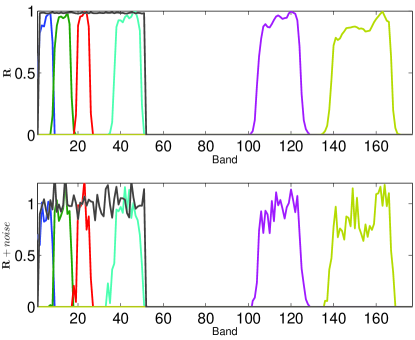
Figure 1: LANDSAT spectral responses. (Top) without noise. (Bottom) with an additive Gaussian noise with FSNR = 8dB.

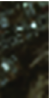
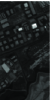
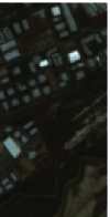
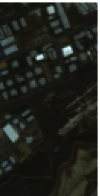
Figure 2: AVIRIS dataset: (Top left) HS Image. (Top middle) MS Image. (Top right) MAP [23]. (Bottom left) Wavelet MAP [24]. (Bottom middle) Hamiltonian MCMC. (Bottom right) Reference.

V-A1 Subspace learning

To learn the matrix $\mathbf{V}$ in (9), we propose to use the principal component analysis (PCA) which is a classical dimensionality reduction technique used in HS imagery. As in paragraph III-B1, the vectorized HS image ${\mathbf{z}}_{1}$ can be written as ${\mathbf{z}}_{1}=\left[{\boldsymbol{z}}_{1,1}^{T},{\boldsymbol{z}}_{1,2}^{T},\cdots,{\boldsymbol{z}}_{1,n_{\mathrm{x},1}n_{\mathrm{y},1}}^{T}\right]^{T}$, where ${\boldsymbol{z}}_{1,i}=\left[z_{1,i,1},z_{1,i,2},\cdots,z_{1,i,n_{\lambda,1}}\right]^{T}$. Then, the sample covariance matrix of the HS image ${\mathbf{z}}_{1}$ is diagonalized leading to

$$\mathbf{W}^{T}\boldsymbol{\Upsilon}\mathbf{W}=\mathbf{D}$$ (33)

where $\mathbf{W}$ is an $m_{\lambda}\times m_{\lambda}$ orthogonal matrix ($\mathbf{W}^{T}=\mathbf{W}^{-1}$) and $\mathbf{D}$ is a diagonal matrix whose diagonal elements are the ordered eigenvalues of $\boldsymbol{\Upsilon}$ denoted as $d_{1}\geq d_{2}\geq...\geq d_{m_{\lambda}}$. The dimension of the projection subspace $\widetilde{m}_{\lambda}$ is defined as the minimum integer satisfying the condition ${\sum_{i=1}^{\widetilde{m}_{\lambda}}d_{i}}/{\sum_{i=1}^{m_{\lambda}}d_{i}}\geq 0.99$. The matrix $\mathbf{V}$ is then constructed as the eigenvectors associated with the $\widetilde{m}_{\lambda}$ largest eigenvalues of $\boldsymbol{\Upsilon}$. As an illustration, the eigenvalues of the sample covariance matrix $\boldsymbol{\Upsilon}$ for the Moffett field image are displayed in Fig. 3. For this example, the $\widetilde{m}_{\lambda}=10$ eigenvectors contain $99.93\%$ of the information.

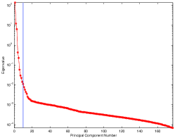
Figure 3: Eigenvalues of $\boldsymbol{\Upsilon}$ for the HS image.

V-A2 Hyper-hyperparameters selection

In our experiments, fixed hyper-hyperparameters have been chosen as follows: $\mathbf{\Psi}=\textbf{I}_{\widetilde{m}_{\lambda}},\eta=\widetilde{m}_{\lambda}+3.$

These choices can be motivated by the following arguments:

• The identity matrix assigned to $\mathbf{\Psi}$ ensures a non-informative prior.

• Setting the inverse gamma parameters to $\eta=\widetilde{m}_{\lambda}+3$ also leads to a non-informative prior [48].

• Note that parameter $\nu$ disappears when the joint posterior is integrated out with respect to parameter $\gamma$.

V-B Stepsize and Leapfrog Steps

The performance of the HMC method is mainly governed by the stepsize $\varepsilon$ and the number of leapfrog steps $N_{\textrm{L}}$. As pointed out in [34], a too large stepsize will result in a very low acceptance rate and a too small stepsize yields high computational complexity. In order to adjust the stepsize parameter $\varepsilon$, we propose to monitor the statistical acceptance ratio $\hat{\rho}_{t}$ defined as $\hat{\rho}_{t}=\frac{N_{\textrm{a,t}}}{N_{\textrm{W}}}$ where $N_{\textrm{W}}$ is the length of the counting window (in our experiment, the counting window at time $t$ contains the vectors $\tilde{{\mathbf{x}}}^{\left(t-N_{\textrm{W}}+1\right)},\tilde{{\mathbf{x}}}^{\left(t-N_{\textrm{W}}\right)},\cdots,\tilde{{\mathbf{x}}}^{\left(t\right)}$ with $N_{\textrm{W}}=50$) and $N_{\textrm{a,t}}$ is the number of accepted samples in this window at time $t$. As explained in [57], the adaptive tuning should adapt less and less as the algorithm proceeds to guarantee that the generated samples form a stationary Markov chain. In the proposed implementation, the parameter $\varepsilon$ is adjusted as in Algo. LABEL:algo:stepsize. The thresholds have been fixed to $(\alpha_{d},\alpha_{u})=(0.3,0.9)$ and the scale parameters are $(\beta_{d},\beta_{u})=(1.1,0.9)$ (these parameters were adjusted by cross-validation). Note that the initial value of $\varepsilon$ should not be too large to ‘blow up’ the leapfrog trajectory [34]. Generally, the stepsize converges after some iterations of Algo. LABEL:algo:stepsize.

    Algorithm 3:
Adjusting Stepsize

Regarding the number of leapfrogs, setting the trajectory length $N_{\textrm{L}}$ by trial and error is necessary [34]. To avoid the potential resonance, $N_{\textrm{L}}$ is randomly chosen from a uniform distribution from $N_{\textrm{min}}$ to $N_{\textrm{max}}$. After some preliminary runs and tests, $N_{\textrm{min}}=50$ and $N_{\textrm{max}}=55$ have been selected.

V-C Evaluation of the Fusion Quality

To evaluate the quality of the proposed fusion strategy, different image quality measures can be investigated. Referring to [24], we propose to use RSNR, SAM, UIQI, ERGAS and DD as defined below.

RSNR

The reconstruction SNR (RSNR) is related to the difference between the actual and fused images

$$\textrm{RSNR}({\mathbf{x}},\hat{{\mathbf{x}}})=10\log_{10}\left(\frac{\|{\mathbf{x}}\|^{2}}{\|{\mathbf{x}}-\hat{{\mathbf{x}}}\|_{2}^{2}}\right).$$ (34)

The larger RSNR, the better the fusion quality and vice versa.

SAM

The spectral angle mapper (SAM) measures the spectral distortion between the actual and estimated images. The SAM of two spectral vectors ${\boldsymbol{x}}_{n}$ and $\hat{{\boldsymbol{x}}}_{n}$ is defined as

$$\textrm{SAM}({\boldsymbol{x}}_{n},\hat{{\boldsymbol{x}}}_{n})=\textrm{arccos}\left(\frac{\langle{\boldsymbol{x}}_{n},\hat{{\boldsymbol{x}}}_{n}\rangle}{\|{\boldsymbol{x}}_{n}\|_{2}\|\hat{{\boldsymbol{x}}}_{n}\|_{2}}\right).$$ (35)

The average SAM is finally obtained by averaging the SAMs of all image pixels. Note that SAM value is expressed in radians and thus belongs to $[-\frac{\pi}{2},\frac{\pi}{2}]$. The smaller the absolute value of SAM, the less important the spectral distortion.

UIQI

The universal image quality index (UIQI) was proposed in [58] for evaluating the similarity between two single band images. It is related to the correlation, luminance distortion and contrast distortion of the estimated image to the reference image. The UIQI between ${\mathbf{a}}=[a_{1},a_{2},\cdots,a_{N}]$ and $\hat{{\mathbf{a}}}=[\hat{a}_{1},\hat{a}_{2},\cdots,\hat{a}_{N}]$ is defined as

$$\textrm{UIQI}({\mathbf{a}},\hat{{\mathbf{a}}})=\frac{4\sigma_{a\hat{a}}^{2}\mu_{a}\mu_{\hat{a}}}{(\sigma_{a}^{2}+\sigma_{\hat{a}}^{2})(\mu_{a}^{2}+\mu_{\hat{a}}^{2})}$$ (36)

where $\left(\mu_{a},\mu_{\hat{a}},\sigma_{a}^{2},\sigma_{\hat{a}}^{2}\right)$ are the sample means and variances of $a$ and $\hat{a}$, and $\sigma_{a\hat{a}}^{2}$ is the sample covariance of $\left(a,\hat{a}\right)$. The range of UIQI is $[-1,1]$ and UIQI$=1$ when ${\mathbf{a}}=\hat{{\mathbf{a}}}$. For multi-band image, the UIQI is obtained band-by-band and averaged over all bands.

ERGAS

The relative dimensionless global error in synthesis (ERGAS) calculates the amount of spectral distortion in the image [59]. This measure of fusion quality is defined as

$$\textrm{ERGAS}=100\times\frac{1}{d^{2}}\sqrt{\frac{1}{m_{\lambda}}\sum_{i=1}^{m_{\lambda}}\left(\frac{\textrm{RMSE}(i)}{\mu_{i}}\right)}$$ (37)

where $1/d^{2}$ is the ratio between the pixel sizes of the MS and HS images, $\mu_{i}$ is the mean of the $i$th band of the HS image, and $m_{\lambda}$ is the number of HS bands. The smaller ERGAS, the smaller the spectral distortion.

DD

The degree of distortion (DD) between two images ${\mathbf{X}}$ and $\hat{{\mathbf{X}}}$ is defined as

$$\textrm{DD}({\mathbf{X}},\hat{{\mathbf{X}}})=\frac{1}{M}\|\textrm{vec}({\mathbf{X}})-\textrm{vec}(\hat{{\mathbf{X}}})\|_{1}.$$ (38)

The smaller DD, the better the fusion.

V-D Comparison with other Bayesian models

The Bayesian model proposed here differs from previous Bayesian models [23, 24] in three-fold. First, in addition to the target image ${\mathbf{x}}$, the hierarchical Bayesian model allows the distributions of the noise variances ${\boldsymbol{s}}^{2}$ and the hyperparameter $\boldsymbol{\Sigma}_{{\boldsymbol{u}}}$ to be inferred. The hierarchical inference structure makes this Bayesian model more general and flexible. Second, the covariance matrix $\boldsymbol{\Sigma}_{{\boldsymbol{u}}}$ is assumed to be block diagonal, which allows us to exploit the correlations between spectral bands. Third, the proposed method takes advantage of the relation between the multispectral image and the target image by introducing a forward model ${\mathbf{F}}_{2}$. This paragraph compares the proposed Bayesian fusion method with these two state-of-the-art fusion algorithms [23] [24] for HS+MS fusion. The MMSE estimator of the image using the proposed Bayesian method is obtained from (22). In this simulation, $N_{\textrm{MC}}=500$ and $N_{\textrm{bi}}=500$. The fusion results obtained with different algorithms are depicted in Fig. 2. Graphically, the proposed algorithm performs competitively with the state-of-the-art methods. This result is confirmed quantitatively in Table II which shows the RSNR, UIQI, SAM, ERGAS and DD for the three methods. It can be seen that the HMC method provides slightly better results in terms of image restoration than the other methods. However, the proposed method allows the image covariance matrix and the noise variances to be estimated. The samples generated by the MCMC method can also be used to compute confidence intervals for the estimators (e.g., see error bars in Fig. 4).

TABLE II: Performance of different fusion methods in terms of: RSNR (db), UIQI, SAM (deg), ERGAS and DD($\times 10^{-2}$) (AVIRIS dataset).

Methods	RSNR	UIQI	SAM	ERGAS	DD	Time
MAP	23.33	0.9913	5.05	4.21	4.87	$\boldsymbol{1.6}$
Wavelet	25.53	0.9956	3.98	3.95	3.89	31
Proposed	$\boldsymbol{26.74}$	$\boldsymbol{0.9966}$	$\boldsymbol{3.40}$	$\boldsymbol{3.77}$	$\boldsymbol{3.33}$	530

V-E Estimation of the noise variances

The proposed Bayesian method allows noise variances ${s^{2}_{p,i}}$ $(i=1,\cdots,n_{\lambda,p},p=1,\cdots,P)$ to be estimated from the samples generated by the Gibbs sampler. The MMSE estimators of ${s^{2}_{1,(\cdot)}}$ and ${s^{2}_{2,(\cdot)}}$ are illustrated in Fig. 4. Graphically, the estimations can track the variations of the noise powers within tolerable discrepancy.

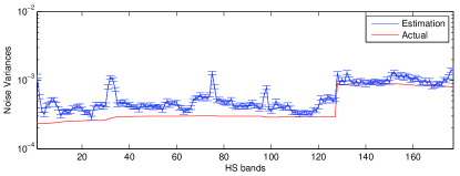
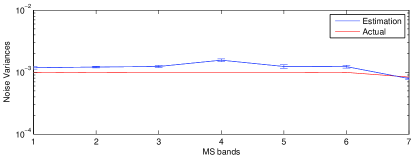
Figure 4: Noise variances and their MMSE estimates. (Top) HS image. (Bottom) MS image.

V-F Robustness with respect to the knowledge of ${\mathbf{F}}_{2}$

The sampling algorithm summarized in Algo. (LABEL:algo:HMC) requires the knowledge of the spectral response ${\mathbf{F}}_{2}$. However, this knowledge can be partially known in some practical applications. As the spectral response is the same for each vector ${\boldsymbol{x}}_{i}$ $(i=1,\cdots,m_{\mathrm{x}}m_{\mathrm{y}})$, ${\mathbf{F}}_{2}$ can be constructed from the matrix $f_{2}$ of size $n_{\lambda,2}\times m_{\lambda}$ (i.e., $7\times 172$) as follows

$${\mathbf{F}}_{2}=\textrm{diag}[\underbrace{f_{2}\cdots f_{2}}_{m_{\mathrm{x}}m_{\mathrm{y}}}].$$ (39)

This paragraph is devoted to testing the robustness of the proposed algorithm to the imperfect knowledge of $f_{2}$. In order to analyze this robustness, a zero-mean white Gaussian error has been added to any non-zero component of $f_{2}$ as shown in the bottom of Fig. 1. Of course, the level of uncertainty regarding $f_{2}$ is controlled by the variance of the error denoted as $\sigma_{2}^{2}$. The corresponding FSNR is defined to adjust the knowledge of $f_{2}$:

$$\textrm{FSNR}=10\log_{10}\left(\frac{\|f_{2}\|_{F}^{2}}{m_{\lambda}n_{\lambda,2}{s^{2}_{2}}}\right).$$ (40)

The larger FSNR, the more knowledge we have about $f_{2}$. The RSNRs between the reference and estimated images are displayed in Fig. 5 as a function of FSNR. Obviously, the performance of the proposed Bayesian fusion algorithm decreases as the uncertainty about $f_{2}$ increases. However, as long as the FSNR is above $8$dB, the performance of the proposed method always outperforms the MAP and wavelet-based MAP methods. Thus, the proposed method is quite robust with respect to the imperfect knowledge of $f_{2}$.

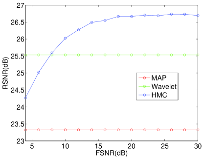
Figure 5: Reconstruction errors of the different fusion methods versus FSNR.

V-G Test on additional dataset

This section considers another reference image (the high spatial and high spectral image is a $128\times 64\times 93$ HS image with very high spatial resolution of 1.3 m/pixel) acquired by the Reflective Optics System Imaging Spectrometer (ROSIS) optical sensor over the urban area of the University of Pavia, Italy. The flight was operated by the Deutsches Zentrum für Luft- und Raumfahrt (DLR, the German Aerospace Agency) in the framework of the HySens project, managed and sponsored by the European Union. This image was initially composed of $115$ bands that have been reduced to $93$ bands after removing the water vapor absorption bands (with spectral range from 0.43 to 0.86 $\mu$m). This image has received a lot of attention in the remote sensing literature [60, 61, 62]. The HS blurring kernel is the same as in paragraph V-A and the MS spectral response is a $4$-band IKONOS-like reflectance spectral response. The noise level is defined by SNR${}_{1,\cdot}=35$dB for the first 43 bands and SNR${}_{1,\cdot}=30$dB for the remaining 50 bands of the HS image. For MS image, SNR_2,⋅ is 30dB for all bands. The ground-truth, HS, MS and fusion results obtained with different algorithms are displayed in Fig. 6. The corresponding image quality measures are reported in Table III. The estimates of the noise variances are shown in Fig. 7. These results are in good agreement with the performance obtained before.

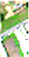
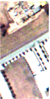
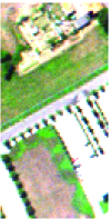
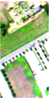
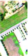
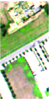
Figure 6: ROSIS dataset: (Top left) HS Image. (Top middle) MS Image. (Top right) MAP [23]. (Bottom left) Wavelet MAP [24]. (Bottom middle) Hamiltonian MCMC. (Bottom right) Reference.

TABLE III: Performance of different fusion methods in terms of: RSNR (db), UIQI, SAM (deg), ERGAS and DD($\times 10^{-2}$) (ROSIS dataset).

Methods	RSNR	UIQI	SAM	ERGAS	DD	Time(s)
MAP [23]	26.58	0.9926	2.90	1.36	3.61	$\boldsymbol{1.5}$
Wavelet [24]	26.62	0.9925	2.87	1.35	3.60	30
Proposed	$\boldsymbol{27.30}$	$\boldsymbol{0.9933}$	$\boldsymbol{2.60}$	$\boldsymbol{1.24}$	$\boldsymbol{3.27}$	410

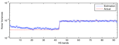
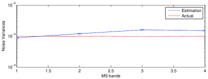
Figure 7: Noise variances and their MMSE estimates (ROSIS dataset). (Top) HS image. (Bottom) MS image.

V-H Application to pansharpening

The proposed algorithm can also be used for pansharpening, which is a quite important and popular application in the area of remote sensing. In this section, we focus on fusing panchromatic and hyperspectral images (HS+PAN), which is the extension of conventional pansharpening (MS+PAN). The HS image considered in this section was used in paragraph V-G whereas the PAN image was obtained by averaging all the high resolution HS bands. The SNR of the PAN image is $30$dB. Apart from [23, 24], we also compare the results with the method of [63], which proposes a popular pansharpening method. The results are displayed in Fig. 8 and the quantitative results are reported in Table IV. The proposed Bayesian method still provides interesting results.

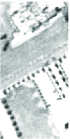
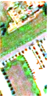
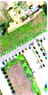
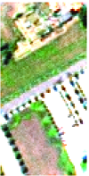
Figure 8: ROSIS dataset: (Top left) Reference. (Top middle) MS Image. (Top right) Adaptive IHS [63]. (Bottom left) MAP [23]. (Bottom middle) Wavelet MAP [24]. (Bottom right) Hamiltonian MCMC.

TABLE IV: Performance of different fusion methods in terms of: RSNR (db), UIQI, SAM (deg), ERGAS and DD($\times 10^{-2}$) (ROSIS dataset).

Methods	RSNR	UIQI	SAM	ERGAS	DD	Time(s)
AIHS [63]	16.69	0.9176	7.23	4.24	9.99	7.7
MAP [23]	17.54	0.9177	6.55	3.78	8.78	$\boldsymbol{1.4}$
Wavelet [24]	18.03	0.9302	6.08	3.57	8.33	26
Proposed	$\boldsymbol{18.23}$	$\boldsymbol{0.9341}$	$\boldsymbol{6.05}$	$\boldsymbol{3.49}$	$\boldsymbol{8.20}$	387

VI Conclusions

This paper proposed a hierarchical Bayesian model to fuse multiple multi-band images with various spectral and spatial resolutions. The image to be recovered was assumed to be degraded according to physical transformations included within a forward model. An appropriate prior distribution, that exploited geometrical concepts encountered in spectral unmixing problems was proposed. The resulting posterior distribution was efficiently sampled thanks to a Hamiltonian Monte Carlo algorithm. Simulations conducted on pseudo-real data showed that the proposed method competed with the state-of-the-art techniques to fuse MS and HS images. These experiments also illustrated the robustness of the proposed method with respect to the misspecification of the forward model. Future work includes the estimation of the parameters involved in the forward model (e.g., the spatial and spectral responses of the sensors) to obtain a fully unsupervised fusion algorithm. The incorporation of spectral mixing constraints for a possible improved spectral accuracy for the estimated high resolution image would also deserve some attention.

References

- [1] I. Amro, J. Mateos, M. Vega, R. Molina, and A. K. Katsaggelos, “A survey of classical methods and new trends in pansharpening of multispectral images,” EURASIP J. Adv. Signal Process., vol. 2011, no. 1, pp. 1–22, 2011.
- [2] W. Dou, Y. Chen, X. Li, and D. Z. Sui, “A general framework for component substitution image fusion: An implementation using the fast image fusion method,” Comput. & Geosci., vol. 33, no. 2, pp. 219–228, 2007.
- [3] L. Wald, “Some terms of reference in data fusion,” IEEE Trans. Geosci. and Remote Sens., vol. 37, no. 3, pp. 1190 –1193, May 1999.
- [4] T.-M. Tu, P. S. Huang, C.-L. Hung, and C.-P. Chang, “A fast intensity-hue-saturation fusion technique with spectral adjustment for IKONOS imagery,” IEEE Geosci. and Remote Sensing Lett., vol. 1, no. 4, pp. 309–312, 2004.
- [5] H. Aanaes, J. Sveinsson, A. Nielsen, T. Bovith, and J. Benediktsson, “Model-based satellite image fusion,” IEEE Trans. Geosci. and Remote Sens., vol. 46, no. 5, pp. 1336–1346, May 2008.
- [6] M. Joshi and A. Jalobeanu, “MAP estimation for multiresolution fusion in remotely sensed images using an IGMRF prior model,” IEEE Trans. Geosci. and Remote Sens., vol. 48, no. 3, pp. 1245–1255, March 2010.
- [7] D. Liu and P. T. Boufounos, “Dictionary learning based pan-sharpening,” in Proc. IEEE Int. Conf. Acoust., Speech, and Signal Processing (ICASSP), Kyoto, Japan, March 2012, pp. 2397–2400.
- [8] D. Manolakis and G. Shaw, “Detection algorithms for hyperspectral imaging applications,” IEEE Signal Process. Mag., vol. 19, no. 1, pp. 29–43, jan 2002.
- [9] C.-I Chang, Hyperspectral Imaging: Techniques for Spectral detection and classification. New York: Kluwer, 2003.
- [10] J. M. Bioucas-Dias, A. Plaza, N. Dobigeon, M. Parente, Q. Du, P. Gader, and J. Chanussot, “Hyperspectral unmixing overview: Geometrical, statistical, and sparse regression-based approaches,” IEEE J. Sel. Topics Appl. Earth Observations and Remote Sens., vol. 5, no. 2, pp. 354–379, 2012.
- [11] M. Cetin and N. Musaoglu, “Merging hyperspectral and panchromatic image data: qualitative and quantitative analysis,” Int. J. Remote Sens., vol. 30, no. 7, pp. 1779–1804, 2009.
- [12] G. A. Licciardi, M. M. Khan, J. Chanussot, A. Montanvert, L. Condat, and C. Jutten, “Fusion of hyperspectral and panchromatic images using multiresolution analysis and nonlinear pca band reduction,” EURASIP J. Adv. Signal Process., vol. 2012, no. 1, pp. 1–17, 2012.
- [13] M. Moeller, T. Wittman, and A. L. Bertozzi, “A variational approach to hyperspectral image fusion,” in Proc. SPIE Defense, Security, and Sensing. International Society for Optics and Photonics, 2009, pp. 73 341E–73 341E.
- [14] C. Chisense, J. Engels, M. Hahn, and E. Gülch, “Pansharpening of hyperspectral images in urban areas,” in Proc. XXII Congr. of the Int. Society for Photogrammetry, Remote Sens., Melbourne, Australia, 2012.
- [15] M. E. Winter and E. Winter, “Resolution enhancement of hyperspectral data,” in Proc. IEEE Aerospace Conference, 2002, pp. 3–1523.
- [16] G. Chen, S.-E. Qian, J.-P. Ardouin, and W. Xie, “Super-resolution of hyperspectral imagery using complex ridgelet transform,” Int. J. Wavelets, Multiresolution Inf. Process., vol. 10, no. 03, 2012.
- [17] D. Inc., “Worldview-3,” http://www.satimagingcorp.com/satellite-sensors/WorldView3-DS-WV3-Web.pdf, Jan. 2013.
- [18] N. Ohgi, A. Iwasaki, T. Kawashima, and H. Inada, “Japanese hyper-multi spectral mission,” in Proc. IEEE Int. Conf. Geosci. Remote Sens. (IGARSS), Honolulu, Hawaii, USA, July 2010, pp. 3756–3759.
- [19] N. Yokoya and A. Iwasaki, “Hyperspectral and multispectral data fusion mission on hyperspectral imager suite (HISUI),” in Proc. IEEE Int. Conf. Geosci. Remote Sens. (IGARSS), Melbourne, Australia, July 2013, pp. 4086–4089.
- [20] V. Shettigara, “A generalized component substitution technique for spatial enhancement of multispectral images using a higher resolution data set,” Photogramm. Eng. Remote Sens., vol. 58, no. 5, pp. 561–567, 1992.
- [21] J. Zhou, D. Civco, and J. Silander, “A wavelet transform method to merge Landsat TM and SPOT panchromatic data,” Int. J. Remote Sens., vol. 19, no. 4, pp. 743–757, 1998.
- [22] M. González-Audícana, J. L. Saleta, R. G. Catalán, and R. García, “Fusion of multispectral and panchromatic images using improved IHS and PCA mergers based on wavelet decomposition,” IEEE Trans. Geosci. and Remote Sens., vol. 42, no. 6, pp. 1291–1299, 2004.
- [23] R. C. Hardie, M. T. Eismann, and G. L. Wilson, “MAP estimation for hyperspectral image resolution enhancement using an auxiliary sensor,” IEEE Trans. Image Process., vol. 13, no. 9, pp. 1174–1184, Sept. 2004.
- [24] Y. Zhang, S. De Backer, and P. Scheunders, “Noise-resistant wavelet-based Bayesian fusion of multispectral and hyperspectral images,” IEEE Trans. Geosci. and Remote Sens., vol. 47, no. 11, pp. 3834 –3843, Nov. 2009.
- [25] Y. Zhang, A. Duijster, and P. Scheunders, “A Bayesian restoration approach for hyperspectral images,” IEEE Trans. Geosci. and Remote Sens., vol. 50, no. 9, pp. 3453 –3462, Sep. 2012.
- [26] M. T. Eismann and R. C. Hardie, “Application of the stochastic mixing model to hyperspectral resolution enhancement,” IEEE Trans. Geosci. and Remote Sens., vol. 42, no. 9, pp. 1924–1933, Sept. 2004.
- [27] ——, “Hyperspectral resolution enhancement using high-resolution multispectral imagery with arbitrary response functions,” IEEE Trans. Image Process., vol. 43, no. 3, pp. 455–465, March 2005.
- [28] X. Otazu, M. Gonzalez-Audicana, O. Fors, and J. Nunez, “Introduction of sensor spectral response into image fusion methods. Application to wavelet-based methods,” IEEE Trans. Geosci. and Remote Sens., vol. 43, no. 10, pp. 2376–2385, 2005.
- [29] M. V. Joshi, L. Bruzzone, and S. Chaudhuri, “A model-based approach to multiresolution fusion in remotely sensed images,” IEEE Trans. Geosci. and Remote Sens., vol. 44, no. 9, pp. 2549–2562, Sept. 2006.
- [30] G. Casella and E. I. George, “Explaining the Gibbs sampler,” The American Statistician, vol. 46, no. 3, pp. 167–174, 1992.
- [31] W. K. Hastings, “Monte Carlo sampling methods using Markov chains and their applications,” Biometrika, vol. 57, no. 1, pp. 97–109, 1970.
- [32] S. Duane, A. D. Kennedy, B. J. Pendleton, and D. Roweth, “Hybrid Monte Carlo,” Physics Lett. B, vol. 195, no. 2, pp. 216–222, Sept. 1987.
- [33] R. M. Neal, “Probabilistic inference using Markov chain Monte Carlo methods,” Dept. of Computer Science, University of Toronto, Tech. Rep. CRG-TR-93-1, Sept. 1993.
- [34] ——, “MCMC using Hamiltonian dynamics,” Handbook of Markov Chain Monte Carlo, vol. 54, pp. 113–162, 2010.
- [35] D. Fasbender, D. Tuia, P. Bogaert, and M. Kanevski, “Support-based implementation of Bayesian data fusion for spatial enhancement: Applications to ASTER thermal images,” IEEE Geosci. and Remote Sensing Lett., vol. 5, no. 4, pp. 598–602, Oct. 2008.
- [36] M. Elbakary and M. Alam, “Superresolution construction of multispectral imagery based on local enhancement,” IEEE Geosci. and Remote Sensing Lett., vol. 5, no. 2, pp. 276–279, April 2008.
- [37] J. B. Campbell, Introduction to remote sensing, 3rd ed. New-York, NY: Taylor & Francis, 2002.
- [38] A. Jalobeanu, L. Blanc-Feraud, and J. Zerubia, “An adaptive Gaussian model for satellite image deblurring,” IEEE Trans. Image Process., vol. 13, no. 4, pp. 613–621, 2004.
- [39] A. Duijster, P. Scheunders, and S. De Backer, “Wavelet-based em algorithm for multispectral-image restoration,” IEEE Trans. Geosci. and Remote Sens., vol. 47, no. 11, pp. 3892–3898, 2009.
- [40] M. Xu, H. Chen, and P. K. Varshney, “An image fusion approach based on Markov random fields,” IEEE Trans. Geosci. and Remote Sens., vol. 49, no. 12, pp. 5116–5127, 2011.
- [41] N. Dobigeon, J.-Y. Tourneret, and A. O. Hero III, “Bayesian linear unmixing of hyperspectral images corrupted by colored Gaussian noise with unknown covariance matrix,” in Proc. IEEE Int. Conf. Acoust., Speech, and Signal Processing (ICASSP), Las Vegas, USA, March 2008, pp. 3433–3436.
- [42] R. Schultz and R. Stevenson, “A Bayesian approach to image expansion for improved definition,” IEEE Trans. Image Process., vol. 3, no. 3, pp. 233–242, May 1994.
- [43] C.-I. Chang, X.-L. Zhao, M. L. Althouse, and J. J. Pan, “Least squares subspace projection approach to mixed pixel classification for hyperspectral images,” IEEE Trans. Geosci. and Remote Sens., vol. 36, no. 3, pp. 898–912, 1998.
- [44] J. M. Bioucas-Dias and J. M. Nascimento, “Hyperspectral subspace identification,” IEEE Trans. Geosci. and Remote Sens., vol. 46, no. 8, pp. 2435–2445, 2008.
- [45] R. C. Hardie, K. J. Barnard, and E. E. Armstrong, “Joint MAP registration and high-resolution image estimation using a sequence of undersampled images,” IEEE Trans. Image Process., vol. 6, no. 12, pp. 1621–1633, Dec. 1997.
- [46] N. A. Woods, N. P. Galatsanos, and A. K. Katsaggelos, “Stochastic methods for joint registration, restoration, and interpolation of multiple undersampled images,” IEEE Trans. Image Process., vol. 15, no. 1, pp. 201–213, Jan. 2006.
- [47] Q. Wei, N. Dobigeon, and J.-Y. Tourneret, “Bayesian fusion of multi-band images,” IRIT-ENSEEIHT, Tech. Report, Univ. of Toulouse, 2014. [Online]. Available: http://wei.perso.enseeiht.fr/papers/2014QiTechnicalReport.pdf
- [48] E. Punskaya, C. Andrieu, A. Doucet, and W. Fitzgerald, “Bayesian curve fitting using MCMC with applications to signal segmentation,” IEEE Trans. Signal Process., vol. 50, no. 3, pp. 747–758, March 2002.
- [49] A. Gelman, “Prior distributions for variance parameters in hierarchical models (comment on article by browne and draper),” Bayesian analysis, vol. 1, no. 3, pp. 515–534, 2006.
- [50] C. P. Robert, The Bayesian Choice: from Decision-Theoretic Motivations to Computational Implementation, 2nd ed., ser. Springer Texts in Statistics. New York, NY, USA: Springer-Verlag, 2007.
- [51] S. Bidon, O. Besson, and J.-Y. Tourneret, “The adaptive coherence estimator is the generalized likelihood ratio test for a class of heterogeneous environments,” IEEE Signal Process. Lett., vol. 15, pp. 281–284, 2008.
- [52] M. Bouriga and O. Féron, “Estimation of covariance matrices based on hierarchical inverse-Wishart priors,” J. of Stat. Planning and Inference, 2012.
- [53] H. Zhang, Y. Zhang, H. Li, and T. S. Huang, “Generative Bayesian image super resolution with natural image prior,” IEEE Trans. Image Process., vol. 21, no. 9, pp. 4054–4067, 2012.
- [54] F. Orieux, O. Féron, and J.-F. Giovannelli, “Sampling high-dimensional Gaussian distributions for general linear inverse problems,” IEEE Signal Process. Lett., vol. 19, no. 5, pp. 251–254, 2012.
- [55] D. Ceperley, Y. Chen, R. V. Craiu, X.-L. Meng, A. Mira, and J. Rosenthal, “Challenges and advances in high dimensional and high complexity monte carlo computation and theory,” in Banff International Research Station, 2012.
- [56] R. O. Green, M. L. Eastwood, C. M. Sarture, T. G. Chrien, M. Aronsson, B. J. Chippendale, J. A. Faust, B. E. Pavri, C. J. Chovit, M. Solis et al., “Imaging spectroscopy and the airborne visible/infrared imaging spectrometer (AVIRIS),” Remote Sens. of Environment, vol. 65, no. 3, pp. 227–248, 1998.
- [57] G. O. Roberts and J. S. Rosenthal, “Coupling and ergodicity of adaptive Markov Chain Monte Carlo algorithms,” J. of Appl. Probability, vol. 44, no. 2, pp. pp. 458–475, 2007. [Online]. Available: http://www.jstor.org/stable/27595854
- [58] Z. Wang and A. C. Bovik, “A universal image quality index,” IEEE Signal Process. Lett., vol. 9, no. 3, pp. 81–84, 2002.
- [59] L. Wald, “Quality of high resolution synthesised images: Is there a simple criterion?” in Proc. Int. Conf. Fusion of Earth Data, Nice, France, Jan 2000, pp. 99–103.
- [60] A. Plaza, J. A. Benediktsson, J. W. Boardman, J. Brazile, L. Bruzzone, G. Camps-Valls, J. Chanussot, M. Fauvel, P. Gamba, A. Gualtieri, M. Marconcini, J. C. Tilton, and G. Trianni, “Recent advances in techniques for hyperspectral image processing,” Remote Sensing of Environment, vol. 113, Supplement 1, pp. S110–S122, 2009.
- [61] Y. Tarabalka, M. Fauvel, J. Chanussot, and J. Benediktsson, “SVM- and MRF-based method for accurate classification of hyperspectral images,” IEEE Trans. Geosci. and Remote Sens., vol. 7, no. 4, pp. 736–740, 2010.
- [62] J. Li, J. M. Bioucas-Dias, and A. Plaza, “Spectral-spatial classification of hyperspectral data using loopy belief propagation and active learning,” IEEE Trans. Geosci. and Remote Sens., vol. 51, no. 2, pp. 844–856, 2013.
- [63] S. Rahmani, M. Strait, D. Merkurjev, M. Moeller, and T. Wittman, “An adaptive IHS pan-sharpening method,” IEEE Geosci. and Remote Sensing Lett., vol. 7, no. 4, pp. 746–750, 2010.