Sparse additive regression on a regular lattice

Abstract

We consider estimation in a sparse additive regression model with the design points on a regular lattice. We establish the minimax convergence rates over Sobolev classes and propose a Fourier-based rate-optimal estimator which is adaptive to the unknown sparsity and smoothness of the response function. The estimator is derived within Bayesian formalism but can be naturally viewed as a penalized maximum likelihood estimator with the complexity penalties on the number of nonzero univariate additive components of the response and on the numbers of the nonzero coefficients of their Fourer expansions. We compare it with several existing counterparts and perform a short simulation study to demonstrate its performance.

Keywords: Adaptive minimaxity; additive models; complexity penalty; maximum a posteriori rule; sparsity.

1 Introduction

Consider a general nonparametric $d$-dimensional regression model, where the design points are located on a regular lattice of size $n_{1}\times\ldots\times n_{d}$ on $[0,1]^{d}$:

$$y(i_{1}/n_{1},\ldots,i_{d}/n_{d})=f(i_{1}/n_{1},\ldots,i_{d}/n_{d})+\epsilon(i_{1}/n_{1},...,i_{d}/n_{d}),\quad i_{j}=0,\ldots,n_{j}-1;\;j=1,\ldots d$$ (1)

$\epsilon(i_{1}/n_{1},...,i_{d}/n_{d})\sim{\cal N}(0,\sigma^{2})$ and are independent, and the unknown response function $f:\mathbb{R}^{d}\rightarrow\mathbb{R}$ is assumed to belong to a class of functions of certain smoothness. Let $N=\prod_{j=1}^{d}n_{j}$ be the overall number of observations in the model (1).

In particular, a regular grid can be useful for design of experiments when one has some prior belief on the relative relevance of predictors. Thus, he can use a finer grid (larger $n_{j}$) for more important variables and a coarse grid (smaller $n_{j}$) otherwise.

When $d$ is large, estimation of $f$ in (1) suffers severely from “curse of dimensionality” problem. A typical remedy is to impose some addition structural constraints on $f$. One of the common approaches is to consider the class of additive models (Hastie & Tibshirani, 1990), where the unknown $f$ can be decomposed in a sum of $d$ univariate functions: $f(x_{1},\ldots,x_{d})=\sum_{j=1}^{d}f_{j}(x_{j})$. The original model (1) becomes then

$$y(i_{1}/n_{1},\ldots,i_{d}/n_{d})=a_{0}+\sum_{j=1}^{d}f_{j}(i_{j}/n_{j})+\epsilon(i_{1}/n_{1},...,i_{d}/n_{d}),\quad i_{j}=0,\ldots,n_{j}-1;\;j=1,\ldots d.$$ (2)

To make the model (2) identifiable, we impose $\sum_{i=0}^{n_{j}-1}f_{j}(i/n_{j})=0$ for all $j=1,\ldots,d$. The goal is to estimate the unknown global mean $a_{0}$ and the functions $f_{j}$’s.

Additive models have become a standard tool in multivariate nonparametric regression and can be efficiently fitted by the backfitting algorithm of Friedman & Stuetzle (1981). However, in a variety of modern high-dimensional statistical setups the number of predictors $d$ may be still large relatively to the amount of observed data. A key extra assumption then is sparsity, where it is assumed that only a small fraction of $f_{j}$ in (2) has a truly relevant impact on the response while other $f_{j}=0$. Let ${\cal J}_{0}$ and ${\cal J}_{0}^{c}$ be the (unknown) subsets of indices corresponding respectively to the zero and nonzero $f_{j}$. The sparse additive model is

$$y(i_{1}/n_{1},\ldots,i_{d}/n_{d})=a_{0}+\sum_{j\in{\cal J}_{0}^{c}}f_{j}(i_{j}/n_{j})+\epsilon(i_{1}/n_{1},...,i_{d}/n_{d}),\quad i_{j}=0,\ldots,n_{j}-1;\;j=1,\ldots d$$ (3)

and $\sum_{i=0}^{n_{j}-1}f_{j}(i/n_{j})=0,\;j\in{\cal J}_{0}^{c}$.

Expand each $f_{j},\;j\in{\cal J}_{0}^{c}$ in the orthogonal discrete Fourier series assuming for simplicity of exposition that all $n_{j}$ are odd:

$$f_{j}(i/n_{j})=\sum_{k=-(n_{j}-1)/2}^{(n_{j}-1)/2}c_{kj}e^{-\frac{2\pi Iki}{n_{j}}},$$

where $I=\sqrt{-1}$ and discrete Fourier coefficients

$$c_{kj}=\frac{1}{n_{j}}\sum_{i=0}^{n_{j}-1}f_{j}(i/n_{j})e^{\frac{2\pi Iki}{n_{j}}}.$$ (4)

The identifiability condition $\sum_{i=0}^{n_{j}-1}f_{j}(i/n_{j})=0$ implies $c_{0j}=0$.

One should make some assumptions on regularity properties of $f_{j}$. We assume that the vector of discrete Fourier coefficients $c_{j}$ of $f_{j}$ in (4) belongs to a Sobolev ellipsoid $\Theta_{n_{j}}(s_{j},R_{j})=\{c_{j}:\sum_{k=-(n_{j}-1)/2}^{(n_{j}-1)/2}|c_{kj}|^{2}|k|^{2s_{j}}\leq R^{2}_{j};\;c_{0j}=0\}$, where $s_{j}>1/2$ and $R_{j}<C_{R}$ for some constant $C_{R}>0$, and denote the corresponding class of functions $f_{j}$ by ${\cal F}_{n_{j}}(s_{j},R_{j})$. The class ${\cal F}_{n_{j}}(s_{j},R_{j})$ is a discrete analog of a Sobolev ball of functions of smoothness $s_{j}$ with a radius $R_{j}$ (see, e.g., Korostelev & Korosteleva, 2011, Section 10.5).

We establish the minimax rates of estimating $f$ in (3), where $f_{j}\in{\cal F}_{n_{j}}(s_{j},R_{j})$. The corresponding rates for the case of $N$ distinct points for each predictor $x_{j}$ were derived in Raskutti, Wainwright & Yu (2012). However, we consider a design on the regular lattice, where there are $N/n_{j}$ repeated observations at each of $n_{j}$ grid points for every $x_{j}$. It turns out that this difference affects the resulting minimax rates.

In particular, we show that the average mean squared error $AMSE(\hat{f}_{j},f_{j})=\frac{1}{n_{j}}E||\hat{f}_{j}-f_{j}||^{2}_{n_{j}}$ for estimating a single univariate function $f_{j}\in{\cal F}_{n_{j}}(s_{j},R_{j})$ in the model (3) at the design points, where a general notation $||\cdot||_{n}$ is used for Euclidean norm in $\mathbb{R}^{n}$, is of the order

$$\min\left(N^{-\frac{2s_{j}}{2s_{j}+1}},\frac{n_{j}}{N}\right).$$ (5)

For sufficiently smooth $f_{j}$ with $2s_{j}+1\geq\ln N/\ln n_{j}$, the rate in (5) is the standard minimax rate $N^{-2s_{j}/(2s_{j}+1)}$ for nonparametric estimation of a univariate function from ${\cal F}_{n_{j}}(s_{j},R_{j})$ (see, e.g., Korostelev & Korosteleva, 2011, Section 10.5), but for $2s_{j}+1<\ln N/\ln n_{j}$ it corresponds to the parametric rate of estimating $f_{j}$ at each grid point $i/n_{j}$ by simple averaging over the corresponding $N/n_{j}$ replications. To understand this phenomenon recall that in a standard nonparametric regression setup smoothing (local averaging over neighbour points) is necessary to reduce the variance. Although it introduces bias, the effect of the latter is negligible under smoothness assumptions on an unknown response function, while the benefits of variance reduction are essential. As we have mentioned above, in the considered case there are $N/n_{j}$ repeated observations at each grid point $i/n_{j}$ and the variance can already be reduced by their averaging without causing any bias. On the other hand, the grid might be too coarse to use neighbour points in smoothing since the resulting bias becomes dominating in the bias-variance tradeoff for nonsmooth $f_{j}$, where $2s_{j}+1<\ln N/\ln n_{j}$.

In particular, when all $n_{j}=N^{1/d}$ are equal, the minimax $AMSE(\hat{f}_{j},f_{j})$ in (5) is of the order $N^{-r_{j}}$, where $r_{j}=\max\left(\frac{2s_{j}}{2s_{j}+1},1-\frac{1}{d}\right)$ and the parametric rate of averaging occurs when $2s_{j}+1<d$.

Furthermore, we prove that the overall minimax $AMSE(\hat{f},f)=\frac{1}{N}E||\hat{f}-f||^{2}_{N}$ for the sparse additive models with $d_{0}=|{\cal J}_{0}^{c}|$ nonzero $f_{j}$ is of the order

$$\max\left(\sum_{j\in{\cal J}_{0}^{c}}\min\left(N^{-\frac{2s_{j}}{2s_{j}+1}},\frac{n_{j}}{N}\right),\frac{d_{0}\ln(d/d_{0})}{N}\right).$$ (6)

The term $\sum_{j\in{\cal J}_{0}^{c}}\min\left(N^{-\frac{2s_{j}}{2s_{j}+1}},\frac{n_{j}}{N}\right)$ in (6) is associated with the minimax rates of estimating $d_{0}$ nonzero univariate functions in ${\cal F}_{n_{j}}(s_{j},R_{j}),\;j\in{\cal J}_{0}^{c}$, while $\frac{d_{0}\ln(d/d_{0})}{N}$ corresponds to the error of selecting a subset of $d_{0}$ nonzero elements out of $d$ and appears in various related model selection setups (e.g., Abramovich & Grinshtein, 2010, 2013; Raskutti, Wainwright & Yu, 2011, 2012; Rigollet & Tsybakov, 2011). For the design with $N$ distinct points for each $x_{j}$, the similar rate $\max\left(\sum_{j\in{\cal J}_{0}^{c}}N^{-r_{j}},\frac{d_{0}\ln(d/d_{0})}{N}\right)$, where $r_{j}=2s_{j}/(2s_{j}+1)$, was derived in Raskutti, Wainright & Yu (2012).

We also propose a rate-optimal estimator for estimating sparse additive models (3) which is adaptive to the unknown parameters $(s_{j},R_{j}),\;j\in{\cal J}_{0}^{c}$ of Sobolev ellipsoids and to the unknown sparsity $d_{0}$. The estimation is performed in the Fourier domain and is based on identifying nonzero vectors of (univariate) discrete Fourier coefficients $c_{j}$ by imposing a penalty on the number of nonzero $c_{j}$’s and estimating their components by truncating the corresponding series of empirical Fourier coefficients of the data, and can be efficiently computed. The resulting estimator is developed within a Bayesian framework and can be viewed as a maximum a posteriori (MAP) sparse additive estimator. From a frequentist view, it corresponds to penalized maximum likelihood estimation of $c_{j}$ with the complexity type of penalties on the number of nonzero $c_{j}$ and numbers of their nonzero entries.

We compare the sparse additive MAP estimator with several existing counterparts proposed recently in the literature, e.g., COSSO of Lin & Zhang (2006), SPAM of Ravikumar et al. (2009), sparse additive estimator of Meier, van de Geer & Bühlmann (2009) and $M$-estimator of Raskutti, Wainwright & Yu (2012) (see also Koltchinskii & Yuan, 2010 and Suzuki & Sugiyama, 2013). In the Fourier domain, the above estimators also correspond to penalized maximum likelihood estimation of $c_{j}$ but with penalties on the magnitudes of $c_{kj}$ rather than on their cardinality. However, only the $M$-estimator is proved to be rate-optimal (in the minimax sense) for the case when there are $N$ distinct observations for each predictor $x_{j}$. Moreover, all those procedures (except SPAM) are not adaptive to the smoothness $s_{j}$ of $f_{j}$.

The paper is organized as follows. In Section 2 we derive the sparse additive MAP estimator. Its asymptotic adaptive minimaxity is established in Section 3, where we compare it also with its existing counterparts. The results of a simulation study are given in Section 4. Some concluding remarks and possible extensions are discussed in Section 5. All the proofs are placed in the Appendix.

2 MAP estimator

2.1 Main idea

For any fixed $j=1,\ldots,d$, averaging a general additive model (2) over all $N/n_{j}$ observations at points $i_{j}/n_{j}$ and using the identifiability conditions yields

$$\begin{split}\bar{y}_{j}(i_{j}/n_{j})=&\frac{n_{j}}{N}\sum_{i_{1}=0}^{n_{1}-1}\ldots\sum_{i_{j-1}=0}^{n_{j-1}-1}\sum_{i_{j+1}=0}^{n_{j+1}-1}\ldots\sum_{i_{d}=0}^{n_{d}-1}y(i_{1}/n_{1},\ldots,i_{j}/n_{j},\ldots,i_{d}/n_{d})\\ =&a_{0}+f_{j}(i_{j}/n_{j})+\epsilon^{\prime}(i_{j}/n_{j}),\quad i_{j}=0,\ldots,n_{j}\end{split}$$ (7)

where $\epsilon^{\prime}(i/n_{j})\sim{\cal N}(0,\frac{n_{j}}{N}\sigma^{2})$ and are independent.

Equivalently, in the Fourier domain one has

$$\xi_{kj}=c_{kj}+\frac{\sigma^{2}}{N}z_{kj},\quad k=-(n_{j}-1)/2,\ldots,(n_{j}-1)/2;\;j=1,\ldots,d,$$ (8)

where

$$\xi_{kj}=\frac{1}{n_{j}}\sum_{i=0}^{n_{j}-1}\bar{y}_{j}(i/n_{j})e^{\frac{2\pi Iki}{n_{j}}}$$

are discrete (one-dimensional) Fourier coefficients of the vector $\bar{y}_{j}$, $c_{kj}$ are given in (4) and $z_{kj}$ are independent standard complex normal variates.

The goal now is to estimate the unknown discrete Fourier coefficients $c_{kj}$ in (8) by some $\hat{c}_{kj}$. The resulting estimator $\hat{f}$ in the original domain will then be

$$\hat{f}(i_{1}/n_{1},\ldots,i_{d}/n_{d})=\hat{a}_{0}+\sum_{j=1}^{d}\hat{f}_{j}(i_{j}/n_{j})=\hat{a}_{0}+\sum_{j=1}^{d}\sum_{k=-(n_{j}-1)/2}^{(n_{j}-1)/2}\hat{c}_{kj}e^{\frac{I2\pi ki_{j}}{n_{j}}}.$$

Additivity of $f$ and Parseval’s equality imply

$$AMSE(\hat{f},f)=E|\hat{a}_{0}-a_{0}|^{2}+\sum_{j=1}^{d}E||\hat{c}_{j}-c_{j}||^{2}_{n_{j}}$$

and the original dimensionality of the problem $N$ is thus reduced to $\sum_{j=1}^{d}(n_{j}-1)+1$ in the Fourier domain (recall that $c_{0j}=0$ for all $j$).

Estimate the overall mean $a_{0}$ by the overall sample mean $\bar{y}$. Due the identifiability conditions $\sum_{i=0}^{n-1}f_{j}(i/n)=0$, we have

$$\bar{y}=a_{0}+\epsilon^{*},$$

where $\epsilon^{*}\sim{\cal N}(0,\frac{\sigma^{2}}{N})$, yielding $E|\bar{y}-a_{0}|^{2}=\frac{\sigma^{2}}{N}$. Furthermore, we naturally set $\hat{c}_{0j}=0$ for all $j$ with no error and, therefore, $\sum_{i=0}^{n_{j}-1}\hat{f}_{j}(i/n_{j})=0$.

Recall now that we consider a sparse additive model (3), where most $f_{j}$ and, therefore, $c_{j}$ are zeros. Under the assumption $f_{j}\in{\cal F}_{n_{j}}(s_{j},R_{j}),\;j\in{\cal J}_{0}^{c}$, the corresponding $c_{kj}$ decrease polynomially in $k$ and $c_{j}$ can be well-approximated by several first $c_{kj}$. The proposed algorithm tries first to identify the set ${\cal J}_{0}^{c}$ of nonzero vectors $c_{j}$ and then estimates their entries by truncating the corresponding vectors $\xi_{j}$ of empirical discrete Fourier coefficients in (8) at the properly adaptively chosen cut-points.

2.2 Derivation

For nonzero vectors $c_{j}$ in (8) we consider truncated estimators of the form $\hat{c}_{kj}=\xi_{kj},\;|k|=1,\ldots,k_{j}$ and zero otherwise. Thus, if we knew the set of indices ${\cal J}_{0}^{c}$ of nonzero $c_{j}$ and the cut-points $k_{j},\;j\in{\cal J}_{0}^{c}$, we would estimate $c_{kj},\;|k|=1,\ldots,k_{j},\;j\in{\cal J}_{0}^{c}$ by the corresponding $\xi_{kj}$ and set the others to zero. Since in reality they are unknown we should estimate them from the data.

We use a Bayesian framework. Consider the following hierarchical prior model on vectors $c_{j}$. Let $d_{0}=|{\cal J}_{0}^{c}|=\#\{\,j\,:\,c_{j}\neq 0,\,j=1,\ldots,d\}$ be the number of nonzero $c_{j}$, and assume some prior distribution $\pi(d_{0})>0,\;d_{0}=0,\ldots,d$ on $d_{0}$. For a given $d_{0}$, assume that all possible sets ${\cal J}_{0}^{c}$ of nonzero $c_{j}$ with $|{\cal J}_{0}^{c}|=d_{0}$ are equally likely, that is,

$$P({\cal J}_{0}^{c}\mid|{\cal J}_{0}^{c}|=d_{0})=\binom{d}{d_{0}}^{-1}.$$

Obviously, $k_{j}|(j\in{\cal J}_{0})\sim\delta(0)$ and, thus, $c_{j}|(j\in{\cal J}_{0})\sim\delta(0)$. For nonzero $c_{j}$ we assume some independent priors $\pi_{j}(k_{j})|(j\in{\cal J}_{0}^{c})>0,\;k_{j}=1,\ldots,(n_{j}-1)/2$. To complete the prior we place independent normal priors for nonzero $c_{kj}\sim{\cal N}(0,\gamma\frac{\sigma^{2}}{N}),\;j\in{\cal J}_{0}^{c},\;|k|=1,\ldots,k_{j}$, where $\gamma>0$. One can also consider different $\gamma_{j}$.

By a straightforward Bayesian calculus, the posterior probability of a given set ${\cal J}_{0}^{c}$ and the corresponding $k_{j}$’s is

$$P\left({\cal J}_{0}^{c};k_{1},\ldots,k_{d_{0}}\,|\xi\right)\propto\pi_{0}(d_{0})\,\binom{d}{d_{0}}^{-1}\prod_{j\in{\cal J}_{0}^{c}}\left\{\pi_{j}(k_{j})(1+\gamma)^{-k_{j}}\exp{\left(\frac{\gamma}{1+\gamma}\frac{\sum_{|k|=1}^{k_{j}}|\xi_{kj}|^{2}}{2\sigma^{2}/N}\right)}\right\}.$$

Given the posterior distribution $P\left({\cal J}_{0}^{c};k_{1},\ldots,k_{d_{0}}|\xi\right)$ we apply the maximum a posteriori (MAP) rule to find the most likely set of nonzero vectors ${\cal J}_{0}^{c}$ and the corresponding cut-points $k_{j},\;j\in{\cal J}_{0}^{c}$:

$$\max_{{\cal J}_{0}^{c};k_{1},\ldots,k_{d_{0}}} \left\{\sum_{j\in{\cal J}_{0}^{c}}\left[\sum_{|k|=1}^{k_{j}}|\xi_{kj}|^{2}+2\frac{\sigma^{2}}{N}\left(1+\frac{1}{\gamma}\right)\log\left(\pi_{j}(k_{j})(1+\gamma)^{-k_{j}}\right)\right]\right.$$

$$\left.+2\frac{\sigma^{2}}{N}\left(1+\frac{1}{\gamma}\right)\log\left(\pi_{0}(d_{0})\binom{d}{d_{0}}^{-1}\right)\right\}$$ (9)

To solve (9), define $\hat{k}_{j}$ by

$$\hat{k}_{j} =\arg\min_{1\leq k_{j}\leq(n_{j}-1)/2}\left[\sum_{k:\,|k|>k_{j}}|\xi_{kj}|^{2}+2\frac{\sigma^{2}}{N}\left(1+\frac{1}{\gamma}\right)\log\left(\pi_{j}^{-1}\left(k_{j}\right)(1+\gamma)^{k_{j}}\right)\right]$$

$$=\arg\min_{1\leq k_{j}\leq(n_{j}-1)/2}\left[-\sum_{|k|=1}^{k_{j}}|\xi_{kj}|^{2}+2\frac{\sigma^{2}}{N}\left(1+\frac{1}{\gamma}\right)\log\left(\pi_{j}^{-1}\left(k_{j}\right)(1+\gamma)^{k_{j}}\right)\right]$$ (10)

for each $j=1,\ldots,d$. The MAP rule in (9) is then equivalent to minimizing

$$\sum_{j\in{\cal J}_{0}^{c}}\left\{-\sum_{|k|=1}^{\hat{k}_{j}}|\xi_{kj}|^{2}+2\frac{\sigma^{2}}{N}\left(1+\frac{1}{\gamma}\right)\log\left(\pi_{j}^{-1}(\hat{k}_{j})(1+\gamma)^{\hat{k}_{j}}\right)+2\frac{\sigma^{2}}{N}\left(1+\frac{1}{\gamma}\right)\log\left(\pi_{0}^{-1}\left(d_{0}\right)\binom{d}{d_{0}}\right)\right\}$$ (11)

over all subsets of indices ${\cal J}_{0}^{c}\subseteq\{1,...,d\}$, where $d_{0}=|{\cal J}_{0}^{c}|$, and the resulting algorithm for solving (9) is then as follows:

Algorithm

1. For each $j=1$ to $d$, find $\hat{k}_{j}$ in (10) and calculate

   $$W_{j}=-\sum_{|k|=1}^{\hat{k}_{j}}|\xi_{kj}|^{2}+2\frac{\sigma^{2}}{N}\left(1+\frac{1}{\gamma}\right)\log\left(\pi_{j}^{-1}(\hat{k}_{j})(1+\gamma)^{\hat{k}_{j}}\right).$$

2. Order $W_{j}$ in ascending order $W_{(1)}\leq\ldots\leq W_{(d)}$ and find $\hat{d}_{0}$:

   $$\hat{d}_{0}=\arg\,\min_{0\leq d_{0}\leq d}\sum_{j=1}^{d_{0}}\left\{W_{(j)}+2\frac{\sigma^{2}}{N}\left(1+\frac{1}{\gamma}\right)\log\left(\pi^{-1}\left(d_{0}\right)\binom{d}{d_{0}}\right)\right\}.$$

3. Let $\hat{{\cal J}_{0}^{c}}$ be the set of indices corresponding to the $\hat{d}_{0}$ smallest $W_{j}$. Set $\hat{c}_{j}=0$ for all $j\in\hat{{\cal J}_{0}}$ and $\hat{c}_{kj}=\xi_{kj}~{}\mathbb{I}\{1\leq|k|\leq\hat{k}_{j}\},\;k=0,\ldots,n_{j};j\in\hat{{\cal J}_{0}^{c}}$ (recall that due to the identifiability conditions, $\hat{c}_{0j}=0$ for all $j$).

One can easily verify that the resulting MAP estimators $\hat{c}_{j}$ can be equivalently viewed as penalized likelihood estimators of $c_{j}$ in (8) of the form

$$\min_{\tilde{c}_{j},\ldots,\tilde{c}_{d}}\left\{\sum_{j=1}^{d}\left(||\xi_{j}-\tilde{c}_{j}||^{2}_{n_{j}}+Pen_{j}(k_{j})\right)+Pen_{0}(d_{0})\right\}$$ (12)

with the complexity penalty

$$Pen_{0}(d_{0})=2\frac{\sigma^{2}}{N}\left(1+\frac{1}{\gamma}\right)\log\left(\pi_{0}^{-1}(d_{0})\binom{d}{d_{0}}\right)$$ (13)

on the number of nonzero $\tilde{c}_{j}$ and the complexity penalties

$$Pen_{j}(k_{j})=2\frac{\sigma^{2}}{N}\left(1+\frac{1}{\gamma}\right)\log\left(\pi_{j}^{-1}\left(k_{j}\right)(1+\gamma)^{k_{j}}\right),\quad k_{j}=1,\ldots,(n_{j}-1)/2$$ (14)

on the number of nonzero entries $2k_{j}$ of $\tilde{c}_{j}$.

3 Theoretical properties

3.1 Upper bound

In this section we establish theoretical properties of the proposed sparse additive MAP estimator and establish its adaptive minimaxity with respect to the $AMSE(\hat{f},f)=\sum_{j=1}^{d}AMSE(\hat{f}_{j},f_{j})$. As we have mentioned, due to the Parseval’s equality, $AMSE(\hat{f},f)=\frac{\sigma^{2}}{N}+\sum_{j=1}^{d}E||\hat{c}_{j}-c_{j}||^{2}_{n_{j}}$, where $\hat{c}_{j}$ and $c_{j}$ are discrete Fourier coefficients of $\hat{f}_{j}$ and $f_{j}$ respectively (see (8)).

We start from a general upper bound on the $AMSE(\hat{f},f)$. Recall that $N=\prod_{j=1}^{d}n_{j}$.

Proposition 1 (general upper bound).

Consider the sparse additive model (3). Let $\hat{c}_{1},\ldots,\hat{c}_{d}$ be the sparse additive MAP estimators (12) of the Fourier coefficients vectors $c_{1},\ldots,c_{d}$ in (4) with the complexity penalties (13) and (14). Assume that $\pi_{j}(k)\leq e^{-c(\gamma)k},\;k=1,...,(n_{j}-1)/2$ for all $j=1,\ldots,d$, where $c(\gamma)=8(\gamma+3/4)^{2}>9/2$. Then,

$$\begin{split}AMSE(\hat{f},f)\leq C_{1}(\gamma)\min_{{\cal J}_{0}\subseteq\{1,...,d\}}&\left[\sum_{j\in{\cal J}_{0}^{c}}\min_{1\leq k_{j}\leq(n_{j}-1)/2}\left\{\sum_{|k|=k_{j}+1}^{(n_{j}-1)/2}|c_{kj}|^{2}+Pen_{j}(k_{j})\right\}\right.\\ &+\left.\sum_{j\in{\cal J}_{0}}\sum_{k=-(n_{j}-1)/2}^{(n_{j}-1)/2}|c_{kj}|^{2}+Pen_{0}(|{\cal J}_{0}^{c}|)\right]+C_{2}(\gamma)\frac{\sigma_{2}}{N}\{1-\pi_{0}(0)\},\end{split}$$

where $C_{1}(\gamma)$ and $C_{2}(\gamma)$ depend only on $\gamma$.

Proposition 1 holds without any regularity conditions on nonzero $f_{j}$. Now we consider $f_{j}\in{\cal F}_{n_{j}}(s_{j},R_{j}),\;j\in{\cal J}_{0}^{c}$:

Theorem 1 (upper bound over ${\cal F}_{n_{j}}(s_{j},R_{j})$).

Consider the model (3), where ${\cal J}_{0}^{c}\neq\emptyset$. Assume that $f_{j}\in{\cal F}_{n_{j}}(s_{j},R_{j})$ for all $j\in{\cal J}_{0}^{c}$.

Let $\hat{c}_{1},\ldots,\hat{c}_{d}$ be the sparse additive MAP estimators (12) of the Fourier coefficients vectors $c_{1},\ldots,c_{d}$ in (4) with the complexity penalties (14)–(13). Assume that there exist constants $C_{0},C_{1}>0$ such that

1. $\pi_{0}(h)\geq(h/d)^{C_{0}h},\;h=1,\ldots,\lfloor d/e\rfloor$ and $\pi_{0}(d)\geq e^{-C_{0}d}\;;$

2. $e^{-C_{1}k}\leq\pi_{j}(k)\leq e^{-c(\gamma)k},\;k=1,\ldots,(n_{j}-1)/2,\;j=1,\ldots,d$

Then, for any ${\cal J}_{0}^{c}\subseteq\{1,\ldots,d\}$ with $|{\cal J}_{0}^{c}|=d_{0}$ and all ${\cal F}_{n_{j}}(s_{j},R_{j}),\;j\in{\cal J}_{0}^{c}$,

$$\sup_{f_{j}\in{\cal F}_{n_{j}}(s_{j},R_{j}),j\in{\cal J}_{0}^{c}}AMSE(\hat{f},f)\leq C_{1}(\gamma)\max\left\{\sum_{j\in{\cal J}_{0}^{c}}\min\left(N^{-\frac{2s_{j}}{2s_{j}+1}},\frac{n_{j}}{N}\right),\frac{d_{0}\ln(d/d_{0})}{N}\right\},$$ (15)

where $C_{1}(\gamma)$ is some constant depending only on $\gamma$.

One can easily verify that the conditions on priors $\pi(\cdot)$ and $\pi_{j}(\cdot)$ required in Theorem 1 are satisfied for the (truncated) geometric priors $\pi_{0}(h)\propto q^{h},\;h=1,\ldots,d$ and $\pi_{j}(k)\propto q_{j}^{k},\;k=1,\ldots,(n_{j}-1)/2$ for some $0<q,q_{j}<1$ corresponding respectively to the complexity penalties $Pen_{0}(h)\sim 2C(\gamma)\frac{\sigma^{2}}{N}h(\ln(d/h)+1)$ of the $2h\ln(d/h)$-type and the AIC type $Pen_{j}(k)\sim 2C(\gamma)\frac{\sigma^{2}}{N}k$ for some $C(\gamma)>1$.

3.2 Asymptotic minimaxity

To assess the goodness of the upper bound for the AMSE of the MAP estimator established in Theorem 1 we derive the corresponding minimax lower bounds.

We start from the following proposition establishing the minimax lower bound for estimating a single $f_{j}\in{\cal F}_{n_{j}}(s_{j},R_{j})$ in the model (7):

Proposition 2 (minimax lower bound for a single $f_{j}\in{\cal F}_{n_{j}}(s_{j},R_{j})$).

Consider the model (7), where $f_{j}\in{\cal F}_{n_{j}}(s_{j},R_{j})$. There exists a constant $C_{2}>0$ such that

$$\inf_{\tilde{f}_{j}}\sup_{f_{j}\in{\cal F}_{n_{j}}(s_{j},R_{j})}AMSE(\tilde{f}_{j},f_{j})\geq C_{2}\min\left(N^{-\frac{2s_{j}}{2s_{j}+1}},\frac{n_{j}}{N}\right),$$

where the infimum is taken over all estimators $\tilde{f}_{j}$ of $f_{j}$.

We now use this result to obtain the minimax lower bound for the AMSE in estimating $f$ in the sparse additive model (3):

Theorem 2 (minimax lower bound).

Consider the model (3), where $f_{j}\in{\cal F}_{n_{j}}(s_{j},R_{j}),\;j\in{\cal J}_{0}^{c}$. There exists a constant $C_{2}>0$ such that

$$\inf_{\tilde{f}}\sup_{f_{j}\in{\cal F}_{n_{j}}(s_{j},R_{j}),j\in{\cal J}_{0}^{c}}AMSE(\hat{f},f)\geq C_{2}\max\left\{\sum_{j\in{\cal J}_{0}^{c}}\min\left(N^{-\frac{2s_{j}}{2s_{j}+1}},\frac{n_{j}}{N}\right),\frac{d_{0}\ln(d/d_{0})}{N}\right\},$$ (16)

where the infimum is taken over all estimators $\tilde{f}$ of $f$.

Theorems 1 and 2 shows that as both the sample sizes $n_{j}$’s and the dimensionality $d$ increase, the asymptotic minimax convergence rate is either of order $\sum_{j\in{\cal J}_{0}^{c}}\min\left(N^{-\frac{2s_{j}}{2s_{j}+1}},\frac{n_{j}}{N}\right)$ or $N^{-1}d_{0}\ln(d/d_{0})$. The former corresponds to the optimal rates of estimating $d_{0}$ single $f_{j}\in{\cal F}_{n_{j}}(s_{j},R_{j})$, while the latter is due to error in selecting a subset of $d_{0}$ nonzero $f_{j}$ out of $d$ and commonly appears in various related model selection setups (see, e.g., Abramovich & Grinshtein, 2010, 2013; Raskutti, Wainwright & Yu, 2011, 2012; Rigollet & Tsybakov, 2011). Dominating term depends on the smoothness of $f_{j}$’s (relatively to the sample sizes $n_{j}$’s) and sparsity of the problem.

Furthermore, the proposed sparse additive MAP estimator with the priors $\pi_{0}(\cdot)$ and $\pi_{j}(\cdot)$ corresponding to $2d_{0}\ln(d/d_{0})$-type and AIC-type penalties respectively is simultaneously minimax rate-optimal over the entire range of sparse and dense amalgams of Sobolev balls ${\cal F}_{n_{j}}(s_{j},R_{j})$.

3.3 Comparison with other existing estimators

As we have already mentioned, various estimators for the sparse additive model (3) have been recently proposed in the literature. It can be shown that being adapted to the considered setup, they can be also equivalently formulated in the Fourier domain as penalized maximum likelihood estimators of $c_{j}$ but with penalties on the magnitudes of $c_{kj}$ rather than complexity-type penalties as for the proposed sparse additive MAP estimator.

Thus, the additive COSSO method of Lin & Zhang (2006, Section 4) in this case can be written as

$$\arg\min_{\tilde{c}_{j},\ldots,\tilde{c}_{d};~{}\theta_{1}>0,\ldots,\theta_{d}>0}\left\{\sum_{j=1}^{d}||\xi_{j}-\tilde{c}_{j}||^{2}_{n_{j}}+\sum_{j=1}^{d}\theta_{j}^{-1}\sum_{k=-(n_{j}-1)/2}^{(n_{j}-1)/2}|k|^{2s_{j}}|\tilde{c}_{kj}|^{2}+\lambda\sum_{j=1}^{d}\theta_{j}\right\}.$$ (17)

The form of the estimator (17) is very similar to the common spline smoothing which is equivalent to linear shrinkage in the Fourier domain (e.g., Wahba, 1990) with smoothing parameters $\theta_{j}$ but with the additional penalty on their sum. The latter makes the set of optimal $\theta_{j}$ to be sparse and, therefore, yields zero components $\hat{c}_{j}$ in the resulting COSSO estimators. To the best of our knowledge, there are no results on the convergence rates for the COSSO.

Similarly, the sparse additive estimator of Meier, van de Geer & Bühlmann (2009) can be presented as

$$\arg\min_{\tilde{c}_{j},\ldots,\tilde{c}_{d}}\left\{\sum_{j=1}^{d}||\xi_{j}-\tilde{c}_{j}||^{2}_{n_{j}}+\lambda_{1}\sum_{j=1}^{d}\sqrt{||\tilde{c}_{j}||^{2}_{n_{j}}+\lambda_{2}\sum_{k=-(n_{j}-1)/2}^{(n_{j}-1)/2}|k|^{2s_{j}}|\tilde{c}_{kj}|^{2}}\right\},$$ (18)

where penalizing $||\tilde{c}_{j}||_{n_{j}}$ encourages sparsity, while the additional penalty term controls the smoothness of the estimators. For $N$ distinct observations for each $x_{j}$, from the results of Meier, van de Geer & Bühlmann (2009, Remark 2) it follows that their estimator has a sub-optimal rate $O\left(\sum_{j\in{\cal J}_{0}^{c}}\left(\frac{\ln d}{N}\right)^{\frac{2s_{j}}{2s_{j}+1}}\right)$.

Applied to $f_{j}\in{\cal F}_{n_{j}}(s_{j},R_{j})$, a regularized $M$-estimator of Raskutti, Wainwright & Yu (2012) is

$$\arg\min_{\tilde{c}_{j},\ldots,\tilde{c}_{d}}\left\{\sum_{j=1}^{d}||\xi_{j}-\tilde{c}_{j}||^{2}_{n_{j}}+\lambda_{1}\sum_{j=1}^{d}||\tilde{c}_{j}||_{n_{j}}+\lambda_{2}\sum_{j=1}^{d}\sqrt{\sum_{k=-(n_{j}-1)/2}^{(n_{j}-1)/2}|k|^{2s_{j}}|\tilde{c}_{kj}|^{2}}\right\}$$ (19)

which is similar to (18) but separates the penalties on sparsity and smoothness into two additive terms. For the design with $N$ distinct observations for each $x_{j}$, the estimator (19) achieves the minimax rate $O\left(\min\left(\sum_{j\in{\cal J}_{0}^{c}}N^{-\frac{2s_{j}}{2s_{j}+1}}\right),\frac{d_{0}\ln(d/d_{0})}{N}\right)$. Similar results for the $M$-estimator (19) were obtained in Koltchinskii & Yuan (2011) and Suzuki & Sugiyama (2013) under some additional conditions.

The serious disadvantage of all the above estimators is that they are defined for penalties involving $s_{j}$ and, hence, are inherently not adaptive to the smoothness of $f_{j}$ which can rarely be assumed known.

The SPAM estimator of Ravikumar et al. (2009) for the considered setup becomes

$$\arg\min_{\tilde{c}_{j},\ldots,\tilde{c}_{d}}\left\{\sum_{j=1}^{d}||\xi_{j}-\tilde{c}_{j}||^{2}_{n_{j}}+\lambda\sum_{j=1}^{d}\sqrt{2k_{j}}||\tilde{c}_{j}||_{k_{j}}\right\}$$ (20)

for the fixed truncation cut-points $k_{j}$. In this form, SPAM is closely related to the group lasso estimator of Yuan & Lin (2006) and can be obtained explicitly:

$$\hat{c}_{j}=\left(1-\frac{(\lambda/2)\sqrt{2k_{j}}}{||\tilde{\xi}_{j}||_{k_{j}}}\right)_{+}\tilde{\xi}_{j},$$ (21)

where $\tilde{\xi}_{j}$ is $\xi_{j}$ truncated at $k_{j}$. Ravikumar et al. (2009) show persistency of their estimator but do not provide results on convergence rates of its AMSE.

Finally, we can mention Guedj & Alquier (2013) that considered a Bayesian model similar to that proposed in this paper with geometric priors $\pi_{0}(\cdot)$ and $\pi_{j}(\cdot)$. They estimated $c_{j}$ by the corresponding posterior means and for the case of $N$ distinct observations for each $x_{j}$, showed that the resulting estimator is asymptotically nearly-minimax (up to an additional log-factor) over Sobolev classes. A similar Bayesian estimator of Suzuki (2012) achieves the optimal rate but for smaller functional classes. The practical implementation of these procedures involves however high-dimensional MCMC algorithms.

4 Simulation study

To illustrate the performance of the proposed sparse additive MAP estimator we conducted a simulation study. Similar to Example 1 of Lin & Zhang (2006), Example 3 of Meier, van de Geer & Bühlmann (2009) and Example 3 of Guedj & Alquier (2013), we considered the sparse additive model (3) with $d=50$ and four nonzero components $f_{j}$ ($d_{0}=4$):

$$f_{1}(x)=x$$

$$f_{2}(x)=(2x-1)^{2}$$

$$f_{3}(x)=\frac{\sin(2\pi x)}{2-\sin(2\pi x)}$$

$$f_{4}(x)=0.1\sin(2\pi x)+0.2\cos(2\pi x)+0.3\sin^{2}(2\pi x)+0.4\cos^{3}(2\pi x)+0.5\sin^{3}(2\pi x)$$

but on the regular lattice $[0,1]^{50}$. We used $n=101$ and, therefore, $N=101^{50}$. Each nonzero $f_{j}$ was standardized to have

$$\frac{1}{n}\sum_{i=0}^{n-1}f_{j}(i/n)=0,$$

$$\frac{1}{n}\sum_{i=0}^{n-1}f_{j}^{2}(i/n)=1.$$

The noisy data was generated according to model (7) by adding independent random Gaussian variates ${\cal N}(0,\frac{n}{N}\sigma^{2})$ to $f_{j}(i/n),\;i=0,\ldots,n-1;~{}j=1,\ldots,d$. The values of the noise variance $\sigma^{2}$ were chosen to correspond to values 1, 5 and 10 for the signal-to-noise ratio (SNR) defined as $SNR=Var(f_{j})/(\frac{n}{N}\sigma^{2})=\frac{N}{\sigma^{2}n}$. Performing the discrete Fourier transform of the noisy data yielded the equivalent model (8) in the Fourier domain. We applied then the proposed MAP algorithm to corresponding noisy Fourier coefficients $\xi_{kj}$ using truncated geometric priors for $\pi_{0}(\cdot)$ and $\pi_{j}(\cdot)$ with $q=q_{j}=0.5$ and $\gamma=5$. The noise level $\sigma$ was assumed unknown and estimated from the data. Since the vector of the true Fourier coefficients $c_{j}$ in (8) lies in a Sobolev ellipsoid, the sequence $|c_{kj}|$ decays to zero polynomially with $k$. Thus, for large $k$, the empirical Fourier coefficients $\xi_{kj}$ in (8) are mostly pure noise. To correct for the bias due to the possible presence of several large coefficients, we robustly estimated $\sigma/\sqrt{N}$ from $\xi_{kj}$ for large $k$ as follows:

$$\frac{\hat{\sigma}}{\sqrt{N}}=\frac{{\sqrt{2}}~{}MAD\left(\{Re(\xi_{kj}),Im(\xi_{kj})\},\;\;k=0.8~{}\frac{n_{j}-1}{2},\ldots,\frac{n_{j}-1}{2};\;j=1,\ldots,50\right)}{0.6745}~{}.$$

This is similar to a standard practice for estimating $\sigma$ from wavelet coefficients at the finest resolution level in wavelet-based methods (see, e.g., Donoho & Johnstone, 1994). The resulting estimates for $\sigma$ were very precise for all SNRs.

We compared also the resulting sparse additive MAP estimator with the SPAM estimator (20) of Ravikumar et al. (2009) which for the considered model is essentially the group lasso estimator of Yuan & Lin (2006) and is available in the closed form in the Fourier domain – see (21). For the SPAM estimator we used the same cut-points $\hat{k}_{j}$ from (10) as for the MAP, and the oracle chosen threshold $\lambda$ that minimizes the $AMSE(f,\hat{f}^{SPAM})=\sum_{j=1}^{d}||\hat{c}^{SPAM}_{j}(\lambda)-c_{j}||^{2}_{n}$ estimated by averaging over a series of 1000 replications for each value of $\lambda$ using a grid search. The resulting choices were $\lambda=0.26$ for $SNR=1$, $\lambda=0.10$ for $SNR=5$ and $\lambda=0.06$ for $SNR=10$. Thus, the oracle $\lambda$ decreased with increasing SNR.

For each SNR level we calculated the (global) $AMSE$ for both methods and analyzed also their performance for each individual $f_{j}$. Thus, $AMSE_{1},\;AMSE_{2}\;AMSE_{3}\;AMSE_{4}$ are the AMSEs for the corresponding four nonzero $f_{j},\;j=1,\ldots 4$, while $AMSE_{0}$ is the average AMSE over all 46 zero $f_{j}$. In addition, we compared the two methods for identifying nonzero $f_{j}$ though it is a somewhat different problem from our original goal of estimating functions in quadratic norm and calculated $\hat{d}_{0}=\#\{j:\hat{f}_{j}\neq 0,\;j=1,\ldots,50\}$. The results are summarized in Table 1 below. See also Figure 1 for the corresponding boxplots. Figure 2 gives typical examples of estimators obtained by both methods for nonzero and zero $f_{j}$.

Table 1: AMSE averaged over 1000 replications for various SNR.

SNR	method	$AMSE$	$AMSE_{1}$	$AMSE_{2}$	$AMSE_{3}$	$AMSE_{4}$	$AMSE_{0}$	$\hat{d}_{0}$
1	MAP	0.6242	0.3083	0.1023	0.0926	0.1209	0.0000	4.0
	SPAM($\lambda=0.26$)	0.8007	0.3371	0.1283	0.1178	0.1467	0.0015	19.3
5	MAP	0.1937	0.1334	0.0285	0.0157	0.0161	0.0000	4.0
	SPAM($\lambda=0.10$)	0.2632	0.1492	0.0373	0.0238	0.0282	0.0005	25.7
10	MAP	0.1285	0.0936	0.0182	0.0099	0.0067	0.0000	4.0
	SPAM($\lambda=0.06$)	0.1686	0.1021	0.0220	0.0131	0.0114	0.0004	32.3

Figure 1: Boxplots for (global) AMSE for various SNR.

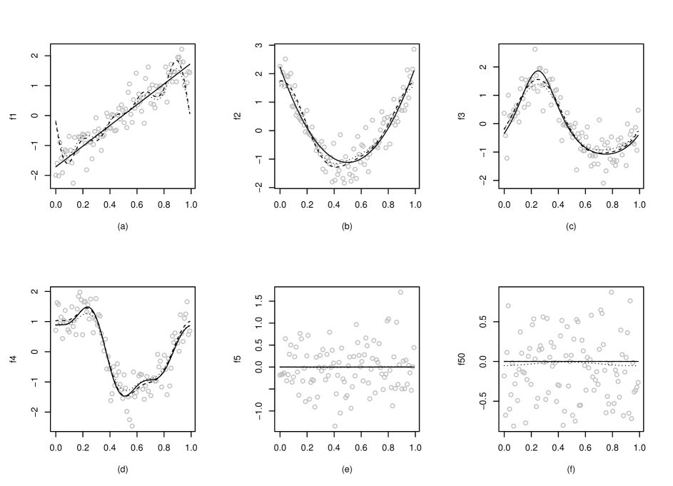
Figure 2: Examples of MAP (dashed lines) and SPAM (dotted lines) estimators for various $f_{j}$ (solid lines): $f_{1}$ (a), (b) $f_{2}$ (b), $f_{3}$ (c), $f_{4}$ (d) and two zero $f_{j}$ (e)-(f) ($SNR=5$).

The results in Table 1 show that MAP consistently outperforms SPAM (even with the oracle choices for $\lambda$) both globally and for each individual component $f_{j}$. For both methods the main contribution to the global AMSE came from estimating nonzero $f_{j}$. The MAP estimator almost perfectly identified the set of nonzero $f_{j}$ while the oracle choices for $\lambda$ in SPAM were quite small and, as a result, too many $\hat{f}_{j}$ were nonzero (see, e.g., Figure 2 (f)). In fact, it is a known common phenomenon for lasso-type estimators.

5 Concluding remarks

We considered sparse additive regression on a regular lattice, where the univariate components $f_{j}$ of the unknown response function $f$ belong to Sobolev balls. We established the minimax convergence rates of estimating $f$ and proposed an adaptive Fourier-based estimator which is rate-optimal over the entire range of Sobolev classes of different sparsity and smoothness. The resulting estimator was developed within Bayesian formalism but can also be viewed, in fact, as a penalized maximum likelihood estimator of the Fourier coefficients of $f$ with certain complexity penalties on the number of nonzero $f_{j}$ and on the numbers of nonzero entries of their Fourier coefficients $c_{j}$. It can be efficiently computed and the presented simulation study demonstrates its good performance.

The results of the paper can be extended to more general Besov classes of functions using the wavelet series expansions of $f_{j}$. The corresponding vectors of wavelet coefficients will lie then within weak $l_{p}$-balls (e.g., Johnstone, 2013, Section 9.7) and one can apply the results of Abramovich & Grinshtein (2013) for estimating a sparse group of sparse vectors from weak $l_{p}$-balls. The extension is quite straightforward though the details should be worked out. In particular, the resulting MAP estimator should mimic (hard) thresholding within each nonzero vector of wavelet coefficients instead of truncation as in the considered case of Fourier series (see Abramovich & Grinshtein, 2013).

Appendix

Throughout the proofs we use $C$ to denote a generic positive constant, not necessarily the same each time it is used, even within a single equation. Similarly, $C(\gamma)$ is a generic positive constant depending on $\gamma$.

Proof of Proposition 1

As we have mentioned before, the proposed sparse additive MAP estimator (12) can be equivalently viewed a penalized maximum likelihood estimator with complexity penalties (13) and (14). We can apply then the general results of Birge & Massart (2001) for complexity penalized estimators.

Rewrite first the model (8) in a different form. Set $\xi=\left(\xi_{-(n_{1}-1)/2,1},\ldots,\xi_{(n_{1}-1)/2,1},\ldots,\xi_{-(n_{d}-1)/2,d},\ldots,\xi_{(n_{d}-1)/2,d}\right)^{t}$ to be an amalgamated vector of length $N_{0}=\sum_{j=1}^{d}n_{j}$ of $d$ vectors $\xi_{1},\ldots,\xi_{d}$. Similarly, define $N_{0}$-dimensional amalgamated vectors $c=\left(c_{-(n_{1}-1)/2,1},\ldots,c_{(n_{1}-1)/2,1},\ldots,c_{-(n_{d}-1)/2,d},\ldots,c_{(n_{d}-1)/2,d}\right)^{t}$ and $z=\left(z_{-(n_{1}-1)/2,1},\ldots,z_{(n_{1}-1)/2,1},\ldots,z_{-(n_{d}-1)/2,d},\ldots,z_{(n_{d}-1)/2,d}\right)^{t}$. The original model (8) can be rewritten then as

$$\xi_{i}=c_{i}+\frac{\sigma^{2}}{N}z_{i},\quad i=1,\ldots,N_{0}$$ (22)

where $z_{i}$ are independent standard complex normal variates. Define an indicator vector $v$ by $v_{i}=\mathbb{\mathbb{I}}\left\{c_{i}\neq 0\right\}$, $i=1,\ldots,N_{0}$. Thus, in terms of model (22), $k_{j}=(1/2)\sum_{i=S_{j-1}+1}^{S_{j}}v_{i}$, where $S_{j}=\sum_{l=1}^{j-1}n_{l}$, and $d_{0}=\#\{j:k_{j}>0\}$. For a given $v$, let $D_{v}=2\sum_{j=1}^{d}k_{j}=\#\left\{i:\,v_{i}=1,\;i=1,\ldots,N_{0}\right\}$ be the overall number of nonzero entries of $c$, and define

$$L_{v}=\begin{cases}\frac{1}{D_{v}}\left\{\sum_{j=1}^{d}\log\left(\pi_{j}^{-1}\left(k_{j}\right)\right)+\log\left(\pi_{0}^{-1}\left(d_{0}\right)\binom{d}{d_{0}}\right)\right\}&\mbox{if}\>v\neq 0\\ \\ \log\pi_{0}^{-1}(0)&\mbox{if}\>v=0.\end{cases}$$ (23)

In the above notations the sparse additive MAP estimator $\hat{c}=\left(\hat{c}_{-(n_{1}-1)/2,1},\ldots,\hat{c}_{(n_{1}-1)/2,1},\ldots,\hat{c}_{-(n_{d}-1)/2,d},\ldots,\hat{c}_{(n_{d}-1)/2,d}\right)^{t}$ is the penalized maximum likelihood estimator of $c$ with the complexity penalty

$$Pen(v) = 2\frac{\sigma^{2}}{N}\left(1+\frac{1}{\gamma}\right)\left\{\sum_{j=1}^{d}\log\left(\pi_{j}^{-1}\left(k_{j}\right)\left(1+\gamma\right)^{k_{j}}\right)+\log\left(\pi_{0}^{-1}\left(d_{0}\right)\binom{d}{d_{0}}\right)\right\}$$ (24)

$$= 2\frac{\sigma^{2}}{N}\left(1+\frac{1}{\gamma}\right)D_{v}\left(L_{v}+\frac{1}{2}\log\left(1+\gamma\right)\right)$$

for $v\neq 0$, and $Pen(0)=2\frac{\sigma^{2}}{N}\left(1+\frac{1}{\gamma}\right)L_{0}$.

One can easily verify that

$$\sum_{v\neq 0}\exp\left\{-D_{v}L_{v}\right\}=\sum_{k=1}^{d}\pi_{0}(k)=1-\pi_{0}(0).$$

Furthermore, straightforward calculus similar to that in the proof of Theorem 1 of Abramovich et al. (2007) implies that under the conditions on the priors $\pi_{j}(\cdot)$ of Proposition 1, the complexity penalty $Pen(v)$ in (24) satisfies

$$Pen(v)\geq C(\gamma)\frac{\sigma^{2}}{N}D_{v}\left(1+\sqrt{2L_{v}}\right)^{2},\quad$$

for some $C(\gamma)>1$. One can then apply Theorem 2 of Birge & Massart (2001) to have

$$\sum_{j=1}^{d}E\left(\|\hat{c}_{j}-c_{j}\|_{2}^{2}\right) \leq c_{1}(\gamma)\min_{{\cal J}_{0}\subseteq\{1,\ldots,d\}}\left\{\sum_{j\in{\cal J}_{0}^{c}}\min_{1\leq k_{j}\leq(n_{j}-1)/2}\left(\sum_{k:|k|>k_{j}}|c_{kj}|^{2}+Pen_{j}\left(k_{j}\right)\right)\right.$$

$$\left.+\sum_{j\in{\cal J}_{0}}\sum_{|k|=1}^{(n_{j}-1)/2}|c_{kj}|^{2}+Pen_{0}\left(d_{0}\right)\right\}+c_{2}(\gamma)\frac{\sigma^{2}}{N}\left(1-\pi_{0}(0)\right).$$

Parseval’s equality $AMSE(\hat{f},f)=\sum_{j=1}^{d}E\left(\|\hat{c}_{j}-c_{j}\|_{n_{j}}^{2}\right)+\frac{\sigma^{2}}{N}$ completes the proof.

∎

Proof of Theorem 1

Let ${\cal J}_{0}^{c*}$ be the true (unknown) subset of nonzero $c_{j}$ and $d_{0}^{*}=|{\cal J}_{0}^{c*}|$. Consider separately two cases.

Case 1: $d_{0}^{*}\leq\lfloor d/e\rfloor$. Applying the general upper bound established in Proposition 1 for ${\cal J}_{0}={\cal J}_{0}^{*}$ yields

$$\begin{split}AMSE(\hat{f},f)&\leq C_{1}(\gamma)\left\{\sum_{j\in{\cal J}_{0}^{c*}}\min_{1\leq k_{j}\leq(n_{j}-1)/2}\left\{\sum_{|k|=k_{j}+1}^{(n_{j}-1)/2}|c_{kj}|^{2}+Pen_{j}(k_{j})\right\}+Pen_{0}(d_{0}^{*})\right\}\\ &+C_{2}(\gamma)\frac{\sigma_{2}}{N}\{1-\pi_{0}(0)\}.\end{split}$$ (25)

Choose the cut-points $k_{j}=\left\lfloor\frac{1}{2}\min(N^{\frac{1}{2s_{j}+1}},n_{j}-1)\right\rfloor$ for $j\in{\cal J}_{0}^{c*}$. If $k_{j}<(n_{j}-1)/2$, for $c_{j}\in\Theta_{n_{j}}(s_{j},R_{j})$ we have $\sum_{|k|=k_{j}+1}^{(n_{j}-1)/2}|c_{kj}|^{2}=O(k_{j}^{-2s_{j}})=O\left(N^{-\frac{2s_{j}}{2s_{j}+1}}\right)$, while for $k=(n_{j}-1)/2$, this term obviously disappears. Furthermore, under the conditions on the priors $\pi_{j}(\cdot)$, the corresponding penalties $Pen_{j}(\cdot)$ in (14) are of the AIC-type, where $Pen_{j}(k_{j})\sim 2C(\gamma)\frac{\sigma^{2}}{N}k_{j}=O\left(\min\left(N^{-\frac{2s_{j}}{2s_{j}+1}},\frac{n_{j}}{N}\right)\right)$. Hence, the first term $\sum_{j\in{\cal J}_{0}^{c*}}$ in the RHS of (25) is of the order $\sum_{j\in{\cal J}_{0}^{c*}}\min\left(N^{-\frac{2s_{j}}{2s_{j}+1}},\frac{n_{j}}{N}\right)$.

Finally, $\binom{d}{d^{*}_{0}}\leq\left(\frac{d}{d^{*}_{0}}\right)^{2d^{*}_{0}}$ for $d^{*}_{0}\leq\lfloor d/e\rfloor$ (see, e.g. Lemma A1 of Abramovich et al., 2010) and, therefore, the conditions on $\pi_{0}(\cdot)$ imply

$$Pen_{0}(d^{*}_{0})\leq C(\gamma)\frac{\sigma^{2}}{N}d_{0}^{*}\log(d/d_{0}^{*}).$$

Case 2: $\lfloor d/e\rfloor<d^{*}_{0}\leq d$. In this case we apply Proposition 1 for ${\cal J}_{0}=\emptyset$. Evidently, $|{\cal J}_{0}^{c}|=d$ and ${\cal J}_{0}^{c}={\cal J}_{0}^{*}\bigcup{\cal J}_{0}^{c*}$. Choose the cut-points $k_{j}=\left\lfloor\frac{1}{2}\min(N^{\frac{1}{2s_{j}+1}},n_{j}-1)\right\rfloor$ for $j\in{\cal J}_{0}^{c*}$ as before and $k_{j}=1$ for $j\in{\cal J}_{0}^{*}$. Then,

$$\begin{split}AMSE(\hat{f},f)&\leq C_{1}(\gamma)\left\{\sum_{j\in{\cal J}_{0}^{c*}}\left\{\sum_{|k|=k_{j}+1}^{(n_{j}-1)/2}|c_{kj}|^{2}+Pen_{j}(k_{j})\right\}+\sum_{j\in{\cal J}_{0}^{*}}Pen_{j}(1)+Pen_{0}(d)\right\}\\ &+C_{2}(\gamma)\frac{\sigma_{2}}{N}\{1-\pi_{0}(0)\}.\end{split}$$

We already showed that the first term $\sum_{j\in{\cal J}_{0}^{c*}}$ in the RHS of (Proof of Theorem 1) is $O\left(\sum_{j\in{\cal J}_{0}^{c*}}\min(N^{-\frac{2s_{j}}{2s_{j}+1}},\frac{n_{j}}{N}\right)$. The conditions of $\pi_{j}(1)$ and $\pi_{0}(d)$ imply that both $\sum_{j\in J_{0}^{*}}Pen_{j}(1)$ and $Pen_{0}(d)$ are $O(d/N)$, and, therefore, the first term in (Proof of Theorem 1) is dominating when $d^{*}_{0}\sim d$. ∎

Proof of Proposition 2

Consider the model (7) and the equivalent Gaussian sequence model (8) in the Fourier domain. Evidently, $\inf_{\tilde{f}_{j}}\sup_{f_{j}\in{\cal F}_{n_{j}}(s_{j},R_{j})}AMSE(\tilde{f}_{j},f_{j})=\inf_{\tilde{c}_{j}}\sup_{c_{j}\in\Theta_{n_{j}}(s_{j},R_{j})}E||\tilde{c}_{j}-c_{j}||^{2}_{n_{j}}$, where $\tilde{c}_{j}$ are discrete Fourier coefficients of $\tilde{f}_{j}$.

Most of the proof is a direct consequence of the standard techniques for establishing minimax lower bounds in the Gaussian sequence model over Sobolev ellipsoids (see, e.g. Tsybakov, 2009, Section 3.2) but unlike the standard setup, the variance in the considered model (8) depends on the sample size $N$ that may affect the minimax rates.

Consider the class of diagonal linear estimators $\tilde{c}_{j}(\lambda)$ of the form $\tilde{c}_{kj}=\lambda_{k}\xi_{kj},\;k=-(n-1)_{j}/2,\ldots,-1,1,\ldots,(n_{j}-1)/2$ and $\tilde{c}_{0j}=0$ (see Section 2.1). It is well known (see, e.g., Tsybakov, 2009, Section 3.2), that as $n_{j}$ tends to infinity, the minimax linear diagonal estimator is asymptotically minimax over all estimators of $f_{j}$:

$$\begin{split}\inf_{\tilde{c}_{j}}\sup_{c_{j}\in\Theta_{n_{j}}(s_{j},R_{j})}E||\tilde{c}_{j}-c_{j}||^{2}_{n_{j}}&\sim\inf_{\lambda}\sup_{c_{j}\in\Theta_{n_{j}}(s_{j},R_{j})}E||\tilde{c}_{j}(\lambda)-c_{j}||^{2}_{n_{j}}\\ &=\sup_{c_{j}\in\Theta_{n_{j}}(s_{j},R_{j})}\inf_{\lambda}E||\tilde{c}_{j}(\lambda)-c_{j}||^{2}_{n_{j}}.\end{split}$$

By standard calculus (see, e.g., Tsybakov, 2009, Section 3.2),

$$\inf_{\lambda}E||\tilde{c}_{j}(\lambda)-c_{j}||^{2}_{n_{j}}=\frac{\sigma^{2}}{N}\sum_{k=-(n_{j}-1)/2}^{(n_{j}-1)/2}\frac{|c_{kj}|^{2}}{|c_{kj}|^{2}+\frac{\sigma^{2}}{N}}$$ (26)

and the minimax linear estimator $\hat{c}_{j}^{L}$ is then of the form

$$\hat{c}^{L}_{kj}=(1-k^{s_{j}}\kappa_{j})_{+}\xi_{kj},$$

where $\kappa_{j}$ is the solution of the equation

$$\frac{\sigma^{2}}{N}\sum_{k=1}^{(n_{j}-1)/2}(2k)^{s_{j}}(1-(2k)^{s_{j}}\kappa_{j})_{+}=\kappa_{j}R_{j}^{2}.$$

Consider two cases:
a) $2s_{j}+1\geq\ln N/\ln n_{j}$. In this case we can follow Tsybakov (2009, Section 3.2) to get

$$\frac{\sigma^{2}}{N}\sum_{k=1}^{(n_{j}-1)/2}(2k)^{s_{j}}(1-(2k)^{s_{j}}\kappa_{j})_{+}=\frac{\sigma^{2}}{N}\sum_{k=1}^{k_{j}}(2k)^{s_{j}}(1-(2k)^{s_{j}}\kappa_{j}),$$ (27)

where $k_{j}=\lfloor\frac{1}{2}\kappa_{j}^{-1/s_{j}}\rfloor$, and neglecting the constants, $\kappa^{2}_{j}=N^{-\frac{2s_{j}}{2s_{j}+1}}$ and $E||\hat{c}_{j}^{L}-c_{j}||^{2}_{n_{j}}=O\left(N^{-\frac{2s_{j}}{2s_{j}+1}}\right)$.

The condition $2s_{j}+1\geq\ln N/\ln n_{j}$ is necessary to ensure that the resulting $k_{j}=\frac{1}{2}N^{\frac{1}{2s_{j}+1}}\leq(n_{j}-1)/2$ in (27).

b) $2s_{j}+1<\ln N/\ln n_{j}$. In this case one can easily see that

$$\frac{\sigma^{2}}{N}\sum_{k=1}^{(n_{j}-1)/2}(2k)^{s_{j}}(1-(2k)^{s_{j}}\kappa_{j})_{+}=\frac{\sigma^{2}}{N}\sum_{k=1}^{(n_{j}-1)/2}(2k)^{s_{j}}(1-(2k)^{s_{j}}\kappa_{j}),$$

$\kappa_{j}^{2}=\frac{n_{j}}{N}$ and $E||\hat{c}_{j}^{L}-c_{j}||^{2}_{n_{j}}=O\left(\frac{n_{j}}{N}\right)$.

∎

Proof of Theorem 2

No estimator $\tilde{f}$ of $f$ in (3) can obviously perform better than that of an oracle that knows the true subsets ${\cal J}_{0}$ and ${\cal J}_{0}^{c}$ of zero and nonzero components $f_{j}$ of $f$. In this ideal case, one would certainly set $\hat{f}_{j}=0$ for all $j\in{\cal J}_{0}$ with no error and, therefore, due to the additivity of the AMSE, Proposition 2 yields

$$\begin{split}\inf_{\tilde{f}}\sup_{f_{j}\in{\cal F}_{n_{j}}(s_{j},R_{j}),j\in{\cal J}_{0}^{c}}AMSE(\tilde{f},f)&=\sum_{j\in{\cal J}_{0}^{c}}\inf_{\tilde{f}_{j}}\sup_{f_{j}\in{\cal F}_{n_{j}}(s_{j},R_{j})}AMSE(\tilde{f}_{j},f_{j})\\ &\geq C_{2}\sum_{j\in{\cal J}_{0}^{c}}\min\left(N^{-\frac{2s_{j}}{2s_{j}+1}},\frac{n_{j}}{N}\right)\end{split}$$

(see Proposition 4.16 of Johnstone, 2013).

Furthermore, since $\min\left(N^{-\frac{2s_{j}}{2s_{j}+1}},\frac{n_{j}}{N}\right)>N^{-1},\;j\in{\cal J}_{0}^{c}$, for $d_{0}>d/2$ one has

$$\frac{d_{0}\ln(d/d_{0})}{N}\leq\ln 2~{}\frac{d_{0}}{N}\leq\ln 2\sum_{j\in{\cal J}_{0}^{c}}\min\left(N^{-\frac{2s_{j}}{2s_{j}+1}},\frac{n_{j}}{N}\right)$$

and the first term in the RHS of (16) is dominating. Thus, to complete the proof we need to show that for $d_{0}\leq d/2$,

$$\inf_{\tilde{f}}\sup_{f_{j}\in{\cal F}_{n_{j}}(s_{j},R_{j}),j\in{\cal J}_{0}^{c}}AMSE(\tilde{f},f)=\inf_{\tilde{c}}\sup_{c_{j}\in\Theta_{n_{j}}(s_{j},R_{j}),\;j\in{\cal J}_{0}^{c}}||\tilde{c}-c||^{2}_{N_{0}}\geq C_{2}\frac{d_{0}\ln(d/d_{0})}{N},$$ (28)

where $N_{0}=\sum_{j=1}^{d}n_{j}$ and $c$ is an $N_{0}$-dimensional amalgam of $d$ $n_{j}$-dimensional vectors of discrete Fourier coefficients $c_{j}$ of $f_{j}$.

The proof is based on finding a subset ${\cal C}_{d_{0}}$ of $N_{0}$-dimensional amalgamated vectors $c$ with $d_{0}$ nonzero components $c_{j}\in\Theta_{n_{j}}(s_{j},R_{j})$ such that for any pair $c^{1},c^{2}\in{\cal C}_{d_{0}}$ and some constant $C>0$, $||c^{1}-c^{2}||^{2}_{N_{0}}\geq C\frac{\sigma^{2}}{N}d_{0}\ln(d/d_{0})$ and the Kullback-Leibler divergence $K(\mathbb{P}_{c^{1}},\mathbb{P}_{c^{2}})=\frac{||c^{1}-c^{2}||^{2}_{N_{0}}}{2\sigma^{2}/N}\leq(1/16)\ln{\rm card}({\cal C}_{d_{0}})$. The required result in (28) then follows immediately from Lemma A.1 of Bunea et al. (2007).

Define the subset ${\cal\tilde{V}}_{d_{0}}$ of all $d$-dimensional indicator vectors with $d_{0}$ entries of ones: ${\cal\tilde{D}}_{d_{0}}=\{v:v\in\{0,1\}^{d},\;||v||_{0}=d_{0}\}$. Lemma A.3 of Rigollet & Tsybakov (2011) implies that for $d_{0}\leq d/2$, there exists a subset ${\cal V}_{d_{0}}\subset{\cal\tilde{V}}_{d_{0}}$ such that for some constant $C_{0}>0$, $\ln{\rm card}({\cal V}_{d_{0}})\geq C_{0}d_{0}\ln(d/d_{0})$, and for any pair $v_{1},v_{2}\in{\cal V}_{d_{0}}$, the Hamming distance $\rho(v_{1},v_{2})=\sum_{j=1}^{d}\mathbb{I}\{v_{1j}\neq v_{2j}\}\geq C_{0}d_{0}$.

To any indicator vector $v\in{\cal V}_{d_{0}}$ assign the corresponding vector $c\in{\cal C}_{d_{0}}$ as follows. Let $\tilde{C}^{2}=(1/16)C_{0}\frac{\sigma^{2}}{N}\ln(d/d_{0})$. Define $c_{j}$ to be a zero vector if $v_{j}=0$ and to have two nonzero entries $c_{-1j}=c_{1j}=\tilde{C}/\sqrt{2}$ otherwise. Evidently, $c_{j}\in{\cal F}(s_{j},\tilde{C})\subset{\cal F}_{n_{j}}(s_{j},R_{j})$ for $v_{j}=1$ and ${\rm card}({\cal C}_{d_{0}})={\rm card}({\cal V}_{d_{0}})$.

For any pair $c^{1},c^{2}\in{\cal C}_{d_{0}}$ and the corresponding $v_{1},v_{2}\in{\cal V}_{d_{0}}$, we then have

$$\begin{split}||c^{1}-c^{2}||^{2}_{N_{0}}&=\tilde{C}^{2}\sum_{j=1}^{d}\mathbb{I}\{v_{1j}\neq v_{2j}\}\geq\tilde{C}^{2}\;C_{0}\;d_{0}=\frac{1}{16}\frac{\sigma^{2}}{N}C_{0}^{2}d_{0}\ln(d/d_{0}),\\ K(\mathbb{P}_{c^{1}},\mathbb{P}_{c^{2}})&=\frac{\tilde{C}^{2}}{2\sigma^{2}/N}\sum_{j=1}^{d}\mathbb{I}\{v_{1j}\neq v_{2j}\}\leq\frac{\tilde{C}^{2}d_{0}}{\sigma^{2}/N}\leq\frac{1}{16}\ln{\rm card}({\cal C}_{d_{0}}),\end{split}$$

which completes the proof. ∎

References

• [1] Abramovich, F. & Grinshtein, V. (2010). MAP model selection in Gaussian regression. Electron. J. Stat. 4, 932–949.
• [2] Abramovich, F. & Grinshtein, V. (2013). Estimation of a sparse group of sparse vectors. Biometrika 100, 335–370.
• [3] Abramovich, F., Grinshtein, V. & Pensky, M. (2007). On optimality of Bayesian testimation in the normal means problem. Ann. Statist. 35, 2261–2286.
• [4] Abramovich, F., Grinshtein, V., Petsa, A. & Sapatinas, T. (2010). On Bayesian testimation and its application to wavelet thresholding. Biometrika 97, 181–198.
• [5] Birgé, L. & Massart, P. (2001). Gaussian model selection. J. Eur. Math. Soc. 3, 203–268.
• [6] Bunea, F., Tsybakov, A. & Wegkamp, M.H. (2007). Aggregation for Gaussian regression. Ann. Statist. 35, 1674–1697.
• [7] Donoho, D.L. & Johnstone, I.M. (1994). Ideal spatial adaptation by wavelet shrinkage. Biometrika 81, 425–455.
• [8] Friedman, J. & Stuetzle, W. (1981). Projection pursuit regression. J. Amer. Statist. Assoc. 76, 817–823.
• [9] Guedj, B. & Alquier, P. (2013). PAC-Bayesian estimation and prediction in sparse additive models. Electron. J. Stat. 7, 264–291.
• [10] Hastie, T. & Tibshirani, R. (1990). Generalized Additive Models. Chapman & Hall, London.
• [11] Johnstone, I. M. (2013). Gaussian Estimation: Sequence and Multiresolution Models. http://statweb.stanford.edu/ imj/GE06-11-13.pdf
• [12] Korostelev, A. & Korosteleva, O. (2011). Mathematical Statistics: Asymptotic Minimax Theory. American Mathematical Society, Providence.
• [13] Koltchinskii, V. & Yuan, M. (2010). Sparsity in multiple kernel learning. Ann. Statist. 38, 3660–3695.
• [14] Lin, Y. & Zhang, H.H. (2006). Component selection and smoothing in multivariate nonparametric regression. Ann. Statist. 34, 2272–2297.
• [15] Meier, L., van de Geer, S. & Buhlmann, P. (2009). High-dimensional additive modelling. Ann. Statist. 37, 3779–3821.
• [16] Raskutti, G., Wainwright, M.J. & Yu, B. (2011). Minimax rates of estimations for high-dimensional regression over $l_{q}$ balls. IEEE Trans. Inform. Theory 57, 6976–6994.
• [17] Raskutti, G., Wainwright, M.J. & Yu, B. (2012). Minimax-optimal rates for sparse additive models over kernel classes via convex programming. J. Mach. Learn. Research 13, 389–427.
• [18] Ravikumar, P., Lafferty, J., Liu, H. & Wasserman, L. (2009). Sparse additive models. J.R. Statist. Soc. B 71, 1009-1030.
• [19] Rigollet, P. & Tsybakov, A. (2011). Exponential screening and optimal rates of sparse estimation. Ann. Statist. 39, 731-771.
• [20] Suzuki, T. (2012). PAC-Bayesian bound for Gaussian process regression and multiple kernel additive model. JMLR: Workshop and Conference Proceedings 23, 8.1–8.20
• [21] Suzuki, T. & Sugiyama (2013). Fast learning rate of multiple kernel learning: trade-off between sparsity and smoothness. Ann. Statist. 41, 1381–1405.
• [22] Tsybakov, A. (2009). Introduction to Nonparametric Estimation. Springer, New York.
• [23] Wahba, G. (1990). Spline Models for Observational Data. SIAM, Philadelphia.
• [24] Yuan, M. & Lin, Y. (2006). Model selection and estimation in regression with grouped variables. J.R. Statist. Soc. B 68, 49–67.