Properties and numerical evaluation of the Rosenblatt distribution

Abstract

This paper studies various distributional properties of the Rosenblatt distribution. We begin by describing a technique for computing the cumulants. We then study the expansion of the Rosenblatt distribution in terms of shifted chi-squared distributions. We derive the coefficients of this expansion and use these to obtain the Lévy–Khintchine formula and derive asymptotic properties of the Lévy measure. This allows us to compute the cumulants, moments, coefficients in the chi-square expansion and the density and cumulative distribution functions of the Rosenblatt distribution with a high degree of precision. Tables are provided and software written to implement the methods described here is freely available by request from the authors.

and

1 Introduction

Typical limits of normalized of sums of long-range dependent stationary series are Brownian motion, fractional Brownian motion or the Rosenblatt process. Brownian motion and fractional Brownian motion are Gaussian and can thus be readily tabulated. This is not the case for the Rosenblatt distribution. The goal of this paper is to fill this gap. The tables can be used to compute asymptotic confidence intervals and to implement maximum likelihood methods.

The Rosenblatt distribution is the simplest non-Gaussian distribution which arises in a non-central limit theorem involving long-range dependent random variables [11, 29, 30]. For an overview, see [31]. It also appears in a statistical context as the asymptotic distribution of certain estimators (e.g., [32]).

We shall begin by motivating the Rosenblatt distribution using Rosenblatt’s famous counterexample found in [19]. Consider a stationary Gaussian sequence $X_{i}$, $i=1,2,\ldots$ which has a covariance structure of the form $\mathbb{E}X_{0}X_{k}\sim k^{-D}$ as $k\rightarrow\infty$ with $0<D<1/2$. Using the transformation

$$Y_{i}=X_{i}^{2}-1,$$ (1)

one can define a sequence of normalized sums

$$Z_{D}^{N}=\frac{\sigma(D)}{N^{1-D}}\sum_{i=1}^{N}Y_{i}.$$ (2)

Here, $\sigma(D)$ is a normalizing constant and is given by

$$\sigma(D)=\bigl{[}{\textstyle\frac{1}{2}}(1-2D)(1-D)\bigr{]}^{1/2}.$$ (3)

The sequence $Z_{D}^{N}$ tends to a non-Gaussian limit $Z_{D}$ as $N\rightarrow\infty$ with mean $0$ and variance $1$. This limiting distribution was named the Rosenblatt distribution in [29]. The characteristic function of $Z_{D}$ can be given as the following power series which is only convergent near the origin:

$$\phi(\theta)=\exp\Biggl{(}\frac{1}{2}\sum_{k=2}^{\infty}(2\mathrm{i}\theta\sigma(D))^{k}\frac{c_{k}}{k}\Biggr{)},$$ (4)

where

$$c_{k}=\int_{0}^{1}\mathrm{d}x_{1}\int_{0}^{1}\mathrm{d}x_{2}\cdots\int_{0}^{1}\mathrm{d}x_{k}|x_{1}-x_{2}|^{-D}|x_{2}-x_{3}|^{-D}\cdots|x_{k-1}-x_{k}|^{-D}|x_{k}-x_{1}|^{-D}.$$ (5)

By Cauchy–Schwarz,

$$c_{k}\leq\biggl{(}\int_{0}^{1}\int_{0}^{1}|x_{1}-x_{2}|^{-2D}\,\mathrm{d}x_{1}\,\mathrm{d}x_{2}\biggr{)}^{k/2}=\biggl{(}\frac{1}{(1-2D)(1-D)}\biggr{)}^{k/2}=\biggl{(}\frac{1}{2\sigma^{2}(D)}\biggr{)}^{k/2},$$ (6)

ensuring that the series (4) converges around the origin. [Since (6) is an equality when $k=2$, $Z_{D}$ has variance $1$ in view of (4) and (3).]

It is interesting to consider the extremes when $D\rightarrow 0^{+}$ and $D\rightarrow\frac{1}{2}^{-}$. When $D\rightarrow 0^{+}$, notice that $c_{k}\rightarrow 1$ for all $k$, $\sigma(D)\rightarrow\frac{1}{\sqrt{2}}$ and thus for $\theta$ small enough, the characteristic function approaches

$$\phi(\theta) = \exp\Biggl{(}\frac{1}{2}\sum_{k=2}^{\infty}\frac{(\sqrt{2}\mathrm{i}\theta)^{k}}{k}\Biggr{)}$$

$$= \exp\biggl{(}\frac{1}{2}\bigl{(}\log\bigl{(}1-\sqrt{2}\mathrm{i}\theta\bigr{)}-\sqrt{2}\mathrm{i}\theta\bigr{)}\biggr{)}$$

$$= \biggl{(}\frac{1}{1-\sqrt{2}\mathrm{i}\theta}\biggr{)}^{1/2}\mathrm{e}^{-\mathrm{i}\theta/\sqrt{2}},$$

which is the characteristic function of $\frac{1}{\sqrt{2}}(\varepsilon^{2}-1)$, where $\varepsilon$ is $N(0,1)$. Hence when $D=0$, the Rosenblatt distribution is simply a chi-squared distribution standardized to have mean 0 and variance 1.

As $D\rightarrow\frac{1}{2}^{-}$, the limit is $N(0,1)$. This is not surprising given that the scaling term in (2) approaches $\sqrt{N}$, hence you would assume the usual central limit theorem to hold and the limiting distribution to be Gaussian. This fact is not obvious however from the characteristic function (4). In Section 4 of this work, we derive an alternative form of the characteristic function from which this Gaussian limit is easier to see.

The distribution $Z_{D}$ can be given in terms of a weighted sum of chi-squared distributions,

$$Z_{D}=\sum_{i=1}^{\infty}\lambda_{n}(\varepsilon_{n}^{2}-1),\qquad\varepsilon_{n}\mbox{ i.i.d. }N(0,1),$$ (8)

where the weights $\{\lambda_{n}\}_{n=1}^{\infty}$ are such that

$$\sum_{n=1}^{\infty}\lambda_{n}^{k}=\sigma^{k}(D)c_{k},\qquad k=2,3,\ldots.$$ (9)

The series (8) converges a.s. and in $L^{2}$ because

$$\sum_{n=1}^{\infty}\operatorname{Var}[\lambda_{n}(\varepsilon_{n}^{2}-1)] = \mathbb{E}[(\varepsilon_{1}^{2}-1)^{2}]\sum_{n=1}^{\infty}\lambda_{n}^{2}=2\sum_{n=1}^{\infty}\lambda_{n}^{2}<\infty.$$

In fact, $\sum_{n=1}^{\infty}\lambda_{n}^{2}=1/2$ by (5) and (3). The weights $\{\lambda_{n}\}$ are given as the eigenvalues of an integral operator which we will discuss in more detail in Section 3. Various integral representations can be found in [32]. Our main focus in this work is on distributional properties of this distribution, namely, cumulants, moments and obtaining a numerical evaluation of the Rosenblatt distribution. A table for the cumulative distribution function (CDF) of the Rosenblatt distribution is useful for obtaining percentiles and confidence intervals.

This paper is organized as follows: In Section 2, we look at the moments and cumulants of the Rosenblatt distribution, as well as detailing a method for computing them. In Section 3, we show that the $\lambda_{n}$’s in the expansion (8) are given by the eigenvalues of an integral operator, and we give asymptotic formulas for this sequence. In Section 4, we state the characteristic function of the Rosenblatt distribution in Lévy–Khintchine form and use it to derive further properties of the Rosenblatt distribution. In Section 6, we compute the moments, cumulants and the $\lambda_{n}$’s and in Section 7, the quantiles of the Rosenblatt distribution are computed for various $D$ values. For more details and software, see the supplemental article [35].

2 Cumulants and moments of the Rosenblatt distribution

It follows from the expansion of the characteristic function (4) around $\theta=0$ that the cumulants $\kappa_{k}$ of the Rosenblatt distribution are given by $\kappa_{1}=0$ and

$$\kappa_{k}=2^{k-1}(k-1)!(\sigma(D))^{k}c_{k},$$ (10)

where the $c_{k}$ are given by the multiple integrals (5). Each moment $\mu_{n}$, $n\geq 1$ can then be expressed as a polynomial using the cumulants $\kappa_{k}$, $k=1,2,\ldots,n$. These are the complete Bell Polynomials

$$\mu_{n}=B_{n}(0,\kappa_{2},\ldots,\kappa_{n})$$ (11)

as noted, for example, in [17, 18]. They can also be computed recursively [24].

Thus, in order to compute any moment or cumulant, it is necessary to compute the multiple integrals $c_{k}$. The first two can be computed directly,

$$c_{2} = \int_{0}^{1}\int_{0}^{1}|x_{1}-x_{2}|^{-2D}\,\mathrm{d}x_{1}\,\mathrm{d}x_{2}=2\int_{0}^{1}\int_{0}^{x_{2}}(x_{1}-x_{2})^{-2D}\,\mathrm{d}x_{1}\,\mathrm{d}x_{2}=\frac{1}{(1-2D)(1-D)},$$

$$c_{3} = \int_{0}^{1}\int_{0}^{1}\int_{0}^{1}|x_{1}-x_{2}|^{-D}|x_{2}-x_{3}|^{-D}|x_{3}-x_{1}|^{-D}\,\mathrm{d}x_{1}\,\mathrm{d}x_{2}\,\mathrm{d}x_{3}$$

$$= 3\int_{0}^{1}x_{3}^{3D}\int_{0}^{x_{3}}\int_{0}^{x_{3}}\biggl{|}\frac{x_{1}}{x_{3}}-\frac{x_{2}}{x_{3}}\biggl{|}^{-D}\biggl{(}1-\frac{x_{2}}{x_{3}}\biggr{)}^{-D}\biggl{(}1-\frac{x_{1}}{x_{3}}\biggr{)}^{-D}\,\mathrm{d}x_{1}\,\mathrm{d}x_{2}\,\mathrm{d}x_{3}$$

$$= 3\biggl{(}\int_{0}^{1}x_{3}^{-3D+2}\,\mathrm{d}x_{3}\biggr{)}\biggl{(}\int_{0}^{1}\int_{0}^{1}|u_{1}-u_{2}|^{-D}(1-u_{2})^{-D}(1-u_{1})^{-D}\,\mathrm{d}u_{1}\,\mathrm{d}u_{2}\biggr{)}$$

$$= \frac{2}{1-D}\int_{0}^{1}w_{2}^{-D}\int_{0}^{w_{2}}(w_{2}-w_{1})^{-D}w_{1}^{-D}\,\mathrm{d}w_{1}\,\mathrm{d}w_{2}$$

$$= \frac{2}{1-D}\biggl{(}\int_{0}^{1}w_{2}^{-3D+1}\,\mathrm{d}w_{2}\biggr{)}\biggl{(}\int_{0}^{1}v^{-D}(1-v)^{-D}\,\mathrm{d}v\biggr{)}$$

$$= \frac{2}{(1-D)(2-3D)}\beta(1-D,1-D),$$

where $\beta(a,b)=\int_{0}^{1}v^{a-1}(1-v)^{b-1}\,\mathrm{d}v$ is the beta function and we made the following changes of variables above: $u_{1}=x_{1}/x_{3},u_{2}=x_{2}/x_{3}$, $w_{1}=1-u_{1},w_{2}=1-u_{2}$ and $v=w_{1}/w_{2}$.

For $k\geq 4$, a closed form expression for $c_{k}$ could not be found, which means they must be computed numerically. Computing the multiple integrals directly is intractable due to the increasing number of singularities in the integrand. It is for this reason that we now develop a more sophisticated method for computing $c_{k}$.

Let $L^{2}(0,1)$ denote the Hilbert space of all real-valued measurable functions $f(x),0<x<1$, such that $\|f\|_{2}\equiv(\int_{0}^{1}f(x)^{2}\,\mathrm{d}x)^{1/2}<\infty$, together with the usual inner product $(f,g)\equiv\int_{0}^{1}f(x)g(x)\,\mathrm{d}x$. For $0<D<1/2$, define the integral operator $\mathcal{K}_{D}\mathchoice{\nobreak\,\colon}{\nobreak\,\colon}{\nobreak\,\colon\;}{\nobreak\,\colon\;}L^{2}(0,1)\rightarrow L^{2}(0,1)$ as

$$(\mathcal{K}_{D}f)(x)=\int_{0}^{1}|x-u|^{-D}f(u)\,\mathrm{d}u.$$ (13)

Finally, define the sequence of functions $G_{k,D}\in L^{2}(0,1)$, $k\geq 1$, recursively as follows:

$$G_{1,D}(x)=\frac{(1-x)^{-D}}{\sqrt{1-D}};\qquad G_{k,D}(x)=(\mathcal{K}_{D}G_{k-1,D})(x),\qquad k\geq 2.$$ (14)

Then, we have the following alternative way to express $c_{k}$.

Proposition 2.0

Let $\mu$ and $\nu$ be any two positive integers such that $\mu+\nu=k$. Then

$$c_{k}=(G_{\mu,D},G_{\nu,D}).$$ (15)

Proof.

Let $\mu,\nu$ be as stated. Then, using the circular symmetry of the integrand in (5), if we take $x_{k}$ as the largest of the $x_{i}$, $i=1,2,\ldots$ , and then factor an $x_{k}$ out of all the terms, we can rewrite $c_{k}$ as

$$c_{k} = k\int_{0}^{1}x_{k}^{-kD}\int_{(0,x_{k})^{k-1}}\biggl{(}1-\frac{x_{1}}{x_{k}}\biggr{)}^{-D}\biggl{|}\frac{x_{1}}{x_{k}}-\frac{x_{2}}{x_{k}}\biggr{|}^{-D}\ldots$$

$$\hphantom{k\int_{0}^{1}x_{k}^{-kD}\int_{(0,x_{k})^{k-1}}}{}\times\biggl{|}\frac{x_{k-2}}{x_{k}}-\frac{x_{k-1}}{x_{k}}\biggr{|}^{-D}\biggl{(}1-\frac{x_{k-1}}{x_{k}}\biggr{)}^{-D}\,\mathrm{d}x_{1}\cdots\,\mathrm{d}x_{k}.$$

With the change of variables $u_{i}=x_{i}/x_{k}$, $i=1,2,\ldots,k-1$, one of the $k$ integrals can be separated out, and we obtain

$$c_{k} = k\biggl{(}\int_{0}^{1}x_{k}^{-kD+(k-1)}\,\mathrm{d}x_{k}\biggr{)}$$

$${}\times\biggl{(}\int_{(0,1)^{k-1}}(1-u_{1})^{-D}|u_{1}-u_{2}|^{-D}\cdots|u_{k-1}-u_{k-2}|^{-D}(1-u_{k-1})^{-D}\,\mathrm{d}u_{1}\cdots\,\mathrm{d}u_{k-1}\biggr{)}$$

$$= \frac{1}{1-D}\biggl{(}\int_{(0,1)^{k-1}}(1-u_{1})^{-D}|u_{1}-u_{2}|^{-D}\cdots$$

$$\hphantom{\frac{1}{1-D}\biggl{(}\int_{(0,1)^{k-1}}}{}\times|u_{k-1}-u_{k-2}|^{-D}(1-u_{k-1})^{-D}\,\mathrm{d}u_{1}\cdots\,\mathrm{d}u_{k-1}\biggr{)}$$

$$= \int_{(0,1)^{k-1}}G_{1,D}(u_{1})\underbrace{|u_{1}-u_{2}|^{-D}\cdots|u_{k-1}-u_{k-2}|^{-D}}_{k-2\ \mathrm{terms}}G_{1,D}(u_{k-1})\,\mathrm{d}u_{1}\cdots\,\mathrm{d}u_{k-1}$$

$$= \int_{(0,1)^{k-3}}\biggl{[}\int_{0}^{1}G_{1,D}(u_{1})|u_{1}-u_{2}|^{-D}\,\mathrm{d}u1\biggr{]}[|u_{3}-u_{2}|^{-D}\cdots|u_{k-2}-u_{k-3}|^{-D}]$$

$$\hphantom{\int_{(0,1)^{k-3}}}{}\times\biggl{[}\int_{0}^{1}G_{1,D}(u_{k-1})|u_{k-1}-u_{k-2}|^{-D}\,\mathrm{d}u_{k-1}\biggr{]}\,\mathrm{d}u_{3}\cdots\,\mathrm{d}u_{k-2}$$

$$= \int_{(0,1)^{k-3}}G_{2,D}(u_{2})\underbrace{|u_{2}-u_{3}|^{-D}\cdots|u_{k-2}-u_{k-3}|^{-D}}_{k-4\ \mathrm{terms}}G_{2,D}(u_{k-2})\,\mathrm{d}u_{2}\cdots\,\mathrm{d}u_{k-2}$$

$$\vdots$$

$$= \int_{0}^{1}G_{\mu,D}(u_{\mu})G_{\nu,D}(u_{k-\nu})\,\mathrm{d}u_{\mu}=(G_{\mu,D},G_{\nu,D}).$$

This finishes the proof. ∎

To minimize the number of integrals one needs to compute, it makes sense to choose $\mu=\nu=\frac{k}{2}$ if $k$ is even, and $\mu=\frac{k+1}{2}$ and $\nu=\frac{k-1}{2}$ if $k$ is odd. Proposition 1 thus reduces the problem of computing a $k$-dimensional integral into computing $\lceil\frac{k}{2}\rceil+1$ one-dimensional integrals.

$G_{2,D}$ can be given in terms of the beta function and the Gauss hypergeometric function ${}_{2}F_{1}(a,b;c;x)$, which has the following integral representation,

$${}_{2}F_{1}(a,b;c;x)=\frac{\Gamma(c)}{\Gamma(b)\Gamma(c-b)}\int_{0}^{1}v^{b-1}(1-v)^{c-b-1}(1-xv)^{-a}\,\mathrm{d}v,$$

(17)

$$\quad x<1,c>b>0.$$

Indeed,

$$G_{2,D}(x) = \frac{1}{\sqrt{1-D}}\int_{0}^{1}(1-u)^{-D}|x-u|^{-D}\,\mathrm{d}u$$

$$= \frac{1}{\sqrt{1-D}}\biggl{[}\int_{0}^{x}(1-u)^{-D}(x-u)^{-D}\,\mathrm{d}u+\int_{x}^{1}(1-u)^{-D}(u-x)^{-D}\,\mathrm{d}u\biggr{]}$$

$$= \frac{1}{\sqrt{1-D}}\biggl{[}x^{1-D}\int_{0}^{1}(1-xv)^{-D}(1-v)^{-D}\,\mathrm{d}v$$

$$\hphantom{\frac{1}{\sqrt{1-D}}\biggl{[}}{}+(1-x)^{1-2D}\int_{0}^{1}w^{-D}(1-w)^{-D}\,\mathrm{d}w\biggr{]}$$

$$= \frac{1}{\sqrt{1-D}}\biggl{[}\frac{x^{1-D}}{1-D}{}_{2}F_{1}(D,1,2-D,x)+(1-x)^{1-2D}\beta(1-D,1-D)\biggr{]}$$

$$= \frac{x^{1-D}}{(1-D)^{3/2}}{}_{2}F_{1}(D,1,2-D,x)+\frac{(1-x)^{1-2D}\beta(1-D,1-D)}{\sqrt{1-D}},$$

where, in the third equality we used the change of variables $v=u/x$ and $w=(1-u)/(1-x)$, and in the fourth, we used (2). The function ${}_{2}F_{1}(a,b;c;x)$ is bounded for $x\in(0,1)$ as long as $c>a+b$ ([16], Section 60:7), which is true in this case. This implies that unlike $G_{1,D}$, $G_{2,D}$ is a bounded function on $(0,1)$, since $0<D<\frac{1}{2}$.

In Section C of the supplemental article [35], we outline a technique for computing the $c_{k}$ numerically based on Proposition 1, and tabulate the first 8 cumulants and moments of the Rosenblatt distribution for various values of $D$.

3 Eigenvalue expansion of the Rosenblatt distribution

In this section, we focus on the expansion of the Rosenblatt distribution in terms of shifted chi-squared distributions (8). The sequence $\{\lambda_{i}\}_{i=1}^{\infty}$ can be thought of in two ways.

One way is to start with the integrals $\{c_{k},k\geq 2\}$ defined in (5) and to view $\{\lambda_{i}\}_{i=1}^{\infty}$ as a non-increasing sequence related to these $\{c_{k},k\geq 2\}$ through formula (9), see [29]. While easier to state, this perspective sheds little light on the $\lambda_{i}$’s since the $c_{k}$’s are so complicated.

The second way to characterize the sequence $\{\lambda_{i}\}_{i=1}^{\infty}$ is more useful in our case, and stems from Proposition 2 in [11]. To recall this proposition, let $X$ be defined through the Wiener–Itô integral

$$X=\int^{\prime\prime}_{\mathbb{R}^{2}}H(x,y)Z_{G}(\mathrm{d}x)Z_{G}(\mathrm{d}y),$$ (19)

where $Z_{G}$ is a complex-valued random measure with control measure $G$ such that for all Borel sets $A\in\mathbb{R}$, $Z_{G}(A)=Z_{G}(-A)$ and $G(A)=G(-A)$, and the kernel $H(x,y)$ is a complex-valued measurable function such that $H(x,y)=H(y,x)=\overline{H(-x,-y)}$ for all $x,y\in\mathbb{R}$, and $\int_{\mathbb{R}^{2}}|H(x,y)|^{2}G(\mathrm{d}x)G(\mathrm{d}y)<\infty$. The double prime in the integral means to exclude the diagonal $\{x=\pm y\}$. For background on such integrals, see [17] or [15].

Let $L_{G}^{2}(\mathbb{R})$ denote the space of complex valued functions $h(x)$, $x\in\mathbb{R}$ such that for all $x\in\mathbb{R}$, $h(x)=\overline{h(-x)}$ and $\int|h(x)|^{2}G(\mathrm{d}x)<\infty$. For random variables $X$ defined as in (19), Dobrushin and Major showed that $X$ has an expansion

$$X=\sum_{n=1}^{\infty}\eta_{n}(\varepsilon_{n}^{2}-1),$$

where the sequence $\eta_{n}$ corresponds to the eigenvalues of the integral operator $A\mathchoice{\nobreak\,\colon}{\nobreak\,\colon}{\nobreak\,\colon\;}{\nobreak\,\colon\;}L_{G}^{2}(\mathbb{R})\rightarrow L_{G}^{2}(\mathbb{R}^{2})$ defined as

$$(Ah)(x)=\int_{-\infty}^{\infty}H(x,-y)h(y)G(\mathrm{d}y).$$ (20)

In [30], it is shown that the Rosenblatt distribution has the following representation as a Wiener–Itô integral:

$$Z_{D}=a(D)\int_{\mathbb{R}^{2}}^{\prime\prime}\frac{\mathrm{e}^{\mathrm{i}(x+y)}-1}{\mathrm{i}(x+y)}Z_{G_{D}}(\mathrm{d}x)Z_{G_{D}}(\mathrm{d}y),$$ (21)

where the measure $G_{D}$ is absolutely continuous and is given by

$$G_{D}(\mathrm{d}x)=|x|^{D-1}\,\mathrm{d}x,\qquad x\in\mathbb{R}.$$ (22)

The constant

$$a(D)=\frac{\sigma(D)}{2\Gamma(D)\sin((1-D)\uppi/2)},$$ (23)

where $\sigma(D)$ is given in (3), ensures a variance of 1.

Thus, Dobrushin and Major’s result implies that the sequence $\lambda_{n}$ we seek in (8) is given as the eigenvalues of the operator $A_{D}\mathchoice{\nobreak\,\colon}{\nobreak\,\colon}{\nobreak\,\colon\;}{\nobreak\,\colon\;}L^{2}_{G_{D}}(\mathbb{R})\rightarrow L^{2}_{G_{D}}(\mathbb{R})$ defined as

$$(A_{D}h)(x)=a(D)\int_{-\infty}^{\infty}\frac{\mathrm{e}^{\mathrm{i}(x-y)}-1}{\mathrm{i}(x-y)}h(y)G_{D}(\mathrm{d}y).$$ (24)

We shall now reexpress the eigenvalue problem associated to (24) in a much simpler form so that we may both give analytical results about the $\lambda_{n}$’s and develop a method to compute them. This is done in the following proposition.

Proposition 3.0

The operators $A_{D}\mathchoice{\nobreak\,\colon}{\nobreak\,\colon}{\nobreak\,\colon\;}{\nobreak\,\colon\;}L^{2}_{G_{D}}(\mathbb{R})\rightarrow L^{2}_{G_{D}}(\mathbb{R})$ defined in (24) and $\sigma(D)\mathcal{K}_{D}\mathchoice{\nobreak\,\colon}{\nobreak\,\colon}{\nobreak\,\colon\;}{\nobreak\,\colon\;}\break L^{2}(0,1)\rightarrow L^{2}(0,1)$ defined in (13) have the same eigenvalues.

Proof.

Let $\widehat{g}(z)=(\mathcal{F}g)(z)=\int_{\mathbb{R}}g(y)\mathrm{e}^{\mathrm{i}yz}\,\mathrm{d}x$ and $\check{g}(z)=(\mathcal{F}^{-1}g)(z)=\frac{1}{2\uppi}\int_{\mathbb{R}}\mathrm{e}^{-\mathrm{i}xz}g(y)\,\mathrm{d}y$ denote the Fourier transform and inverse Fourier transfrom. Recall that $\mathcal{F}$ and $\mathcal{F}^{-1}$ are defined on $L^{1}(\mathbb{R})$ and $L^{2}(\mathbb{R})$ and can also be extended to generalized functions ([36], Chapter 7).

Let $(\lambda,h)$ be an eigenpair of the operator $A_{D}$. This implies that $h\in L_{G_{D}}^{2}(\mathbb{R})$ and thus $\int h(y)^{2}|y|^{D-1}\,\mathrm{d}y<\infty$ by (22). Taking inverse Fourier transforms of both sides in $\lambda h=A_{D}h$, we obtain

$$\lambda\check{h}=\mathcal{F}^{-1}(A_{D}h)=a(D)\mathcal{F}^{-1}(H_{1}*H_{2}),$$ (25)

where

$$H_{1}(y)=\bigl{(}\exp(\mathrm{i}y)-1\bigr{)}/(\mathrm{i}y)$$

and

$$H_{2}(y)=|y|^{D-1}h(y).$$

We want to apply the convolution theorem to compute the inverse Fourier transform in (25), however some care must be taken, because, while $H_{1}\in L^{1}(\mathbb{R})\cap L^{2}(\mathbb{R})$, $H_{2}$ is not necessarily in either $L^{1}(\mathbb{R})$ or $L^{2}(\mathbb{R})$. However, this difficulty can be avoided by writing $H_{2}$ as a sum:

$$H_{2}(y)=|y|^{D-1}h(y)\mathbf{1}_{[-1,1]}(y)+|y|^{D-1}h(y)\mathbf{1}_{(1,\infty)}(|y|):=H_{2}^{-}(y)+H_{2}^{+}(y).$$

Since $\int h(y)^{2}|y|^{D-1}\,\mathrm{d}y<\infty$, we have

$$H_{2}^{-}(y)=|y|^{D-1}h(y)\mathbf{1}_{[-1,1]}(y)\in L^{1}(\mathbb{R})$$

and

$$H_{2}^{+}(y)=|y|^{D-1}h(y)\mathbf{1}_{(1,\infty)}(|y|)\in L^{2}(\mathbb{R}).$$

By linearity of the convolution and Fourier transform, we can apply the convolution theorem for $L^{1}$ functions ([27], Proposition 6.2.1) and the convolution theorem for $L^{2}$ functions ([27], Proposition 6.5.3), we have

$$\lambda\check{h} = a(D)\mathcal{F}^{-1}(H_{1}*H_{2})=a(D)[\mathcal{F}^{-1}(H_{1}*H_{2}^{-})+\mathcal{F}^{-1}(H_{1}*H_{2}^{+})]$$

$$= 2\uppi a(D)\mathbf{1}_{(0,1)}(\check{H}_{2}^{-}+\check{H}_{2}^{+})=2\uppi a(D)\mathbf{1}_{(0,1)}\check{H}_{2},$$

where we have used the fact that $\check{H_{1}}=\mathbf{1}_{(0,1)}$ and we have picked up an extra factor of $2\uppi$ since we are applying the inverse Fourier transform $\mathcal{F}^{-1}$ to the convolution. This implies that for any eigenfunction $h$ of $A_{D}$, the support of $\check{h}$ is contained in $(0,1)$. Viewing $H_{2}$ as the product of $|y|^{D-1}$ and $h(y)$, we again apply the convolution theorem. Again, care must be taken as $|y|^{D-1}$ is not integrable or square integrable, but if we view $h$ and $|y|^{D-1}$ as generalized functions, the convolution theorem still applies since $\check{h}$ has compact support ([36], Theorem 7.9-1). Thus,

$$h(y)|y|^{D-1}=\mathcal{F}\bigl{(}\check{h}*\mathcal{F}^{-1}(|y|^{D-1})\bigr{)}.$$

Using this, we have

$$2\uppi a(D)\mathbf{1}_{(0,1)}\check{H}_{2} = 2\uppi a(D)\mathbf{1}_{(0,1)}\mathcal{F}^{-1}[h(y)|y|^{D-1}]$$

$$= 2\uppi a(D)\mathbf{1}_{(0,1)}\mathcal{F}^{-1}\bigl{[}\mathcal{F}\bigl{(}\check{h}*\mathcal{F}^{-1}(|y|^{D-1})\bigr{)}\bigr{]}$$

$$= 2\uppi a(D)\mathbf{1}_{(0,1)}\bigl{(}\check{h}*\mathcal{F}^{-1}(|y|^{D-1})\bigr{)}.$$

The inverse Fourier transform of $|y|^{D-1}$ is given by ([13], page 1119),

$$(\mathcal{F}^{-1}|y|^{D-1})(z)=\frac{1}{2\uppi}\biggl{[}2\Gamma(D)\sin\biggl{(}\frac{(1-D)\uppi}{2}\biggr{)}|z|^{-D}\biggr{]}=\frac{\sigma(D)}{2\uppi a(D)}|z|^{-D}$$ (26)

from (23). Thus, if $(h,\lambda)$ is an eigenpair for $A_{D}$, then

$$\lambda\check{h}(z) = (\mathcal{F}^{-1}A_{D}h)(z)$$

$$= \sigma(D){\bm{1}}_{[0,1]}(z)\int_{-\infty}^{\infty}|z-y|^{-D}\check{h}(y)\,\mathrm{d}y$$

$$= \sigma(D){\bm{1}}_{[0,1]}(z)\int_{0}^{1}|z-y|^{-D}\check{h}(y)\,\mathrm{d}y,$$

where we have again used the fact that $\check{h}$ is supported on $(0,1)$. Thus, if $(\lambda,h)$ is an eigenpair for $A_{D}$, then $(\lambda,\check{h}|_{(0,1)})$ is an eigenpair for $\sigma(D)\mathcal{K}_{D}$. Reversing this argument shows that there is a one-to-one correspondence between eigenpairs of $A_{D}$ and $\sigma_{D}\mathcal{K}$, which preserves the eigenvalues, hence these operators have the same eigenvalues. This completes the proof. ∎

The eigenvalues $\lambda_{n}$ of $\mathcal{K}_{D}$ are not known exactly, but their asymptotic behavior is well understood as $n\rightarrow\infty$, see for instance [12, 7, 14] or [20]. In particular, we have the following result regarding the asymptotic behavior of $\lambda_{n}$ in (8).

Theorem 3.1

Let $Z_{D}$ denote the Rosenblatt distribution given by

$$Z_{D}=\sum_{n=1}^{\infty}\lambda_{n}(D)(\varepsilon_{n}^{2}-1),\qquad\varepsilon_{n}\mbox{ i.i.d. }N(0,1),$$ (28)

where the non-increasing sequence $\{\lambda_{n}(D)\}$ is given by the eigenvalues of the integral operator $\sigma(D)\mathcal{K}_{D}\mathchoice{\nobreak\,\colon}{\nobreak\,\colon}{\nobreak\,\colon\;}{\nobreak\,\colon\;}L^{2}(0,1)\rightarrow L^{2}(0,1)$. The following asymptotic formula holds for any $0<r<1$:

$$\lambda_{n}(D)=C(D)n^{D-1}\biggl{(}1+\mathrm{o}\biggl{(}\frac{1}{n^{r}}\biggr{)}\biggr{)},$$ (29)

where,

$$C(D)=\frac{2}{\uppi^{1-D}}\sigma(D)\Gamma(1-D)\sin\biggl{(}\frac{\uppi D}{2}\biggr{)}.$$ (30)

Moreover, the series

$$\sum_{n=1}^{\infty}\bigl{(}\lambda_{n}(D)-C(D)n^{D-1}\bigr{)}$$

converges and equals

$$\sum_{n=1}^{\infty}\bigl{(}\lambda_{n}(D)-C(D)n^{D-1}\bigr{)}=-2^{1-D}\sigma(D)\zeta(D),$$ (31)

where $\zeta$ denotes the Riemann zeta function.

Proof.

Proposition 2 in [11] and Proposition 2 verify the first claim, namely that (28) holds and that the $\lambda_{n}$’s are the eigenvalues of $\sigma(D)\mathcal{K}_{D}$. Theorem 1 in [12] describes the eigenvalues of the operator $\int_{-1}^{1}|x-u|^{-D}f(u)\,\mathrm{d}y$. Thus, (29)–(31) follow immediately after noting that

$$\int_{-1}^{1}|z-u|^{-D}g(u)\,\mathrm{d}u=2^{1-D}\int_{0}^{1}|x-y|^{-D}f(y)\,\mathrm{d}y,$$

where $z=2x-1$, $u=2y-1$ and $g(u)=f(\frac{u+1}{2})$. ∎

Since Theorem 3.1 only gives the asymptotic behavior of the $\lambda_{n}$’s, we need to approximate those for which the asymptotic formula is not applicable. We present a method for approximating these eigenvalues in Section 6 (see also Section D of the supplemental article [35]).

4 Lévy–Khintchine representation of the Rosenblatt distribution

Recall that a distribution $X$ is infinitely divisible if for any integer $n\geq 1$, there exits $X_{i}^{(n)}$, $i=1,2,\ldots,n$, i.i.d. such that $X\stackrel{{\scriptstyle d}}{{=}}X_{1}^{(n)}+X_{2}^{(n)}+\cdots+X_{n}^{(n)}$. The characteristic function of an infinitely divisible distribution $X$ with $\mathbb{E}X^{2}<\infty$ can always be written in the following form:

$$\phi(\theta)=\mathbb{E}\mathrm{e}^{\mathrm{i}\theta X}=\exp\biggl{(}\mathrm{i}a\theta-\frac{1}{2}b^{2}\theta^{2}+\int_{-\infty}^{\infty}(\mathrm{e}^{\mathrm{i}\theta u}-1-\mathrm{i}u\theta)\nu(\mathrm{d}u)\biggr{)},$$

where $a\in\mathbb{R}$, $b>0$ and $\nu$ is a positive measure on $\mathbb{R}\setminus\{0\}$ with the property that $\int\min(u^{2},1)\*\nu(\mathrm{d}u)<\infty$. This is known as the Lévy Khintchine representation of $X$. Since the chi-square distribution is infinitely divisible, it is not surprising in light of (8) that the Rosenblatt distribution is also infinitely divisible. In this section, we will make this assertion rigorous, and give the Lévy Khintchine representation of the Rosenblatt distribution.

Before stating the result, we require first a lemma. Given any positive, increasing sequence $\mathbf{c}=\{c_{n}\}_{n=1}^{\infty}$ such that $\sum 1/c_{n}^{2}<\infty$, define the function $G_{\mathbf{c}}(x)$ for $0<x<1$ as

$$G_{\mathbf{c}}(x)=\sum_{n=1}^{\infty}x^{c_{n}}.$$ (32)

Since $\mathbf{c}^{-1}=\{c_{1}^{-1},c_{2}^{-1},\ldots\}\in\ell^{2}$, we have $c_{n}\rightarrow\infty$ and thus this series converges for all $x\in(0,1)$ since $\log x<0$ and hence for $n$ large enough, one has $x^{c_{n}}=\mathrm{e}^{c_{n}\log(x)}\leq c_{n}^{-2}.$ Notice that $G(0)=0$, $G_{\mathbf{c}}(x)\rightarrow\infty$ as $x\rightarrow 1$ and is a continuous function for all $x\in(0,1)$.

We now state a lemma regarding the asymptotic behavior of $G_{\mathbf{c}}$ as $x\rightarrow 0$ and $x\rightarrow 1$. In the following, we will say $a_{n}\sim b_{n}$ if $a_{n}/b_{n}\rightarrow 1$, and $a_{n}\lesssim b_{n}$ if $\limsup a_{n}/b_{n}\leq 1$.

Lemma 4.1

Suppose $\mathbf{c}$ is a positive strictly increasing sequence such that $c_{n}\sim\beta n^{\alpha}$ as $n\rightarrow\infty$ for some $1/2<\alpha<1$ and constant $\beta>0$. Then,

$$G_{\mathbf{c}}(x) \sim x^{c_{1}},\qquad\mbox{as }x\rightarrow 0,$$ (33)

$$G_{\mathbf{c}}(x) \sim \frac{1}{\alpha\beta^{1/\alpha}}\Gamma\biggl{(}\frac{1}{\alpha}\biggr{)}(1-x)^{-1/\alpha},\qquad\mbox{as }x\rightarrow 1.$$ (34)

Proof.

As $x\rightarrow 0$, we have

$$\frac{G_{\mathbf{c}}(x)}{x^{c_{1}}}=1+\sum_{n=2}^{\infty}x^{c_{n}-c_{1}}\rightarrow 1,$$ (35)

since $c_{n}>c_{1}$, so that the sum on the right hand side tends to 0. This confirms (33).

For the second assertion, let $0<\varepsilon<1$ and let $\beta^{\prime}=(1-\varepsilon)\beta$ and $\beta^{\prime\prime}=(1+\varepsilon)\beta$. By assumption, there exists $M$ large enough such that for $n\geq M$,

$$\beta^{\prime}n^{\alpha}<c_{n}<\beta^{\prime\prime}n^{\alpha}.$$ (36)

Let $G_{\mathbf{c}}^{(M)}(x)$ be the tail of the series $G_{\mathbf{c}}$:

$$G_{\mathbf{c}}^{(M)}(x)=\sum_{n=M}^{\infty}x^{c_{n}}.$$

Now, observe,

$$\int_{M}^{\infty}x^{(1+\varepsilon)\beta(y+1)^{\alpha}}\,\mathrm{d}y\leq\sum_{n=M}^{\infty}x^{\beta^{\prime\prime}n^{\alpha}}\leq G_{\mathbf{c}}^{(M)}(x)\leq\sum_{n=M}^{\infty}x^{\beta^{\prime}n^{\alpha}}\leq\int_{M}^{\infty}x^{(1-\varepsilon)\beta y^{\alpha}}\,\mathrm{d}y.$$ (37)

The integrals on the far ends of this inequality can be computed in terms of the upper incomplete gamma function $\Gamma(a,b)=\int_{b}^{\infty}z^{a-1}\mathrm{e}^{-z}\,\mathrm{d}z$, since for the right most integral,

$$\int_{M}^{\infty}x^{\beta^{\prime}y^{\alpha}}\,\mathrm{d}y = \int_{M}^{\infty}\mathrm{e}^{\beta^{\prime}y^{\alpha}\log(x)}\,\mathrm{d}y$$ (38)

$$= \frac{1}{\alpha}\frac{1}{(-\beta^{\prime}\log(x))^{1/\alpha}}\int_{-\beta^{\prime}\log(x)M^{\alpha}}^{\infty}u^{1/\alpha-1}\mathrm{e}^{-u}\,\mathrm{d}u$$ (39)

$$= \frac{(-\log(x))^{-1/\alpha}}{\alpha\beta^{\prime 1/\alpha}}\Gamma\biggl{(}\frac{1}{\alpha},-\beta^{\prime}\log(x)M^{\alpha}\biggr{)}.$$ (40)

And similarly, for the left most side of (37),

$$\int_{M}^{\infty}x^{\beta^{\prime\prime}(y+1)^{\alpha}}\,\mathrm{d}y=\int_{M-1}^{\infty}x^{\beta^{\prime\prime}y^{\alpha}}\,\mathrm{d}y=\frac{(-\log(x))^{-1/\alpha}}{\alpha\beta^{\prime\prime 1/\alpha}}\Gamma\biggl{(}\frac{1}{\alpha},-\beta^{\prime\prime}\log(x)(M-1)^{\alpha}\biggr{)}.$$ (41)

Using the following asymptotic expansion of $\Gamma(a,b)$ as $b\rightarrow 0$,

$$\Gamma(a,b)\sim\Gamma(a)-\frac{b^{a}}{a},\qquad a>0,\mbox{ as }b\rightarrow 0$$ (42)

(see [16], formula 45:9:7), and $\log(x)\sim x-1$ as $x\rightarrow 1$, (40) and (41) are asymptotic to

$$\frac{(1-x)^{-1/\alpha}}{\alpha\beta^{\prime 1/\alpha}}\Gamma\biggl{(}\frac{1}{\alpha}\biggr{)}\quad\mbox{and}\quad\frac{(1-x)^{-1/\alpha}}{\alpha\beta^{\prime\prime 1/\alpha}}\Gamma\biggl{(}\frac{1}{\alpha}\biggr{)},$$ (43)

respectively. Thus, (37) implies

$$\frac{1}{\alpha\beta^{\prime\prime 1/\alpha}}\Gamma\biggl{(}\frac{1}{\alpha}\biggr{)}(1-x)^{-1/\alpha}\lesssim G_{\mathbf{c}}^{(M)}(x)\lesssim\frac{1}{\alpha\beta^{\prime 1/\alpha}}\Gamma\biggl{(}\frac{1}{\alpha}\biggr{)}(1-x)^{-1/\alpha}$$ (44)

as $x\rightarrow 1$. Since everything is tending to $\infty$, (44) also holds with $G_{\mathbf{c}}^{(M)}(x)$ replaced with $G_{\mathbf{c}}(x)$. And finally, since $\varepsilon>0$ was arbitrary, we can let $\varepsilon\rightarrow 0$, making $\beta^{\prime},\beta^{\prime\prime}\rightarrow\beta$, which implies (34). ∎

We are now ready to give the Lévy Khintchine representation of the Rosenblatt distribution.

Theorem 4.2

Let $Z_{D}$ have a Rosenblatt distribution with $0<D<1/2$ and let

$$\mathbf{\lambda}(D)^{-1}=(\lambda_{1}(D)^{-1},\lambda_{2}(D)^{-1},\ldots)$$

be the sequence of the inverses of the eigenvalues associated to the integral operator $\sigma(D)\mathcal{K}_{D}$ defined in (13). Then the characteristic function of $Z_{D}$ can be written as

$$\phi(\theta)=\mathbb{E}\mathrm{e}^{\mathrm{i}\theta Z_{D}}=\exp\biggl{(}\int_{0}^{\infty}(\mathrm{e}^{\mathrm{i}\theta u}-1-\mathrm{i}\theta u)\nu_{D}(u)\,\mathrm{d}u\biggr{)},$$ (45)

where $\nu_{D}$ is supported on $(0,\infty)$ and is given by

$$\nu_{D}(u)=\frac{1}{2u}G_{\mathbf{\lambda}(D)^{-1}}(\mathrm{e}^{-u/2})=\frac{1}{2u}\sum_{n=1}^{\infty}\exp\biggl{(}-\frac{u}{2\lambda_{n}}\biggr{)},\qquad u>0.$$ (46)

Moreover, $\nu_{D}$ has the following asymptotic forms as $u\rightarrow 0^{+}$ and $u\rightarrow\infty$,

$$\nu_{D}(u) \sim \frac{2^{D/(1-D)}C(D)^{1/(1-D)}}{(1-D)}\Gamma\biggl{(}\frac{1}{1-D}\biggr{)}u^{(D-2)/(1-D)},\qquad u\rightarrow 0,$$ (47)

$$\nu_{D}(u) \sim \frac{\mathrm{e}^{-u/(2\lambda_{1})}}{2u},\qquad u\rightarrow\infty,$$ (48)

where $C(D)$ is defined in (30).

Proof.

Let

$$Z_{D}^{(M)}=\sum_{n=1}^{M}\lambda_{n}(\varepsilon_{i}^{2}-1).$$

We have $Z_{D}^{(M)}\stackrel{{\scriptstyle d}}{{\rightarrow}}Z_{D}$, and since $Z_{D}^{(M)}$ is a sum of shifted i.i.d. chi-squared distributions, we can use the Lévy Khintchine representation of a chi-square ([4], Example 1.3.22), which is a gamma distribution with shape parameter 1$/$2 and scale parameter 2:

$$\mathbb{E}\mathrm{e}^{\mathrm{i}\theta Z_{D}^{(M)}}=\prod_{n=1}^{M}\mathrm{e}^{\mathrm{i}\theta\lambda_{i}(\varepsilon_{i}^{2}-1)}=\prod_{n=1}^{M}\exp\biggl{(}-\mathrm{i}\theta\lambda_{i}+\int_{0}^{\infty}(\mathrm{e}^{\mathrm{i}\theta u}-1)\biggl{[}\frac{\mathrm{e}^{-u/(2\lambda_{i})}}{2u}\biggr{]}\,\mathrm{d}u\biggr{)}.$$ (49)

Using $(1/2)\int_{0}^{\infty}\mathrm{e}^{-u/(2\lambda)}\,\mathrm{d}u=\lambda,$ (49) can be rewritten as

$$\prod_{n=1}^{M}\exp\biggl{(}\int_{0}^{\infty}(\mathrm{e}^{\mathrm{i}\theta u}-1-\mathrm{i}\theta u)\biggl{[}\frac{\mathrm{e}^{-u/(2\lambda_{i})}}{2u}\biggr{]}\,\mathrm{d}u\biggr{)}$$

$$\quad=\exp\biggl{(}\int_{0}^{\infty}(\mathrm{e}^{\mathrm{i}\theta u}-1-\mathrm{i}\theta u)\biggl{[}\frac{1}{2u}G_{\lambda(D)^{-1}}^{(M)}(\mathrm{e}^{-u/2})\biggr{]}\,\mathrm{d}u\biggr{)},$$

where

$$G_{{\lambda(D)^{-1}}}^{(M)}(x)=\sum_{n=1}^{M}x^{\lambda_{i}^{-1}}.$$

Now, we let $M\rightarrow\infty$. In order to justify passing the limit though the integral, notice that

$$\biggl{|}(\mathrm{e}^{\mathrm{i}\theta u}-1-\mathrm{i}\theta u)\biggl{[}\frac{1}{2u}G_{\lambda(D)^{-1}}^{(M)}(\mathrm{e}^{-u/2})\biggr{]}\biggr{|}\leq\frac{\theta^{2}}{4}uG_{\lambda(D)^{-1}}^{(M)}(\mathrm{e}^{-u/2})\leq\frac{\theta^{2}}{4}uG_{\lambda(D)^{-1}}(\mathrm{e}^{-u/2}),$$ (50)

where we have used the identity $|\mathrm{e}^{\mathrm{i}z}-1-z|\leq\frac{z^{2}}{2}$ for $z\in\mathbb{R}$. Notice that (50) is continuous for $0<u<\infty$, and by (29) together with Lemma 4.1 using $\alpha=1-D$ and $\beta=C(D)^{-1}$, we have

$$uG_{\lambda(D)^{-1}}(\mathrm{e}^{-u/2})\sim u\mathrm{e}^{-u/(2\lambda_{1})}\qquad\mbox{as }u\rightarrow\infty$$ (51)

and,

$$uG_{\lambda(D)^{-1}}(\mathrm{e}^{-u/2})\sim C^{\prime}u(1-\mathrm{e}^{-u/2})^{-1/(1-D)}\sim C^{\prime\prime}u^{D/(1-D)}\qquad\mbox{as }u\rightarrow 0$$ (52)

for some constants $C^{\prime}$ and $C^{\prime\prime}$. Since $0<\frac{D}{1-D}<1$, (51) and (52) imply that (50) is integrable on $(0,\infty)$, and hence the dominated convergence theorem applies and

$$\mathbb{E}\mathrm{e}^{\mathrm{i}\theta Z_{D}^{(M)}}\rightarrow\mathbb{E}\mathrm{e}^{\mathrm{i}\theta Z_{D}}=\exp\biggl{(}\int_{0}^{\infty}(\mathrm{e}^{\mathrm{i}\theta u}-1-\mathrm{i}\theta u)\biggl{[}\frac{1}{2u}G_{\lambda(D)^{-1}}(\mathrm{e}^{-u/2})\biggr{]}\,\mathrm{d}u\biggr{)}$$

which verifies (45).

The final assertions (47) and (48) also follow from (29) and Lemma 4.1 with $\alpha=1-D$ and $\beta=C(D)^{-1}$, since these imply

$$\frac{1}{2u}G_{\lambda(D)^{-1}}(\mathrm{e}^{-u/2}) \sim \frac{1}{2u}\frac{C(D)^{-1/(1-D)}}{(1-D)}\Gamma\biggl{(}\frac{1}{1-D}\biggr{)}\biggl{(}\frac{u}{2}\biggr{)}^{-1/(1-D)}$$

$$= \frac{2^{D/(1-D)}C(D)^{1/(1-D)}}{(1-D)}\Gamma\biggl{(}\frac{1}{1-D}\biggr{)}u^{(D-2)/(1-D)},\qquad u\rightarrow 0$$

and

$$\frac{1}{2u}G_{\lambda(D)^{-1}}(\mathrm{e}^{-u/2})\sim\frac{1}{2u}\mathrm{e}^{-u/(2\lambda_{1})},\qquad u\rightarrow\infty.$$ (54)

This concludes the proof. ∎

Notice that for any $0<D<1/2$, the Lévy measure is normalized in the sense that

$$\int_{0}^{\infty}u^{2}\nu_{D}(u)\,\mathrm{d}u=\mathbb{E}Z_{D}^{2}=1.$$ (55)

As $D\rightarrow 1/2$, $\sigma(D)\rightarrow 0$ by (3) $\Rightarrow C(D)\rightarrow 0$ by (30) $\Rightarrow\lambda_{n}(D)\rightarrow 0$ by (29) $\Rightarrow\nu_{D}(u)\rightarrow 0$ by (46) and hence $u^{2}\nu_{D}(u)\rightarrow 0$ for all $u$ positive, but in light of (55), the function $u^{2}\nu_{D}(u)$ approaches a dirac mass at $u=0$. Thus, as $D\rightarrow 1/2$, since $(\mathrm{e}^{\mathrm{i}u\theta}-1-\mathrm{i}u\theta)\rightarrow-1/2\theta^{2}$, one gets

$$\phi(\theta)=\exp\biggl{(}\int_{0}^{\infty}\biggl{(}\frac{\mathrm{e}^{\mathrm{i}u\theta}-1-\mathrm{i}\theta u}{u^{2}}\biggr{)}u^{2}\nu_{D}(u)\,\mathrm{d}u\biggr{)}\rightarrow\exp\biggl{(}-\frac{1}{2}\theta^{2}\biggr{)},$$

which verifies that $Z_{D}\stackrel{{\scriptstyle d}}{{\rightarrow}}N(0,1)$.

Understanding the Lévy measure of a distribution has some immediate implications pertaining to its probability density function and distribution function. We will state three such results as corollaries. The first is not surprising given that $Z_{D}$ is an infinite sum of chi-squared distributions, however it is now easy to prove given what we know about the Lévy measure:

Corollary 4.3

For $0<D<1/2$, the probability density function of $Z_{D}$ is infinitely differentiable with all derivatives tending to $0$ as $|x|\rightarrow\infty$.

Proof.

Using Proposition 23.8 in [21], this follows as long as there exists an $\alpha\in(0,2)$ such that

$$\liminf_{r\rightarrow 0}\frac{\int_{[-r,r]}u^{2}\nu_{D}(u)\,\mathrm{d}u}{r^{2-\alpha}}>0.$$ (56)

And indeed, (47) implies that for some constant $\tilde{C}(D)$,

$$\int_{[-r,r]}u^{2}\nu_{D}(u)\,\mathrm{d}u\sim\tilde{C}(D)\int_{0}^{r}u^{-D/(1-D)}\,\mathrm{d}u=\tilde{C}(D)\biggl{(}\frac{1-D}{1-2D}\biggr{)}r^{2-1/(1-D)}.$$ (57)

Thus, choosing $\alpha=1/(1-D)$ verifies the result. ∎

The second corollary gives a simple bound on the left-hand tail of the CDF of $Z_{D}$. The proof is similar to Proposition 9.5(ii) in [28].

Corollary 4.4 ((Left tail))

Let $Z_{D}$ denote the Rosenblatt distribution. Then,

$$\mathrm{P}[Z_{D}<-x]\leq\exp\bigl{(}-{\textstyle\frac{1}{2}}x^{2}\bigr{)},\qquad x>0.$$ (58)

Proof.

For any $M\geq 1$, recall the random variable $Z^{(M)}_{D}$ defined in the proof of Theorem 4.2. Applying Markov’s inequality we see for any $x>0$ and $s>0$,

$$\mathrm{P}\bigl{(}Z^{(M)}_{D}\leq-x\bigr{)} \leq \mathrm{e}^{-sx}\mathbb{E}\mathrm{e}^{-sZ^{(M)}_{D}}$$

$$= \mathrm{e}^{-sx}\exp\biggl{(}\int_{0}^{\infty}(\mathrm{e}^{-su}-1+su)\,\mathrm{d}\nu^{(M)}(u)\,\mathrm{d}u\biggr{)},$$

where the last equality follows since $Z^{(M)}_{D}$ is a finite sum of weighted chi-square distributions, and hence has a moment generating function defined for $s<s_{0}$ for some $s_{0}>0$. Using the inequality $\mathrm{e}^{-su}-1+su\leq\frac{1}{2}s^{2}u^{2}$, and since $\nu^{(M)}(u)$ increases in $M$, (4) becomes

$$\mathrm{e}^{-sx}\exp\biggl{(}\int_{0}^{\infty}(\mathrm{e}^{-su}-1+su)\,\mathrm{d}\nu^{(M)}(u)\,\mathrm{d}u\biggr{)} \leq \mathrm{e}^{-sx}\exp\biggl{(}\frac{s^{2}}{2}\int_{0}^{\infty}u^{2}\nu^{(M)}(u)\,\mathrm{d}u\biggr{)}$$

$$\leq \mathrm{e}^{-sx}\exp\biggl{(}\frac{s^{2}}{2}\int_{0}^{\infty}u^{2}\nu(u)\,\mathrm{d}u\biggr{)}$$

$$\leq \exp\biggl{(}-sx+\frac{1}{2}s^{2}\biggr{)}$$

since $\operatorname{Var}Z_{D}=\int_{0}^{\infty}u^{2}\nu(u)\,\mathrm{d}u=1$. The minimum of (4) over $s$ is attained at $s=x$. Thus,

$$\mathrm{P}\bigl{(}Z^{(M)}_{D}\leq-x\bigr{)}\leq\exp\bigl{(}-{\textstyle\frac{1}{2}}x^{2}\bigr{)}$$ (61)

which finishes the proof. ∎

We obtain a result similar to Theorem 2 in [3] involving the rate of decay of the distribution function.

Corollary 4.5 ((Right tail))

Let $Z_{D}$ denote the Rosenblatt distribution. Then for $\alpha>0$,

$$\lim_{u\rightarrow\infty}\frac{\mathrm{P}[Z_{D}>u+\alpha]}{\mathrm{P}[Z_{D}>u]}=\mathrm{e}^{-\alpha/(2\lambda_{1})},$$

where $\lambda_{1}$ is the largest eigenvalue of $\sigma(D)\mathcal{K}_{D}$ defined in (13).

Proof.

For $u\geq 1$, define $\bar{A}_{\nu_{D}}$ as

$$\bar{A}_{\nu_{D}}(u)=\frac{\int_{u}^{\infty}\nu_{D}(v)\,\mathrm{d}v}{\int_{1}^{\infty}\nu_{D}(v)\,\mathrm{d}v}.$$

By Theorem 1 in [8], it suffices to show

$$\lim_{u\rightarrow\infty}\frac{\bar{A}_{\nu_{D}}(u+\alpha)}{\bar{A}_{\nu_{D}}(u)}=\mathrm{e}^{-\alpha/(2\lambda_{1})},$$ (62)

and

$$\int_{0}^{\infty}\mathrm{e}^{u/(2\lambda_{1})}\bar{A}_{\nu_{D}}(\mathrm{d}u)=\infty.$$ (63)

Both follow from (48) in Theorem 4.2. Indeed, as $u\rightarrow\infty$,

$$\int_{u}^{\infty}\nu_{D}(v)\,\mathrm{d}v\sim\int_{u}^{\infty}\frac{1}{2v}\mathrm{e}^{-v/(2\lambda_{1})}\,\mathrm{d}v\sim\frac{\lambda_{1}}{u}\mathrm{e}^{-u/(2\lambda_{1})}$$ (64)

which follows because

$$-\frac{\mathrm{d}}{\mathrm{d}x}\frac{\lambda_{1}}{u}\mathrm{e}^{-u/(2\lambda_{1})}=\frac{1}{2u}\mathrm{e}^{-u/(2\lambda_{1})}+\frac{\lambda_{1}}{u^{2}}\mathrm{e}^{-u/(2\lambda_{1})}\sim\frac{1}{2u}\mathrm{e}^{-u/(2\lambda_{1})},$$

and thus integrating both sides implies (64). From this, (62) follows. Also,

$$\int_{0}^{\infty}\mathrm{e}^{u/(2\lambda_{1})}\bar{A}_{\nu_{D}}(\mathrm{d}u) = \frac{1}{\int_{1}^{\infty}\nu_{D}(v)\,\mathrm{d}v}\int_{0}^{\infty}\mathrm{e}^{u/(2\lambda_{1})}\Biggl{(}\frac{1}{2u}\sum_{n=1}^{\infty}\mathrm{e}^{-u/(2\lambda_{n})}\Biggr{)}\,\mathrm{d}u$$

$$= \frac{1}{\int_{1}^{\infty}\nu_{D}(v)\,\mathrm{d}v}\int_{0}^{\infty}\frac{1}{2u}\Biggl{(}1+\sum_{n=1}^{\infty}\mathrm{e}^{-u/(2\lambda_{n})+u/(2\lambda_{1})}\Biggr{)}\,\mathrm{d}u=\infty,$$

since the integrand on the right is asymptotic to $1/(2u)$. This verifies (63). ∎

5 Approximating the distribution of the tail of the series

The representation of the Rosenblatt distribution $Z_{D}$ as an infinite sum of shifted chi-squared distributions (8) has proven to be quite useful for obtaining theoretical results about the distribution. In this section, we aim to take advantage of this representation to compute the CDF and PDF of the Rosenblatt distribution.

For $M\geq 1$, define $X_{M}$ and $Y_{M}$ as

$$Z_{D}=\sum_{n=1}^{M-1}\lambda_{n}(\varepsilon_{n}^{2}-1)+\sum_{n=M}^{\infty}\lambda_{n}(\varepsilon_{n}^{2}-1):=X_{M}+Y_{M}.$$ (65)

Notice that $Y_{M}$ has mean $0$ and variance

$$\sigma_{M}^{2}:=\mathbb{E}Y_{M}^{2}=2\sum_{n=M}^{\infty}\lambda_{n}^{2}.$$ (66)

Notice that from Theorem 3.1, as $M\rightarrow\infty$,

$$\sigma_{M}^{2}\sim 2C(D)^{2}\sum_{n=M}^{\infty}n^{2D-2}\sim 2C(D)^{2}(1-2D)^{-1}M^{2D-1},$$ (67)

where we approximated the sum $\sum_{n=M}^{\infty}\lambda_{n}^{2}$ with an integral. This suggests that $X_{M}$ alone is not a very good approximation of $Z_{D}$ since this variance tends to $0$ slowly with $M$, especially when $D$ is close to $1/2$. As an alternative, we will see below that $Y_{M}$ is approximated by a normal distribution as $M\rightarrow\infty$. By taking advantage of this property, we can obtain accurate approximations of the distribution of $Z_{D}$.

In [33], random variables expressed as infinite sums of gamma and hence chi-squared distributions were studied. It was shown in particular that the asymptotic form of the $\lambda_{n}$’s in the expansion implies that the distribution of the tail $Y_{M}$ is approximately normal as $M\rightarrow\infty$.

Let $\kappa_{k,M}$ be the normalized cumulants of $Y_{M}$. These are given by

$$\kappa_{k,M}=2^{k-1}(k-1)!\sigma_{M}^{-k}\sum_{n=M}^{\infty}\lambda_{n}^{k}.$$ (68)

Notice that from the asymptotics (29) of $\lambda_{n}$,

$$\kappa_{k,M} \sim 2^{k-1}(k-1)!\cdot 2^{-k/2}(1-2D)^{k/2}M^{k/2-kD}\cdot\int_{M}^{\infty}n^{k(D-1)}\,\mathrm{d}n$$

$$= \frac{(k-1)!}{2}\frac{(2-4D)^{k/2}}{k-kD-1}M^{1-k/2},$$

which is indeed equal to 1 when $k=2$.

The convergence to normality of $Y_{M}$ is implied by the following Berry–Essen bound proved in [33].

Theorem 5.1

Let $Y_{M}$ and $\sigma_{M}$ be defined as in (65) and (66). Then,,

$$\sup_{x\in\mathbb{R}}|\mathrm{P}[\sigma_{M}^{-1}Y_{M}\leq x]-\Phi(x)|\leq 0.7056\kappa_{3,M}=\mathrm{O}(M^{-1/2}).$$ (69)

While this result gives an idea of the distribution of $Y_{M}$ as $M\rightarrow\infty$, the bound on the right-hand side of (69) may not be satisfactory for small $M$. In order to better approximate the CDF of $Y_{M}$, we will use an Edgeworth expansion which is also considered in [33]. These expansions use the higher cumulants to better approximate the CDF of $Y_{M}$ and give a faster convergence than what we see in (69).

Recall the Hermite polynomials, which are defined as

$$H_{k}(x)=(-1)^{k}\mathrm{e}^{x^{2}/2}\frac{\mathrm{d}^{k}}{\mathrm{d}x^{k}}\mathrm{e}^{-x^{2}/2},\qquad k\geq 0.$$

The first few are $H_{2}(x)=x^{2}-1$, $H_{3}(x)=x^{3}-3x$, $H_{4}(x)=x^{4}-6x^{2}+3$ and $H_{5}(x)=x^{5}-10x^{3}+15x$. A simple induction gives

$$\frac{\mathrm{d}}{\mathrm{d}x}H_{k}(x)\phi(x)=-H_{k+1}(x)\phi(x),$$ (70)

where $\phi$ is the standard normal PDF. The following theorem is also proved in [33].

Theorem 5.2

The CDF of the tail $Y_{M}$ satisfies

$$\mathrm{P}[\sigma_{M}^{-1}Y_{M}\leq x] = \Phi(x)-\phi(x)\Biggl{\{}\sum_{\eta(N)}\Biggl{[}\prod_{m=1}^{N}\frac{1}{k_{m}!}\biggl{(}\frac{\kappa_{m,M}}{m!}\biggr{)}^{k_{m}}\Biggr{]}H_{\zeta(k_{3},\ldots,k_{N})}(x)\Biggr{\}}$$

$${}+\mathrm{O}\bigl{(}M^{-(N-1)/2}\bigr{)},$$

where $\kappa_{k,M}$ is defined in (68), $\eta(N)$ denotes all $k_{3},k_{4},\ldots,k_{N}$ such that

$$1\leq k_{3}+2k_{4}+\cdots+(N-2)k_{n}\leq N-2$$ (72)

and

$$\zeta(k_{3},\ldots,k_{n})=3k_{3}+4k_{4}+\cdots+Nk_{N}-1.$$ (73)

Notice by taking a derivative of (5.2) and using (70), the PDF of $Y_{M}$ is approximated by

$$f_{\sigma_{M}^{-1}Y_{M}}(x)=\phi(x)\Biggl{[}1+\sum_{\eta(N)}\Biggl{[}\prod_{m=1}^{N}\frac{1}{k_{m}!}\biggl{(}\frac{\kappa_{m,M}}{m!}\biggr{)}^{k_{m}}\Biggr{]}H_{\zeta(k_{3},\ldots,k_{N})+1}(x)\Biggr{]}+\mathrm{O}\bigl{(}M^{-(N-1)/2}\bigr{)}.\hskip 4.0pt$$ (74)

These expansions allows us to compute the CDF and PDF of $Y_{M}$ (and hence of $Z_{D}$) to high accuracy. We provide the details and results of this method in Section 7.

6 Obtaining the eigenvalues, cumulants and moments numerically

There exists an extensive literature regarding the problem of approximating eigenvalues of integral operators like $\mathcal{K}_{D}$, see for instance [25, 6, 23, 2], or [10]. Many, if not all, of these methods boil down to approximating $\mathcal{K}_{D}$ with a finite-dimensional linear operator, a technique often referred to as the “Nyström method” (see [26] and [5]). We shall approximate $\mathcal{K}_{D}$ by a $(J+1)\times(J+1)$ matrix $\mathbf{K}_{D}$, defined as follows.

Fix $J>0$ and choose nodes $0=x_{0}<x_{1}<\cdots<x_{J}=1$. For such $f$, let $\mathbf{f}=(f(x_{0}),\ldots,f(x_{J}))$ and define

$$f_{J}(x)=f(x_{j-1})\frac{x-x_{j}}{x_{j-1}-x_{j}}+f(x_{j})\frac{x-x_{j-1}}{x_{j}-x_{j-1}}\qquad\mbox{for }x\in[x_{j-1},x_{j}].$$ (75)

Then, for any $i=0,1,\ldots,J$,

$$(\mathcal{K}_{D}f_{J})(x_{i})=\sum_{j=1}^{J}\int_{x_{j-1}}^{x_{j}}\biggl{(}f(x_{j-1})\frac{u-x_{j}}{x_{j-1}-x_{j}}+f(x_{j})\frac{u-x_{j-1}}{x_{j}-x_{j-1}}\biggr{)}|x_{i}-u|^{-D}\,\mathrm{d}u=(\mathbf{K}_{D}\mathbf{f})_{i},$$

where $J$ indicates the level of approximation. For more details on the matrix $\mathbf{K}_{D}$, see Sections A and B of the supplemental article [35]. By taking the eigenvalues of the matrix $\mathbf{K}_{D}$, we can approximate the $M$ largest eigenvalues of $\mathcal{K}_{D}$ where $M\ll J$.

==0pt $n$ $D=0.1$ $D=0.2$ $D=0.3$ $D=0.4$ 1 0.70200 0.68130 0.63050 0.51250 2 0.05648 0.11260 0.16040 0.17840 3 0.03477 0.07341 0.11070 0.13010 4 0.02453 0.05411 0.08512 0.10420 5 0.01947 0.04409 0.07119 0.08948 6 0.01600 0.03710 0.06129 0.07879 7 0.01374 0.03240 0.05446 0.07121 8 0.01198 0.02872 0.04903 0.06512 9 0.01069 0.02596 0.04489 0.06037 10 0.009629 0.02366 0.04140 0.05635

Table 1: First 10 eigenvalues of $\mathcal{K}_{D}$ for various $D$. Note that for $D=0$, we have $\lambda_{1}=1$ and $\lambda_{n}=0$ for $n\geq 2$. As $D\rightarrow 1/2$, $\lambda_{n}\rightarrow 0$

In order to test that the approximate eigenvalues we are obtaining are accurate, we have three methods:

1. [3.]

2. Check for numerical convergence, that is, for $J$ large, does increasing $J$ lead to a negligible change in the approximations of $\lambda_{n}$. Thus, to approximate $\lambda_{n}$, we increased $J$ until sufficient convergence was met. By “sufficient convergence,” we mean that $J$ is increased by multiples of $200$ until the values of the $\lambda_{n}$’s no longer changed in the 4 significant decimal digit. Table 1 gives the results of this method applied to the first 10 values of $\lambda_{n}$’s. For more values, see the supplemental article [35].

3. Compare $\lambda_{n}$ with the asymptotic formula given by Theorem 3.1 for $n$ large. The first 30 $\lambda_{n}$ are approximated and plotted on a log scale in the supplemental article [35]and compared to the asymptotic formula in Theorem 3.1. For large $n$, our approximations appear to be in agreement with the asymptotic formula as $n\rightarrow\infty$. In fact, the asymptotic formula for the $\lambda_{n}$ is a good approximation even for moderate values of $n$ (about $n\geq 20$ for $D=0.1,0.2,0.3,0.4$).

4. The cumulants $\kappa_{k}$ of $Z_{D}$ are given in terms of the eigenvalues as

   $$\kappa_{k}=2^{k-1}(k-1)!\sum_{n=1}^{\infty}\lambda_{n}^{k}=2^{k-1}(k-1)!\Biggl{[}\sum_{n=1}^{M-1}\lambda_{n}^{k}+\sum_{n=M}^{\infty}\lambda_{n}^{k}\Biggr{]}.$$ (76)

   Since $\kappa_{2}=1$, and $\kappa_{3},\kappa_{4}$ can be computed numerically exactly, we can compute the absolute error made by approximating the cumulants $\kappa_{2},\kappa_{3},\kappa_{4}$ by using (76). In order to compute the sums on the right-hand side of (76), we used the first $M=50$ values of $\lambda_{n}$ using the matrix $\mathbf{K}_{D}$, and for $n>M$, the asymptotic formula given in Theorem 3.1. The results of this test are given in a table in the supplemental article [35]. Because we are using the asymptotic formula for $n$ large, we expect some error, but as it turns out, the absolute errors are very small compared to the size of $\kappa_{k}$, $k=2,3,4$.

One can obtain also higher cumulants and moments of $Z_{D}$. The cumulants of $Z_{D}$ are expressed in terms of the functions $G_{k,D}$ by 10 and Proposition 1. These functions are defined recursively in (14). By using $\mathbf{K}_{D}$ to approximate the functions $G_{k,D}$, as explained in Section C of the supplemental article [35], one obtains approximations for the cumulants. One derives the corresponding moments by applying (11). We have tabulated the first 8 moments and cumulants of the Rosenblatt distribution for various $D$ in the supplemental article [35].

7 Obtaining the CDF numerically

We now present a technique for computing the CDF and PDF of the Rosenblatt distribution. Computing the distribution of $Z_{D}=X_{M}+Y_{M}$ (see (65)) requires three steps:

1. [3.]

2. Approximate the eigenvalues $\lambda_{n}$ for $n=1,2,\ldots,M$ for some $M>0$.

3. Compute separately the CDF of $X_{M}$ and the PDF of $Y_{M}$ in the decomposition (65).

   For $X_{M}$, methods exist already for accurately computing the CDF of a finite sum of chi-squared distributions, see for instance methods based on Laplace transform inversion, [34, 9], or Fourier transform inversion, [1].

   For $Y_{M}$, use an Edgeworth expansion of order $N\geq 2$ which is found in Theorem 5.2. To compute $\sigma_{M}$ in (66), take $\sigma_{M}=(1-2\sum_{n=1}^{M-1}\lambda_{n}^{2})^{1/2}.$ The Edgeworth expansion in Theorem 5.2 also involves the cumulants $\kappa_{k,M}$, $k\geq 1$ of $Y_{M}$. If $M$ is sufficiently large, $\kappa_{k,M}$ can be approximated using the asymptotic formula given in Theorem 3.1:

   $$\kappa_{k,M} = \sigma_{M}^{-k}\Biggl{(}2^{k-1}(k-1)!\sum_{n=M}^{\infty}\lambda_{n}^{k}\Biggr{)}\approx\sigma_{M}^{-k}\Biggl{(}2^{k-1}(k-1)!\sum_{n=M}^{\infty}C(D)^{k}n^{k(D-1)}\Biggr{)}\hskip 5.0pt\quad$$

   $$= 2^{k-1}(k-1)!\sigma_{M}^{-k}C(D)^{k}\zeta\bigl{(}k(1-D),M\bigr{)},\quad$$

   where $\zeta(s,M)=\sum_{n=M}^{\infty}n^{-s}$ denotes the Hurwitz Zeta function ([16], Chapter 64). Using (2.) introduces a small amount of error since we are approximating $\lambda_{n}$ for $n$ large, however we will see below this is negligible for $M$ large.

4. Finally, the CDF of $Z_{D}$ is given by a convolution

   $$F_{Z_{D}}(x)=\int_{-\infty}^{\infty}F_{X_{M}}(x-y)f_{Y_{M}}(y)\,\mathrm{d}y,$$

   where $F_{X_{M}}$ is the CDF of $X_{M}$ and $f_{Y_{M}}$ is the PDF of $Y_{M}$. We compute this convolution in MATLAB using standard numerical integration techniques.

==0pt

Table 2: Approximation of $\mathrm{P}[Z_{0.3}\leq 0]$ for various $M$ and $N$ values. This shows that one gets an excellent approximation with relatively small values of $M$ and $N$

$N$	$M=10$	$M=20$	$M=30$	$M=50$
2	0.616883	0.616909	0.616909	0.616907
3	0.616817	0.616878	0.616890	0.616896
4	0.616885	0.616898	0.616899	0.616899
5	0.616895	0.616900	0.616900	0.616900
6	0.616895	0.616900	0.616900	0.616900

The choice of $M$ (number of chi-squared distributions) and $N$ (order of Edgeworth expansion) was determined by increasing both until the value of the CDF changed by less than $10^{-5}$. In Table 2, we show the effects of increasing $M$ and $N$ for the case of $D=0.3$ and $x=0$. Observe that for fixed $M$, the values of the CDF converge rapidly as $N$ increases. Nevertheless, if $M$ is small $(M\leq 10)$ the approximation will have a slight error since we are approximating the $\kappa_{k,M}$ using (2.). Moreover, by choosing $N=2$ and $M\geq 10$, the only noticeable improvement by increasing $N$ happens in the fifth decimal place and beyond.

==0pt Quantile $D=0.1$ $D=0.2$ $D=0.3$ $D=0.4$ $D=0.45$ $0.01$ $-0.8472$ $-1.0567$ $-1.3546$ $-1.7838$ $-2.0603$ $0.025$ $-0.8142$ $-0.9827$ $-1.7669$ $-1.5536$ $-1.7639$ $0.05$ $-0.7808$ $-0.9122$ $-1.0958$ $-1.3493$ $-1.5051$ $0.10$ $-0.7340$ $-0.8201$ $-0.9419$ $-1.1053$ $-1.6462$ $0.25$ $-0.6200$ $-0.6277$ $-0.6479$ $-0.6713$ $-0.6789$ $0.50$ $-0.3622$ $-0.3055$ $-0.2329$ $-0.1332$ $-0.0673$ $0.75$ $0.2370$ $0.2781$ $0.3666$ $0.5059$ $0.5955$ $0.90$ $1.2047$ $1.2031$ $1.2110$ $1.2417$ $1.2673$ $0.95$ $2.0015$ $1.9726$ $1.9114$ $1.8022$ $1.7262$ $0.975$ $2.8312$ $2.7759$ $2.6483$ $2.3858$ $2.1774$ $0.99$ $3.9618$ $3.8718$ $3.6579$ $3.1909$ $2.7892$

Table 3: Various quantiles of the Rosenblatt distribution for selected values of $D$

We have tabulated in Table 3 quantiles of $Z_{D}$ for various $D$. These are useful for obtaining confidence intervals. To obtain these values, we solved the equation $F_{Z_{D}}(x)=q$ for various quantiles $q$ in MATLAB. To compute the CDF $F_{Z_{D}}(x)$, we fixed $N=6$, and increased $M$ in increments of 10 until the approximation of the CDF changed by less than $10^{-5}$. For the CDF values, see Table 9 in the supplemental article [35]. We have also plotted the PDF and CDF in Figure 1.

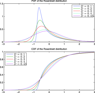
Figure 1: Plots of the PDF and CDF of $Z_{D}$ for various $D$. The CDF with the steepest slope and the PDF with the highest mode correspond to $D=0.1$.

References

- [1] {barticle}[mr] \bauthor\bsnmAbate, \bfnmJoseph\binitsJ. &\bauthor\bsnmWhitt, \bfnmWard\binitsW. (\byear1992). \btitleThe Fourier-series method for inverting transforms of probability distributions. \bjournalQueueing Systems Theory Appl. \bvolume10 \bpages5–87. \biddoi=10.1007/BF01158520, issn=0257-0130, mr=1149995 \bptokimsref \endbibitem
- [2] {bbook}[mr] \bauthor\bsnmAhues, \bfnmMario\binitsM., \bauthor\bsnmLargillier, \bfnmAlain\binitsA. &\bauthor\bsnmLimaye, \bfnmBalmohan V.\binitsB.V. (\byear2001). \btitleSpectral Computations for Bounded Operators. \bseriesApplied Mathematics (Boca Raton) \bvolume18. \baddressBoca Raton, FL: \bpublisherChapman & Hall/CRC. \biddoi=10.1201/9781420035827, mr=1886113 \bptokimsref \endbibitem
- [3] {barticle}[mr] \bauthor\bsnmAlbin, \bfnmJ. M. P.\binitsJ.M.P. (\byear1998). \btitleA note on Rosenblatt distributions. \bjournalStatist. Probab. Lett. \bvolume40 \bpages83–91. \biddoi=10.1016/S0167-7152(98)00109-6, issn=0167-7152, mr=1650532 \bptokimsref \endbibitem
- [4] {bbook}[mr] \bauthor\bsnmApplebaum, \bfnmDavid\binitsD. (\byear2004). \btitleLévy Processes and Stochastic Calculus. \bseriesCambridge Studies in Advanced Mathematics \bvolume93. \baddressCambridge: \bpublisherCambridge Univ. Press. \biddoi=10.1017/CBO9780511755323, mr=2072890 \bptokimsref \endbibitem
- [5] {bbook}[mr] \bauthor\bsnmAtkinson, \bfnmKendall\binitsK. &\bauthor\bsnmHan, \bfnmWeimin\binitsW. (\byear2009). \btitleTheoretical Numerical Analysis: A Functional Analysis Framework, \bedition3rd ed. \bseriesTexts in Applied Mathematics \bvolume39. \baddressDordrecht: \bpublisherSpringer. \bidmr=2511061 \bptokimsref \endbibitem
- [6] {barticle}[mr] \bauthor\bsnmAtkinson, \bfnmKendall E.\binitsK.E. (\byear1967). \btitleThe numerical solutions of the eigenvalue problem for compact integral operators. \bjournalTrans. Amer. Math. Soc. \bvolume129 \bpages458–465. \bidissn=0002-9947, mr=0220105 \bptokimsref \endbibitem
- [7] {barticle}[mr] \bauthor\bsnmBirman, \bfnmM. Š.\binitsM.Š. &\bauthor\bsnmSolomjak, \bfnmM. Z.\binitsM.Z. (\byear1977). \btitleEstimates for the singular numbers of integral operators. \bjournalUspehi Mat. Nauk \bvolume32 \bpages17–84, 271. \bidissn=0042-1316, mr=0438186 \bptokimsref \endbibitem
- [8] {barticle}[mr] \bauthor\bsnmBraverman, \bfnmMichael\binitsM. (\byear2005). \btitleOn a class of Lévy processes. \bjournalStatist. Probab. Lett. \bvolume75 \bpages179–189. \biddoi=10.1016/j.spl.2005.05.023, issn=0167-7152, mr=2210548 \bptokimsref \endbibitem
- [9] {barticle}[mr] \bauthor\bsnmCastaño-Martínez, \bfnmAntonia\binitsA. &\bauthor\bsnmLópez-Blázquez, \bfnmFernando\binitsF. (\byear2005). \btitleDistribution of a sum of weighted noncentral chi-square variables. \bjournalTest \bvolume14 \bpages397–415. \biddoi=10.1007/BF02595410, issn=1133-0686, mr=2211387 \bptokimsref \endbibitem
- [10] {barticle}[mr] \bauthor\bsnmChen, \bfnmZhongying\binitsZ., \bauthor\bsnmNelakanti, \bfnmGnaneshwar\binitsG., \bauthor\bsnmXu, \bfnmYuesheng\binitsY. &\bauthor\bsnmZhang, \bfnmYongdong\binitsY. (\byear2009). \btitleA fast collocation method for eigen-problems of weakly singular integral operators. \bjournalJ. Sci. Comput. \bvolume41 \bpages256–272. \biddoi=10.1007/s10915-009-9295-z, issn=0885-7474, mr=2550370 \bptokimsref \endbibitem
- [11] {barticle}[mr] \bauthor\bsnmDobrushin, \bfnmR. L.\binitsR.L. &\bauthor\bsnmMajor, \bfnmP.\binitsP. (\byear1979). \btitleNon-central limit theorems for nonlinear functionals of Gaussian fields. \bjournalZ. Wahrsch. Verw. Gebiete \bvolume50 \bpages27–52. \biddoi=10.1007/BF00535673, issn=0044-3719, mr=0550122 \bptokimsref \endbibitem
- [12] {barticle}[mr] \bauthor\bsnmDostanić, \bfnmMilutin R.\binitsM.R. (\byear1998). \btitleSpectral properties of the operator of Riesz potential type. \bjournalProc. Amer. Math. Soc. \bvolume126 \bpages2291–2297. \biddoi=10.1090/S0002-9939-98-04325-1, issn=0002-9939, mr=1451794 \bptokimsref \endbibitem
- [13] {bbook}[mr] \bauthor\bsnmGradshteyn, \bfnmI. S.\binitsI.S. &\bauthor\bsnmRyzhik, \bfnmI. M.\binitsI.M. (\byear2007). \btitleTable of Integrals, Series, and Products, \bedition7th ed. \baddressAmsterdam: \bpublisherElsevier/Academic Press. \bnoteTranslated from the Russian, Translation edited and with a preface by Alan Jeffrey and Daniel Zwillinger, With one CD-ROM (Windows, Macintosh and UNIX). \bidmr=2360010 \bptokimsref \endbibitem
- [14] {barticle}[mr] \bauthor\bsnmKac, \bfnmM.\binitsM. (\byear1955–1956). \btitleDistribution of eigenvalues of certain integral operators. \bjournalMichigan. Math. J. \bvolume3 \bpages141–148. \bidissn=0026-2285, mr=0085650 \bptokimsref \endbibitem
- [15] {bbook}[mr] \bauthor\bsnmMajor, \bfnmPéter\binitsP. (\byear1981). \btitleMultiple Wiener–Itô Integrals: With Applications to Limit Theorems. \bseriesLecture Notes in Math. \bvolume849. \baddressBerlin: \bpublisherSpringer. \bidmr=0611334 \bptokimsref \endbibitem
- [16] {bbook}[mr] \bauthor\bsnmOldham, \bfnmKeith\binitsK., \bauthor\bsnmMyland, \bfnmJan\binitsJ. &\bauthor\bsnmSpanier, \bfnmJerome\binitsJ. (\byear2009). \btitleAn Atlas of Functions, \bedition2nd ed. \baddressNew York: \bpublisherSpringer. \bnoteWith Equator, the atlas function calculator, With 1 CD-ROM (Windows). \biddoi=10.1007/978-0-387-48807-3, mr=2466333 \bptokimsref \endbibitem
- [17] {bbook}[mr] \bauthor\bsnmPeccati, \bfnmGiovanni\binitsG. &\bauthor\bsnmTaqqu, \bfnmMurad S.\binitsM.S. (\byear2011). \btitleWiener Chaos: Moments, Cumulants and Diagrams: A Survey with Computer Implementation. \bseriesBocconi & Springer Series \bvolume1. \baddressMilan: \bpublisherSpringer. \bnoteSupplementary material available online. \bidmr=2791919 \bptnotecheck year \bptokimsref \endbibitem
- [18] {bbook}[mr] \bauthor\bsnmPitman, \bfnmJ.\binitsJ. (\byear2006). \btitleCombinatorial Stochastic Processes. \bseriesLecture Notes in Math. \bvolume1875. \baddressBerlin: \bpublisherSpringer. \bnoteLectures from the 32nd Summer School on Probability Theory held in Saint-Flour, July 7–24, 2002, With a foreword by Jean Picard. \bidmr=2245368 \bptokimsref \endbibitem
- [19] {bincollection}[mr] \bauthor\bsnmRosenblatt, \bfnmM.\binitsM. (\byear1961). \btitleIndependence and dependence. In \bbooktitleProc. 4th Berkeley Sympos. Math. Statist. and Prob., Vol. II \bpages431–443. \baddressBerkeley, CA: \bpublisherUniv. California Press. \bidmr=0133863 \bptokimsref \endbibitem
- [20] {barticle}[mr] \bauthor\bsnmRosenblatt, \bfnmM.\binitsM. (\byear1963). \btitleSome results on the asymptotic behavior of eigenvalues for a class of integral equations with translation kernels. \bjournalJ. Math. Mech. \bvolume12 \bpages619–628. \bidmr=0150551 \bptokimsref \endbibitem
- [21] {bbook}[mr] \bauthor\bsnmSato, \bfnmKen-iti\binitsK.i. (\byear1999). \btitleLévy Processes and Infinitely Divisible Distributions. \bseriesCambridge Studies in Advanced Mathematics \bvolume68. \baddressCambridge: \bpublisherCambridge Univ. Press. \bnoteTranslated from the 1990 Japanese original, Revised by the author. \bidmr=1739520 \bptokimsref \endbibitem
- [22] {barticle}[mr] \bauthor\bsnmShevtsova, \bfnmI. G.\binitsI.G. (\byear2006). \btitleSharpening the upper bound for the absolute constant in the Berry–Esseen inequality. \bjournalTeor. Veroyatn. Primen. \bvolume51 \bpages622–626. \biddoi=10.1137/S0040585X97982591, issn=0040-361X, mr=2325552 \bptokimsref \endbibitem
- [23] {barticle}[mr] \bauthor\bsnmSloan, \bfnmIan H.\binitsI.H. (\byear1976). \btitleIterated Galerkin method for eigenvalue problems. \bjournalSIAM J. Numer. Anal. \bvolume13 \bpages753–760. \bidissn=0036-1429, mr=0428707 \bptokimsref \endbibitem
- [24] {barticle}[mr] \bauthor\bsnmSmith, \bfnmPeter J.\binitsP.J. (\byear1995). \btitleA recursive formulation of the old problem of obtaining moments from cumulants and vice versa. \bjournalAmer. Statist. \bvolume49 \bpages217–218. \biddoi=10.2307/2684642, issn=0003-1305, mr=1347727 \bptokimsref \endbibitem
- [25] {barticle}[mr] \bauthor\bsnmSpence, \bfnmAlastair\binitsA. (\byear1975/76). \btitleOn the convergence of the Nyström method for the integral equation eigenvalue problem. \bjournalNumer. Math. \bvolume25 \bpages57–66. \bidissn=0029-599X, mr=0395278 \bptnotecheck year \bptokimsref \endbibitem
- [26] {barticle}[mr] \bauthor\bsnmSpence, \bfnmAlastair\binitsA. (\byear1977/78). \btitleError bounds and estimates for eigenvalues of integral equations. \bjournalNumer. Math. \bvolume29 \bpages133–147. \bidissn=0029-599X, mr=0659480 \bptnotecheck year \bptokimsref \endbibitem
- [27] {bbook}[mr] \bauthor\bsnmStade, \bfnmEric\binitsE. (\byear2005). \btitleFourier Analysis. \bseriesPure and Applied Mathematics (New York). \baddressHoboken, NJ: \bpublisherWiley-Interscience. \bidmr=2125315 \bptokimsref \endbibitem
- [28] {bbook}[mr] \bauthor\bsnmSteutel, \bfnmFred W.\binitsF.W. &\bauthor\bparticlevan \bsnmHarn, \bfnmKlaas\binitsK. (\byear2004). \btitleInfinite Divisibility of Probability Distributions on the Real Line. \bseriesMonographs and Textbooks in Pure and Applied Mathematics \bvolume259. \baddressNew York: \bpublisherDekker. \bidmr=2011862 \bptokimsref \endbibitem
- [29] {barticle}[mr] \bauthor\bsnmTaqqu, \bfnmMurad S.\binitsM.S. (\byear1974/75). \btitleWeak convergence to fractional Brownian motion and to the Rosenblatt process. \bjournalZ. Wahrsch. Verw. Gebiete \bvolume31 \bpages287–302. \bidmr=0400329 \bptokimsref \endbibitem
- [30] {barticle}[mr] \bauthor\bsnmTaqqu, \bfnmMurad S.\binitsM.S. (\byear1979). \btitleConvergence of integrated processes of arbitrary Hermite rank. \bjournalZ. Wahrsch. Verw. Gebiete \bvolume50 \bpages53–83. \biddoi=10.1007/BF00535674, issn=0044-3719, mr=0550123 \bptokimsref \endbibitem
- [31] {bincollection}[auto:STB—2012/03/21—07:41:58] \bauthor\bsnmTaqqu, \bfnmM. S.\binitsM.S. (\byear2011). \btitleThe Rosenblatt process. In \bbooktitleSelected Works of Murray Rosenblatt (\beditor\bfnmRichard\binitsR. \bsnmDavis, \beditor\bfnmKeh-Shin\binitsK.S. \bsnmLii &\beditor\bfnmDimitris\binitsD. \bsnmPolitis, eds.). \baddressNew York: \bpublisherSpringer. \bptokimsref \endbibitem
- [32] {barticle}[mr] \bauthor\bsnmTudor, \bfnmCiprian A.\binitsC.A. (\byear2008). \btitleAnalysis of the Rosenblatt process. \bjournalESAIM Probab. Stat. \bvolume12 \bpages230–257. \biddoi=10.1051/ps:2007037, issn=1292-8100, mr=2374640 \bptokimsref \endbibitem
- [33] {bmisc}[auto:STB—2012/03/21—07:41:58] \bauthor\bsnmVeillette, \bfnmM. S.\binitsM.S. &\bauthor\bsnmTaqqu, \bfnmM. S.\binitsM.S. (\byear2010). \bhowpublishedBerry–Esseen and Edgeworth approximations for the tail of an infinite sum of weighted gamma random variables. Stochastic Process. Appl. To appear. Preprint available online at http://arxiv.org/abs/1010.3948. \bptokimsref \endbibitem
- [34] {barticle}[mr] \bauthor\bsnmVeillette, \bfnmMark S.\binitsM.S. &\bauthor\bsnmTaqqu, \bfnmMurad S.\binitsM.S. (\byear2011). \btitleA technique for computing the PDFs and CDFs of nonnegative infinitely divisible random variables. \bjournalJ. Appl. Probab. \bvolume48 \bpages217–237. \biddoi=10.1239/jap/1300198146, issn=0021-9002, mr=2809897 \bptokimsref \endbibitem
- [35] {bmisc}[auto:STB—2012/03/21—07:41:58] \bauthor\bsnmVeillette, \bfnmM. S.\binitsM.S. &\bauthor\bsnmTaqqu, \bfnmM. S.\binitsM.S. (\byear2012). \bhowpublishedSupplement to “Properties and numerical evaluation of the Rosenblatt distribution.” DOI:\doiurl10.3150/12-BEJ421SUPP. \bptokimsref \endbibitem
- [36] {bbook}[mr] \bauthor\bsnmZemanian, \bfnmA. H.\binitsA.H. (\byear1987). \btitleDistribution Theory and Transform Analysis: An Introduction to Generalized Functions, with Applications, \bedition2nd ed. \baddressNew York: \bpublisherDover. \bidmr=0918977 \bptokimsref \endbibitem