The Cosmology of Interacting Spin-2 Fields

Abstract

We investigate the cosmology of interacting spin-2 particles, formulating the multi-gravitational theory in terms of vierbeins and without imposing any Deser-van Nieuwen-huizen-like constraint. The resulting multi-vierbein theory represents a wider class of gravitational theories if compared to the corresponding multi-metric models. Moreover, as opposed to its metric counterpart which in general seems to contain ghosts, it has already been proved to be ghost-free. We outline a discussion about the possible matter couplings and we focus on the study of cosmological scenarios in the case of three and four interacting vierbeins. We find rich behavior, including de Sitter solutions with an effective cosmological constant arising from the multi-vierbein interaction, dark-energy solutions and nonsingular bouncing behavior.

1 Introduction

The formulation of a consistent theory of interacting spin-2 field, as a well-defined theoretical problem, has a long history [1]. These constructions in general suffer from the same Boulware-Deser ghost instability [2] that plagues non-linear extensions of massive gravity, since one can show that not only they allow but they indeed demand for at least one massive spin-2 field [3]. Recently a consistent way to suitably choose the (self)interacting terms in order to raise the cutoff of the effective theory and systematically remove the Boulware-Deser (BD) ghost for the case of one massive spin-2 field was found [4, 5]. Therefore, one could follow the same procedure in order to cure the BD instabilities for the case of two-gravity theories too [6, 7, 8].

The advantage of these non-linearly completed “bi-metric” theories is that they allow for consistent cosmological solutions in agreement with observations [9, 10, 11, 12, 13, 14, 15, 16, 17, 18, 19, 20], while their single-metric, nonlinear massive-gravity counterparts, although safe at the fundamental level, have been found to exhibit instabilities at the cosmological perturbation level [21, 22, 23, 24, 25] . Thus, it is very interesting to examine the cosmological applications of gravitational theories where more than two interacting gravitational sectors appear [37].

A crucial comment must be made at this point. Up to now, the majority of the above works in multi-gravitational theories have been performed in the metric-language, giving rise to bi-metric, tri-metric constructions etc. Although one can formulate them using the vierbeins as the fundamental fields instead, it was recently realized that the opposite is not always true, namely that the multi-vierbein constructions can be more general, without a corresponding equivalent metric formulation. For instance this is the case of the “triangle” interaction of three gravitational sectors, which although safe at the vierbein level it potentially contains ghost when formulated in terms of metrics [37].

More generally the equivalence between metric and vielbein formulations relies on a particular condition (sometime called the Deser-van Nieuwenhuizen gauge [38] for bi-metric theories) which has to be imposed on the vielbeins [39]. Although in the case of massive gravity [40], or at the perturbative level of multi-metric gravity [37], this condition arises from the field equations, in the general case of more than two interacting gravitational sectors it is not clear whether this is still true [41, 42], or if it has to be imposed as a separate assumption.

Hence, if the Deser-van Nieuwenhuizen condition is not assumed then the vielbein formulation of the theory corresponds to a different physical theory with respect to the common ghost-free bi-metric gravity. In other words, starting from the vielbein formulation of [37] without imposing any condition on the tetrads, one ends up with a theory which has no known corresponding metric formulation, and thus is in principle physically different. The un-restricted vielbein approach seems thus to describe a much wider class of theories which can be used to characterize interacting gravitational sectors. Such qualitative advantages of the vierbein formulation should be taken into account in the constructions of gravitational theories, and moreover they may enlighten the discussion of which field is the fundamental one, especially proceeding towards the quantization of the theory.

In the present work we are interested in investigating the cosmology of interacting spin-2 fields. The use of the multi-vierbein formulation allows us to incorporate interaction terms that were missed in earlier multi-metric works [49, 50, 51]. We find that even considering only extra terms which have no known metric description, it can lead to a very rich cosmology. The plan of the paper is as follows: In section 2 we present the multi-vierbein gravitational theories and in section 3 we discuss the incorporation of the matter sector. In section 4 we focus on the cosmology of three interacting spin-2 fields, extracting analytical solutions at both inflationary as well as late-times eras, while in section 5 we perform the analysis for four interacting gravitons. Finally, section 6 is devoted to the discussion and summary of the obtained results.

Notation. Greek letters are used for world (manifold) indices, while $a,b,c,...$ indices are used for local (tangent space) indices. Both take values from 0 to 3 and are summed when repeated. Indices running from $i,j,k,...$ are used to number the $N$ tetrads in the theory and are not summed if repeated unless explicitly specified. A tetrad field is related to the corresponding metric through

$$g_{\mu\nu}=\eta_{ab}\,e^{a}_{\mu}\,e^{b}_{\nu}\,,$$ (1.1)

and we use the convention $\eta_{\mu\nu}=\eta_{ab}={\rm diag}(-,+,+,+)$.

2 Multi-vielbein Action and Field Equations

We now briefly present the formulation of multi-gravitational theories describing $N$ interacting spin-2 fields in 4 dimensions [37]. The corresponding action reads

$$S=\int\sum_{i}\mathcal{L}^{(i)}_{\rm EH}+\epsilon_{abcd}\sum_{i,j,k,l}\tilde{\chi}^{ijkl}\,{\bf e}_{(i)}^{a}\wedge{\bf e}_{(j)}^{b}\wedge{\bf e}_{(k)}^{c}\wedge{\bf e}_{(l)}^{d}\,,$$ (2.1)

where the Latin indices $i,j,k,l$ run from 1 to $N$ and $\tilde{\chi}^{ijkl}$ is a completely symmetric tensor of constant coefficients. The first term provides the Einstein-Hilbert Lagrangian for every tetrad, given by

$$\mathcal{L}^{(i)}_{\rm EH}=\frac{M_{i}^{2}}{4}{\bf e}_{(i)}^{a}\wedge{\bf e}_{(i)}^{b}\wedge\star{\bf R}_{ab}^{(i)}=\frac{M_{i}^{2}}{2}\det e_{(i)}\,R^{(i)}\,,$$ (2.2)

where $M_{i}$ represents the Planck mass, ${\bf R}_{ab}^{(i)}$ the Ricci tensor 2-form and $R^{(i)}$ the scalar curvature of the $i$th tetrad field, while $\star$ denotes the Hodge dual. The second term in (2.1) accounts for the interaction terms that at most contain four tetrads.

In principle we could additionally consider parity-odd interacting terms such as, for example,

$$e_{(i)}^{a}\wedge e_{(i)}^{b}\wedge e_{(j)}{}_{a}\wedge e_{(j)}{}_{b}\,.$$ (2.3)

However, since the ghost-freedom has been proven only for action (2.1) [37] and in order to keep the analysis as simple as possible, without loss of generality we will neglect parity-odd interactions in the present work. In any case, for a first cosmological application the parity-even terms of (2.1) are adequate to capture all the novel features of the theory.

In [37, 41] it has been proven that for $N=2$ (two gravitational sectors) and imposing the Deser-van Nieuwenhuizen condition

$$e_{(1)}^{a}{}_{[\mu}e_{(2)}{}_{\nu]a}=0\,,$$ (2.4)

the theory (2.1) is equivalent to the ghost-free bi-metric gravity more commonly considered in the metric formulation [7, 8]. If this condition is not imposed, then the equivalence of the two-metric with the two-vielbein formulation is not guaranteed. On the other hand, in [42] it was shown that this condition could be restricting, since it leads to two massless propagating gravitons as in two exact copies of General Relativity. As we mentioned in the Introduction, although in the case of massive gravity [40], or at the perturbative level of multi-metric gravity [37], this condition arises from the field equations themselves, in the general non-perturbative case of more than two interacting gravitational sectors it is not clear whether this is still true [41, 42], or if it has to be imposed as a separate assumption. Therefore, in the present work we prefer not to impose the Deser-van Nieuwenhuizen condition or any other constraint on the tetrad fields. Clearly, this leads to a much wider class of multi-gravitational theories, and to formulations of multi-vierbein theories with no known corresponding metric formulation, even for only two interacting vielbeins. The resulting multi-vierbein theory is not a mere re-formulation of the multi-metric constructions, but a new, richer multi-gravitational theory.

Varying action (2.1) with respect to the tetrad one-form ${\bf e}_{(i)}^{a}$ produces the field equations

$$\frac{M_{i}^{2}}{2}{\bf e}_{(i)}^{b}\wedge\star{\bf R}_{ab}^{(i)}+\epsilon_{abcd}\sum_{j,k,l}\chi^{ijkl}\,{\bf e}_{(j)}^{b}\wedge{\bf e}_{(k)}^{c}\wedge{\bf e}_{(l)}^{d}=0\,,$$ (2.5)

which can be rewritten as

$$M_{i}^{2}G_{(i)}{}^{\mu}_{\nu}=-e_{(i)\nu}^{a}e_{(i)e}^{\mu}\epsilon_{abcd}\,\epsilon^{efgh}\sum_{i,j,k}\chi^{ijkl}X_{(ij)}{}_{f}{}^{b}X_{(ik)}{}_{g}{}^{c}X_{(il)}{}_{h}{}^{d},$$ (2.6)

where $G_{(i)}{}^{\mu}_{\nu}=R_{(i)}{}_{\nu}^{\mu}-1/2\delta^{\mu}_{\nu}R_{(i)}$ is the usual Einstein tensor of the $i$th tetrad, $\chi^{ijkl}$ is a new completely symmetric tensor of coefficients directly related to $\tilde{\chi}^{ijkl}$, and we have defined the matrices

$$X_{(ij)}{}_{a}{}^{b}=e_{(i)}^{\mu}{}_{a}e_{(j)}^{b}{}_{\mu}=(e_{(j)}e_{(i)}^{-1}){}_{a}{}^{b}\,.$$ (2.7)

The details of the derivation of the field equations can be found in Appendix A.

3 Matter Coupling

In a multi-metric gravitational theory the issue arises to which metric matter fields should couple. The viable forms of the interactions between metrics are symmetric with respect to replacing one metric with another, and in principle one could consider matter fields coupling also symmetrically to all the metrics [7, 49], as it was recently realized in the bi-metric gravity [55] . We mention here that going beyond the simple one-metric-matter coupling leads to violation of the equivalence principle, and thus such generalized couplings are potentially strongly constrained by experiments, and in particular from those related to the equivalence principle violation. Due to the Vainshtein screening mechanism at play in these gravity theories, it is not yet however clear how strong the constraints will be.

However, apart from this experimental requirement, at the theoretical level such couplings are allowed, and thus it would be interesting to consider them too in the following discussion, along with the simple one-metric-matter coupling, as a first step towards understanding their implications. When considering couplings that are linear in the matter lagrangians just as in GR, it appears that by construction the system is devoid of ghosts. Technically this is due to the matter lagrangian being linear in the lapse functions of each respective metric, and thus preserving the crucial constraint nature of the equations of motions for the lapse functions. This constraint kills one progagating degree of freedom, that would otherwise become the notorious Boulware-Deser ghost. Considering more generic possible forms of the matter coupling however would introduce nonlinear dependence on the lapse functions, resulting in the loss of the constraint and thus allowing the ghost to propagate. Generalised couplings to matter was briefly discussed in [7], and further in [57] the possibility of coupling matter to the massless combination of the metrics was explored. Since then matter lagrangian is not linear in the lapse functions of the metrics, this choice for the coupling did not turn out to be viable, as expected.

In this work we will generalize the framework of multiply-coupled matter to theories with more than two gravitational sectors, and moreover, having in mind the above discussion, we will formulate it in terms of the vierbeins. As we will see, this can be done only when the gravitational fields are non minimally coupled, that is $N$ copies of non-interacting Einstein-Hilbert theories would be either physically equivalent to General Relativity or inconsistent.

Let us begin by extending the action (2.1) as

$$S=\int\sum_{i}\mathcal{L}^{(i)}_{\rm EH}+\epsilon_{abcd}\sum_{i,j,k,l}\tilde{\chi}^{ijkl}\,{\bf e}_{(i)}^{a}\wedge{\bf e}_{(j)}^{b}\wedge{\bf e}_{(k)}^{c}\wedge{\bf e}_{(l)}^{d}+\int\sum_{i}c_{i}\mathcal{L}^{(i)}_{m}(\Phi,{\bf e}_{(i)})\,,$$ (3.1)

where the sums run from $i=1$ to $i=N$ with $N$ the number of the different vierbeins in the theory. In this case, the terms

$$S^{(i)}_{\rm matter}=\int c_{i}\mathcal{L}^{(i)}_{m}(\Phi,{\bf e}_{(i)})\,,$$ (3.2)

account for the matter action, with $\Phi$ denoting the matter fields collectively, and the dimensionless coupling constants $c_{i}$ the relative strength of the coupling of each tetrad to matter. Thus, we consider the total action to include $N$ copies of the matter Lagrangian, each having the same functional form. This is $N$-times minimally coupled theory in the sense that each $i$-term separately would reduce to the standard theory.

Varying the action (3.1) with respect to each of the tetrads we obtain $N$ field equations as

$$\frac{M_{i}^{2}}{2}{\bf e}_{(i)}^{b}\wedge\star{\bf R}_{ab}^{(i)}+\epsilon_{abcd}\sum_{j,k,l}\chi^{ijkl}\,{\bf e}_{(j)}^{b}\wedge{\bf e}_{(k)}^{c}\wedge{\bf e}_{(l)}^{d}=c_{i}T_{a}^{(i)}\,,$$ (3.3)

where the energy-momentum 3-form coupled to the $i$th tetrad is defined as

$$T_{a}^{(i)}=\frac{\delta S_{\rm matter}}{\delta e^{a}_{(i)}}=\det e_{(i)}T_{a}^{(i)\mu}\epsilon_{\mu\nu\alpha\beta}\,dx^{\nu}\wedge dx^{\alpha}\wedge dx^{\beta}\,.$$ (3.4)

These field equations can be rewritten more conveniently as

$$M_{i}^{2}G_{(i)}{}^{\mu}_{\nu}+e_{(i)\nu}^{a}e_{(i)e}^{\mu}\epsilon_{abcd}\,\epsilon^{efgh}\sum_{j,k,l}\chi^{ijkl}X_{(ij)}{}_{f}{}^{b}X_{(ik)}{}_{g}{}^{c}X_{(il)}{}_{h}{}^{d}=c_{i}T^{(i)\mu}_{\phantom{(i)}\nu},\ \$$ (3.5)

which generalize (2.6). In this expression, $T^{(i)}_{\mu\nu}$ is the stress energy tensor for the $i$th tetrad defined by

$$T^{(i)\nu}_{\mu}=T^{(i)a}_{\mu}\,e_{(i)a}^{\nu}\,.$$ (3.6)

If the matter sector can be formulated in terms of metrics this energy-momentum tensor corresponds to the standard one defined in metric General Relativity, namely

$$T^{(i)}_{\mu\nu}=\frac{-2}{\sqrt{-g_{(i)}}}\frac{\delta\left(\sqrt{-g_{(i)}}\mathcal{L}_{m}^{(i)}\right)}{\delta g_{(i)}^{\mu\nu}}\,.$$ (3.7)

On the other hand the definition with tetrads is more general since it allows to incorporate fields such as spinors that cannot be coupled to gravity as naturally, or indeed at all, within the metric formulation.

Next, we rewrite equation (3.5) as

$$M_{i}^{2}G_{\mu\nu}^{(i)}+W_{\mu\nu}^{(i)}={c_{i}}T^{(i)}_{\mu\nu}\,,$$ (3.8)

where the short-hand $W_{\mu\nu}^{(i)}$ denotes the interaction terms with the other vierbeins in the field equations. At the level of field equations the new consequence of multiple matter coupling is, as expected, that the matter fields now appear as sources in all the equations.

Additionally, note that the multiple coupling affects the behavior of matter fields, too. In order to see this more transparently we consider the conservation laws. Since each Einstein tensor is covariantly conserved with respect to its covariant derivative, it follows that

$$\nabla^{\mu}_{(i)}W_{\mu\nu}^{(i)}=\nabla^{\mu}_{(i)}{c_{i}}T^{(i)}_{\mu\nu}\,.$$ (3.9)

On the other hand, as the total matter sector should be diffeomorphism invariant, it obeys, as a whole, the conservation law

$$\sum_{i}\det e_{(i)}\nabla^{\mu}_{(i)}{c_{i}}T^{(i)}_{\mu\nu}=0\,.$$ (3.10)

Therefore, from the two separate conservation equations (3.9),(3.10), we obtain the constraint

$$\sum_{i}\frac{1}{\det e_{(i)}}\nabla^{\mu}_{(i)}W^{(i)}_{\mu\nu}=0\,.$$ (3.11)

Hence, despite the fact that the $W$-tensors are now not separately conserved, the system is consistent, and the field equations just imply that the sum (3.11) vanishes. Note that in the case where the matter fields are coupled to only one tetrad, this becomes a stronger set of $N$ constraints, $\nabla^{\mu}_{(i)}W^{(i)}_{\mu\nu}=0$, and then clearly particles would follow the geodesics of the one tetrad/metric they are coupled to. On the other hand, in the case of $N$ pure Einstein-Hilbert theories, that is when one sets the $W$-tensors to zero, equation (3.9) would force all matter to follow the geodesics of all the metrics simultaneously. In that case the metrics/tetrads would coincide with each other, and effectively the theory would reduce to General Relativity.

In general, expression (3.9) seems to imply that matter does not follow the geodesics of any tetrad. From the viewpoint of any given metric/tetrad, the multiply-coupled theory predicts violations of the equivalence principle. One expects that this fact could be used to impose strong constraints on the coupling constants $c_{i}$. The equations of motion for matter fields must be consistent with the conservation law (3.9) and they will thus involve couplings in principle to all tetrads $i$ for which $c_{i}\neq 0$.

As a concrete example, as a matter Lagrangian we consider the Lagrangian of a canonical scalar field $\phi$:

$$\mathcal{L}_{\phi}\equiv\sum_{i}c_{i}\mathcal{L}_{\phi}^{(i)}=\sum_{i}c_{i}\left[\frac{1}{2}g_{(i)}^{\mu\nu}\phi_{,\mu}\phi_{,\nu}-V(\phi)\right]\,,$$ (3.12)

where the $i$th metric is obviously given by

$$g^{\mu\nu}_{(i)}=\eta^{ab}\,e_{(i)a}^{\mu}\,e_{(i)b}^{\nu}\,.$$ (3.13)

The equations of motion can be derived by the usual Euler-Lagrange method by varying the action with respect to the scalar field, and we find

$$\sum_{i}c_{i}\det e_{(i)}\left[\Box^{(i)}\phi-V^{\prime}(\phi)\right]=0\,,$$ (3.14)

where $\Box^{(i)}$ is the dAlembertian operator of the metric $g_{(i)}$. On the other hand, inserting the Lagrangian (3.12) into the stress-energy tensor (3.7) and then into the conservation laws (3.9),(3.10),(3.11), we obtain

$$\sum_{i}\det e_{(i)}\nabla^{\mu}_{(i)}{c_{i}}T^{(i)}_{\mu\nu}=\sum_{i}c_{i}\det e_{(i)}\left[\Box^{(i)}\phi-V^{\prime}(\phi)\right]\phi_{,\nu}=0\,.$$ (3.15)

Thus, the conservation laws are guaranteed to hold due to the generalized Klein-Gordon equation (3.14) for the scalar field and do not introduce any new constraint. In summary, we have thus seen how the multiple coupling consistently modifies both the structure of the gravitational equations and the equations of motion for the matter fields.

Finally, we mention that the case of two metrics coupled to dust-like matter in cosmological spacetimes was investigated in detail in [55], and it was found that each term in the sums (3.10) and (3.11) vanishes independently. Thus, it remains to be seen how this features generally occurs, and how stringent are the constraints ensuing from the violations of the usual conservation laws when it does not occur.

4 Three-Vierbein Cosmology

Let us now investigate the cosmological applications of the multi-vierbein gravity formulated above. In this section we focus on three interacting tetrads, while in the next one we will study the four interacting vierbein scenario. Assuming three interacting gravitational sectors, that is setting $N=3$ in the expressions of the previous section, we result in 15 coupling terms in four dimensions, namely: 3 cosmological constant terms ($\Lambda_{1}$, $\Lambda_{2}$, $\Lambda_{2}$), 9 terms coupling pairs of tetrads ($\beta_{1}$, … , $\beta_{9}$) and 3 terms coupling all the three tetrads together ($\alpha_{1}$, $\alpha_{2}$, $\alpha_{3}$). The theory can be graphically visualized as in Fig. 1 (a), where the coupling parameters are associated to the corresponding edge.

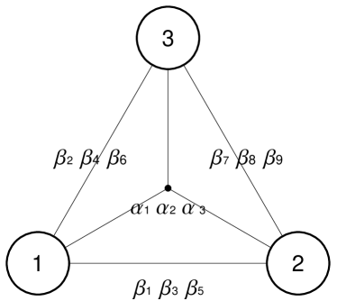
(a)

(b)

Figure 1: Graphic representation of the three-vierbein theory in four dimensions. The $\beta$-edges represent the terms coupling pair of tetrads, while the $\alpha$ three-vertex junctions represent the terms coupling three tetrads together. The $\Lambda$-terms (cosmological constants) correspond to self-interacting/closed lines and have not be drawn.

In order to investigate the cosmological evolution in a universe governed by the three-interacting spin-2 field theory, we assume that the three tetrads take the form

$$e_{(1)}{}_{\mu}^{a}=\mbox{diag}\left(N_{a}(t),\frac{a(t)}{\sqrt{1-k\,r^{2}}},a(t)\,r,a(t)\,r\,\sin\theta\right)$$

$$e_{(2)}{}_{\mu}^{a}=\mbox{diag}\left(N_{b}(t),\frac{b(t)}{\sqrt{1-k\,r^{2}}},b(t)\,r,b(t)\,r\,\sin\theta\right)$$

$$e_{(3)}{}_{\mu}^{a}=\mbox{diag}\left(N_{c}(t),\frac{c(t)}{\sqrt{1-k\,r^{2}}},c(t)\,r,c(t)\,r\,\sin\theta\right),\ \ \ \ \$$ (4.1)

corresponding to the three Friedmann-Robertson-Walker (FRW) metrics

$$ds^{2}_{1}=-N_{a}(t)^{2}\,dt^{2}+a(t)^{2}\left(\frac{dr^{2}}{1-kr^{2}}+r^{2}d\Omega^{2}\right)$$

$$ds^{2}_{2}=-N_{b}(t)^{2}\,dt^{2}+b(t)^{2}\left(\frac{dr^{2}}{1-kr^{2}}+r^{2}d\Omega^{2}\right)$$

$$ds^{2}_{3}=-N_{c}(t)^{2}\,dt^{2}+c(t)^{2}\left(\frac{dr^{2}}{1-kr^{2}}+r^{2}d\Omega^{2}\right),$$ (4.2)

where $N_{a}$, $N_{b}$, $N_{c}$, $a$, $b$, $c$ (the three lapse functions and the three scale factors) are all functions of $t$, $k=0,\pm 1$ as usual and $d\Omega^{2}=d\theta^{2}+\sin^{2}\theta\,d\phi^{2}$ is the 2-sphere line element. Note that, similarly to the bi-metric gravity case, we are considering that the spatial curvature of all the three metrics is the same. If this assumption is relaxed then inconsistencies arise from the field equations, similarly to the bi-metric gravity case [21, 22, 23, 24, 25]. Furthermore, although as usual we could eliminate one lapse function redefining the time $t$, for clarity and generality we keep all the $N_{i}$ in the forthcoming expressions, having in mind that one of them can be set to unity at any moment.

We mention here that the FRW assumptions for the tetrads indeed solve the Deser-van Nieuwenhizen condition (2.4). This means that even though the theory we are dealing with does not contain such condition in general, at the cosmological level such restriction is automatically satisfied. As a consequence, all the results we will find in this and the following sections will hold also in the corresponding metric description of the theory.

Finally, a comment should be made concerning the vierbein choice corresponding to a specific metric. As it is known, due to the local Lorentz invariance there are infinite vierbein choices producing a given metric. Since in the multi-vierbein gravity of action (2.1) the interacting terms do not involve derivatives of the tetrads, one can straightforwardly verify that it is local Lorentz invariant and thus any Lorentz-transformed, non-diagonal, vierbein choice would lead to the same field equations. Therefore, in this work we consider diagonal vierbeins for simplicity and without loss of generality. However, note that this is not a priori possible in any modified gravitational theory, since in the case where local Lorentz invariance is broken the vierbeins should be chosen very carefully (for instance in the case of $f(T)$ gravity [58, 59]).

4.1 Vacuum solutions

Let us first investigate the vacuum solutions of the theory, that is we consider the field equations (2.6) without the matter sector of section 3. Inserting the tetrads (4.1) inside the field equations (2.6) yields the following three first Friedmann equations

$$3M_{1}^{2}\left(\frac{k}{a^{2}}+\frac{H_{a}^{2}}{N_{a}^{2}}\right)=\Lambda_{1}+3\beta_{1}\frac{b}{a}+3\beta_{2}\frac{c}{a}+3\beta_{3}\frac{b^{2}}{a^{2}}$$

$$\ \ \ +3\beta_{4}\frac{c^{2}}{a^{2}}+\beta_{5}\frac{b^{3}}{a^{3}}+\beta_{6}\frac{c^{3}}{a^{3}}+2\alpha_{1}\frac{bc}{a^{2}}+\alpha_{2}\frac{b^{2}c}{a^{3}}+\alpha_{3}\frac{bc^{2}}{a^{3}},$$

$$3M_{2}^{2}\left(\frac{k}{b^{2}}+\frac{H_{b}^{2}}{N_{b}^{2}}\right)=\Lambda_{2}+\beta_{1}\frac{a^{3}}{b^{3}}+3\beta_{3}\frac{a^{2}}{b^{2}}+3\beta_{5}\frac{a}{b}$$

$$\ \ \ +3\beta_{7}\frac{c}{b}+3\beta_{8}\frac{c^{2}}{b^{2}}+\beta_{9}\frac{c^{3}}{b^{3}}+\alpha_{1}\frac{a^{2}c}{b^{3}}+2\alpha_{2}\frac{ac}{b^{2}}+\alpha_{3}\frac{ac^{2}}{b^{3}},$$

$$3M_{3}^{2}\left(\frac{k}{c^{2}}+\frac{H_{c}^{2}}{N_{c}^{2}}\right)=\Lambda_{3}+\beta_{2}\frac{a^{3}}{c^{3}}+3\beta_{4}\frac{a^{2}}{c^{2}}+3\beta_{6}\frac{3a}{c}\$$

$$\ +\beta_{7}\frac{b^{3}}{c^{3}}+3\beta_{8}\frac{b^{2}}{c^{2}}+3\beta_{9}\frac{b}{c}\alpha_{1}\frac{a^{2}b}{c^{3}}+\alpha_{2}\frac{ab^{2}}{c^{3}}+2\alpha_{3}\frac{ab}{c^{2}},\ \$$ (4.3)

plus the three acceleration equations

$$\frac{M_{1}^{2}}{N_{a}^{2}}\left(N_{a}^{2}\frac{k}{a^{2}}+2\dot{H}_{a}+3H_{a}^{2}-2H_{a}\frac{\dot{N}_{a}}{N_{a}}\right)=\ \ \ \$$

$$\ \ \Lambda_{1}+\beta_{1}\left(2\frac{b}{a}+\frac{N_{b}}{N_{a}}\right)+\beta_{2}\left(2\frac{c}{a}+\frac{N_{c}}{N_{a}}\right)$$

$$\ \ +\beta_{3}\left(\frac{b^{2}}{a^{2}}+2\frac{bN_{b}}{aN_{a}}\right)+\beta_{4}\left(\frac{c^{2}}{a^{2}}+2\frac{cN_{c}}{aN_{a}}\right)$$

$$\ \ +\beta_{5}\frac{b^{2}N_{b}}{a^{2}N_{a}}+\beta_{6}\frac{c^{2}N_{c}}{a^{2}N_{a}}$$

$$\ \ +\frac{2\alpha_{1}}{3}\left(\frac{bc}{a^{2}}+\frac{bN_{c}}{aN_{a}}+\frac{cN_{b}}{aN_{a}}\right)+\frac{\alpha_{2}}{3}\left(\frac{b^{2}N_{c}}{a^{2}N_{a}}+2\frac{bcN_{b}}{a^{2}N_{a}}\right)$$

$$\ \ +\frac{\alpha_{3}}{3}\left(\frac{c^{2}N_{b}}{a^{2}N_{a}}+2\frac{bcN_{c}}{a^{2}N_{a}}\right),\ \$$ (4.4)

$$\frac{M_{2}^{2}}{N_{b}^{2}}\left(N_{b}^{2}\frac{k}{b^{2}}+2\dot{H}_{b}+3H_{b}^{2}-2H_{b}\frac{\dot{N}_{b}}{N_{b}}\right)=\ \ \ \$$

$$\ \ \Lambda_{2}+\beta_{1}\frac{a^{2}N_{a}}{b^{2}N_{b}}+\beta_{3}\left(\frac{a^{2}}{b^{2}}+2\frac{aN_{a}}{bN_{b}}\right)$$

$$\ \ +\beta_{5}\left(2\frac{a}{b}+\frac{N_{a}}{N_{b}}\right)+\beta_{7}\left(2\frac{c}{b}+\frac{N_{c}}{N_{b}}\right)$$

$$\ \ +\beta_{8}\left(\frac{c^{2}}{b^{2}}+2\frac{cN_{c}}{bN_{b}}\right)+\beta_{9}\frac{c^{2}N_{c}}{b^{2}N_{b}}$$

$$\ \ +\frac{\alpha_{1}}{3}\left(\frac{a^{2}N_{c}}{b^{2}N_{b}}+2\frac{acN_{a}}{b^{2}N_{b}}\right)+\frac{2\alpha_{2}}{3}\left(\frac{ac}{b^{2}}+\frac{aN_{c}}{bN_{b}}+\frac{cN_{a}}{bN_{b}}\right)$$

$$\ \ +\frac{\alpha_{3}}{3}\left(\frac{c^{2}N_{a}}{b^{2}N_{b}}+2\frac{acN_{c}}{b^{2}N_{b}}\right),$$ (4.5)

$$\frac{M_{3}^{2}}{N_{c}^{2}}\left(N_{c}^{2}\frac{k}{c^{2}}+2\dot{H}_{c}+3H_{c}^{2}-2H_{c}\frac{\dot{N}_{c}}{N_{c}}\right)=\ \ \ \$$

$$\ \ \Lambda_{3}+\beta_{2}\frac{a^{2}N_{a}}{c^{2}N_{c}}+\beta_{4}\left(\frac{a^{2}}{c^{2}}+2\frac{aN_{a}}{cN_{c}}\right)+\beta_{6}\left(2\frac{a}{c}+\frac{N_{a}}{N_{c}}\right)$$

$$\ \ +\beta_{7}\frac{b^{2}N_{b}}{c^{2}N_{c}}+\beta_{8}\left(\frac{b^{2}}{c^{2}}+2\frac{bN_{b}}{cN_{c}}\right)+\beta_{9}\left(2\frac{b}{c}+\frac{N_{b}}{N_{c}}\right)$$

$$\ \ +\frac{\alpha_{1}}{3}\left(\frac{a^{2}N_{b}}{c^{2}N_{c}}+2\frac{abN_{a}}{c^{2}N_{c}}\right)+\frac{\alpha_{2}}{3}\left(\frac{b^{2}N_{a}}{c^{2}N_{c}}+2\frac{abN_{b}}{c^{2}N_{c}}\right)$$

$$\ \ +\frac{2\alpha_{3}}{3}\left(\frac{ab}{c^{2}}+\frac{aN_{b}}{cN_{c}}+\frac{bN_{a}}{cN_{c}}\right)\,,$$ (4.6)

where $H_{a}=\dot{a}/a$, $H_{b}=\dot{b}/b$, $H_{c}=\dot{c}/c$ are the three Hubble functions and an overdot denotes differentiation with respect to $t$. The parameters appearing in (4.1)-(4.6) are related to the completely symmetric tensor of coefficients $\chi^{ijkl}$ of equation (2.5) through

$$\Lambda_{1}=6\,\chi^{1111}\,,\quad\Lambda_{2}=6\,\chi^{2222}\,,\quad\Lambda_{3}=6\,\chi^{3333}\,,$$

$$\beta_{1}=6\,\chi^{1112}\,,\quad\beta_{2}=6\,\chi^{1113}\,,\quad\beta_{3}=6\,\chi^{1122}\,,$$

$$\beta_{4}=6\,\chi^{1133}\,,\quad\beta_{5}=6\,\chi^{1222}\,,\quad\beta_{6}=6\,\chi^{1333}\,,$$

$$\beta_{7}=6\,\chi^{2223}\,,\quad\beta_{8}=6\,\chi^{2233}\,,\quad\beta_{9}=6\,\chi^{2333}\,,$$

$$\alpha_{1}=18\,\chi^{1123}\,,\quad\alpha_{2}=18\,\chi^{1223}\,,\quad\alpha_{3}=18\,\chi^{1233}\,.$$ (4.7)

From these expressions we deduce that the $\Lambda_{i}$ are just the cosmological constants for the three vierbeins and do not couple different fields, the $\beta$-terms couple pair of fields, and finally the $\alpha$-terms acount for the “triangular” interactions of all the three vierbeins, as was conveniently visualized in Fig. 1 (a).

As we discussed in the Introduction, the $\alpha$-terms, which are the fully interacting ones, do not have a known metric corresponding description, especially if we do not apply the Deser-van Nieuwenhuizen condition or any other constraint on the tetrad fields. That is why although the simple interacting $\beta$ and $\Lambda$ terms were considered in [49] within a metric formulation of the theory, the full interaction was necessarily neglected.

In this work we are interested in exactly these full interacting terms, and in the novel features they bring to cosmology. Thus, we focus on a theory where only the $\alpha$-terms are non vanishing, that is to the model depicted in Fig. 1 (b). Obviously, one can straightforwardly study the full theory too.

With these assumptions the Friedmann equations (4.3) read

$$3M_{1}^{2}\left(\frac{k}{a^{2}}+\frac{H_{a}^{2}}{N_{a}^{2}}\right)=2\alpha_{1}\frac{bc}{a^{2}}+\alpha_{2}\frac{b^{2}c}{a^{3}}+\alpha_{3}\frac{bc^{2}}{a^{3}},$$

$$3M_{2}^{2}\left(\frac{k}{b^{2}}+\frac{H_{b}^{2}}{N_{b}^{2}}\right)=\alpha_{1}\frac{a^{2}c}{b^{3}}+2\alpha_{2}\frac{ac}{b^{2}}+\alpha_{3}\frac{ac^{2}}{b^{3}},$$

$$3M_{3}^{2}\left(\frac{k}{c^{2}}+\frac{H_{c}^{2}}{N_{c}^{2}}\right)=\alpha_{1}\frac{a^{2}b}{c^{3}}+\alpha_{2}\frac{ab^{2}}{c^{3}}+2\alpha_{3}\frac{ab}{c^{2}}\,,\$$ (4.8)

and the acceleration equations (4.4)-(4.6) reduce to

$$\frac{M_{1}^{2}}{N_{a}^{2}}\left(N_{a}^{2}\frac{k}{a^{2}}+2\dot{H}_{a}+3H_{a}^{2}-2H_{a}\frac{\dot{N}_{a}}{N_{a}}\right)=\ \ \ \$$

$$\ \ \frac{2\alpha_{1}}{3}\left(\frac{bc}{a^{2}}+\frac{bN_{c}}{aN_{a}}+\frac{cN_{b}}{aN_{a}}\right)+\frac{\alpha_{2}}{3}\left(\frac{b^{2}N_{c}}{a^{2}N_{a}}+2\frac{bcN_{b}}{a^{2}N_{a}}\right)$$

$$+\frac{\alpha_{3}}{3}\left(\frac{c^{2}N_{b}}{a^{2}N_{a}}+2\frac{bcN_{c}}{a^{2}N_{a}}\right),$$ (4.9)

$$\frac{M_{2}^{2}}{N_{b}^{2}}\left(N_{b}^{2}\frac{k}{b^{2}}+2\dot{H}_{b}+3H_{b}^{2}-2H_{b}\frac{\dot{N}_{b}}{N_{b}}\right)=\ \ \ \$$

$$\ \ \frac{\alpha_{1}}{3}\left(\frac{a^{2}N_{c}}{b^{2}N_{b}}+2\frac{acN_{a}}{b^{2}N_{b}}\right)+\frac{2\alpha_{2}}{3}\left(\frac{ac}{b^{2}}+\frac{aN_{c}}{bN_{b}}+\frac{cN_{a}}{bN_{b}}\right)$$

$$+\frac{\alpha_{3}}{3}\left(\frac{c^{2}N_{a}}{b^{2}N_{b}}+2\frac{acN_{c}}{b^{2}N_{b}}\right),$$ (4.10)

$$\frac{M_{3}^{2}}{N_{c}^{2}}\left(N_{c}^{2}\frac{k}{c^{2}}+2\dot{H}_{c}+3H_{c}^{2}-2H_{c}\frac{\dot{N}_{c}}{N_{c}}\right)=\ \ \ \$$

$$\ \ \frac{\alpha_{1}}{3}\left(\frac{a^{2}N_{b}}{c^{2}N_{c}}+2\frac{abN_{a}}{c^{2}N_{c}}\right)+\frac{\alpha_{2}}{3}\left(\frac{b^{2}N_{a}}{c^{2}N_{c}}+2\frac{abN_{b}}{c^{2}N_{c}}\right)$$

$$+\frac{2\alpha_{3}}{3}\left(\frac{ab}{c^{2}}+\frac{aN_{b}}{cN_{c}}+\frac{bN_{a}}{cN_{c}}\right)\,.$$ (4.11)

In the following subsections we extract analytical solutions of the above equations.

4.1.1 Analytic Solutions: General Considerations

In order to solve the cosmological equations (4.8)-(4.1) it proves more convenient to impose specific ansätze. Firstly, we reparametrize the time $t$ setting $N_{a}=1$. Additionally, we set

$$N_{b}=\frac{\dot{b}}{\dot{a}}\quad\mbox{and}\quad N_{c}=\frac{\dot{c}}{\dot{a}}\,,$$ (4.12)

which directly generalize the usual assumption one makes in bi-metric gravity in order to satisfy the Bianchi constraint (3.11). In particular, substituting the functions (4.12) inside the Bianchi constraint (3.11) leads to an automatic satisfaction, that is these ansätze are a good starting point for our theory too. Finally, it proves convenient to define

$$\mathcal{B}=\frac{b}{a}\quad\mbox{and}\quad\mathcal{C}=\frac{c}{a}.$$ (4.13)

Thus, the first Friedmann equations (4.8) reduce to

$$3M_{1}^{2}\left(\frac{k}{a^{2}}+H_{a}^{2}\right) =2\alpha_{1}\mathcal{B}\mathcal{C}+\alpha_{2}\mathcal{B}^{2}\mathcal{C}+\alpha_{3}\mathcal{B}\mathcal{C}^{2}\,,$$ (4.14)

$$3M_{2}^{2}\left(\frac{k}{a^{2}}+H_{a}^{2}\right) =\alpha_{1}\frac{\mathcal{C}}{\mathcal{B}}+2\alpha_{2}\mathcal{C}+\alpha_{3}\frac{\mathcal{C}^{2}}{\mathcal{B}}\,,$$ (4.15)

$$3M_{3}^{2}\left(\frac{k}{a^{2}}+H_{a}^{2}\right) =\alpha_{1}\frac{\mathcal{B}}{\mathcal{C}}+\alpha_{2}\frac{\mathcal{B}^{2}}{\mathcal{C}}+2\alpha_{3}\mathcal{B}\,.$$ (4.16)

Subtraction of these equations eliminates the left-hand sides, and then we can furthermore eliminate $\mathcal{B}$, obtaining a polynomial equation for $\mathcal{C}$, which in general is of seventh order. If $\mathcal{C}\neq M_{1}/M_{3}$, which is true in general, this equation writes as

$$z_{0}+z_{1}\mathcal{C}+z_{2}\mathcal{C}^{2}+z_{3}\mathcal{C}^{3}+z_{4}\mathcal{C}^{4}+z_{5}\mathcal{C}^{5}+z_{6}\mathcal{C}^{6}+z_{7}\mathcal{C}^{7}=0\,,$$ (4.17)

with the constant coefficients given by

$$z_{0}=M_{1}^{4}\alpha_{1}\left(M_{2}^{2}\alpha_{1}^{2}+M_{1}^{2}\alpha_{2}^{2}\right)\,,$$

$$z_{1}=3\frac{\alpha_{3}}{\alpha_{1}}z_{0}\,,\qquad z_{2}=-M_{1}^{2}M_{3}^{2}\alpha_{1}\left(4M_{2}^{2}\alpha_{1}^{2}+5M_{1}^{2}\alpha_{2}^{2}\right)\,,$$

$$z_{3}=-M_{1}^{2}\alpha_{3}\left(7M_{1}^{2}M_{3}^{2}\alpha_{2}^{2}+6M_{2}^{2}M_{3}^{2}\alpha_{1}^{2}+4M_{1}^{2}M_{2}^{2}\alpha_{3}^{2}\right)\,,$$

$$z_{4}=M_{3}^{2}\alpha_{1}\left(7M_{1}^{2}M_{3}^{2}\alpha_{2}^{2}+4M_{2}^{2}M_{3}^{2}\alpha_{1}^{2}+6M_{1}^{2}M_{2}^{2}\alpha_{3}^{2}\right)\,,$$

$$z_{5}=M_{1}^{2}M_{3}^{2}\alpha_{3}\left(5M_{3}^{2}\alpha_{2}^{2}+4M_{2}^{2}\alpha_{3}^{2}\right)\,,$$

$$z_{6}=3\frac{\alpha_{1}}{\alpha_{3}}z_{7}\,,\qquad z_{7}=-M_{3}^{4}\alpha_{3}\left(M_{3}^{2}\alpha_{2}^{2}+M_{2}^{2}\alpha_{3}^{2}\right)\,.$$ (4.18)

The existence of a real solution for $\mathcal{C}$ of the algebraic equation (4.17) is a necessary (but not sufficient) condition for the existence of a cosmological solution. In particular, inserting $\mathcal{C}$ into (4.14)-(4.16) provides $\mathcal{B}$ and the scale factor $a$. Note that the fact that $\mathcal{C}$ and $\mathcal{B}$ are constants implies that $c\propto b\propto a$. Moreover, the acceleration equations (4.1)-(4.1) will be then automatically satisfied, since the ansätze (4.12) satisfy the Bianchi constraint (3.11) which directly follows from the field equations. Finally, we stress here that in the present three-vierbein cosmology the seventh-order equation (4.17) does not always have a real solution, while in bi-metric gravity the corresponding equation is of fourth order and always admits a real solution [10].

In general, the extraction of the solutions of (4.17) is a hard task. Since in this work we do not desire to rely on numerical elaboration, in the following subsections we focus on specific simple parameter choices which allow for analytical solutions, with however very interesting cosmological implications. Lastly, without loss of generality, in the following we assume the positivity of the Planck masses: $M_{1}>0$, $M_{2}>0$ and $M_{3}>0$.

4.1.2 Solutions with two $\alpha$’s being zero

We first examine the case where two $\alpha$’s are zero. Assuming that $\alpha_{1}=\alpha_{2}=0$, equations (4.14)-(4.17) lead straightforwardly to

$$\mathcal{B}=\frac{M_{1}}{M_{2}}\,,\quad\mbox{and}\quad\mathcal{C}=\sqrt{2}\frac{M_{1}}{M_{3}}\,.$$ (4.19)

Thus, we obtain $c\propto b\propto a$, and the expanding solution will be given by

$$a(t)=\frac{3}{2}\frac{kM_{2}M_{3}^{2}}{a_{0}}\exp\left[-\sqrt{\frac{2\alpha_{3}M_{1}}{3M_{2}}}\frac{t}{M_{3}}\right]+\frac{a_{0}}{4\alpha_{3}M_{1}}\exp\left[\sqrt{\frac{2\alpha_{3}M_{1}}{3M_{2}}}\frac{t}{M_{3}}\right]\,,$$ (4.20)

where $a_{0}$ is a constant of integration. Therefore, since the first exponential quickly becomes sub-dominant (or it is automatically zero in the case of a flat universe), this specific triangle interaction induces a standard de-Sitter universe with an effective cosmological constant

$$\Lambda_{eff}=\frac{1}{M_{3}}\sqrt{\frac{2\alpha_{3}M_{1}}{3M_{2}}},$$ (4.21)

where we have to impose $\alpha_{3}>0$ in order to have an expanding scale factor.

Now, due to symmetry, the above solution (4.20) can be obtained in the case where $\alpha_{1}=\alpha_{3}=0$, with the replacements $\alpha_{2}\leftrightarrow\alpha_{3}$ and $M_{2}\leftrightarrow M_{3}$, while instead of (4.19) we will have

$$\mathcal{B}=\sqrt{2}\frac{M_{1}}{M_{2}}\quad\mbox{and}\quad\mathcal{C}=\frac{M_{1}}{M_{3}}\,.$$ (4.22)

Again we can find a de-Sitter solution when $\alpha_{2}>0$.

Finally, we examine the case $\alpha_{2}=\alpha_{3}=0$, which in principle is theoretically different from the previous ones since we are setting to zero the interactions between the vierbeins whose time coordinate has not been normalized. However, the calculations are the same and from (4.14)-(4.16) we acquire

$$\mathcal{B}=\frac{M_{1}}{\sqrt{2}M_{2}}\quad\mbox{and}\quad\mathcal{C}=\frac{M_{1}}{\sqrt{2}M_{3}}\,,$$ (4.23)

that is $c\propto b\propto a$ and thus an effective cosmological constant in the evolution equations (4.8)-(4.1). The general expanding solution is given by

$$a(t)=\frac{3}{2}\frac{kM_{2}M_{3}}{a_{0}}\exp\left[-\sqrt{\frac{\alpha_{1}}{3M_{2}M_{3}}}t\right]+\frac{a_{0}}{2\alpha_{1}}\exp\left[\sqrt{\frac{\alpha_{1}}{3M_{2}M_{3}}}t\right]\,,$$ (4.24)

which is structurally the same as the ones obtained above, that is it describes an open or flat de-Sitter expansion when $\alpha_{1}>0$.

4.1.3 Bouncing Behavior

Interestingly, the system allows for non-singular bouncing behavior too. For instance, although in the case of a flat universe (4.20) describes an exact de Sitter solution, considering a closed universe ($k>0$) and going sufficiently back in time we obtain a cosmological bounce. This can be more transparently seen if we assume for example $\alpha_{1}=\alpha_{2}=0$, $k>0$ and choose the integration constant $a_{0}$ to be $a_{0}=\sqrt{6kM_{1}M_{2}M_{3}^{2}\alpha_{3}}$, in which case the solution (4.20) becomes

$$a(t)=\sqrt{\frac{3kM_{2}M_{3}^{2}}{2\alpha_{3}M_{1}}}\cosh{\left(\omega t\right)}\,,$$ (4.25)

with $\omega=\Lambda_{eff}$, while the Hubble rate as a function of time is

$$H(t)=\omega\tanh{\left(\omega t\right)}\,.$$ (4.26)

This solution describes a bouncing universe which is initially contracting and then turns into an expanding phase. Note that in the asymptotic past and future the universe exhibits a de Sitter behavior. Thus, this solution can model also geodesically-completed inflationary cosmologies.

Similarly to the previous paragraph, for the case $\alpha_{2}=\alpha_{3}=0$ we can also find bouncing behavior similar to (4.25). If we now choose $a_{0}=\sqrt{3kM_{2}M_{3}\alpha_{1}}$, then (4.24) can be rewritten as

$$a(t)=\sqrt{\frac{3kM_{2}M_{3}}{\alpha_{1}}}\cosh{\left(\sqrt{\frac{\alpha_{1}}{3M_{2}M_{3}}}t\right)}\,.$$ (4.27)

Moreover, note that more general classes of non-singular behaviours, in particular asymmetric bounces, are easy to be obtained by choosing different $a_{0}$. In the above example we just presented the simplest $\cosh$-solution in order to illustrate the bouncing possibility. We mention that in the present multi-vierbein theory it is possible to find non-singular solutions even in vacuum, whereas in General Relativity to avoid the Big Bang singularity requires one to introduce energy-condition-violating matter sources [65, 66]. In the following we will see that, assuming closed universe, such vacuum solutions are generic in multi-vierbein theories.

4.1.4 de-Sitter Solutions

As it is clear from the previous paragraphs, de-Sitter solutions are particularly common in this theory. This is a general feature arising whenever one sets $b$ and $c$ proportional to $a$. In this case all the interacting terms in (4.8) will become constants, inducing an overall cosmological constant for all the three equations. If we then assume spatial flatness ($k=0$) and spend our time-reparametrization invariance setting $N_{a}=1$, we will find from the first equation of (4.8) the expanding solution

$$a(t)=a_{0}\exp\left[\frac{t}{M_{1}}\sqrt{\frac{2\mathcal{B}\mathcal{C}}{3}\left(2\alpha_{1}+\mathcal{B}\alpha_{2}+\mathcal{C}\alpha_{3}\right)}\right]\,,$$ (4.28)

where we have introduced $b=\mathcal{B}\,a$ and $c=\mathcal{C}\,a$ as in (4.13). This solution corresponds to a de-Sitter universe, with the cosmological constant depending on the interacting parameters and the two constants $\mathcal{B}$ and $\mathcal{C}$. However, in order to complete the solution we must also satisfy the other cosmological equations. The remaining two Friedmann equations of (4.8) will provide solutions for the two lapse functions $N_{b}$ and $N_{c}$, which turn out to be constants depending on the free parameters of the theory. The three acceleration equations (4.1)-(4.1) transform into two algebraic relations which determine the values of $\mathcal{B}$ and $\mathcal{C}$ in terms of the theoretical parameters. Usually these equations imply a rather involved expression for these constants, but it considerably simplifies for some simple cases such as, for example, the ones considered above.

4.1.5 Solutions with $c=a\,M_{1}/M_{3}$

In order to extract equation (4.17) we assumed that $\mathcal{C}\neq M_{1}/M_{3}$. If this is not the case, that is if $\mathcal{C}=M_{1}/M_{3}$, then equations (4.14)-(4.16) are satisfied only if $\alpha_{1}M_{3}=\alpha_{3}M_{1}$, resulting to a cubic equation for $\mathcal{B}$:

$$-2\frac{\alpha_{1}}{M_{2}^{2}}+-2\frac{\alpha_{2}}{M_{2}^{2}}\mathcal{B}+3\frac{\alpha_{1}}{M_{1}^{2}}\mathcal{B}^{2}+\frac{\alpha_{2}}{M_{1}^{2}}\mathcal{B}^{3}=0.$$ (4.29)

If one of $\alpha_{1}$ or $\alpha_{3}$ is zero, then the other will be too, and thus we result in the case described in paragraph 4.1.2. However, if only $\alpha_{2}=0$ then equation (4.29) has the unique positive solution

$$\mathcal{B}=\sqrt{\frac{2}{3}}\frac{M_{1}}{M_{2}}\,,$$ (4.30)

that is $c\propto b\propto a$ which implies an effective cosmological constant in the Friedmann equations (4.8). The expanding solution will then be

$$a(t)=\frac{3}{2}\frac{kM_{2}M_{3}}{a_{0}}\exp\left[-\left(\frac{2}{3}\right)^{1/4}\sqrt{\frac{\alpha_{1}}{M_{2}M_{3}}}t\right]+\frac{a_{0}}{2\sqrt{6}\alpha_{1}}\exp\left[\left(\frac{2}{3}\right)^{1/4}\sqrt{\frac{\alpha_{1}}{M_{2}M_{3}}}t\right],\ \ \$$ (4.31)

which becomes a pure de-Sitter universe for $k=0$ and $\alpha_{1}>0$, or a late-time de Sitter universe for $k>0$ and and $\alpha_{1}>0$. Additionally, since the equations are symmetric in the vierbein exchange $2\leftrightarrow 3$, we obtain another solution similar to (4.31), with the substitutions $\alpha_{2}\leftrightarrow\alpha_{3}$ and $M_{2}\leftrightarrow M_{3}$.

Finally, note that in this case we also find non-singular bouncing evolutions. For example the choice $a_{0}=\sqrt{3k\sqrt{6}M_{2}M_{3}\alpha_{1}}$ corresponds to

$$a(t)=\sqrt{\frac{\sqrt{6}kM_{2}M_{3}}{2\alpha_{1}}}\cosh{\left[\left(\frac{2}{3}\right)^{\frac{1}{4}}\sqrt{\frac{\alpha_{1}}{M_{2}M_{3}}}t\right]}\,,$$ (4.32)

which exhibits a bounce before transiting to an expanding de Sitter universe.

We close this paragraph mentioning that all the above vacuum solutions fulfill the Friedmann equation with a constant source. Therefore, all of them correspond to the same family, that is to the de Sitter one (although under specific conditions they can exhibit a bouncing behavior before entering the pure de Sitter regime).

4.2 Matter solutions

In order to obtain a late-time description of the universe, we must take into account the matter sector. According to the discussion of section 3 the choice of the matter coupling will yield constraints on the field equations. In this section we will consider two cases in particular and we will find simple analytical solutions to the field equations.

4.2.1 Matter coupled to one (physical) vierbein

The first case we consider is when the matter sector is coupled to one tetrad only, which thus turns out to be the physical vierbein. This is the simplest and usual case, since it satisfies the equivalence principle. We assume that matter can be described by a perfect fluid with $\rho_{m}$ and $p_{m}$ its energy density and pressure respectively. The coupled/physical tetrad will be the one with the scale factor $a$, that is we set $c_{1}=1$ and $c_{2}=c_{3}=0$ in action (3.1). Focusing on the $\alpha$-terms as before, that is to the three-vertex interaction, the Friedmann equations for the physical vierbein now read as

$$3M_{1}^{2}\left(\frac{k}{a^{2}}+\frac{H_{a}^{2}}{N_{a}^{2}}\right)=\rho_{m}+2\alpha_{1}\frac{bc}{a^{2}}+\alpha_{2}\frac{b^{2}c}{a^{3}}+\alpha_{3}\frac{bc^{2}}{a^{3}},$$ (4.33)

$$\frac{M_{1}^{2}}{N_{a}^{2}}\left(N_{a}^{2}\frac{k}{a^{2}}+2\dot{H}_{a}+3H_{a}^{2}-2H_{a}\frac{\dot{N}_{a}}{N_{a}}\right)=-p_{m}+\frac{2\alpha_{1}}{3}\left(\frac{bc}{a^{2}}+\frac{bN_{c}}{aN_{a}}+\frac{cN_{b}}{aN_{a}}\right)$$

$$\ \ \ \ \ \ \ \ \ \ \ \ \ \ \ \ \ \ \ \ \ \ \ \ \ \ \ \ \ \ \ \ \ \ \ \ \ \ +\frac{\alpha_{2}}{3}\left(\frac{b^{2}N_{c}}{a^{2}N_{a}}+2\frac{bcN_{b}}{a^{2}N_{a}}\right)+\frac{\alpha_{3}}{3}\left(\frac{c^{2}N_{b}}{a^{2}N_{a}}+2\frac{bcN_{c}}{a^{2}N_{a}}\right),$$ (4.34)

while the corresponding equations for the other two viebeins remain the same as in the second and third equations of (4.8) and those in (4.1),(4.1).

According to the considerations we made in Sec. 3, due to the diffeomorphism invariance of the action, the matter energy-momentum tensor must be covariantly conserved. Having only one matter sector in the present case, this implies that

$$\dot{\rho}_{m}+3H_{a}(\rho_{m}+p_{m})=0\,.$$ (4.35)

If we now assume the standard linear equation of state $p_{m}=w\rho_{m}$, we inevitably obtain

$$\rho_{m}\propto a^{-3(1+w)}\,,$$ (4.36)

meaning that the average matter in the universe decays as it does in General Relativity.

In order to find a simple analytical solution we set $N_{a}=1$ and we impose

$$N_{b}=\frac{\dot{b}}{\dot{a}}\quad\mbox{and}\quad N_{c}=\frac{\dot{c}}{\dot{a}}\,,$$ (4.37)

which in turn guarantees that the Bianchi constraint (3.11) is satisfied. Due to the matter coupling the field equations are much harder to be solved comparing to the vacuum case. To further simplify the problem we impose $b=c$ and $M_{2}=M_{3}$, which actually reduce the model to an effective bi-vierbein theory. However, with these simplifications we manage to find an interesting solution. In particular, assuming spacial flatness ($k=0$) and choosing $\alpha_{2}=\alpha_{3}=0$, which leads to one independent parameter, namely $\alpha_{1}$, then the (non-physical) scale factors $b$ and $c$ are related to $a$ by

$$b=c=\frac{M_{1}}{\sqrt{2}M_{2}}a\sqrt{1-B_{0}\,a^{-3(w+1)}}\,,$$ (4.38)

with $B_{0}$ a constant of integration. If such a constant is set to zero the solution reduces the the simplest case $b=c\propto a$. The physical scale factor $a$ has the interesting solution

$$a\propto\exp\left(\frac{t\sqrt{\alpha_{1}}}{M_{2}\sqrt{3}}\right)\,,$$ (4.39)

which again correspond to a de-Sitter expansion provided $\alpha_{1}>0$. Note that this very specific solution allows for a de-Sitter expansion in presence of non negligible matter. Such solutions can be relevant in characterizing the observed transition from a matter to a dark-energy dominated era.

Due to the complexity of the field equations, finding analytical solutions is difficult. Therefore, in order to extract more realistic evolutions, with the correct quantitative behavior of matter and dark-energy epochs, one needs to resort to numerical elaboration. Since in the present work we desire to retain the investigations analytical, this analysis is left for a future project.

4.2.2 Matter coupled to all vierbeins

As we discussed in the beginning of section 3, in principle one can go beyond the simple one-metric-matter coupling of the previous paragraph, and consider couplings to more vierbeins simultaneously. Since such couplings violate the equivalence principle they are potentially strongly constrained by experiments, however apart from this experimental requirement, at the theoretical level they appear to be allowed, and thus it would be interesting to consider them too as a first step towards understanding their implications. Therefore, in the present example we assume that the matter sector couples to the three-vierbein gravity in a completely symmetric way, that is we consider the case where the matter action is composed by three equal Lagrangians coupling to different tetrads. The total action is given by (3.1), with all $c_{i}$ being non-zero. Again, we restrict our analysis to the case where only the $\alpha$-terms are nonvanishing.

Assuming that the three matter sectors are given by a perfect fluid energy-momentum tensor, the first Friedmann equations become

$$3M_{1}^{2}\left(\frac{k}{a^{2}}+\frac{H_{a}^{2}}{N_{a}^{2}}\right)=c_{1}\rho_{1}+2\alpha_{1}\frac{bc}{a^{2}}+\alpha_{2}\frac{b^{2}c}{a^{3}}+\alpha_{3}\frac{bc^{2}}{a^{3}},$$

$$3M_{2}^{2}\left(\frac{k}{b^{2}}+\frac{H_{b}^{2}}{N_{b}^{2}}\right)=c_{2}\rho_{2}+\alpha_{1}\frac{a^{2}c}{b^{3}}+2\alpha_{2}\frac{ac}{b^{2}}+\alpha_{3}\frac{ac^{2}}{b^{3}},$$

$$3M_{3}^{2}\left(\frac{k}{c^{2}}+\frac{H_{c}^{2}}{N_{c}^{2}}\right)=c_{3}\rho_{3}+\alpha_{1}\frac{a^{2}b}{c^{3}}+\alpha_{2}\frac{ab^{2}}{c^{3}}+2\alpha_{3}\frac{ab}{c^{2}}\,,$$

and the acceleration equations generalize to

$$\frac{M_{1}^{2}}{N_{a}^{2}}\left(N_{a}^{2}\frac{k}{a^{2}}+2\dot{H}_{a}+3H_{a}^{2}-2H_{a}\frac{\dot{N}_{a}}{N_{a}}\right)=-c_{1}p_{1}\ \ \ \$$

$$\ \ +\frac{2\alpha_{1}}{3}\left(\frac{bc}{a^{2}}+\frac{bN_{c}}{aN_{a}}+\frac{cN_{b}}{aN_{a}}\right)+\frac{\alpha_{2}}{3}\left(\frac{b^{2}N_{c}}{a^{2}N_{a}}+2\frac{bcN_{b}}{a^{2}N_{a}}\right)$$

$$+\frac{\alpha_{3}}{3}\left(\frac{c^{2}N_{b}}{a^{2}N_{a}}+2\frac{bcN_{c}}{a^{2}N_{a}}\right),$$ (4.41)

$$\frac{M_{2}^{2}}{N_{b}^{2}}\left(N_{b}^{2}\frac{k}{b^{2}}+2\dot{H}_{b}+3H_{b}^{2}-2H_{b}\frac{\dot{N}_{b}}{N_{b}}\right)=-c_{2}p_{2}\ \ \ \$$

$$\ \ +\frac{\alpha_{1}}{3}\left(\frac{a^{2}N_{c}}{b^{2}N_{b}}+2\frac{acN_{a}}{b^{2}N_{b}}\right)+\frac{2\alpha_{2}}{3}\left(\frac{ac}{b^{2}}+\frac{aN_{c}}{bN_{b}}+\frac{cN_{a}}{bN_{b}}\right)$$

$$+\frac{\alpha_{3}}{3}\left(\frac{c^{2}N_{a}}{b^{2}N_{b}}+2\frac{acN_{c}}{b^{2}N_{b}}\right),$$ (4.42)

$$\frac{M_{3}^{2}}{N_{c}^{2}}\left(N_{c}^{2}\frac{k}{c^{2}}+2\dot{H}_{c}+3H_{c}^{2}-2H_{c}\frac{\dot{N}_{c}}{N_{c}}\right)=-c_{3}p_{3}\ \ \ \$$

$$\ \ +\frac{\alpha_{1}}{3}\left(\frac{a^{2}N_{b}}{c^{2}N_{c}}+2\frac{abN_{a}}{c^{2}N_{c}}\right)+\frac{\alpha_{2}}{3}\left(\frac{b^{2}N_{a}}{c^{2}N_{c}}+2\frac{abN_{b}}{c^{2}N_{c}}\right)$$

$$+\frac{2\alpha_{3}}{3}\left(\frac{ab}{c^{2}}+\frac{aN_{b}}{cN_{c}}+\frac{bN_{a}}{cN_{c}}\right)\,,$$ (4.43)

where $\rho_{i}$ and $p_{i}$ are the energy density and pressure of the fluid coupled to the $i$th tetrad.

These equations are even more difficult to be handled than the ones arising in the previous matter case. Since a numerical analysis is beyond the purpose of the present paper, we will limit our discussion to an almost trivial analytical solution. This is achieved setting $c\propto b\propto a$ and the three matter sector to coincide, that is $\rho_{1}=\rho_{2}=\rho_{3}=\rho$ and $c_{1}=c_{2}=c_{3}=1$. The model reduces to an effective single-tetrad theory if we additionally assume $M_{1}=M_{2}=M_{3}$ and, after imposing the equation of state $p_{i}=w\rho_{i}$, a simple solution can be easily found in the $k=0$ case. For $\alpha_{2}=\alpha_{3}=0$ and $\alpha_{1}<0$ this can be written as

$$a\propto\cos\left[\frac{\sqrt{-3\,\alpha_{1}}}{2M_{1}}(w+1)(t-t_{0})\right]^{\frac{2}{3(w+1)}}\,,$$ (4.44)

where $t_{0}$ is a constant of integration. The solution for the matter evolution is instead given by

$$\rho=-\alpha_{1}\sec\left[\frac{\sqrt{-3\,\alpha_{1}}}{2M_{1}}(w+1)(t-t_{0})\right]^{2}\,,$$ (4.45)

which describes a universe with a Big Bang and a Big Crunch symmetrically situated in the past and future of $t=t_{0}$. Lastly, note that (4.45) implies that the matter energy density becomes infinite at the two singularities.

5 Four-Vierbein Cosmology

In this section we will consider four interacting spin-2 fields in four dimensions. The number of the coupling terms is now 35: there are 4 cosmological constant terms ($\Lambda_{i}$), 18 terms coupling pairs of metrics ($\beta_{i}$), 12 three-vertex terms ($\alpha_{i}$) and just one term mixing all the four metrics ($\gamma$). The graphical visualization of the full theory is given in Fig. 2 (a). However, since we are interested in examining the case where there is a maximal interaction between the vierbeins, in this section we focus on the $\gamma$-term, setting all the other parameters to zero, that is we study the model depicted in Fig. 2 (b). Clearly, the investigation of the full theory is straightforward.

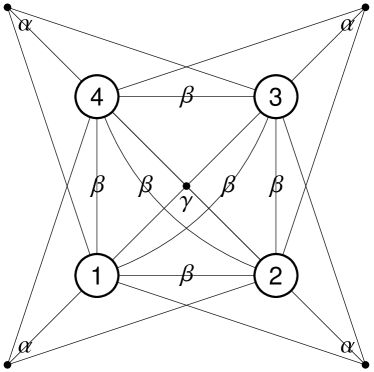
(a)

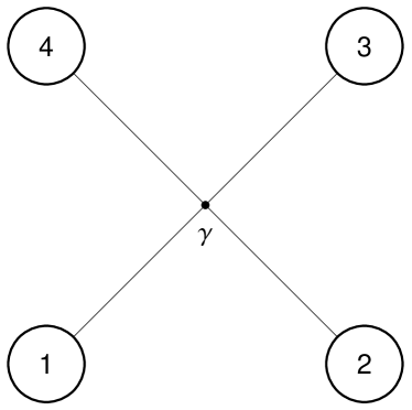
(b)

Figure 2: Graphic representation of the four-vierbein theory in four dimensions. Bi-tetrad interactions are labeled by $\beta$-edges, three-tetrad interactions by $\alpha$-three-vertices and four-tetrad interactions by the $\gamma$-four-vertex. The $\Lambda$-terms (cosmological constants) correspond to self-interacting/closed lines and have not be drawn.

Similarly to the previous section, in order to proceed to the cosmological applications we consider a diagonal FRW ansatz for all the four tetrads (again this means that for the following solutions the Deser-van Nieuwenhuizen condition is satisfied):

$$e_{(1)}{}_{\mu}^{a}=\mbox{diag}\left(N_{a}(t),\frac{a(t)}{\sqrt{1-k\,r^{2}}},a(t)\,r,a(t)\,r\,\sin\theta\right)\,,$$

$$e_{(2)}{}_{\mu}^{a}=\mbox{diag}\left(N_{b}(t),\frac{b(t)}{\sqrt{1-k\,r^{2}}},b(t)\,r,b(t)\,r\,\sin\theta\right)\,,$$

$$e_{(3)}{}_{\mu}^{a}=\mbox{diag}\left(N_{c}(t),\frac{c(t)}{\sqrt{1-k\,r^{2}}},c(t)\,r,c(t)\,r\,\sin\theta\right)\,,$$

$$e_{(4)}{}_{\mu}^{a}=\mbox{diag}\left(N_{d}(t),\frac{d(t)}{\sqrt{1-k\,r^{2}}},d(t)\,r,d(t)\,r\,\sin\theta\right)\,,$$ (5.1)

corresponding to the metrics

$$ds^{2}_{1}=-N_{a}(t)^{2}\,dt^{2}+a(t)^{2}\left(\frac{dr^{2}}{1-kr^{2}}+r^{2}d\Omega^{2}\right)\,,$$

$$ds^{2}_{2}=-N_{b}(t)^{2}\,dt^{2}+b(t)^{2}\left(\frac{dr^{2}}{1-kr^{2}}+r^{2}d\Omega^{2}\right)\,,$$

$$ds^{2}_{3}=-N_{c}(t)^{2}\,dt^{2}+c(t)^{2}\left(\frac{dr^{2}}{1-kr^{2}}+r^{2}d\Omega^{2}\right)\,,$$

$$ds^{2}_{4}=-N_{d}(t)^{2}\,dt^{2}+d(t)^{2}\left(\frac{dr^{2}}{1-kr^{2}}+r^{2}d\Omega^{2}\right)\,.$$ (5.2)

Action variation provides the four first Friedmann equations

$$\frac{\gamma}{M_{1}^{2}}\frac{bcd}{a^{3}}=\frac{k}{a^{2}}+\frac{H_{a}^{2}}{N_{a}^{2}}\,,\quad\frac{\gamma}{M_{2}^{2}}\frac{acd}{b^{3}}=\frac{k}{b^{2}}+\frac{H_{b}^{2}}{N_{b}^{2}}\,,$$

$$\frac{\gamma}{M_{3}^{2}}\frac{abd}{c^{3}}=\frac{k}{c^{2}}+\frac{H_{c}^{2}}{N_{c}^{2}}\,,\quad\frac{\gamma}{M_{4}^{2}}\frac{abc}{d^{3}}=\frac{k}{d^{2}}+\frac{H_{d}^{2}}{N_{d}^{2}}\,,$$ (5.3)

and the four acceleration equations

$$2\dot{H}_{a}+3H_{a}^{2}-2H_{a}\frac{\dot{N}_{a}}{N_{a}}+\frac{k}{a^{2}}N_{a}^{2}=$$

$$\ \ \ \ \ \ \ \ \ \ \frac{\gamma}{M_{1}^{2}}\left(\frac{bc}{a^{2}}N_{a}N_{d}+\frac{bd}{a^{2}}N_{a}N_{c}+\frac{cd}{a^{2}}N_{a}N_{b}\right),$$

$$2\dot{H}_{b}+3H_{b}^{2}-2H_{b}\frac{\dot{N}_{b}}{N_{b}}+\frac{k}{b^{2}}N_{b}^{2}=$$

$$\ \ \ \ \ \ \ \ \ \ \frac{\gamma}{M_{2}^{2}}\left(\frac{ac}{b^{2}}N_{b}N_{d}+\frac{ad}{b^{2}}N_{b}N_{c}+\frac{cd}{b^{2}}N_{a}N_{b}\right),$$

$$2\dot{H}_{c}+3H_{c}^{2}-2H_{c}\frac{\dot{N}_{c}}{N_{c}}+\frac{k}{c^{2}}N_{c}^{2}=$$

$$\ \ \ \ \ \ \ \ \ \ \frac{\gamma}{M_{3}^{2}}\left(\frac{ab}{c^{2}}N_{c}N_{d}+\frac{ad}{c^{2}}N_{b}N_{c}+\frac{bd}{c^{2}}N_{a}N_{c}\right),$$

$$2\dot{H}_{d}+3H_{d}^{2}-2H_{d}\frac{\dot{N}_{d}}{N_{d}}+\frac{k}{d^{2}}N_{d}^{2}=$$

$$\ \ \ \ \ \ \ \ \ \frac{\gamma}{M_{4}^{2}}\left(\frac{ab}{d^{2}}N_{c}N_{d}+\frac{ac}{d^{2}}N_{b}N_{d}+\frac{bc}{d^{2}}N_{a}N_{d}\right),$$ (5.4)

where the parameter $\gamma$ is related to the completely symmetric tensor of coefficients $\chi^{ijkl}$ of equation (2.5) through

$$\gamma=12\,\chi^{1234}\,.$$ (5.5)

In what follows we will consider simple analytical solutions of the four-tetrad theory in vacuum. For simplicity we will not extract matter solutions, having in mind that the analysis of Sec. 4.2 can be generalized here too.

5.1 Vacuum solutions

In this case we can apply the procedure of subsection 4.1 of the three-viebein theory. Doing so we result in one solution (since we have just one interacting term), with $d\propto c\propto b\propto a$ and $N_{b}=b$, $N_{c}=c$, $N_{d}=d$. In order to satisfy the field equations the constants of proportionality must be

$$b=\frac{M_{1}}{M_{2}}\,a\,,\qquad c=\frac{M_{1}}{M_{3}}\,a\,,\qquad d=\frac{M_{1}}{M_{3}}\,a\,.$$ (5.6)

Then setting $N_{a}=1$ the solution for $a$ is

$$a(t)=\frac{kM_{2}M_{3}M_{4}}{a_{0}}\exp\left[-\sqrt{\frac{\gamma M_{1}}{M_{2}M_{3}M_{4}}}t\right]+\frac{a_{0}}{4\gamma M_{1}}\exp\left[\sqrt{\frac{\gamma M_{1}}{M_{2}M_{3}M_{4}}}t\right]\,.$$ (5.7)

This reduces to a de-Sitter expansion if we consider $k=0$, with $\gamma>0$.

All the considerations made in Sec. 4 are generally valid also for this solution. In particular, non-singular bouncing evolution can be realized in vacuum by choosing $a_{0}=\sqrt{4\gamma kM_{1}M_{2}M_{3}M_{4}}$, leading to

$$a(t)=\sqrt{\frac{kM_{2}M_{3}M_{4}}{\gamma M_{1}}}\cosh{\left(\sqrt{\frac{\gamma M_{1}}{M_{2}M_{3}M_{4}}}t\right)}\,,$$ (5.8)

which exhibits a bounce before transiting to an expanding de Sitter universe. Thus, the existence of such behavior seems to be a generic feature of multi-tetrad theories.

6 Discussion and Conclusions

In this work we investigated the cosmology of interacting spin-2 particles. We formulated the full theory in terms of vierbeins, but without imposing the Deser-van Nieuwenhuizen constraint or any similar restriction, which in the general case is not a result of the field equations themselves. Since the imposition of such a restriction assures the equivalence of metric and vielbein formulations of bi-metric theories [39], its absence implies that the resulting multi-vierbein theory is different and much richer than the corresponding multi-metric theory, of which is not even known whether it exists or not. Secondly, since the ghost-freedom for more than two tetrads can be proven only in the vierbein formulation [37], while in the metric description such a general proof does not exist for the moment, even if one finds a way to construct the multi-metric correspondent of the above general multi-vierbein theory, it is not guaranteed that it will be ghost free. The un-restricted multi-vielbein formulation seems to describe a much wider class of theories, which can be used to characterize interacting gravitational sectors. Finally, in order to study the cosmological applications, we introduced the coupling to the matter sector in a self-consistent way.

We studied the cases of three or four interacting vierbeins, focusing on the novel multi-interacting terms that do not have a known multi-metric formulation, setting all the other interacting and non-interacting terms to zero. Clearly, one can study the full interacting theory, or theories with more vierbeins, straightforwardly.

In the case of vacuum solutions we found many de-Sitter expansions, where the effective cosmological constant arises solely from the combination of the multi-interacting terms. Such solutions have a great physical impact since they can describe the inflationary era. In the case where matter is present we found accelerating solutions, which can describe the dark-energy epoch. Additionally, for particular parameter choices we found bouncing behavior.

Finally, we mention that the great complexity that arise in a theory with three or more tetrads does not allow for an analytical treatment of more convoluted cosmological solutions. In order to proceed beyond the extraction of simple and basic analytical solutions one needs to perform numerical elaboration, and indeed in this case he can obtain a richer cosmological behavior, closer to the detailed cosmological history. However, such a detailed numerical investigation lies beyond the aim of the present work, which is to define the cosmology of such theories and to show that at least simple and basic analytical solutions can be constructed.

The above analysis shows that the un-restricted multi-viebein cosmology is richer and includes novel features comparing to bi-metric gravity. Clearly, before accepting such constructions as candidates for the description of nature, many additional investigations should be performed, amongst others the use of observational data in order to constrain the parameters of the theory, a detailed dynamical analysis that could reveal its asymptotic features and the systematic study of the perturbations. These investigations, although necessary, lie beyond the scope of the present work and are left for future investigations.

Appendix A Derivation of the field equations

Consider action (2.1) which we recall for the sake of simplicity

$$S=\int\sum_{i}\mathcal{L}^{(i)}_{\rm EH}+U\,,$$ (A.1)

with

$$U=\epsilon_{abcd}\sum_{i,j,k,l}\tilde{\chi}^{ijkl}\,{\bf e}_{(i)}^{a}\wedge{\bf e}_{(j)}^{b}\wedge{\bf e}_{(k)}^{c}\wedge{\bf e}_{(l)}^{d}\,.$$ (A.2)

In order to extract the field equations for the $i$th tetrad we must vary the action with respect to $e_{(i)}$. The first term in (A.1) will produce the usual Einstein tensor and its variation will not be considered here. The variation of $U$ is

$$\delta_{(i)}U=\epsilon_{abcd}\sum_{j,k,l}\chi^{ijkl}\,\delta{\bf e}_{(i)}^{a}\wedge{\bf e}_{(j)}^{b}\wedge{\bf e}_{(k)}^{c}\wedge{\bf e}_{(l)}^{d}\,,$$ (A.3)

where $\chi^{ijkl}=\mathcal{P}(i)\tilde{\chi}^{ijkl}$, with $\mathcal{P}(i)$ denoting the number of times the $i$th index appears in $\tilde{\chi}^{ijkl}$. This takes into account the number of times $e_{(i)}$ appears inside one term. In other words $\mathcal{P}(i)$ is 1 for ${\bf e}_{(i)}^{a}\wedge{\bf e}_{(j)}^{b}\wedge{\bf e}_{(k)}^{c}\wedge{\bf e}_{(l)}^{d}$, 2 for ${\bf e}_{(i)}^{a}\wedge{\bf e}_{(i)}^{b}\wedge{\bf e}_{(j)}^{c}\wedge{\bf e}_{(k)}^{d}$, 3 for ${\bf e}_{(i)}^{a}\wedge{\bf e}_{(i)}^{b}\wedge{\bf e}_{(i)}^{c}\wedge{\bf e}_{(j)}^{d}$ and 4 for ${\bf e}_{(i)}^{a}\wedge{\bf e}_{(i)}^{b}\wedge{\bf e}_{(i)}^{c}\wedge{\bf e}_{(i)}^{d}$, with $j,k,l$ taking all possible values from 1 to $N$.

At this point Eq. (2.5) follows immediately. To rewrite it as Eq. (2.6) note that

$$\delta_{(i)}U =\epsilon_{abcd}\sum_{j,k,l}\chi^{ijkl}\,\delta{\bf e}_{(i)}^{a}\wedge{\bf e}_{(j)}^{b}\wedge{\bf e}_{(k)}^{c}\wedge{\bf e}_{(l)}^{d}$$

$$=\epsilon_{abcd}\sum_{j,k,l}\chi^{ijkl}\,\delta e_{(i)\mu}^{a}e_{(j)\nu}^{b}e_{(k)\sigma}^{c}e_{(l)\rho}^{d}\epsilon^{\mu\nu\sigma\rho}d^{4}x$$

$$=\delta e_{(i)\mu}^{a}\,e_{(i)e}^{\mu}\,(\det e_{(i)}d^{4}x)\,\epsilon_{abcd}\,\epsilon^{efgh}\sum_{j,k,l}\chi^{ijkl}\,(e_{(i)f}^{\nu}e_{(j)\nu}^{b})(e_{(i)g}^{\sigma}e_{(k)\sigma}^{c})(e_{(i)h}^{\rho}e_{(l)\rho}^{d})$$

$$=\delta e_{(i)\mu}^{a}\,e_{(i)e}^{\mu}\,(\det e_{(i)}d^{4}x)\,\epsilon_{abcd}\,\epsilon^{efgh}\sum_{j,k,l}\chi^{ijkl}\,X_{(ij)}{}_{f}{}^{b}X_{(ik)}{}_{g}{}^{c}X_{(il)}{}_{h}{}^{d}\,.$$ (A.4)

Adding to this the usual variation of the Einstein-Hilbert Lagrangian and then contracting with $e_{(i)\nu}^{a}$, will eventually provide Eq. (2.6).

References

- [1] C. J. Isham, A. Salam and J. A. Strathdee, F-dominance of gravity, Phys. Rev. D 3, 867 (1971).
- [2] D. G. Boulware, S. Deser, Can gravitation have a finite range?, Phys. Rev. D 6, 3368 (1972).
- [3] N. Boulanger, T. Damour, L. Gualtieri and M. Henneaux, Inconsistency of interacting, multigraviton theories, Nucl. Phys. B 597, 127 (2001), [arXiv:hep-th/0007220].
- [4] C. de Rham and G. Gabadadze, Generalization of the Fierz-Pauli Action, Phys. Rev. D 82, 044020 (2010), [arXiv:1007.0443].
- [5] C. de Rham, G. Gabadadze and A. J. Tolley, Resummation of Massive Gravity, Phys. Rev. Lett. 106, 231101 (2011), [arXiv:1011.1232].
- [6] S. F. Hassan, R. A. Rosen and A. Schmidt-May, Ghost-free Massive Gravity with a General Reference Metric, JHEP 1202, 026 (2012), [arXiv:1109.3230].
- [7] S. F. Hassan and R. A. Rosen, Bimetric Gravity from Ghost-free Massive Gravity, JHEP 1202, 126 (2012), [arXiv:1109.3515].
- [8] S. F. Hassan and R. A. Rosen, Confirmation of the Secondary Constraint and Absence of Ghost in Massive Gravity and Bimetric Gravity, JHEP 1204, 123 (2012), [arXiv:1111.2070].
- [9] M. S. Volkov, Cosmological solutions with massive gravitons in the bigravity theory, JHEP 1201, 035 (2012), [arXiv:1110.6153].
- [10] M. von Strauss, A. Schmidt-May, J. Enander, E. Mortsell and S. F. Hassan, Cosmological Solutions in Bimetric Gravity and their Observational Tests, JCAP 1203, 042 (2012), [arXiv:1111.1655].
- [11] M. S. Volkov, Exact self-accelerating cosmologies in the ghost-free bigravity and massive gravity, Phys. Rev. D 86, 061502 (2012)’ [arXiv:1205.5713].
- [12] M. Berg, I. Buchberger, J. Enander, E. Mortsell and S. Sjors, Growth Histories in Bimetric Massive Gravity, JCAP 1212, 021 (2012), [arXiv:1206.3496].
- [13] M. S. Volkov, Exact self-accelerating cosmologies in the ghost-free massive gravity – the detailed derivation, Phys. Rev. D 86, 104022 (2012), [arXiv:1207.3723].
- [14] Y. Akrami, T. S. Koivisto and M. Sandstad, Cosmological constraints on ghost-free bigravity: background dynamics and late-time acceleration, [arXiv:1302.5268].
- [15] S. ’i. Nojiri and S. D. Odintsov, Ghost-free bigravity and accelerating cosmology, Phys. Lett. B 716, 377 (2012), [arXiv:1207.5106].
- [16] S. Capozziello and P. Martin-Moruno, Bounces, turnarounds and singularities in bi-metric gravity, Phys. Lett. B 719, 14 (2013), [arXiv:1211.0214].
- [17] M. Mohseni, Gravitational Waves in Ghost Free Bimetric Gravity, JCAP 1211, 023 (2012), [arXiv:1211.3501].
- [18] S. ’i. Nojiri, S. D. Odintsov and N. Shirai, Variety of cosmic acceleration models from massive bigravity, JCAP 1305, 020 (2013)’ [arXiv:1212.2079].
- [19] K. -i. Maeda and M. S. Volkov, Anisotropic universes in the ghost-free bigravity, [arXiv:1302.6198].
- [20] M. S. Volkov, Self-accelerating cosmologies and hairy black holes in ghost-free bigravity and massive gravity, [arXiv:1304.0238].
- [21] A. De Felice, A. E. Gumrukcuoglu and S. Mukohyama, Massive gravity: nonlinear instability of the homogeneous and isotropic universe, Phys. Rev. Lett. 109, 171101 (2012), [arXiv:1206.2080].
- [22] G. D’Amico, C. de Rham, S. Dubovsky, G. Gabadadze, D. Pirtskhalava and A. J. Tolley, Massive Cosmologies, Phys. Rev. D 84, 124046 (2011), [arXiv:1108.5231].
- [23] A. De Felice, A. E. GÃŒmrÃŒkçÌoÄlu, C. Lin and S. Mukohyama, Nonlinear stability of cosmological solutions in massive gravity, JCAP 1305, 035 (2013), [arXiv:1303.4154].
- [24] A. De Felice, A. E. Gumrukcuoglu, C. Lin and S. Mukohyama, On the cosmology of massive gravity, [arXiv:1304.0484].
- [25] A. E. Gumrukcuoglu, K. Hinterbichler, C. Lin, S. Mukohyama and M. Trodden, Cosmological Perturbations in Extended Massive Gravity, [arXiv:1304.0449].
- [26] F. Kuhnel, On Instability of Certain Bi-Metric and Massive-Gravity Theories, Phys. Rev. D 88, 064024 (2013), [arXiv:1208.1764].
- [27] Y. Akrami, T. S. Koivisto and M. Sandstad, Accelerated expansion from ghost-free bigravity: a statistical analysis with improved generality, JHEP 1303, 099 (2013), [arXiv:1209.0457].
- [28] G. Tasinato, K. Koyama and G. Niz, Vector instabilities and self-acceleration in the decoupling limit of massive gravity, Phys. Rev. D 87, 064029 (2013), [arXiv:1210.3627].
- [29] J. Kluson, Is Bimetric Gravity Really Ghost Free?, [arXiv:1301.3296].
- [30] S. Deser and A. Waldron, Acausality of Massive Gravity, Phys. Rev. Lett. 110, 111101 (2013), [arXiv:1212.5835].
- [31] S. Deser, M. Sandora and A. Waldron, No consistent bi-metric gravity?, [arXiv:1306.0647].
- [32] S. Deser, K. Izumi, Y. C. Ong and A. Waldron, Massive Gravity Acausality Redux, [arXiv:1306.5457].
- [33] S. F. Hassan, A. Schmidt-May and M. von Strauss, Higher Derivative Gravity and Conformal Gravity From Bimetric and Partially Massless Bimetric Theory, [arXiv:1303.6940].
- [34] S. Deser, M. Sandora and A. Waldron, Nonlinear Partially Massless from Massive Gravity?, Phys. Rev. D 87, 101501, (2013), [arXiv:1301.5621].
- [35] C. de Rham, K. Hinterbichler, R. A. Rosen and A. J. Tolley, Evidence for and Obstructions to Non-Linear Partially Massless Gravity, [arXiv:1302.0025].
- [36] J. Kluson, Hamiltonian Formalism of Bimetric Gravity In Vierbein Formulation, [arXiv:1307.1974].
- [37] K. Hinterbichler and R. A. Rosen, Interacting Spin-2 Fields, JHEP 1207 (2012) 047, [arXiv:1203.5783].
- [38] S. Deser and P. van Nieuwenhuizen, Nonrenormalizability of the Quantized Dirac-Einstein System, Phys. Rev. D 10, 411 (1974).
- [39] S. F. Hassan, A. Schmidt-May and M. von Strauss, Metric Formulation of Ghost-Free Multivielbein Theory, [arXiv:1204.5202].
- [40] N. A. Ondo and A. J. Tolley, Complete Decoupling Limit of Ghost-free Massive Gravity, [arXiv:1307.4769].
- [41] C. Deffayet, J. Mourad and G. Zahariade, A note on ’symmetric’ vielbeins in bi-metric, massive, perturbative and non perturbative gravities, JHEP 1303 (2013) 086, [arXiv:1208.4493].
- [42] S. Alexandrov, K. Krasnov and S. Speziale, Chiral description of ghost-free massive gravity, JHEP 1306 (2013) 068, [arXiv:1212.3614].
- [43] H. F. Westman and T. G. Zlosnik, Gravity, Cartan geometry, and idealized waywisers, [arXiv:1203.5709].
- [44] H. F. Westman and T. G. Zlosnik, Cartan gravity, matter fields, and the gauge principle, Annals Phys. 334, 157 (2013), [arXiv:1209.5358].
- [45] T. S. Koivisto, On new variational principles as alternatives to the Palatini method, Phys. Rev. D 83, 101501 (2011), [arXiv:1103.2743].
- [46] J. Beltran Jimenez, A. Golovnev, M. Karciauskas and T. S. Koivisto, The Bimetric variational principle for General Relativity, Phys. Rev. D 86, 084024 (2012), [arXiv:1201.4018].
- [47] N. Tamanini, Variational approach to gravitational theories with two independent connections, Phys. Rev. D 86, 024004 (2012), [arXiv:1205.2511].
- [48] T. S. Koivisto and N. Tamanini, Ghosts in pure and hybrid formalisms of gravity theories: a unified analysis, Phys. Rev. D 87, 104030 (2013), [arXiv:1304.3607].
- [49] N. Khosravi, N. Rahmanpour, H. R. Sepangi and S. Shahidi, Multi-Metric Gravity via Massive Gravity, Phys. Rev. D 85 (2012) 024049, [arXiv:1111.5346].
- [50] K. Nomura and J. Soda, When is Multimetric Gravity Ghost-free?, Phys. Rev. D 86, 084052 (2012), [arXiv:1207.3637].
- [51] Y. .M. Zinoviev, All spin-2 cubic vertices with two derivatives, Nucl. Phys. B 872, 21 (2013); [arXiv:1302.1983].
- [52] P. A. R. Ade et al. [Planck Collaboration], Planck 2013 results. XXIII. Isotropy and Statistics of the CMB, [arXiv:1303.5083].
- [53] S. H. S. Alexander, Is cosmic parity violation responsible for the anomalies in the WMAP data?, Phys. Lett. B 660, 444 (2008), [arXiv:hep-th/0601034].
- [54] T. S. Koivisto and D. F. Mota, CMB statistics in noncommutative inflation, JHEP 1102, 061 (2011), [arXiv:1011.2126].
- [55] Y. Akrami, T. S. Koivisto, D. F. Mota and M. Sandstad, Bimetric gravity doubly coupled to matter: theory and cosmological implications, [arXiv:1306.0004].
- [56] V. Baccetti, P. Martin-Moruno and M. Visser, Null Energy Condition violations in bi-metric gravity, JHEP 1208, 148 (2012), [arXiv:1206.3814].
- [57] S. F. Hassan, A. Schmidt-May and M. von Strauss, JHEP 1305, 086 (2013) [arXiv:1208.1515 [hep-th]].
- [58] N. Tamanini and C. G. Boehmer, Good and bad tetrads in f(T) gravity, Phys. Rev. D 86, 044009 (2012), [arXiv:1204.4593].
- [59] N. Tamanini and C. G. Boehmer, Definition of Good Tetrads for f(T) Gravity, [arXiv:1304.0672].
- [60] T. Biswas, A. Mazumdar and W. Siegel, Bouncing universes in string-inspired gravity, JCAP 0603, 009 (2006), [arXiv:hep-th/0508194].
- [61] T. Biswas, T. Koivisto and A. Mazumdar, Towards a resolution of the cosmological singularity in non-local higher derivative theories of gravity, JCAP 1011, 008 (2010), [arXiv:1005.0590].
- [62] T. Biswas, A. S. Koshelev, A. Mazumdar and S. Y. .Vernov, Stable bounce and inflation in non-local higher derivative cosmology, JCAP 1208, 024 (2012), [arXiv:1206.6374].
- [63] Y. -F. Cai, C. Gao and E. N. Saridakis, Bounce and cyclic cosmology in extended nonlinear massive gravity, JCAP 1210, 048 (2012), [arXiv:1207.3786].
- [64] R. Gannouji, M. . W. Hossain, M. Sami and E. N. Saridakis, Quasi-dilaton non-linear massive gravity: Investigations of background cosmological dynamics, Phys. Rev. D 87, 123536 (2013), [arXiv:1304.5095].
- [65] S. ’i. Nojiri and E. N. Saridakis, Phantom without ghost, Astrophys. Space Sci. 1, 2013 (347), [arXiv:1301.2686].
- [66] T. Qiu, X. Gao and E. N. Saridakis, Towards Anisotropy-Free and Non-Singular Bounce Cosmology with Scale-invariant Perturbations, Phys. Rev. D 88, 043525 (2013), [arXiv:1303.2372].