The Large-Volume Limit of a Quantum Tetrahedron is a Quantum Harmonic Oscillator

Abstract

It is shown that the volume operator of a quantum tetrahedron is, in the sector of large eigenvalues, accurately described by a quantum harmonic oscillator. This result relies on the fact that (i) the volume operator couples only neighboring states of its standard basis, and (ii) its matrix elements show a unique maximum as a function of internal angular momentum quantum numbers. These quantum numbers, considered as a continuous variable, are the coordinate of the oscillator describing its quadratic potential, while the corresponding derivative defines a momentum operator. We also analyze the scaling properties of the oscillator parameters as a function of the size of the tetrahedron, and the role of different angular momentum coupling schemes.

1 Introduction

The quantum volume operator is one of the most studied objects in the field of loop quantum gravity and of crucial importance for the construction of dynamics within this approach [1, 2, 3]. In the literature, one finds traditionally two versions of such an operator, due to Rovelli and Smolin [4], and to Ashtekar and Lewandowski [5], respectively. Their properties and interrelations have been intensively investigated [6, 7, 8, 9, 10, 11, 12, 13, 14, 15, 16, 17, 18, 19, 20, 21, 22, 23], including a third proposal for a volume operator by Bianchi, Dona, and Speziale [20]. The latter one is closer to the concept of spin foams [3] and relies on an older geometric theorem due to Minkowski [24]. Volume operators are usually considered in connection with polyhedra. The most elementary objects of this kind are tetrahedra consisting of four faces which are represented by angular momentum operators coupling to a total spin singlet [11, 25]. Here all three definitions of the volume operator coincide. Among the most recent developments, Bianchi and Haggard have performed a Bohr-Sommerfeld quantization of the volume using an appropriate parameterization of the classical phase space of a tetrahedron, and the obtained semiclassical eigenvalues agree amazingly well with exact numerical data [21, 22].

The purpose of the present communication is to point out that, in the sector of large eigenvalues, the volume operator of such a quantum tetrahedron is accurately described by a quantum harmonic oscillator. Our presentation will continue as follows: After briefly summarizing important features of the quantum tetrahedron and its volume operator in section 2, we derive our central result, starting from numerical observations, in section 3. We give explicit formulae for the large-eigenvalue sector of the (square of the) volume operator and also analyze its scaling behavior as a function of the tetrahedron size. In section 4 we discuss the role of different angular momentum coupling schemes, and in section 5 we close with an outlook.

2 The Quantum Tetrahedron

A quantum tetrahedron consists of four angular momenta $\vec{j}_{i}$, $i\in\{1,2,3,4\}$ representing its faces and coupling to a vanishing total angular momentum [11, 12, 25, 21, 22] , i.e. the Hilbert space consists of all states $|k\rangle$ fulfilling

$$\left(\vec{j}_{1}+\vec{j}_{2}+\vec{j}_{3}+\vec{j}_{4}\right)|k\rangle=0\,.$$ (1)

In what follows we will adopt the coupling scheme where both pairs $\vec{j}_{1},\vec{j}_{2}$ and $\vec{j}_{3},\vec{j}_{4}$ couple first to two irreducible SU(2) representations of dimension $2k+1$ each, which are then added to give a singlet. Thus, the quantum number $k$ ranges as $k_{\rm min}\leq k\leq k_{\rm max}$ with

$$k_{\rm min}=\max\{|j_{1}-j_{2}|,|j_{3}-j_{4}|\}\quad,\quad k_{\rm max}=\min\{j_{1}+j_{2},j_{3}+j_{4}\}\,,$$ (2)

leading to a total dimension of $d=k_{\rm max}-k_{\rm min}+1$. The volume operator can be formulated as

$$V=\frac{\sqrt{2}}{3}\sqrt{|\vec{E}_{1}\cdot(\vec{E}_{2}\times\vec{E}_{3})|}$$ (3)

where the operators

$$\vec{E}_{i}=8\pi\gamma\ell_{P}^{2}\vec{j}_{i}\,,$$ (4)

$i\in\{1,2,3,4\}$ represent the faces of the tetrahedron with $\ell_{P}^{2}=\hbar G/c^{3}$ and $\gamma$ being the Immirzi parameter. As seen form Eq. (3) it is useful to consider the operator

$$\tilde{Q}=\vec{E}_{1}\cdot(\vec{E}_{2}\times\vec{E}_{3})$$ (5)

which, in the basis of the states $|k\rangle$, can be represented as [12, 22, 26, 27, 28]

$$\tilde{Q}=\sum_{k=k_{\rm min}+1}^{k_{\rm max}}i\alpha(k)\left(|k\rangle\langle k-1|-|k-1\rangle\langle k|\right)$$ (6)

with

$$\alpha(k)=2\frac{\Delta(k,j_{1}+1/2,j_{2}+1/2)\Delta(k,j_{3}+1/2,j_{4}+1/2)}{\sqrt{k^{2}-1/4}}\,.$$ (7)

Here $\Delta(a,b,c)$ is the area of a triangle with edges $a,b,c$ expressed via Heron’s formula,

$$\Delta(a,b,c)=\frac{1}{4}\sqrt{(a+b+c)(-a+b+c)(a-b+c)(a+b-c)}\,.$$ (8)

Note that $\tilde{Q}$ couples only basis states $|k\rangle$ with neighboring labels. In the following it will be convenient to readjust the phases of these states via the unitary matrix $u_{\pm}={\rm diag}(1,\pm i,-1,\mp i,1,\dots)$ such that the resulting operator becomes real,

$$u_{\pm}\tilde{Q}u_{\pm}^{+}=:\mp Q=\mp\sum_{k=k_{\rm min}+1}^{k_{\rm max}}\alpha(k)\left(|k\rangle\langle k-1|+|k-1\rangle\langle k|\right)\,.$$ (9)

Since $\tilde{Q}$ is antisymmetric, the spectrum of $\tilde{Q}$ and, in turn, $Q$ consists for even $d$ of pairs of eigenvalues $q,(-q)$ differing in sign. Moreover, because of

$$u\tilde{Q}u^{+}=-\tilde{Q}\quad,\quad uQu^{+}=-Q$$ (10)

with $u=(u_{\pm})^{2}={\rm diag}(1,-1,1,\dots)$, the corresponding eigenstates $|\phi_{q}\rangle$, $|\phi_{-q}\rangle$ fulfill

$$|\phi_{-q}\rangle=u|\phi_{q}\rangle\,.$$ (11)

For odd $d$ an additional zero eigenvalue occurs whose eigenvector (with respect to $\tilde{Q}$) has the unnormalized form [13]

$$|\phi_{0}\rangle \propto \Biggl{(}1,0,\frac{\alpha(k_{\rm min}+1)}{\alpha(k_{\rm min}+2)},0,\frac{\alpha(k_{\rm min}+1)\alpha(k_{\rm min}+3)}{\alpha(k_{\rm min}+2)\alpha(k_{\rm min}+4)},0$$ (12)

$$\quad\dots,\frac{\alpha(k_{\rm min}+1)\alpha(k_{\rm min}+3)\cdots\alpha(k_{\rm max}-1)}{\alpha(k_{\rm min}+2)\alpha(k_{\rm min}+4)\cdots\alpha(k_{\rm max})}\Biggr{)}\,,$$

which is, as it must be, an eigenstate of $u$.

3 Large-Volume Limit

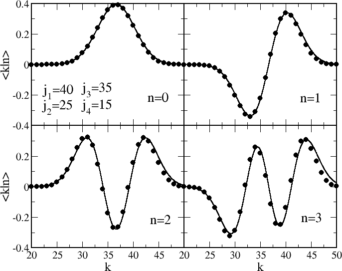
Figure 1: The coefficients $\langle k|n\rangle$ (filled circles) for small $n$ and a typical choice of angular momentum quantum numbers. The solid lines are oscillator wave functions $\psi_{n}(k-\bar{k}+1/2;\omega)$ according to Eq. (20).

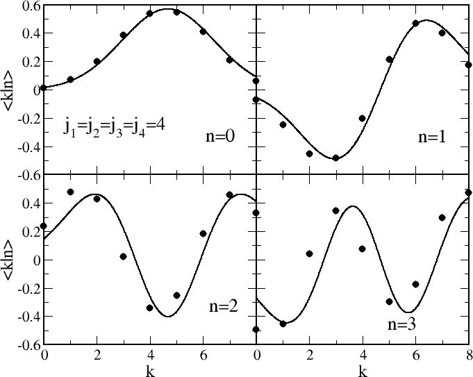
Figure 2: The coefficients $\langle k|n\rangle$ (filled circles) for small $n$ and $j_{i}\equiv 4$. The solid lines are oscillator wave functions $\psi_{n}(k-\bar{k}+1/2;\omega)$ according to Eq. (20).

We denote by $|n\rangle$, $n\in\{0,1,2,\dots\}$, the eigenstates of $Q$ in descending order of eigenvalues with $|0\rangle$ being the state with the largest eigenvalue. In the above basis they can be expanded as

$$|n\rangle=\sum_{k=k_{\rm min}}^{k_{\rm max}}\langle k|n\rangle|k\rangle$$ (13)

where the coefficients $\langle k|n\rangle$ can be viewed as the “wave function” of the state $|n\rangle$ with respect to the “coordinate” $k$. Fig. 1 shows this data for small $n$ and a typical choice of angular momentum quantum numbers (all being of order a few ten). As seen there, the functions $\langle k|n\rangle$ show the characteristic features of wave functions of the harmonic oscillator for low-lying states. Indeed, the solid lines in Fig. 1 are gauss-hermitian oscillator wave functions for parameters to be determined a few lines below. Such properties of the functions $\langle k|n\rangle$ occur for arbitrary sufficiently large angular momentum quantum numbers $j_{i}$ and sets in when all $j_{i}$ exceed a value of about five. For illustration, Fig. 2 displays the data for the case $j_{i}\equiv 4$ where the oscillator-like features of the wave functions gradually disappear with increasing $n$.

The observation made in Figs. 1 and 2 can be explained as follows: Fig. 3 shows the matrix elements $\alpha(k)$ as a function of $k$ for several arbitrary choices of angular momentum lengths including the situation of Fig. 1. In all cases, minima occur at $k\in\{k_{\rm min}+1,k_{\rm max}\}$ with a unique maximum in between at $k=\bar{k}$ determined by

$$\left(\frac{d\alpha(k)}{dk}\right)_{k=\bar{k}}=0\,,$$ (14)

where we have considered $k$ as a continuous variable. The above features can also be established by a detailed analytical discussion of the function $\alpha(k)$.

Now, since the operator $Q$ couples only states with neighboring label $k$, the wave functions with large eigenvalues will have predominantly support around the maximum of $\alpha(k)$. We therefore expand the matrix elements of $Q$ between arbitrary states $|\Phi\rangle$, $|\Psi\rangle$ (lying predominantly in the sector of large eigenvalues) around $\bar{k}$, i.e. $k=\bar{k}-1/2+x$, where the decrement of $(1/2)$ accounts for the fact that $\alpha(\bar{k})$ couples states of the form $|\bar{k}-1\rangle$ and $|\bar{k}\rangle$. In doing so, we obtain

$$\langle\Phi|Q|\Psi\rangle=\sum_{k}\alpha(k)\left(\langle\Phi|k\rangle\langle k-1|\Psi\rangle+\langle\Phi|k-1\rangle\langle k|\Psi\rangle\right)$$

$$\qquad\approx\int dx\,\Phi^{*}(x)\left(2\alpha(\bar{k})+\alpha(\bar{k})\frac{d^{2}}{dx^{2}}+\left(\frac{d^{2}\alpha(k)}{dk^{2}}\right)_{k=\bar{k}}x^{2}\right)\Psi(x)\,.$$ (15)

Here we have introduced the notations $\Phi(x)=\langle\bar{k}+x|\Phi\rangle$, $\Psi(x)=\langle\bar{k}+x|\Psi\rangle$, and additionally performed a continuum approximation to the latter function according to

$$\langle k+1|\Psi\rangle+\langle k-1|\Psi\rangle-2\langle k|\Psi\rangle\approx\frac{d^{2}\Psi(x)}{dx^{2}}\,.$$ (16)

From Eq. (15) one easily reads off an effective operator having the form of a harmonic oscillator,

$$Q_{\rm osc}=\bar{q}\left[1-\left(-\frac{1}{2}\frac{d^{2}}{dx^{2}}+\frac{\omega^{2}}{2}x^{2}\right)\right]$$ (17)

with

$$\bar{q}=2\alpha(\bar{k})$$ (18)

and

$$\omega^{2}=-\frac{\left(\frac{d^{2}\alpha(k)}{dk^{2}}\right)_{k=\bar{k}}}{\alpha(\bar{k})}>0\,.$$ (19)

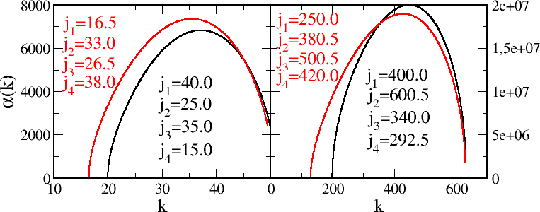
Figure 3: The matrix elements $\alpha(k)$ for various choices of angular momentum quantum numbers. The left panel includes the situation of Fig. 1. In all cases minima occur at $k\in\{k_{\rm min}+1,k_{\rm max}\}$ with a unique maximum in between.

The eigenstates $\psi_{n}(x)=\langle x|n\rangle$ of $Q_{\rm eff}$ are just the well-known wave functions diagonalizing the harmonic oscillator in real-space representation,

$$\psi_{n}(x;\omega)=\sqrt{\frac{1}{n!2^{n}}\sqrt{\frac{\omega}{\pi}}}H_{n}(\sqrt{\omega}x)e^{-\omega x^{2}/2}$$ (20)

where $H_{n}(x)$ are the usual Hermite polynomials. These functions $\psi_{n}(x;\omega)=\psi_{n}(k-\bar{k}+1/2;\omega)$ are plotted as solid lines in Fig. 1 and are remarkably accurate approximations to the coefficients $\langle k|n\rangle$. The corresponding eigenvalues are

$$q_{n}^{\rm osc}=\bar{q}\left(1-\omega(n+1/2)\right)\,.$$ (21)

n	$q_{n}$	$q_{n}^{\rm osc}$	$(q_{n}-q_{n}^{\rm osc})/q_{n}$
0	13141.3	13136.3	$3.8\cdot 10^{-4}$
1	12135.3	12109.8	$2.1\cdot 10^{-3}$
2	11149.4	11083.3	$5.9\cdot 10^{-3}$
3	10183.6	10056.7	$1.2\cdot 10^{-2}$

Table 1: The largest eigenvalues $q_{n}$ of $Q$ obtained by numerical diagonalization of the operator, and the corresponding approximate eigenvalues $q_{n}^{\rm osc}$ according to Eq. (21). The choice of angular momentum quantum numbers is the same as in Fig. 1. The exact and the approximate data agree within a few per mille.

Table 1 compares the largest eigenvalues of $Q$ obtained via exact numerical diagonalization with the approximate results Eq. (21). Both data coincide within a few per mille, in accordance with our previous findings regarding the corresponding eigenvectors. Note that under a rescaling of all four angular momenta, $j_{i}\mapsto uj_{i}$, $\bar{q}$ scales in leading order as $u^{3}$, while for the frequency one finds $\omega\propto 1/u$.

In summary, we have constructed an effective operator describing the sector of large eigenvalues of the square of the volume operator of a quantum tetrahedron. This operator has the form of a harmonic oscillator with a ‘coordinate’$x$ and a ‘momentum’

$$p=-i\frac{d}{dx}$$ (22)

fulfilling the commutation relation

$$[p,x]=-i$$ (23)

which is part of the bedrock of quantum theory.

The approximate data shown in Fig. 1 (solid lines) and table 1 was generated by first finding numerically the maximum position $\bar{k}$ of $\alpha(k)$ and inserting this value into an analytical expression of $(d^{2}\alpha/dk^{2})$ to obtain $\omega$ via Eq. (19). Thus, no adjustable parameter is involved. Closed analytical results for $\bar{k}$ are possible if the four angular momenta come in two pairs of equal length, and the expressions become particularly simple in the case of a regular tetrahedron, $j_{1}=j_{2}=j_{3}=j_{4}=:j$. Here one has

$$\bar{k}^{2} = \frac{2}{3}j(j+1)+\frac{1}{3}+\frac{2}{3}\sqrt{(j(j+1))^{2}-\frac{1}{2}j(j+1)-\frac{1}{8}}$$ (24)

$$= \frac{4}{3}j(j+1)+\frac{1}{6}+{\cal O}\left(\frac{1}{j}\right)$$ (25)

such that the parameters entering the effective operator (17) are given, to leading orders in $j$, by

$$\bar{q}=\frac{4}{3\sqrt{3}}\left(j(j+1)\right)^{3/2}+{\cal O}\left(j\right)\,,$$ (26)

$$\left(\frac{d^{2}\alpha(k)}{dk^{2}}\right)_{k=\bar{k}}=-\sqrt{\frac{3}{2}j(j+1)}+{\cal O}\left(\frac{1}{j}\right)\,,$$ (27)

$$\omega^{2}=\frac{9/4}{j(j+1)}+{\cal O}\left(\frac{1}{j^{3}}\right)\,.$$ (28)

Thus, the eigenvalues (21) of the effective operator read to the first leading orders in $j$

$$q_{n}^{\rm osc}=\frac{4}{3\sqrt{3}}\left(j^{3}+\frac{3}{2}j^{2}\right)-\frac{2}{\sqrt{3}}j^{2}\left(n+\frac{1}{2}\right)+{\cal O}\left(j\right)\,.$$ (29)

In particular, from Eq. (28) we see that the width $1/\sqrt{\omega}$ of the wave functions (20) is proportional to $\sqrt{j(j+1)}$. Moreover, for the largest eigenvalue of the volume operator, one finds from Eq. (3)

$$\frac{V_{0}}{(8\pi\gamma\ell_{P})^{3/2}}\approx\frac{\sqrt{2}}{3}\sqrt{q^{\rm osc}_{0}}=\frac{2^{3/2}}{3^{7/4}}j^{3/2}\left(1-\frac{3}{8}\frac{1}{j}\right)+{\cal O}\left(\frac{1}{\sqrt{j}}\right)\,.$$ (30)

Here the leading term $(\propto j^{3/2})$ is exactly the classical volume of a regular tetrahedron whose faces have area $j$, and the subleading correction is, after a redefinition of the face area, identical to the one found in Ref. [22] using Bohr-Sommerfeld quantization. Furthermore, our findings here suggest that the classical volume of a general tetrahedron with face areas $j_{1},j_{2},j_{3},j_{4}$ is, to leading order in all $j_{i}$, given by

$$V_{\rm cl}=\frac{2}{3}\sqrt{\alpha(\bar{k})}\,.$$ (31)

As already discussed in section 2, the large eigenvalues $q_{n}$ have counterparts $q_{n}^{\prime}=-q_{n}$ with the the same modulus but negative sign, and according to Eq. (11), the pertaining eigenvectors can be obtained from the previous ones by changing the sign of any other component. Regarding the wave functions (20) one could try to mimic this behavior by attaching an appropriate phase factor,

$$\psi_{n}^{\prime}(x)=e^{i\pi x}\psi_{n}(x)\,.$$ (32)

However, the above functions are clearly not eigenfunctions of the effective operator (17). In fact, an operator having $\psi_{n}^{\prime}$ as eigenstates with eigenvalues $(-q_{n}^{\rm osc})$ can be constructed as follows:

$$Q_{\rm osc}^{\prime} = -e^{i\pi x}Q_{\rm osc}e^{-i\pi x}$$ (33)

$$= -\bar{q}\left[1-\left(\frac{1}{2}\left(p-\pi\right)^{2}+\frac{\omega^{2}}{2}x^{2}\right)\right]\,.$$ (34)

This operator is not invariant under a ‘time reversal’$p\mapsto-p$ which corresponds to the fact that the eigenfunctions (32) cannot be chosen to be real. Moreover, the operators $Q_{\rm osc}$ and $Q_{\rm osc}^{\prime}$ are, along with their eigenfunctions, obviously just related by a U(1) gauge operation, apart from the global minus sign on the r.h.s of Eqs. (33) and (34). However, since $Q_{\rm osc}^{\prime}$ is merely a consequence of the rather phenomenological ansatz (32), a more rigorous effective description of eigenstates with negative eigenvalue is desirable. Work in this direction could possibly build upon ideas of Ref. [23] where the quantity $\pm 2\alpha(k)$ was considered as an effective potential for states with eigenvalues of both sign.

4 Recoupling of Angular Momenta

There are obviously alternatives to the coupling scheme of angular momenta we have used so far. For instance, instead of the previous procedure, $\vec{j}_{1},\vec{j}_{3}$ and $\vec{j}_{2},\vec{j}_{4}$ could first be coupled to two irreducible representations of dimension $2l+1$ each, which are then combined to a total singlet. The operator $Q$ is then expressed in a form analogous to Eq. (9) with matrix elements $\beta(l)$ given by the r.h.s of Eq. (7) and obvious interchanges of labels. As seen before, $\beta(l)$ has a unique maximum at some $l=\bar{l}$. Thus, putting again $l=\bar{l}+y-1/2$, the eigenstates with large eigenvalues will again be accurately approximated by oscillator wave functions $\psi_{n}(y;\nu)$ according to Eq. (20) with

$$\nu^{2}=-\frac{\left(\frac{d^{2}\beta(l)}{dl^{2}}\right)_{l=\bar{l}}}{\beta(\bar{l})}\,,$$ (35)

and the corresponding approximate eigenvalues read

$$q_{n}^{\rm osc}=\bar{r}\left(1-\nu(n+1/2)\right)$$ (36)

with $\bar{r}=2\beta(\bar{l})$.

Since the exact spectrum of $Q$ is of course independent of the coupling scheme used, this holds as well, to an excellent degree of approximation, for the approximate eigenvalues, as it is easily checked by numerics. For instance, for the parameters of Fig. 1 and table  1 we find $\bar{q}=13649.6$, $\bar{r}=13650.4$ and $\omega=0.075206$, $\nu=0.075198$. Thus, we have, as an again excellent approximation,

$$\omega\approx\nu\,,$$ (37)

which in particular means that the wave functions $\psi_{n}(x;\omega)$ and $\psi_{n}(y;\nu)$ can be taken as identical.

Moreover, since switching to another coupling scheme implies just a change of basis in the Hilbert space, the above two gauss-hermitian wave functions should be related by a unitary transformation,

$$\eta_{n}\psi_{n}(y;\omega)=\int dx\,U(y,x)\psi_{n}(x;\omega)\,,$$ (38)

with some phase factor $\eta_{n}$, $|\eta_{n}|=1$. An obvious solution is given by $\eta_{n}\equiv 1$ and $U(y,x)=\delta(y-x)$, while another possibility follows from the well-known fact that the Fourier transform of a gauss-hermitian function is a function of that same type: Here one has $\eta_{n}=(-i)^{n}$ and

$$U(y,x)=\sqrt{\frac{\omega}{2\pi}}e^{-i\omega yx}\,.$$ (39)

Thus, up to the scale factor $\omega$ occurring in Eq. (39), changing from one coupling scheme to another just corresponds to a Fourier transform of the approximating oscillator wave functions. This observation is of course strongly reminiscent of switching from real space to momentum representation in standard quantum mechanics.

On the other hand, treating $k$ and $l$ again as discrete state labels, the basis states in both coupling schemes are related by

$$|l\rangle=\sum_{k=k_{\rm min}}^{k_{\rm max}}(-1)^{j_{2}+j_{3}+k+l}\sqrt{(2k+1)(2l+1)}\left\{\begin{array}[]{ccc}j_{1}&j_{2}&k\\ j_{4}&j_{3}&l\end{array}\right\}|k\rangle\,,$$ (40)

using Wigner $6j$-symbols in the standard convention of prefactors [28]. For the case of all angular momenta being large compared to unity, Ponzano and Regge [29] have devised the following asymptotic expression for such quantities (for more recent developments, see also Refs. [30, 31, 32]),

$$\left\{\begin{array}[]{ccc}j_{1}&j_{2}&j_{3}\\ j_{4}&j_{5}&j_{6}\end{array}\right\}\approx\frac{1}{\sqrt{12\pi{\cal V}}}\cos\left(\frac{\pi}{4}+\sum_{i=1}^{6}\theta_{i}(j_{i}+1/2)\right)\,.$$ (41)

Here $\cal V$ is the volume of a tetrahedron having edge lengths $(j_{i}+1/2)$, $i\in\{1\dots 6\}$ where edges occurring in the same column of the $6j$-symbol are opposite to each other, i.e. do not have a common vertex, and $\theta_{i}$ is the external dihedral angle between faces joining at edge $j_{i}$. The cosine occurring in the above equation bears some similarity to the exponential in the transformation (39). Moreover, under a rescaling of all angular momenta, $j_{i}\mapsto uj_{i},k\mapsto uk,l\mapsto ul$, $\cal V$ scales obviously as $u^{3}$, such that the prefactor of $|uk\rangle$ in Eq. (40) is proportional to $1/\sqrt{u}$, which is the same scaling behavior as in (39). However, we leave it to future studies to more deeply investigate the possible relationship between the transformations (39) and (40).

5 Conclusions and Outlook

We have shown that the (square of the) volume operator of a quantum tetrahedron is, in the sector of large egenvalues, accurately desribed by a quantum harmonic oscillator. This finding is a consequence of the fact that (i) the volume operator couples only neighboring states of its standard basis, and (ii) its matrix elements show a unique maximum as a function of state labels. The ingredients of the harmonic oscillator constructed here are an appropriate coordinate variable and a momentum operator defined by the corresponding derivative. These two quantities fulfill the canonical commutation relation.

We give explicit formulae for the large eigenvalues of the volume operator in terms of the equidistant harmonic oscillator spectrum. It is an interesting speculation whether or not these linear excitations of space are related to gravitational waves. Moreover, in this limit the quantum tetrahedron is naturally described semiclassically by oscillator coherent states, in contrast to other approaches where tensor products of SU(2) coherent states projected onto the singlet subspace are used [33, 3].

We have also analyzed the scaling properties of the oscillator parameters as a function of the size of the tetrahedron. For a regular tetrahedron we reproduce recent findings [22] on the largest volume eigenvalue and generalize them to the next smaller eigenvalues. In terms of classical geometry, our approach here also suggests an interesting expression given in Eq. (31) for the volume of a general tetrahedron. To further investigate this conjecture might be, from a more mathemaitcal perspective, a route for future studies (possibly starting from numerical tests). Here we have shown the result only for the very special case of a regular tetrahedron. Finally, we have discussed the role of different angular momentum coupling schemes.

One might argue that the findings here on the tetrahedral volume operator are in fact very general: Expanding a classical system described by just one pair of canonical variables [21, 22] around an extremum will generically lead to an effective harmonic oscillator. An interesting point here is that this oscillator-like behavior sets in at already quite moderate lengths of the involved angular momenta (being about five). Moreover, the quantum number resulting from the coupling of angular momenta has an immediate interpretation in terms of the oscillator coordinate.

The present work exclusively deals with tetrahedra, i.e., in the language of spin networks, 4-valent nodes [3]. An obvious and interesting question is how the results found here translate to higher nodes. Recent work, in a similar spirit as here, on the semiclassical properties of pentahedra includes Refs. [34, 35].

References

References

- [1] C. Rovelli, Quantum Gravity, Cambridge University Press 2004.
- [2] T. Thiemann, Modern Canonical Quantum General Relativity, Cambridge University Press 2007.
- [3] A. Perez, Living. Rev. Relativity 16, 3 (2013), arXiv:1205.2019.
- [4] C. Rovelli and L. Smolin, Nucl. Phys. B 442, 593 (1995), arXiv:gr-qc/9411005.
- [5] A. Ashtekar and J. Lewandowski, J. Geom. Phys. 17, 191 (1995), arXiv:gr-qc/9412073.
- [6] R. Loll, Phys. Rev. Lett. 75, 3048 (1995), arXiv:gr-qc/9506014.
- [7] R. Loll, Nucl. Phys. B 460, 143 (1996), arXiv:gr-qc/9511030
- [8] R. De Pietri and C. Rovelli, Phys. Rev. D 54, 2664 (1996), arXiv:gr-qc/9602023.
- [9] R. De Pietri, Nucl. Phys. Proc. Suppl. 57, 251 (1997), arXiv:gr-qc/9701041.
- [10] T. Thiemann, J. Math. Phys. 39, 3347 (1998), arXiv:gr-qc/9606091.
- [11] A. Barbieri, Nucl. Phys. B 518, 714 (1998), arXiv:gr-qc/9707010.
- [12] G. Carbone, M. Carfora, and A. Marzuoli, Class. Quant. Grav. 19, 3761 (2002), arXiv:gr-qc/0112043.
- [13] J. Brunnemann and T. Thiemann, Class. Quant. Grav. 23, 1289 (2006), arXiv:gr-qc/0405060.
- [14] K. Giesel and T. Thiemann, Class. Quant. Grav. 23, 5693 (2006), arXiv:gr-qc/0507037.
- [15] K. Giesel and T. Thiemann, Class. Quant. Grav. 23, 5667 (2006), arXiv:gr-qc/0507036.
- [16] K. A. Meissner, Class. Quant. Grav. 23, 617 (2006), arXiv:gr-qc/0509049.
- [17] J. Brunnemann and D. Rideout, Class. Quant. Grav. 25, 065001 (2008), arXiv:0706.0469 [gr-qc].
- [18] J. Brunnemann and D. Rideout, Class. Quant. Grav. 25, 065002 (2008), arXiv:0706.0382 [gr-qc].
- [19] B. Dittrich and T. Thiemann, J. Math. Phys. 50, 012503 (2009), arXiv:0708.1721 [gr-qc].
- [20] E. Bianchi, P. Dona, and S. Speziale, Phys. Rev. D 83, 044035 (2011), arXiv:1009.3402 [gr-qc].
- [21] E. Bianchi and H. M. Haggard, Phys. Rev. Lett. 107, 011301 (2011), arXiv:1102.5439 [gr-qc].
- [22] E. Bianchi and H. M. Haggard, Phys. Rev. D 86, 124010 (2013), arXiv:1208.2228.
- [23] V. Aquilanti, D. Marinelli, and A. Marzuoli, J. Phys. A: Math. Theor. 46, 175303 (2013), arXiv:1301.1949 [quant-ph].
- [24] H. Minkowski, Nachr. Kgl. Ges. d. W. Gött., Math-Phys. Klasse 1897, 198.
- [25] J. C. Baez and J. W. Barrett, Adv. Theor. Math. Phys. 3, 815 (1999), arXiv:gr-qc/9903060.
- [26] J.-M. Levy-Leblond and M. Levy-Nahas, J. Math. Phys. 6, 1372 (1965).
- [27] A. Chakrabarti, Ann. H. Poincare A 1, 301 (1964).
- [28] A. R. Edmonds, Angular Momentum in Quantum Mechanics, Princeton University Press 1957.
- [29] G. Ponzano and T. Regge, in Spectroscopic and group theoretical methods, edited by F. Bloch et al., North-Holland, Amsterdam 1968.
- [30] R. Gurau, Ann. H. Poincare 9, 1413 (2008), arXiv:0808.3533 [math-ph].
- [31] M. Dupuis and E. R. Livine, Phys. Rev D 80, 024035 (2009), arXiv:0905.4188 [gr-qc].
- [32] V. Aquilanti, H. M. Haggard, A. Hedeman, N. Jeevanjee, R. G. Littlejohn, and L. Yu, J. Phys A: Math. Theor. 45, 065209 (2012), arXiv:1009.2811 [math-ph].
- [33] E. R. Livine and S. Speziale, Phys. Rev D 76, 084028 (2007), arXiv:0705.0674 [gr-qc].
- [34] H. M. Haggard, Phys. Rev D 87, 044020 (2013), arXiv:1211.7311 [gr-qc].
- [35] C. E. Coleman-Smith and B. Müller, Phys. Rev D 87, 044047 (2013), arXiv:1212.1930 [gr-qc].