On data-based optimal stopping under stationarity and ergodicity

Abstract

The problem of optimal stopping with finite horizon in discrete time is considered in view of maximizing the expected gain. The algorithm proposed in this paper is completely nonparametric in the sense that it uses observed data from the past of the process up to time $-n+1$, $n\in\mathbb{N}$, not relying on any specific model assumption. Kernel regression estimation of conditional expectations and prediction theory of individual sequences are used as tools. It is shown that the algorithm is universally consistent: the achieved expected gain converges to the optimal value for $n\to\infty$ whenever the underlying process is stationary and ergodic. An application to exercising American options is given, and the algorithm is illustrated by simulated data.

and

1 Introduction

In this paper an optimal stopping problem with finite horizon $L$ in discrete time is treated. The problem is formulated as follows: Let $(Z_{j})_{j\in\mathbb{Z}}$ be a sequence of real-valued random variables and let $g_{j}(Z_{1}^{j})$, with measurable bounded and real-valued functions $g_{j}$ on $\mathbb{R}^{j}$ $(g_{0}=\mathit{const})$ and notation $Z_{1}^{j}=(Z_{1},\dots,Z_{j})$, be the gain when stopping at time $j$ $(j\in\{0,1,\dots,L\})$. In case that one stops at time $k\in\{0,1,\dots,L\}$ any stopping rule can rely only on the observed values of $Z_{j}$ at times $j\leq k$. Therefore, it can be described by a stopping time $\tau$, that is, by a measurable function of $Z_{-\infty}^{L}:=(\dots,Z_{-1},Z_{0},\dots,Z_{L})$ where the event $[\tau=k]$ is contained in the $\sigma$-algebra $\mathcal{F}(Z_{-\infty}^{k})$ generated by $Z_{-\infty}^{k}$. Let $\mathcal{T}(0,1,\dots,L)$ be the set of all such stopping times. Any stopping time $\tau\in\mathcal{T}(0,1,\dots,L)$ yields the expected gain

$$\mathbf{E}\bigl{\{}g_{\tau}\bigl{(}Z_{1}^{\tau}\bigr{)}\bigr{\}},$$

and it is this quantity which one wants to maximize, that is, one wants to construct a stopping time $\tau^{*}\in\mathcal{T}(0,1,\dots,L)$ such that

$$V_{0}^{*}:=\sup_{\tau\in\mathcal{T}(0,\dots,L)}\mathbf{E}\bigl{\{}g_{\tau}\bigl{(}Z_{1}^{\tau}\bigr{)}\bigr{\}}=\mathbf{E}\bigl{\{}g_{\tau^{*}}\bigl{(}Z_{1}^{\tau^{*}}\bigr{)}\bigr{\}}$$

(so-called value of the optimal stopping problem). In the sequel, we assume only stationarity and ergodicity and define decision rules on the basis of observed data. The unknown underlying distribution is not used.

More precisely, for $n\in\mathbb{N}$ we assume that from the past of the process the random variables $Z_{-n+1},\dots,Z_{0}$ are observed and we want to construct a stopping time

$$\hat{\tau}_{n}=\hat{\tau}_{n}\bigl{(}Z_{-n+1}^{L}\bigr{)}\in\mathcal{T}(0,1,\dots,L)$$

such that

$$\hat{V}_{0,n}:=\mathbf{E}\bigl{\{}g_{\hat{\tau}_{n}}\bigl{(}Z_{1}^{\hat{\tau}_{n}}\bigr{)}\bigr{\}}$$

converges to $V_{0}^{*}$.

In the definition of our estimates, we firstly use results from the general theory of optimal stopping showing that an optimal stopping time can be constructed on the basis of dynamic programming by recursively computing so-called continuation value functions, which indicate the value of the optimal stopping problem (from time $t$ on) given an observed vector $Z_{-\infty}^{t}$ under the constraint of no stopping at time $t$ (cf., e.g., Chow, Robbins and Siegmund [3] or Shiryayev [16]). Secondly, we use that these continuation values can be represented as conditional expectations (cf., e.g., Tsitsiklis and van Roy [17], Longstaff and Schwarz [14] or Egloff [5]), and our algorithm uses techniques from nonparametric regression to estimate these conditional expectations from observed stationary and ergodic data $Z_{-n+1}$, $Z_{-n}$, …. In contrast to the above references which study regression-based Monte-Carlo methods for pricing American options, for our estimates we do not use simulations of the underlying process, because in our case its distribution is unknown, but use only the observation of the individual sequence back to time $-n+1$. This is in general a rather challenging task, where usually extremely complex and data consuming algorithms are necessary (cf., e.g., Morvai, Yakowitz and Györfi [15]). But in case that it is enough to construct algorithms which converge in the so-called Cesàro sense, a relatively simple and nice algorithm exists (cf., e.g., Section 27.5 in Györfi et al. [7]), which uses techniques from the theory of prediction of individual sequences (cf., e.g., Cesa-Bianchi and Lugosi [2]). These techniques have already been used successfully in the context of portfolio optimization (cf., e.g., Györfi, Lugosi and Udina [8], Györfi, Udina and Walk [9] and the references therein). In this paper, we introduce as main trick an averaging of such estimates and show that by using this trick we can derive a consistency result of our estimated stopping rule from Cesàro consistency of the underlying regression estimates. So in the definition of our estimate, we thirdly apply estimates defined by use of ideas from the prediction theory of individual sequences.

As an application, we consider the problem of exercising an American option in discrete time (also called Bermudan option) in view of maximizing of the expected discounted payoff.

The algorithm computing estimates of the optimal stopping time is described in Section 2 and the main result is formulated in Section 3, where also an application to American options is described. In Section 4, we illustrate our algorithm by applying it to simulated data, Section 5 contains the proof of the main result, the proof of an auxiliary result is given in the Appendix.

2 Construction of an approximation of the optimal stopping time

Our first idea is to use results from the general theory of optimal stopping in order to determine the optimal stopping time $\tau^{*}$. Let $t\in\{0,\dots,L-1\}$ be fixed and denote the set of all stopping times with values in $\{t+1,\dots,L\}$ by $\mathcal{T}(t+1,\dots,L)$.

For each $\tau\in\mathcal{T}(t+1,\dots,L)$, define the real random variable $h_{\tau}$ on the probability space $(\prod_{-\infty}^{t}\mathbb{R},\bigotimes_{-\infty}^{t}\mathcal{B},\mathbf{P}_{Z_{-\infty}^{t}})$ with Borel product $\sigma$-algebra and distribution of $Z_{-\infty}^{t}$ by

$$h_{\tau}\bigl{(}z_{-\infty}^{t}\bigr{)}:=\mathbf{E}\bigl{\{}g_{\tau}\bigl{(}Z_{1}^{\tau}\bigr{)}|Z_{-\infty}^{t}=z_{-\infty}^{t}\bigr{\}}.$$

Then, according to Chow, Robbins and Siegmund [3], Section 7.6,

$$\operatorname{ess}\sup_{\tau\in\mathcal{T}(t+1,\dots,L)}h_{\tau}=:q_{t}$$

is defined as a real-valued random variable $y$ on this probability space such that

1. [(ii)]

2. $\mathbf{P}_{Z_{-\infty}^{t}}\{y\geq h_{\tau}\}=1$ for every $\tau\in\mathcal{T}(t+1,\dots,L)$,

3. if $y^{\prime}$ is any real random variable on the probability space satisfying

   $$\mathbf{P}_{Z_{-\infty}^{t}}\bigl{\{}y^{\prime}\geq h_{\tau}\bigr{\}}=1\qquad\mbox{for every }\tau\in\mathcal{T}(t+1,\dots,L),$$

   then

   $$\mathbf{P}_{Z_{-\infty}^{t}}\bigl{\{}y^{\prime}\geq y\bigr{\}}=1.$$

Thus, $q_{t}$ is unique $mod$ $\mathbf{P}_{Z_{-\infty}^{t}}$, that is, two versions of $q_{t}$ coincide $\mathbf{P}_{Z_{-\infty}^{t}}$-almost everywhere. By Theorem 1.5 in Chow, Robbins and Siegmund [3], $q_{t}$ always exists, and there exists a countable subset $\mathcal{T}_{t}^{*}$ of $\mathcal{T}(t+1,\dots,L)$ such that

$$q_{t}=\sup_{\tau\in\mathcal{T}_{t}^{*}}h_{\tau}.$$

Furthermore we set $q_{L}:=0$. $q_{t}$ is denoted as continuation value function $(t\in\{0,\dots,L\})$.

The so-called continuation values

$$q_{t}\bigl{(}z_{-\infty}^{t}\bigr{)} \hskip 2.8pt=: \operatorname{ess}\sup_{\tau\in\mathcal{T}(t+1,\dots,L)}\mathbf{E}\bigl{\{}g_{\tau}\bigl{(}Z_{1}^{\tau}\bigr{)}|Z_{-\infty}^{t}=z_{-\infty}^{t}\bigr{\}}\qquad\bigl{(}t\in\{0,\dots,L-1\}\bigr{)},$$

$$q_{L}\bigl{(}z_{-\infty}^{L}\bigr{)} = 0$$

describe the values of the optimal stopping problem from $t$ on given $Z_{-\infty}^{t}=z_{-\infty}^{t}$ subject to the constraint of not stopping at time $t$.

Replacing $\mathcal{T}(t+1,\dots,L)$ by $\mathcal{T}(t,\dots,L)$ leads to the so-called value functions

$$\operatorname{ess}\sup_{\tau\in\mathcal{T}(t,\dots,L)}h_{\tau}=:V_{t}\qquad\bigl{(}t\in\{0,\dots,L\}\bigr{)}.$$ (1)

$V_{t}(z_{-\infty}^{t})$ describes the value of the optimal stopping problem (from $t$ on) given $Z_{-\infty}^{t}=z_{-\infty}^{t}$.

For $t\in\{-1,0,\dots,L-1\}$, set

$$\tau_{t}^{*}:=\inf\bigl{\{}s\geq t+1\colon\ q_{s}\bigl{(}Z_{-\infty}^{s}\bigr{)}\leq g_{s}\bigl{(}Z_{1}^{s}\bigr{)}\bigr{\}}.$$ (2)

We can conclude from the general theory of optimal stopping (see, e.g., Chow, Robbins and Siegmund [3] or Shiryayev [16]).

Lemma 2.1

It holds

$$V_{t}\bigl{(}z_{-\infty}^{t}\bigr{)}=\mathbf{E}\bigl{\{}g_{\tau_{t-1}^{*}}\bigl{(}Z_{1}^{\tau_{t-1}^{*}}\bigr{)}|Z_{-\infty}^{t}=z_{-\infty}^{t}\bigr{\}}$$ (3)

$\mathbf{P}_{Z_{-\infty}^{t}}$-almost everywhere for $t\in\{0,\dots,L\}$. Furthermore

$$V_{0}^{*}:=\sup_{\tau\in\mathcal{T}(0,\dots,L)}\mathbf{E}\bigl{\{}g_{\tau}\bigl{(}Z_{1}^{\tau}\bigr{)}\bigr{\}}=\mathbf{E}\bigl{\{}g_{\tau^{*}}\bigl{(}Z_{1}^{\tau^{*}}\bigr{)}\bigr{\}}$$ (4)

is fulfilled for

$$\tau^{*}:=\tau^{*}_{-1}=\inf\bigl{\{}j\in\{0,1,\dots,L\}\colon\ g_{j}\bigl{(}Z_{1}^{j}\bigr{)}\geq q_{j}\bigl{(}Z_{-\infty}^{j}\bigr{)}\bigr{\}}.$$

Lemma 2.1 can be proven as in the case of Markovian processes (cf., e.g., proof of Theorem 1 in Kohler [11]), a complete proof of this lemma is available from the authors by request.

From Lemma 2.1, we get that it suffices to compute the continuation value functions $q_{0}$, …, $q_{{L-1}}$ in order to construct the optimal stopping rule $\tau^{*}$. In Tsitsiklis and van Roy [17], Longstaff and Schwarz [14] and Egloff [5] it is shown that in case of Markovian processes the continuation values can be computed recursively by evaluation of conditional expectations. The same can be shown also in the setting considered in this paper.

Lemma 2.2

The continuation values satisfy

$$q_{j}\bigl{(}z_{-\infty}^{j}\bigr{)}=\mathbf{E}\bigl{\{}\max\bigl{\{}g_{j+1}\bigl{(}Z_{1}^{j+1}\bigr{)},q_{j+1}\bigl{(}Z_{-\infty}^{j+1}\bigr{)}\bigr{\}}|Z_{-\infty}^{j}=z_{-\infty}^{j}\bigr{\}}$$ (5)

$\mathbf{P}_{Z_{-\infty}^{j}}$-almost everywhere and

$$q_{j}\bigl{(}z_{-\infty}^{j}\bigr{)}=\mathbf{E}\bigl{\{}g_{\tau_{j}^{*}}\bigl{(}Z_{1}^{\tau_{j}^{*}}\bigr{)}|Z_{-\infty}^{j}=z_{-\infty}^{j}\bigr{\}}$$ (6)

$\mathbf{P}_{Z_{-\infty}^{j}}$-almost everywhere for any $j\in\{0,1,\dots,L-1\}$.

Lemma 2.2 can be proven as in the case of Markovian processes (cf., e.g., proof of Theorem 2 in Kohler [11]), again a complete proof of this lemma is available from the authors by request.

Usually in applications, the distribution of the underlying process $(Z_{n})_{n}$ is unknown and therefore it is impossible to use (5) (or (6)) in order to compute the continuation values. In the sequel, we will try to estimate them by using (recursively defined) regression estimates in order to approximate the conditional expectations in (5). To do this, for any $n\in\mathbb{N}$ we use $Z_{-n+1}^{0}$ in order to construct an estimate of the optimal stopping rule on the data $Z_{0}$, …, $Z_{L}$.

Next, we describe how we construct estimates $\hat{q}_{j}^{(n)}(Z_{-n+1}^{j})$ of $q_{j}(Z_{-\infty}^{j})$.

The estimates are defined recursively with respect to $j\in\{0,\dots,L\}$. For $j=L$, we have $q_{L}=0$ and in this case we set

$$\hat{q}_{L}^{(n)}:=0.$$

Given $\hat{q}_{j+1}^{(m)}$ (defined on $\mathbb{R}^{j+m+1}$), $m\leq n$, for some $j\in\{0,1,\dots,L-1\}$ we define $\hat{q}_{j}^{(n)}$ as follows.

To make the construction more transparent, for the function $q_{j}\mathchoice{\nobreak\,\colon}{\nobreak\,\colon}{\nobreak\,\colon\;}{\nobreak\,\colon\;}\prod_{-\infty}^{j}\mathbb{R}\rightarrow\mathbb{R}$, which by (5) is given as a regression function, we define a regression estimation function $\hat{m}^{(n)}_{j,(k,h)}(z_{-n+1}^{0};\cdot)\mathchoice{\nobreak\,\colon}{\nobreak\,\colon}{\nobreak\,\colon\;}{\nobreak\,\colon\;}\prod_{-n+1}^{j}\mathbb{R}\rightarrow\mathbb{R}_{+}$ with parameters $k$, $h$ using realizations $z_{-n+1}^{0}$ of $Z_{-n+1}^{0}$. The definition depends on parameters $k\in\mathbb{N}$ (indicating how far back the estimate will look, and thus indicating also the dimension of the occurring regression estimation problem) and $h>0$ (a so-called bandwidth which (roughly speaking) indicates how similar observed values in the past must be to the current observed values in order to be included in the prediction of the future value) and a kernel function $K\mathchoice{\nobreak\,\colon}{\nobreak\,\colon}{\nobreak\,\colon\;}{\nobreak\,\colon\;}\mathbb{R}^{j+k+1}\rightarrow\mathbb{R}_{+}$. We define the latter by

$$K(v):=H\bigl{(}\|v\|_{2}^{j+k+1}\bigr{)},$$

where $\|v\|_{2}$ denotes the Euclidean norm of $v$ and $H\mathchoice{\nobreak\,\colon}{\nobreak\,\colon}{\nobreak\,\colon\;}{\nobreak\,\colon\;}\mathbb{R}_{+}\rightarrow\mathbb{R}_{+}$ is a given nonincreasing and continuous function satisfying

$$H(0)>0\quad\mbox{and}\quad t\cdot H(t)\rightarrow 0\qquad(t\rightarrow\infty)$$

(e.g., $H(v)=\mathrm{e}^{-v^{2}}$). The use of the exponent $j+k+1$ in the definition of $K$ and not for the factor $t$ in the condition on $H$ allows to choose $H$ independent of $j$ and $k$.

We set $\hat{m}_{L,(k,h)}^{(n)}(z_{-n+1}^{0};\cdot):=0$ and use local averaging to define

$$\hat{m}_{j,(k,h)}^{(n)}\bigl{(}z_{-n+1}^{0};u_{-n+1}^{j}\bigr{)}$$

$$\quad:=\sum_{i=-n+k+1}^{-(j+1)}\max\bigl{\{}g_{j+1}\bigl{(}z_{i+1}^{i+j+1}\bigr{)},\hat{q}_{j+1}^{(n+i)}\bigl{(}z_{-n+1}^{i+j+1}\bigr{)}\bigr{\}}$$ (7)

$$\hskip 63.0pt{}\cdot{K\biggl{(}\frac{u_{-k}^{j}-z_{i-k}^{i+j}}{h}\biggr{)}}\bigg{/}{\sum_{l=-n+k+1}^{-(j+1)}K\biggl{(}\frac{u_{-k}^{j}-z_{l-k}^{l+j}}{h}\biggr{)}}$$

for $u_{-n+1}^{j}\in\prod_{-n+1}^{j}\mathbb{R}$, where we set

$$\hat{m}_{j,(k,h)}^{(n)}\bigl{(}z_{-n+1}^{0};\cdot\bigr{)}:=0$$

for $k\geq n-j-1$, and $\frac{0}{0}:=0$. Then we set

$$\hat{q}_{j,(k,h)}^{(n)}\bigl{(}z_{-n+1}^{j}\bigr{)}:=\hat{m}_{j,(k,h)}^{(n)}\bigl{(}z_{-n+1}^{0};z_{-n+1}^{j}\bigr{)}.$$

Let $h_{r}>0$ be such that $h_{r}\rightarrow 0$ for $r\rightarrow\infty$ and set

$$\mathcal{P}:=\bigl{\{}(k,h_{r})\colon\ k,r\in\mathbb{N}\bigr{\}}.$$

For $(k,h)\in\mathcal{P}$ define the cumulative loss of the corresponding estimate by

$$\hat{Q}_{n,j}(k,h) := \hat{Q}_{n,j}\bigl{(}z_{-n+1}^{j},k,h\bigr{)}$$

$$:= \frac{1}{n}\sum_{i=1}^{n-1}\bigl{(}\hat{q}_{j,(k,h)}^{(i)}\bigl{(}z_{-n+1}^{-n+i+j}\bigr{)}$$

$$\hskip 26.0pt{}-\max\bigl{\{}g_{j+1}\bigl{(}z_{-n+i+1}^{-n+i+j+1}\bigr{)},\hat{q}_{j+1}^{(i)}\bigl{(}z_{-n+1}^{-n+i+j+1}\bigr{)}\bigr{\}}\bigr{)}^{2}.$$

Put $c=8B^{2}$ (where we assume that the gain functions are bounded by $B$), let $(p_{k,r})_{k,r}$ be a probability distribution such that $p_{k,r}>0$ for all $k,r\in\mathbb{N}$, and define weights, which depend on these cumulative losses, by

$$w_{n,k,r}^{(j)}:=w_{n,k,r}^{(j)}\bigl{(}z_{-n+1}^{j}\bigr{)}:=p_{k,r}\cdot\mathrm{e}^{-n\cdot\hat{Q}_{n,j}(k,h_{r})/c}$$

and their normalized values

$$v_{n,k,r}^{(j)}:=v_{n,k,r}^{(j)}\bigl{(}z_{-n+1}^{j}\bigr{)}:=\frac{w_{n,k,r}^{(j)}}{\sum_{s,t=1}^{\infty}w_{n,s,t}^{(j)}}.$$

The estimate $\hat{q}_{j}^{(n)}$ is defined on $\prod_{-n+1}^{j}\mathbb{R}$ as the convex combination of the estimates $\hat{q}_{j,(k,h_{r})}^{(n)}$ using the weights $v_{n,k,r}^{(j)}$, that is, $\hat{q}_{j}^{(n)}$ is defined by

$$\hat{q}_{j}^{(n)}\bigl{(}z_{-n+1}^{j}\bigr{)}:=\sum_{k,r=1}^{\infty}v_{n,k,r}^{(j)}\cdot\hat{q}_{j,(k,h_{r})}^{(n)}\bigl{(}z_{-n+1}^{j}\bigr{)}.$$ (9)

Finally, for the computation of our estimated stopping rule we use the arithmetic mean of the first $n$ estimates, that is, we use

$$\hat{q}_{j,n}\bigl{(}z_{-n+1}^{j}\bigr{)}:=\frac{1}{n}\sum_{l=1}^{n}\hat{q}_{j}^{(l)}\bigl{(}z_{-l+1}^{j}\bigr{)}$$ (10)

for $j\in\{0,1,\dots,L-1\}$ and $\hat{q}_{L,n}:=q_{L}=0$.

With this estimate of $q_{j}$, we estimate the optimal stopping rule

$$\tau^{*}:=\inf\bigl{\{}j\in\{0,1,\dots,L\}\colon\ g_{j}\bigl{(}Z_{1}^{j}\bigr{)}\geq q_{j}\bigl{(}Z_{-\infty}^{j}\bigr{)}\bigr{\}}$$

by

$$\hat{\tau}_{n}:=\inf\bigl{\{}j\in\{0,1,\dots,L\}\colon\ g_{j}\bigl{(}Z_{1}^{j}\bigr{)}\geq\hat{q}_{j,n}\bigl{(}Z_{-n+1}^{j}\bigr{)}\bigr{\}}.$$

3 Main theoretical result

In Theorem 3.1 below, we assume that the underlying process $(Z_{j})_{j\in\mathbb{Z}}$ in $\mathbb{R}$ is (strictly) stationary and ergodic, that is, for each $B\in\mathcal{B}_{\mathbb{Z}}$ (where $\mathcal{B}_{\mathbb{Z}}$ is the Borel $\sigma$-algebra in $\mathbb{R}^{\mathbb{Z}}$) and each $k\in\mathbb{Z}$

$$\mathbf{P}\bigl{\{}(Z_{j})_{j\in\mathbb{Z}}\in B\bigr{\}}=\mathbf{P}\bigl{\{}(Z_{j+k})_{j\in\mathbb{Z}}\in B\bigr{\}}$$

and for each $B\in\mathcal{B}_{\mathbb{Z}}$ such that the event

$$A:=\bigl{\{}(Z_{j+k})_{j\in\mathbb{Z}}\in B\bigr{\}}$$

does not depend on $k\in\mathbb{Z}$ one has

$$\mathbf{P}(A)\in\{0,1\}$$

(cf., e.g., Gänssler and Stute [6] or Györfi et al. [7], page 565).

Let the estimate $\hat{\tau}_{n}$ of the optimal stopping rule $\tau^{*}$ be defined as in the previous section. Then the following result is valid.

Theorem 3.1

Let $(Z_{j})_{j\in\mathbb{Z}}$ be an arbitrary stationary and ergodic sequence of real-valued random variables. Assume that the gain functions $g_{l}\mathchoice{\nobreak\,\colon}{\nobreak\,\colon}{\nobreak\,\colon\;}{\nobreak\,\colon\;}\mathbb{R}^{l}\rightarrow\mathbb{R}$ $(l=0,\dots,L)$ with $g_{0}=\mathit{const}$ are measurable, nonnegative and bounded (in absolute value) by $B>0$. Let the estimate be defined as in Section 2, where the kernel $K$ is given by

$$K(v)=H\bigl{(}\|v\|_{2}^{j+k+1}\bigr{)}$$

for some $H\mathchoice{\nobreak\,\colon}{\nobreak\,\colon}{\nobreak\,\colon\;}{\nobreak\,\colon\;}\mathbb{R}_{+}\rightarrow\mathbb{R}_{+}$ which is a nonincreasing and continuous function satisfying

$$H(0)>0\quad\mbox{and}\quad t\cdot H(t)\rightarrow 0\qquad(t\rightarrow\infty).$$

Then

$$\hat{V}_{0,n}:=\mathbf{E}\bigl{\{}g_{\hat{\tau}_{n}}\bigl{(}Z_{1}^{\hat{\tau}_{n}}\bigr{)}\bigr{\}}\rightarrow V_{0}^{*}=\mathbf{E}\bigl{\{}g_{\hat{\tau}^{*}}\bigl{(}Z_{1}^{\hat{\tau}^{*}}\bigr{)}\bigr{\}}$$

for $n\rightarrow\infty$.

As an application, we consider the problem of exercising an American option in discrete time in view of maximization of the expected payoff. Let $X_{j}$, $j\in\mathbb{Z}$, be positive random variables defined on the same probability space describing the values of the underlying asset of the option at time points $j\in\mathbb{Z}$. For simplicity, we consider only the case that $X_{j}$ be real-valued, that is, we consider only options on a single asset. Hereby, we assume only that the corresponding returns $Z_{j}:=X_{j}/X_{j-1}$ form a stationary and ergodic sequence. The unknown underlying distribution is not used. Let $f\mathchoice{\nobreak\,\colon}{\nobreak\,\colon}{\nobreak\,\colon\;}{\nobreak\,\colon\;}\mathbb{R}\rightarrow\mathbb{R}_{+}$ be the payoff function of the option, which we assume to be nonnegative, bounded and measurable, for example, $f(x)=\max\{K-x,0\}$ in case of an American put option with strike $K$. Let $r^{*}$ be the riskless interest rate. If we get the payoff at time $t>0$, we discount it towards zero by the factor $\mathrm{e}^{-r^{*}\cdot t}$, so for asset value $x$ at time $t$ the discounted payoff of the option is $\mathrm{e}^{-r^{*}\cdot t}\cdot f(x)$.

Let $L>0$ be the expiration date of our option. In the sequel, we renormalize the payoff function such that we can assume $X_{0}=100$, and we consider an American option on $X_{j}$ with exercise opportunities restricted to $\{0,1,\dots,L\}$ (sometimes also called Bermudan option). Any rule for exercising such an option within $\{0,1,\dots,L\}$ can be described by a stopping time $\tau\in\mathcal{T}(0,\dots,L)$. Any stopping time $\tau$ describing the exercising of an American option yields in the mean the payoff

$$\mathbf{E}\bigl{(}\mathrm{e}^{-r^{*}\cdot\tau}\cdot f(X_{\tau})\bigr{)},$$

which we want to maximize, that is, we want to construct a stopping time $\tau^{*}\in\mathcal{T}({0},\dots,{L})$ such that

$$V_{0}^{*}:=\sup_{\tau\in\mathcal{T}(0,\dots,L)}\mathbf{E}\bigl{\{}\mathrm{e}^{-r^{*}\cdot\tau}\cdot f(X_{\tau})\bigr{\}}=\mathbf{E}\bigl{\{}\mathrm{e}^{-r^{*}\cdot\tau^{*}}\cdot f(X_{\tau^{*}})\bigr{\}}.$$

It should be noted that $V_{0}$ is not the price of the option as defined in financial mathematics since we ignore the rest of the financial market, in particular we do not buy, sell or borrow additional stocks in parallel. Instead, we are dealing with the situation of a holder of the option who has no other possibilities than to exercise the option.

We assume that $X_{-n},\dots,X_{0}$ or – equivalently – $Z_{-n+1}$, …, $Z_{0}$ are observed. Then we set $g_{0}=f(X_{0})=f(100)$, $g_{j}(Z_{1}^{j})=\mathrm{e}^{-r^{*}\cdot j}f(X_{j})=\mathrm{e}^{-r^{*}\cdot j}f(100\cdot Z_{1}\cdot Z_{2}\cdots Z_{j})$ $(j=1,\dots,L)$ and define the sequence of stopping times $\hat{\tau}_{n}$ as in Section 2. Immediately from Theorem 3.1, we can conclude the following corollary.

Corollary 3.1

Let $(X_{j})_{j\in\mathbb{Z}}$ be an arbitrary sequence of positive random variables such that the corresponding returns are stationary and ergodic. Assume that the payoff function is measurable, nonnegative and bounded by $B>0$. Let the estimate be defined as above, where the kernel $K$ is given by

$$K(v)=H\bigl{(}\|v\|_{2}^{j+k+1}\bigr{)}$$

for some $H\mathchoice{\nobreak\,\colon}{\nobreak\,\colon}{\nobreak\,\colon\;}{\nobreak\,\colon\;}\mathbb{R}_{+}\rightarrow\mathbb{R}_{+}$ which is a nonincreasing and continuous function satisfying

$$H(0)>0\quad\mbox{and}\quad t\cdot H(t)\rightarrow 0\qquad(t\rightarrow\infty).$$

Then

$$\hat{V}_{0,n}:=\mathbf{E}\bigl{\{}\mathrm{e}^{-r^{*}\cdot\hat{\tau}_{n}}\cdot f(X_{\hat{\tau}_{n}})\bigr{\}}\rightarrow V_{0}^{*}=\mathbf{E}\bigl{\{}\mathrm{e}^{-r^{*}\cdot\tau^{*}}\cdot f_{\tau^{*}}(X_{\tau^{*}})\bigr{\}}$$

for $n\rightarrow\infty$.

4 Application to simulated data

In this section, we evaluate the behaviour of our newly proposed estimate for finite sample size by applying it to simulated data. Here, we consider the optimal exercising of an American option in discrete time which can be exercised on one of the five equidistant time points $t_{0}=0$, $t_{1}=0.25$, $t_{2}=0.5$, $t_{3}=0.75$ and $t_{4}=1$. The starting value of the stock is $x_{0}=100$, for the payoff function we use a butterfly payoff function given by $f(x)=\max\{0,\min\{x-99,107-x\}\}$ (cf., Figure 1).

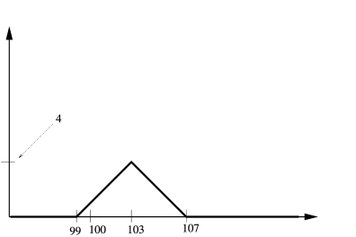
Figure 1: Butterfly spread payoff function used in the simulation.

As model for generating the stock values, we consider a $\operatorname{GARCH}(1,1)$ model in the form of Duan [4]. Here, we simulate the price process according to

$$X_{i+1} = X_{i}\cdot\exp\biggl{(}\frac{r^{*}}{4}-\frac{1}{2}\cdot\sigma_{i+1}^{2}+\sigma_{i+1}\cdot\varepsilon_{i+1}\biggr{)},$$

$$\sigma_{i+1}^{2} = \delta_{0}+\delta_{1}\cdot(\sigma_{i}\cdot\varepsilon_{i}-\lambda\cdot\sigma_{i})^{2}+\xi_{1}\cdot\sigma_{i}^{2},$$

where $r^{*}=0.05$, $\lambda=0.7136$, $\delta_{0}=0.0000664$, $\delta_{1}=0.144$, $\xi_{1}=0.776$ and where $(\varepsilon_{t})_{t\in\mathbb{Z}}$ are independent normally distributed random variables with expectation zero and variance one. We start our simulation with $X_{0}=x_{0}=100$. For $\sigma_{0}$, we use the random value we get if we start the second recursion with $\sigma^{2}_{-1600}=0$.

We consider four different algorithms to estimate the optimal stopping time: The first two algorithms are simple methods where we exercise the option at the first time when the payoff is greater than zero (simple1) or at the expiration date of the option (simple2). The third algorithm is the newly proposed algorithm of this article (new algorithm), and the fourth algorithm (optstop) is a regression-based Monte Carlo estimate of the optimal stopping rule based on the true price process, where we extend the state space in order to get a 3-dimensional Markovian process (i.e., we use $(X_{i},\sigma_{i},\varepsilon_{i})$ as variables of the algorithm). As regression-based Monte Carlo procedure, we use the smoothing spline algorithm described in Kohler [10], which gives results which are usually at least comparable but often better than the algorithms of Tsitsiklis and Van Roy [17] and Longstaff and Schwarz [14] based on parametric regression (cf. Kohler [11]). This algorithm can never be used in a real application since it requires that the distribution of the underlying data is known and since its decisions depend on the not observable random variables $\sigma_{i}$ and $\varepsilon_{i}$, however, it can be considered as an approximation of the theoretical optimal stopping rule.

In contrast to algorithms one and two, the algorithms three and four require training data. Our newly proposed algorithm three uses a path of values of length $1500$ (which is part of the path of length $1600$ preceding our evaluation paths) in order to learn its stopping rule, that is, it depends on observable values of the stock from the past. The theoretical algorithm four requires a training set consisting of paths generated independently and identically to the path for which it should generate the stopping rule (which is never available in any real application). In our simulation, the algorithm is based on $1000$ paths of length $5$ starting with $x_{0}=100$, each of them extending the same path before time $t_{0}=0$ used also in the evaluation of the stopping rule.

All algorithms are evaluated by applying them to $1000$ paths of length $5$ starting with $x_{0}=100$, where each of them extends the same path before time $t_{0}=0$, and we compute the average of the $1000$ payoffs achieved. Since for two of our four algorithms this result depends on the random training data, we repeat this whole procedure $100$ times and report the means and the standard deviations of the resulting values for each algorithm.

In the practical implementation of our newly proposed algorithm, we consider as bandwidths $h\in\{0.001,0.01,0.1\}$ and use the $k\in\{0,1,2\}$ last values of the returns for prediction of the value at the next time step. Each of these $3\cdot 3=9$ models gets the same probability $p_{k,r}=\frac{1}{9}$, and for the constant used for computing the weights of the estimate from the cumulative empirical losses we use $c=8B^{2}$ where $B$ is the maximal value of the payoff function. In addition, we make the following modifications: Firstly, we simplify the computation of the algorithm in such a way that we do not use the final averaging step (10), because otherwise we are not able to compute the result of our algorithm in a reasonable time on a standard computer. Secondly, we do not use returns relative to the previous day as $x$-values for our regression estimates, instead we use returns relative to the beginning of the time interval of an option. With the later modification, it can be shown that the theoretical result above is still valid because a consecutive sequence of these modified returns generates the same $\sigma$-algebra as the corresponding original returns. Finally, we ignore the first $n_{0,t}=(L-1-t)\cdot 200$ data points during the computation of $\hat{q}_{t}^{(n)}$ since we think that the first $n_{0,t}$ values of $\hat{q}_{t+1}^{(n)}$ are not reliable because they are based on too few data points.

The results of the four algorithms are reported in Table 1. As we can see from Table 1 both simple algorithms are clearly outperformed by our newly proposed algorithm, which achieves results which are very close to the results of the exercising strategy optstop relying on information not available in a real application.

Table 1: Achieved payoffs by the four different algorithms

	Simple1	Simple2	New algorithm	Optstop
Mean value	$\hphantom{(}1.00$	$\hphantom{(}0.61$	$\hphantom{(}1.64$	$\hphantom{(}1.72$
(Standard deviation)	$(0.00)$	$(0.04)$	$(0.47)$	$(0.04)$

From Table 1, we see that in principle our new algorithm could also be used as a numerical tool to evaluate American options as the algorithms of Tsitsiklis and Van Roy [17], Longstaff and Schwarz [14] or its nonparametric version used for optstop. However, it should be mentioned that our new algorithm needs much more time to compute its results: For one of the $100$ values computed for Table 1, it needs approximately $2$ hours as opposed to $4$ minutes needed by the optstop algorithm.

5 Proofs

5.1 Preliminaries to the proof of Theorem 3.1

Once we have constructed approximations $\hat{q}_{j}(z_{-\infty}^{j})$ of the continuation values $q_{j}(z_{-\infty}^{j})$, we can use them to construct an approximation

$$\hat{\tau}=\inf\bigl{\{}j\in\{0,1,\dots,L\}\colon\ g_{j}\bigl{(}Z_{1}^{j}\bigr{)}\geq\hat{q}_{j}\bigl{(}Z_{-\infty}^{j}\bigr{)}\bigr{\}}$$

of the optimal stopping time $\tau^{*}$.

As our next lemma shows, the errors of the estimates $\hat{q}_{j}$ determine the quality of the constructed stopping time.

Lemma 5.1

Assume $\hat{q}_{L}=0$. Then

$$\mathbf{E}\bigl{\{}g_{\tau^{*}}\bigl{(}Z_{1}^{\tau^{*}}\bigr{)}|Z_{-\infty}^{-1}\bigr{\}}-\mathbf{E}\bigl{\{}g_{\hat{\tau}}\bigl{(}Z_{1}^{\hat{\tau}}\bigr{)}|Z_{-\infty}^{-1}\bigr{\}}\leq\sum_{j=0}^{L-1}\mathbf{E}\bigl{\{}\bigl{|}\hat{q}_{j}\bigl{(}Z_{-\infty}^{j}\bigr{)}-q_{j}\bigl{(}Z_{-\infty}^{j}\bigr{)}\bigr{|}|Z_{-\infty}^{-1}\bigr{\}}.$$

The assertion follows from a modification of the proof of Proposition 21 in Belomestny [1]. For the sake of completeness, a complete proof is given in the Appendix.

5.2 Proof of Theorem 3.1

Stationarity of $(Z_{n})_{n\in\mathbb{Z}}$ implies that

$$Z_{-\infty}^{j}\mbox{ and }Z_{-\infty}^{j+l}\mbox{ have the same distribution for all }l\in\mathbb{Z}.$$ (11)

In the sequel, we want to bound

$$V_{0}-\hat{V}_{0,n} = \mathbf{E}\bigl{\{}g_{\tau^{*}}\bigl{(}Z_{1}^{\tau^{*}}\bigr{)}-g_{\hat{\tau}_{n}}\bigl{(}Z_{1}^{\hat{\tau}_{n}}\bigr{)}\bigr{\}}=\mathbf{E}\bigl{\{}\mathbf{E}\bigl{\{}g_{\tau^{*}}\bigl{(}Z_{1}^{\tau^{*}}\bigr{)}-g_{\hat{\tau}_{n}}\bigl{(}Z_{1}^{\hat{\tau}_{n}}\bigr{)}|Z_{-\infty}^{-1}\bigr{\}}\bigr{\}}.$$

By Lemma 5.1, we have

$$V_{0}-\hat{V}_{0,n}\leq\sum_{j=0}^{L-1}\mathbf{E}\bigl{\{}\bigl{|}\hat{q}_{j,n}\bigl{(}Z_{-n+1}^{j}\bigr{)}-q_{j}\bigl{(}Z_{-\infty}^{j}\bigr{)}\bigr{|}\bigr{\}},$$

so it suffices to show

$$\mathbf{E}\bigl{\{}\bigl{|}\hat{q}_{j,n}\bigl{(}Z_{-n+1}^{j}\bigr{)}-q_{j}\bigl{(}Z_{-\infty}^{j}\bigr{)}\bigr{|}\bigr{\}}\rightarrow 0\qquad(n\rightarrow\infty)$$ (12)

for $j\in\{0,1,\dots,L-1\}$.

Using the definition of $\hat{q}_{j,n}$ as arithmetic mean and the triangle inequality, we get

$$\mathbf{E}\bigl{\{}\bigl{|}\hat{q}_{j,n}\bigl{(}Z_{-n+1}^{j}\bigr{)}-q_{j}\bigl{(}Z_{-\infty}^{j}\bigr{)}\bigr{|}\bigr{\}} = \mathbf{E}\Biggl{\{}\Biggl{|}\frac{1}{n}\sum_{l=1}^{n}\hat{q}_{j}^{(l)}\bigl{(}Z_{-l+1}^{j}\bigr{)}-q_{j}\bigl{(}Z_{-\infty}^{j}\bigr{)}\Biggr{|}\Biggr{\}}$$

$$\leq \frac{1}{n}\sum_{l=1}^{n}\mathbf{E}\bigl{\{}\bigl{|}\hat{q}_{j}^{(l)}\bigl{(}Z_{-l+1}^{j}\bigr{)}-q_{j}\bigl{(}Z_{-\infty}^{j}\bigr{)}\bigr{|}\bigr{\}}$$

$$\stackrel{{\scriptstyle(\ref{se2eq8})}}{{=}} \frac{1}{n}\sum_{l=1}^{n}\mathbf{E}\bigl{\{}\bigl{|}\hat{q}_{j}^{(l)}\bigl{(}Z_{1}^{j+l}\bigr{)}-q_{j}\bigl{(}Z_{-\infty}^{j+l}\bigr{)}\bigr{|}\bigr{\}}$$

$$= \mathbf{E}\Biggl{\{}\frac{1}{n}\sum_{l=1}^{n}\bigl{|}\hat{q}_{j}^{(l)}\bigl{(}Z_{1}^{j+l}\bigr{)}-q_{j}\bigl{(}Z_{-\infty}^{j+l}\bigr{)}\bigr{|}\Biggr{\}}.$$

Because of the Cauchy–Schwarz inequality, it suffices to show

$$\mathbf{E}\Biggl{\{}\frac{1}{n}\sum_{l=1}^{n}\bigl{|}\hat{q}_{j}^{(l)}\bigl{(}Z_{1}^{j+l}\bigr{)}-q_{j}\bigl{(}Z_{-\infty}^{j+l}\bigr{)}\bigr{|}^{2}\Biggr{\}}\rightarrow 0$$ (13)

$(n\rightarrow\infty)$ for all $j\in\{0,\dots,L-1\}$. And because of boundedness of the estimates and of $q_{j}$ this in turn follows from

$$\frac{1}{n}\sum_{l=1}^{n}\bigl{|}\hat{q}_{j}^{(l)}\bigl{(}Z_{1}^{j+l}\bigr{)}-q_{j}\bigl{(}Z_{-\infty}^{j+l}\bigr{)}\bigr{|}^{2}\rightarrow 0$$ (14)

in probability for all $j\in\{0,\dots,L-1\}$.

The idea is now to use techniques from Section 27.5 (in particular Corollary 27.1) in Györfi et al. [7]. We have in mind definitions (2), (2) and (9), also $\hat{q}_{L}^{(n)}:=0$, and define estimates $\hat{m}_{j}^{(n)}(z_{1}^{n},\cdot)$ of $m_{j}:=q_{j}$ using realizations $z_{1},\dots,z_{n}$ of $Z_{1}$, …, $Z_{n}$, with arguments $u_{1}$, …, $u_{n+j}$. We start with

$$\hat{m}_{L}^{(n)}\bigl{(}z_{1}^{n};\cdot\bigr{)}:=0.$$

Given $\hat{m}^{(n)}_{j+1}(z_{1}^{n};\cdot)$ for $j\in\{0,1,\dots,L-1\}$ we define $\hat{m}^{(n)}_{j}(z_{1}^{n};\cdot)$ as follows.

We start with defining $\hat{m}_{j,n,(k,h)}(z_{1}^{n};\cdot)$ with parameters $k\in\mathbb{N}$ and $h>0$ using local averaging (around $u_{1}^{n+j}$) by

$$\hat{m}_{j,n,(k,h)}\bigl{(}z_{1}^{n};u_{1}^{n+j}\bigr{)}$$

$$\quad:=\sum_{i=k+1}^{n-j-1}\max\bigl{\{}g_{j+1}\bigl{(}z_{i+1}^{i+j+1}\bigr{)},\hat{m}_{j+1}^{(i)}\bigl{(}z_{1}^{i};z_{1}^{i+j+1}\bigr{)}\bigr{\}}$$ (15)

$$\hskip 48.0pt{}\cdot{K\biggl{(}\frac{u_{n-k}^{n+j}-z_{i-k}^{i+j}}{h}\biggr{)}}\bigg{/}{\sum_{l=k+1}^{n-j-1}K\biggl{(}\frac{u_{n-k}^{n+j}-z_{l-k}^{l+j}}{h}\biggr{)}}.$$

Here we set

$$\hat{m}_{j,n,(k,h)}\bigl{(}z_{1}^{n};\cdot\bigr{)}:=0$$

for $k\geq n-j-1$.

For $(k,h)\in\mathcal{P}$ (where $\mathcal{P}$ is the parameter set in the definition of the estimate), define the cumulative loss of the estimate with parameter $(k,h)$ by

$$\hat{L}_{n,j}(k,h) := \hat{L}_{n,j}\bigl{(}k,h;z_{1}^{n-1};u_{1}^{n+j}\bigr{)}$$

$$\hskip 2.8pt= \frac{1}{n}\sum_{i=1}^{n-1}\bigl{(}\hat{m}_{j,i,(k,h)}\bigl{(}z_{1}^{i};u_{1}^{i+j}\bigr{)}-\max\bigl{\{}g_{j+1}\bigl{(}u_{i+1}^{i+j+1}\bigr{)},\hat{m}_{j+1}^{(i)}\bigl{(}z_{1}^{i};u_{1}^{i+j+1}\bigr{)}\bigr{\}}\bigr{)}^{2}.$$

Put $c:=8B^{2}$ (where $B$ is the bound on the gain functions), let $(p_{k,r})_{k,r}$ be the probability distribution used in the definition of the estimate (which satisfies $p_{k,r}>0$ for all $k,r\in\mathbb{N}$) and define weights, which depend on these cumulative losses, by

$$w_{n,k,r}^{(j)}:=w_{n,k,r}^{(j)}\bigl{(}z_{1}^{n-1};u_{1}^{n+j}\bigr{)}=p_{k,r}\cdot\mathrm{e}^{-n\hat{L}_{n,j}(k,h_{r})/c}$$

and their normalized values by

$$v_{n,k,r}^{(j)}:=v_{n,k,r}^{(j)}\bigl{(}z_{1}^{n-1};u_{1}^{n+j}\bigr{)}=\frac{w_{n,k,r}^{(j)}}{\sum_{s,t=1}^{\infty}w_{n,s,t}^{(j)}}.$$

The estimate $\hat{m}_{j}^{(n)}$ is defined as the convex combination of all estimates $\hat{m}_{j,n,(k,h_{r})}$ using weights $v_{n,k,r}^{(j)}$, that is, $\hat{m}_{j}^{(n)}$ is defined by

$$\hat{m}_{j}^{(n)}\bigl{(}z_{1}^{n};u_{1}^{n+j}\bigr{)}:=\sum_{k,r=1}^{\infty}v_{n,k,r}^{(j)}\cdot\hat{m}_{j,n,(k,h_{r})}\bigl{(}z_{1}^{n};u_{1}^{n+j}\bigr{)}.$$

By using a backward induction with respect to $j$ starting with $L$, it is easy to see that we have

$$\hat{m}_{j,(k,h)}^{(n)}=\hat{m}_{j,n,(k,h)},\qquad\hat{q}_{j}^{(n)}\bigl{(}z_{-n+1}^{j}\bigr{)}=\hat{m}^{(n)}_{j}\bigl{(}z_{-n+1}^{0};z_{-n+1}^{j}\bigr{)},$$

further

$$\hat{Q}_{n,j}(k,h)=\hat{Q}_{n,j}\bigl{(}z_{-n+1}^{j},k,h\bigr{)}=\hat{L}_{n,j}\bigl{(}k,h;z_{-n+1}^{-1};z_{-n+1}^{j}\bigr{)}.$$

Thus, (14) means

$$\frac{1}{n}\sum_{l=1}^{n}\bigl{|}\hat{m}_{t}^{(l)}\bigl{(}Z_{1}^{l};Z_{1}^{l+t}\bigr{)}-m_{t}\bigl{(}Z_{-\infty}^{l+t}\bigr{)}\bigr{|}^{2}\rightarrow 0$$ (16)

in probability for all $t\in\{0,1,\dots,L\}$, which we show by backward induction with respect to $t$.

We start with $t=L$ in which the assertion is trivial since

$$\hat{m}^{(l)}_{L}=0\quad\mbox{and}\quad m_{L}=0$$

for all $l\in\mathbb{N}$.

Assume now that (16) holds for $t=j+1$ for some $j\in\{0,1,\dots,L-1\}$. We have to show that in this case it is also valid for $t=j$.

Set

$$L_{n}(\hat{m}_{j}) := \frac{1}{n}\sum_{l=1}^{n-1}\bigl{|}\hat{m}_{j}^{(l)}\bigl{(}Z_{1}^{l};Z_{1}^{l+j}\bigr{)}-\max\bigl{\{}g_{j+1}\bigl{(}Z_{l+1}^{l+j+1}\bigr{)},m_{j+1}\bigl{(}Z_{-\infty}^{l+j+1}\bigr{)}\bigr{\}}\bigr{|}^{2},$$

$$L_{n}(\hat{m}_{j,\cdot,(k,h)}) := \frac{1}{n}\sum_{l=1}^{n-1}\bigl{|}\hat{m}_{j,l,(k,h)}\bigl{(}Z_{1}^{l};Z_{1}^{l+j}\bigr{)}-\max\bigl{\{}g_{j+1}\bigl{(}Z_{l+1}^{l+j+1}\bigr{)},m_{j+1}\bigl{(}Z_{-\infty}^{l+j+1}\bigr{)}\bigr{\}}\bigr{|}^{2},$$

$$\hat{L}_{n}(\hat{m}_{j}) := \frac{1}{n}\sum_{l=1}^{n-1}\bigl{|}\hat{m}_{j}^{(l)}\bigl{(}Z_{1}^{l};Z_{1}^{l+j}\bigr{)}-\max\bigl{\{}g_{j+1}\bigl{(}Z_{l+1}^{l+j+1}\bigr{)},\hat{m}_{j+1}^{(l)}\bigl{(}Z_{1}^{l};Z_{1}^{l+j+1}\bigr{)}\bigr{\}}\bigr{|}^{2}$$

and

$$\hat{L}_{n}(\hat{m}_{j,\cdot,(k,h)}) := \hat{L}_{n,j}\bigl{(}k,h;Z_{1}^{n-1};Z_{1}^{n+j}\bigr{)}$$

$$:= \frac{1}{n}\sum_{l=1}^{n-1}\bigl{|}\hat{m}_{j,l,(k,h)}\bigl{(}Z_{1}^{l};Z_{1}^{l+j}\bigr{)}-\max\bigl{\{}g_{j+1}\bigl{(}Z_{l+1}^{l+j+1}\bigr{)},\hat{m}_{j+1}^{(l)}\bigl{(}Z_{1}^{l};Z_{1}^{l+j+1}\bigr{)}\bigr{\}}\bigr{|}^{2}.$$

By Lemma 27.3 in Györfi et al. [7], we get

$$\hat{L}_{n}(\hat{m}_{j})\leq\inf_{k,r\in\mathbb{N}}\biggl{(}\hat{L}_{n}(\hat{m}_{j,\cdot,(k,h_{r})})-c\cdot\frac{\ln p_{k,r}}{n}\biggr{)}.$$ (17)

Set

$$L_{j}^{*}:=\mathbf{E}\bigl{\{}\bigl{|}m_{j}\bigl{(}Z_{-\infty}^{j}\bigr{)}-\max\bigl{\{}g_{j+1}\bigl{(}Z_{1}^{j+1}\bigr{)},m_{j+1}\bigl{(}Z_{-\infty}^{j+1}\bigr{)}\bigr{\}}\bigr{|}^{2}\bigr{\}}.$$

In order to show (16), we use the following lemma which we prove directly after the end of this proof.

Lemma 5.2

Let $j\in\{0,\dots,L-1\}$. If (16) holds for $t=j+1$, then

$$L_{n}(\hat{m}_{j})\rightarrow L_{j}^{*}\qquad\mbox{in probability.}$$ (18)

We use (18) to show (16) for $t=j$. To do this, we proceed as in the proof of Corollary 27.1 in Györfi et al. [7]. Consider the following decomposition:

$$\bigl{(}\hat{m}_{j}^{(l)}\bigl{(}Z_{1}^{l};Z_{1}^{l+j}\bigr{)}-\max\bigl{\{}g_{j+1}\bigl{(}Z_{l+1}^{l+j+1}\bigr{)},m_{j+1}\bigl{(}Z_{-\infty}^{l+j+1}\bigr{)}\bigr{\}}\bigr{)}^{2}$$

$$\quad=\bigl{(}\hat{m}_{j}^{(l)}\bigl{(}Z_{1}^{l};Z_{1}^{l+j}\bigr{)}-m_{j}\bigl{(}Z_{-\infty}^{l+j}\bigr{)}\bigr{)}^{2}+\bigl{(}m_{j}\bigl{(}Z_{-\infty}^{l+j}\bigr{)}-\max\bigl{\{}g_{j+1}\bigl{(}Z_{l+1}^{l+j+1}\bigr{)},m_{j+1}\bigl{(}Z_{-\infty}^{l+j+1}\bigr{)}\bigr{\}}\bigr{)}^{2}$$

$$\qquad{}+2\cdot\bigl{(}\hat{m}_{j}^{(l)}\bigl{(}Z_{1}^{l};Z_{1}^{l+j}\bigr{)}-m_{j}\bigl{(}Z_{-\infty}^{l+j}\bigr{)}\bigr{)}$$

$$\qquad\quad{}\cdot\bigl{(}m_{j}\bigl{(}Z_{-\infty}^{l+j}\bigr{)}-\max\bigl{\{}g_{j+1}\bigl{(}Z_{l+1}^{l+j+1}\bigr{)},m_{j+1}\bigl{(}Z_{-\infty}^{l+j+1}\bigr{)}\bigr{\}}\bigr{)}.$$

By (18), we know

$$\frac{1}{n}\sum_{l=1}^{n}\bigl{(}\hat{m}_{j}^{(l)}\bigl{(}Z_{1}^{l};Z_{1}^{l+j}\bigr{)}-\max\bigl{\{}g_{j+1}\bigl{(}Z_{l+1}^{l+j+1}\bigr{)},m_{j+1}\bigl{(}Z_{-\infty}^{l+j+1}\bigr{)}\bigr{\}}\bigr{)}^{2}\rightarrow L_{j}^{*}$$

in probability. Furthermore, by the ergodic theorem we have

$$\frac{1}{n}\sum_{l=1}^{n}\bigl{(}m_{j}\bigl{(}Z_{-\infty}^{l+j}\bigr{)}-\max\bigl{\{}g_{j+1}\bigl{(}Z_{l+1}^{l+j+1}\bigr{)},m_{j+1}\bigl{(}Z_{-\infty}^{l+j+1}\bigr{)}\bigr{\}}\bigr{)}^{2}\rightarrow L_{j}^{*}\qquad\mbox{a.s.}$$

Hence, it suffices to show

$$\frac{1}{n}\sum_{l=1}^{n}\bigl{(}\hat{m}_{j}^{(l)}\bigl{(}Z_{1}^{l};Z_{1}^{l+j}\bigr{)}-m_{j}\bigl{(}Z_{-\infty}^{l+j}\bigr{)}\bigr{)}$$

$$\hskip 24.0pt{}\cdot\bigl{(}m_{j}\bigl{(}Z_{-\infty}^{l+j}\bigr{)}-\max\bigl{\{}g_{j+1}\bigl{(}Z_{l+1}^{l+j+1}\bigr{)},m_{j+1}\bigl{(}Z_{-\infty}^{l+j+1}\bigr{)}\bigr{\}}\bigr{)}$$ (19)

$$\quad\rightarrow 0\qquad\mbox{a.s.}$$

The random variables

$$\bigl{(}\hat{m}_{j}^{(l)}\bigl{(}Z_{1}^{l};Z_{1}^{l+j}\bigr{)}-m_{j}\bigl{(}Z_{-\infty}^{l+j}\bigr{)}\bigr{)}\cdot\bigl{(}m_{j}\bigl{(}Z_{-\infty}^{l+j}\bigr{)}-\max\bigl{\{}g_{j+1}\bigl{(}Z_{l+1}^{l+j+1}\bigr{)},m_{j+1}\bigl{(}Z_{-\infty}^{l+j+1}\bigr{)}\bigr{\}}\bigr{)}$$

are martingale differences because of $m_{j}=q_{j}$, (5), stationarity and dependence of the first factor on $Z_{-\infty}^{l+j}$ (not on $Z_{-\infty}^{l+j+1}$), and they are bounded by $4B^{2}$. Therefore (5.2) is a consequence of Theorem A.6 in Györfi et al. [7] (which we apply with $c_{i}=1$).

5.3 Proof of Lemma 5.2

By $|\max\{a,b\}-\max\{a,c\}|\leq|b-c|$ $(a,b,c\in\mathbb{R})$ and (16) for $t=j+1$, we get

$$\frac{1}{n}\sum_{l=1}^{n-1}\bigl{|}\max\bigl{\{}g_{j+1}\bigl{(}Z_{l+1}^{l+j+1}\bigr{)},m_{j+1}\bigl{(}Z_{-\infty}^{l+j+1}\bigr{)}\bigr{\}}$$

$$\hskip 25.0pt{}-\max\bigl{\{}g_{j+1}\bigl{(}Z_{l+1}^{l+j+1}\bigr{)},\hat{m}_{j+1}^{(l)}\bigl{(}Z_{1}^{l};Z_{1}^{l+j+1}\bigr{)}\bigr{\}}\bigr{|}^{2}$$

$$\quad\leq\frac{1}{n}\sum_{l=1}^{n-1}\bigl{|}\hat{m}_{j+1}^{(l)}\bigl{(}Z_{1}^{l};Z_{1}^{l+j+1}\bigr{)}-m_{j+1}\bigl{(}Z_{-\infty}^{l+j+1}\bigr{)}\bigr{|}^{2}$$

$$\quad\rightarrow 0\qquad\mbox{in probability.}$$

Using

$$\frac{1}{n}\sum_{l=1}^{n-1}|a_{l}-b_{l}|^{2}-\frac{1}{n}\sum_{l=1}^{n-1}|a_{l}-c_{l}|^{2}$$

$$\quad=\frac{1}{n}\sum_{l=1}^{n-1}(a_{l}-b_{l}+a_{l}-c_{l})\cdot(c_{l}-b_{l})$$

$$\quad\leq\Biggl{(}\frac{1}{n}\sum_{l=1}^{n-1}(a_{l}-b_{l}+a_{l}-c_{l})^{2}\Biggr{)}^{1/2}\cdot\Biggl{(}\frac{1}{n}\sum_{l=1}^{n-1}(c_{l}-b_{l})^{2}\Biggr{)}^{1/2}$$

and the boundedness of the gain functions we see that this implies

$$L_{n}(\hat{m}_{j})-\hat{L}_{n}(\hat{m}_{j})\rightarrow 0\quad\mbox{and}\quad L_{n}(\hat{m}_{j,\cdot,(k,h)})-\hat{L}_{n}(\hat{m}_{j,\cdot,(k,h)})\rightarrow 0$$ (20)

in probability. Hence for an arbitrary subsequence $(n_{l})_{l}$ of $(n)_{n}$, we find a subsubsequence $(n_{l_{s}})_{s}$ of $(n_{l})_{l}$ such that we have with probability one

$$\mathop{\lim\sup}_{s\rightarrow\infty}L_{n_{l_{s}}}(\hat{m}_{j}) = \mathop{\lim\sup}_{s\rightarrow\infty}\hat{L}_{n_{l_{s}}}(\hat{m}_{j})$$

$$\stackrel{{\scriptstyle(\ref{pth1eq4})}}{{\leq}} \mathop{\lim\sup}_{s\rightarrow\infty}\inf_{k,r\in\mathbb{N}}\biggl{(}\hat{L}_{n_{l_{s}}}(\hat{m}_{j,\cdot,(k,h_{r})})-c\cdot\frac{\ln p_{k,r}}{n_{l_{s}}}\biggr{)}$$

$$\leq \inf_{k,r\in\mathbb{N}}\mathop{\lim\sup}_{s\rightarrow\infty}\biggl{(}\hat{L}_{n_{l_{s}}}(\hat{m}_{j,\cdot,(k,h_{r})})-c\cdot\frac{\ln p_{k,r}}{n_{l_{s}}}\biggr{)}$$

$$= \inf_{k,r\in\mathbb{N}}\mathop{\lim\sup}_{s\rightarrow\infty}L_{n_{l_{s}}}(\hat{m}_{j,\cdot,(k,h_{r})}).$$

Of course, this relation also holds if we replace $(n_{l_{s}})_{s}$ by any of its subsequences (which we will do later in the proof).

Next, we analyze $L_{n}(\hat{m}_{j,\cdot,(k,h_{r})})$. According to (5.2), we have

$$\hat{m}_{j,n,(k,h)}\bigl{(}Z_{1}^{n};v_{-n+1}^{j}\bigr{)}$$

$$\quad={\sum_{i=k+1}^{n-j-1}\max\bigl{\{}g_{j+1}\bigl{(}Z_{i+1}^{i+j+1}\bigr{)},\hat{m}_{j+1}^{(i)}\bigl{(}Z_{1}^{i};Z_{1}^{i+j+1}\bigr{)}\bigr{\}}\cdot K\biggl{(}\frac{v_{-k}^{j}-Z_{i-k}^{i+j}}{h}\biggr{)}}$$

$$\qquad\bigg{/}{\sum_{i=k+1}^{n-j-1}K\biggl{(}\frac{v_{-k}^{j}-Z_{i-k}^{i+j}}{h}\biggr{)}}$$

$$\quad=\frac{A_{n}}{C_{n}}+\frac{B_{n}-A_{n}}{C_{n}},$$

where

$$A_{n} := \frac{1}{n-j-k-1}\sum_{i=k+1}^{n-j-1}\max\bigl{\{}g_{j+1}\bigl{(}Z_{i+1}^{i+j+1}\bigr{)},m_{j+1}\bigl{(}Z_{-\infty}^{i+j+1}\bigr{)}\bigr{\}}\cdot K\biggl{(}\frac{v_{-k}^{j}-Z_{i-k}^{i+j}}{h}\biggr{)},$$

$$B_{n} := \frac{1}{n-j-k-1}\sum_{i=k+1}^{n-j-1}\max\bigl{\{}g_{j+1}\bigl{(}Z_{i+1}^{i+j+1}\bigr{)},\hat{m}_{j+1}^{(i)}\bigl{(}Z_{1}^{i};Z_{1}^{i+j+1}\bigr{)}\bigr{\}}\cdot K\biggl{(}\frac{v_{-k}^{j}-Z_{i-k}^{i+j}}{h}\biggr{)}$$

and

$$C_{n}:=\frac{1}{n-j-k-1}\sum_{i=k+1}^{n-j-1}K\biggl{(}\frac{v_{-k}^{j}-Z_{i-k}^{i+j}}{h}\biggr{)}.$$

By the ergodic theorem, we get

$$A_{n}\rightarrow\mathbf{E}\biggl{\{}\max\bigl{\{}g_{j+1}\bigl{(}Z_{1}^{j+1}\bigr{)},m_{j+1}\bigl{(}Z_{-\infty}^{j+1}\bigr{)}\bigr{\}}\cdot K\biggl{(}\frac{v_{-k}^{j}-Z_{-k}^{j}}{h}\biggr{)}\biggr{\}}\qquad\mbox{a.s.}$$

and

$$C_{n}\rightarrow\mathbf{E}\biggl{\{}K\biggl{(}\frac{v_{-k}^{j}-Z_{-k}^{j}}{h}\biggr{)}\biggr{\}}\qquad\mbox{a.s.}$$

If we use the continuity of the kernel function, we can even apply an ergodic theorem in the separable Banach space of continuous functions vanishing at infinity (with supremum norm) and get that the almost sure convergence of $A_{n}$ and $C_{n}$ is uniformly with respect to $v_{-k}^{j}$ (cf., e.g., Krengel [12], Chapter 4, Theorem 2.1).

Furthermore, using the triangle inequality,

$$\bigl{|}\max\{a,b\}-\max\{a,c\}\bigr{|}\leq|b-c|\qquad(a,b,c\in\mathbb{R}),$$

and the Cauchy–Schwarz inequality we can conclude

$$|B_{n}-A_{n}| \leq \frac{1}{n-j-k-1}\sum_{i=k+1}^{n-j-1}\bigl{|}\hat{m}_{j+1}^{(i)}\bigl{(}Z_{1}^{i};Z_{1}^{i+j+1}\bigr{)}-m_{j+1}\bigl{(}Z_{-\infty}^{i+j+1}\bigr{)}\bigr{|}\cdot K\biggl{(}\frac{v_{-k}^{j}-Z_{i-k}^{i+j}}{h}\biggr{)}$$

$$\leq \sqrt{\frac{1}{n-j-k-1}\sum_{i=k+1}^{n-j-1}\bigl{|}\hat{m}_{j+1}^{(i)}\bigl{(}Z_{1}^{i};Z_{1}^{i+j+1}\bigr{)}-m_{j+1}\bigl{(}Z_{-\infty}^{i+j+1}\bigr{)}\bigr{|}^{2}}$$

$${}\cdot\sqrt{\frac{1}{n-j-k-1}\sum_{i=k+1}^{n-j-1}K\biggl{(}\frac{v_{-k}^{j}-Z_{i-k}^{i+j}}{h}\biggr{)}^{2}}.$$

By the ergodic theorem, the second factor on the right-hand side above converges to

$$\sqrt{\mathbf{E}\biggl{\{}K\biggl{(}\frac{v_{-k}^{j}-Z_{-k}^{j}}{h}\biggr{)}^{2}\biggr{\}}}<\infty$$

with probability one (where we have again uniform convergence with respect to $v_{-k}^{j}$), and the first factor converges in probability to zero by (16) for $t=j+1$. Because of $K\geq c\cdot I_{S_{0,r}}$ for suitable $c>0$, $r>0$, where $S_{0,r}$ is the ball in $\mathbb{R}^{j+k+1}$ centered at $0$ with radius $r$, we have

$$\mathbf{E}\biggl{\{}K\biggl{(}\frac{v_{-k}^{j}-Z_{-k}^{j}}{h}\biggr{)}\biggr{\}}\geq c\cdot\mathbf{P}_{Z_{-k}^{j}}\bigl{(}v_{-k}^{j}+S_{0,r\cdot h}\bigr{)}>0\qquad\mathbf{P}_{Z_{-k}^{j}}\!\mbox{-almost everywhere}$$ (22)

(cf., e.g., Györfi et al. [7], pages 499, 500). (If $K>0$ everywhere, then (22) also holds everywhere.) Therefore,

$$\frac{B_{n}-A_{n}}{C_{n}}\rightarrow 0\qquad\mbox{in probability }\mathbf{P}_{Z_{-k}^{j}}\!\mbox{-almost everywhere},$$

from which we get

$$\hat{m}_{j,n,(k,h)}\bigl{(}Z_{1}^{n};v_{-n+1}^{j}\bigr{)}\rightarrow m_{j,(k,h)}\bigl{(}v_{-k}^{j}\bigr{)}\qquad\mbox{in probability}$$

$\mathbf{P}_{Z_{-k}^{j}}$-almost everywhere, where

$$m_{j,(k,h)}(v_{-k},\dots,v_{j})$$

$$\quad={\mathbf{E}\biggl{\{}\max\bigl{\{}g_{j+1}\bigl{(}Z_{1}^{j+1}\bigr{)},m_{j+1}\bigl{(}Z_{-\infty}^{j+1}\bigr{)}\bigr{\}}\cdot K\biggl{(}\frac{Z_{-k}^{j}-v_{-k}^{j}}{h}\biggr{)}\biggr{\}}}\bigg{/}{\mathbf{E}\biggl{\{}K\biggl{(}\frac{Z_{-k}^{j}-v_{-k}^{j}}{h}\biggr{)}\biggr{\}}}.$$

Let $\varepsilon>0$ be arbitrary and set

$$S_{\varepsilon}=\biggl{\{}v_{-k}^{j}\in\mathbb{R}^{k+j+1}\colon\ \mathbf{E}\biggl{\{}K\biggl{(}\frac{v_{-k}^{j}-Z_{-k}^{j}}{h}\biggr{)}\biggr{\}}>\varepsilon\biggr{\}}.$$

By (22), we know

$$\mathbf{P}_{Z_{-k}^{j}}(S_{\varepsilon})\rightarrow 1\qquad(\varepsilon\rightarrow 0).$$

Since the numerators and the denominators above converge uniformly with respect to $v_{-k}^{j}$ and since the limit of the denominators is greater than $\varepsilon$ on $S_{\varepsilon}$, we know in addition

$$\sup_{v_{-n+1},\dots,v{-k-1}\in\mathbb{R},v_{-k}^{j}\in S_{\varepsilon}}\bigl{|}\hat{m}_{j,n,(k,h)}\bigl{(}Z_{1}^{n};v_{-n+1}^{j}\bigr{)}-m_{j,(k,h)}\bigl{(}v_{-k}^{j}\bigr{)}\bigr{|}\rightarrow 0$$ (23)

in probability. In the sequel, we want to use this to show

$$L_{n,j}(\hat{m}_{j,\cdot,(k,h)})$$

$$\quad=\frac{1}{n}\sum_{i=1}^{n-1}\bigl{(}\hat{m}_{j,i,(k,h)}\bigl{(}Z_{1}^{i};Z_{1}^{i+j}\bigr{)}-\max\bigl{\{}g_{j+1}\bigl{(}Z_{i+1}^{i+j+1}\bigr{)},m_{j+1}\bigl{(}Z_{-\infty}^{i+j+1}\bigr{)}\bigr{\}}\bigr{)}^{2}$$ (24)

$$\quad\rightarrow\mathbf{E}\bigl{\{}\bigl{|}m_{j,(k,h)}\bigl{(}Z_{-k}^{j}\bigr{)}-\max\bigl{\{}g_{j+1}\bigl{(}Z_{1}^{j+1}\bigr{)},m_{j+1}\bigl{(}Z_{-\infty}^{j+1}\bigr{)}\bigr{\}}\bigr{|}^{2}\bigr{\}}$$

in probability. To do this, we observe first that the ergodic theorem implies

$$L_{n,j}(m_{j,(k,h)})$$

$$\quad=\frac{1}{n}\sum_{i=1}^{n-1}\bigl{(}m_{j,(k,h)}\bigl{(}Z_{i-k}^{i+j}\bigr{)}-\max\bigl{\{}g_{j+1}\bigl{(}Z_{i+1}^{i+j+1}\bigr{)},m_{j+1}\bigl{(}Z_{-\infty}^{i+j+1}\bigr{)}\bigr{\}}\bigr{)}^{2}$$

$$\quad\rightarrow\mathbf{E}\bigl{\{}\bigl{|}m_{j,(k,h)}\bigl{(}Z_{-k}^{j}\bigr{)}-\max\bigl{\{}g_{j+1}\bigl{(}Z_{1}^{j+1}\bigr{)},m_{j+1}\bigl{(}Z_{-\infty}^{j+1}\bigr{)}\bigr{\}}\bigr{|}^{2}\bigr{\}}$$

almost surely. Because of boundedness of the payoff function, we have in addition

$$\bigl{|}L_{n,j}(\hat{m}_{j,\cdot,(k,h)})-L_{n,j}(m_{j,(k,h)})\bigr{|}$$

$$\quad\leq c_{1}\cdot\frac{1}{n}\sum_{i=1}^{n-1}\bigl{|}\hat{m}_{j,i,(k,h)}\bigl{(}Z_{1}^{i};Z_{1}^{i+j}\bigr{)}-m_{j,(k,h)}\bigl{(}Z_{i-k}^{i+j}\bigr{)}\bigr{|}$$

$$\quad\leq c_{2}\cdot\frac{1}{n}\sum_{i=1}^{n-1}I_{S_{\varepsilon}^{c}}\bigl{(}Z_{i-k}^{i+j}\bigr{)}$$

$$\qquad{}+c_{1}\cdot\frac{1}{n}\sum_{i=1}^{n-1}\sup_{v_{-i+1},\dots,v_{-k-1}\in\mathbb{R},v_{-k}^{j}\in S_{\varepsilon}}\bigl{|}\hat{m}_{j,i,(k,h)}\bigl{(}Z_{1}^{i};v_{-i+1}^{j}\bigr{)}-m_{j,(k,h)}\bigl{(}v_{-k}^{j}\bigr{)}\bigr{|}$$

$$\quad\rightarrow c_{2}\cdot\mathbf{P}_{Z_{-k}^{j}}\bigl{(}S_{\varepsilon}^{c}\bigr{)}$$

in probability by (23) and by the ergodic theorem. By letting $\varepsilon\rightarrow 0$, we get (5.3). And by replacing $(n_{l_{s}})$ by a suitable subsequence of $(n_{l_{s}})_{s}$, we can assume w.l.o.g. even that (5.3) holds for almost sure convergence if we replace $n$ by $n_{l_{s}}$ in (5.3).

Next, we use Lemma 24.8 in Györfi et al. [7] which implies

$$m_{j,(k,h)}\bigl{(}z_{-k}^{j}\bigr{)}\rightarrow m_{j,k}\bigl{(}z_{-k}^{j}\bigr{)}\qquad\mathbf{P}_{Z_{-k}^{j}}\!\mbox{-almost everywhere}$$

for $h\rightarrow 0$, where

$$m_{j,k}\bigl{(}z_{-k}^{j}\bigr{)}:=\mathbf{E}\bigl{\{}\max\bigl{\{}g_{j+1}\bigl{(}Z_{1}^{j+1}\bigr{)},m_{j+1}\bigl{(}Z_{-\infty}^{j+1}\bigr{)}\bigr{\}}|Z_{-k}^{j}=z_{-k}^{j}\bigr{\}}.$$

And by the martingale convergence theorem, we have

$$m_{j,k}\bigl{(}Z_{-k}^{j}\bigr{)}\rightarrow m_{j}\bigl{(}Z_{-\infty}^{j}\bigr{)}\qquad\mbox{a.s.}$$

for $k\rightarrow\infty$ (since the almost sure limit $X$ of the left-hand side satisfies

$$\int_{A}X\,\mathrm{d}P=\int_{A}m_{j}\bigl{(}Z_{-\infty}^{j}\bigr{)}\,\mathrm{d}P$$

for all $A\in\mathcal{F}(Z_{-k}^{j})$ and all $k\in\mathbb{N}$, cf., e.g., Chapter 32.4A in Loève [13] for more general results in this respect). From this, we conclude by dominated convergence

$$\mathop{\lim\sup}_{s\rightarrow\infty}L_{n_{l_{s}}}(\hat{m}_{j})$$

$$\quad\stackrel{{\scriptstyle(\ref{pth1eq5})}}{{\leq}}\inf_{k,r\in\mathbb{N}}\mathop{\lim\sup}_{s\rightarrow\infty}L_{n_{l_{s}}}(\hat{m}_{j,\cdot,(k,h_{r})})$$

$$\quad\stackrel{{\scriptstyle(\ref{pth1eq7})}}{{=}}\inf_{k,r\in\mathbb{N}}\mathbf{E}\bigl{\{}\bigl{|}m_{j,(k,h_{r})}\bigl{(}Z_{-k}^{j}\bigr{)}-\max\bigl{\{}g_{j+1}\bigl{(}Z_{1}^{j+1}\bigr{)},m_{j+1}\bigl{(}Z_{-\infty}^{j+1}\bigr{)}\bigr{\}}\bigr{|}^{2}\bigr{\}}$$

$$\quad\leq L_{j}^{*}\qquad\mbox{a.s.}$$

Because of

$$\mathop{\lim\inf}_{n\rightarrow\infty}L_{n}(\hat{m}_{j})\geq L_{j}^{*}\qquad\mbox{a.s.}$$

(cf., e.g., Section 27.5 in Györfi et al. [7]) this completes the proof of (18).

Appendix: Proof of Lemma 5.1

Set

$$\hat{\tau}_{t}^{*}=\inf\bigl{\{}s\geq t+1\colon\ \hat{q}_{s}\bigl{(}Z_{-\infty}^{s}\bigr{)}\leq g_{s}\bigl{(}Z_{1}^{s}\bigr{)}\bigr{\}}$$

and let $\mathcal{F}_{t}$ be the $\sigma$-algebra generated by $Z_{-\infty}^{t}$. In the sequel, we prove

$$\mathbf{E}\bigl{\{}g_{\tau_{t-1}^{*}}\bigl{(}Z_{1}^{\tau_{t-1}^{*}}\bigr{)}-g_{\hat{\tau}^{*}_{t-1}}\bigl{(}Z_{1}^{\hat{\tau}^{*}_{t-1}}\bigr{)}|\mathcal{F}_{t-1}\bigr{\}}\leq\sum_{k=t}^{L-1}\mathbf{E}\bigl{\{}\bigl{|}\hat{q}_{k}\bigl{(}Z_{-\infty}^{k}\bigr{)}-q_{k}\bigl{(}Z_{-\infty}^{k}\bigr{)}\bigr{|}|\mathcal{F}_{t-1}\bigr{\}}\quad$$ (1)

for $t\in\{0,\dots,L\}$, from which we get the assertion of Lemma 5.1 by setting $t=0$.

We prove (1) by induction. The assertion is trivial for $t=L$ (since $\tau_{L-1}^{*}=L=\hat{\tau}^{*}_{L-1}$). Assume that (1) holds for $t\in\{s+1,\dots,L\}$ for some $s\in\{0,1,\dots,L-1\}$. In the sequel we prove that in this case it also holds for $t=s$. To do this, we use

$$\mathbf{E}\bigl{\{}g_{\tau_{t-1}^{*}}\bigl{(}Z_{1}^{\tau_{t-1}^{*}}\bigr{)}-g_{\hat{\tau}^{*}_{t-1}}\bigl{(}Z_{1}^{\hat{\tau}^{*}_{t-1}}\bigr{)}|\mathcal{F}_{t-1}\bigr{\}}$$

$$\quad=\sum_{k=t}^{L-1}\mathbf{E}\bigl{\{}\bigl{(}g_{\tau_{t-1}^{*}}\bigl{(}Z_{1}^{\tau_{t-1}^{*}}\bigr{)}-g_{\hat{\tau}^{*}_{t-1}}\bigl{(}Z_{1}^{\hat{\tau}^{*}_{t-1}}\bigr{)}\bigr{)}\cdot 1_{\{\hat{\tau}^{*}_{t-1}=k,\tau_{t-1}^{*}>k\}}|\mathcal{F}_{t-1}\bigr{\}}$$

$$\qquad{}+\sum_{k=t}^{L-1}\mathbf{E}\bigl{\{}\bigl{(}g_{\tau_{t-1}^{*}}\bigl{(}Z_{1}^{\tau_{t-1}^{*}}\bigr{)}-g_{\hat{\tau}^{*}_{t-1}}\bigl{(}Z_{1}^{\hat{\tau}^{*}_{t-1}}\bigr{)}\bigr{)}\cdot 1_{\{\hat{\tau}_{t-1}^{*}>k,\tau_{t-1}^{*}=k\}}|\mathcal{F}_{t-1}\bigr{\}}$$

$$\quad=\sum_{k=t}^{L-1}\mathbf{E}\bigl{\{}\bigl{(}g_{\tau_{k}^{*}}\bigl{(}Z_{1}^{\tau_{k}^{*}}\bigr{)}-g_{k}\bigl{(}Z_{1}^{k}\bigr{)}\bigr{)}\cdot 1_{\{\hat{\tau}_{t-1}^{*}=k,\tau_{t-1}^{*}>k\}}|\mathcal{F}_{t-1}\bigr{\}}$$

$$\qquad{}+\sum_{k=t}^{L-1}\mathbf{E}\bigl{\{}\bigl{(}g_{k}\bigl{(}Z_{1}^{k}\bigr{)}-q_{k}\bigl{(}Z_{-\infty}^{k}\bigr{)}\bigr{)}\cdot 1_{\{\hat{\tau}_{t-1}^{*}>k,\tau_{t-1}^{*}=k\}}|\mathcal{F}_{t-1}\bigr{\}}$$

$$\qquad{}+\sum_{k=t}^{L-1}\mathbf{E}\bigl{\{}\bigl{(}q_{k}\bigl{(}Z_{-\infty}^{k}\bigr{)}-g_{\hat{\tau}_{k}^{*}}\bigl{(}Z_{1}^{\hat{\tau}_{k}^{*}}\bigr{)}\bigr{)}\cdot 1_{\{\hat{\tau}_{t-1}^{*}>k,\tau_{t-1}^{*}=k\}}|\mathcal{F}_{t-1}\bigr{\}}$$

$$\quad=T_{1}+T_{2}+T_{3},$$

where we have used that $\hat{\tau}_{t-1}^{*}=\hat{\tau}_{k}^{*}$ on $\{\hat{\tau}_{t-1}^{*}>k\}$ and that $\tau_{t-1}^{*}={\tau}_{k}^{*}$ on $\{{\tau}_{t-1}^{*}>k\}$. The random variables

$$1_{\{\hat{\tau}_{t-1}^{*}=k,\tau_{t-1}^{*}>k\}}\quad\mbox{and}\quad 1_{\{\hat{\tau}_{t-1}^{*}>k,\tau_{t-1}^{*}=k\}}$$

are $\mathcal{F}_{k}$-measurable, hence we get by Lemma 2.2

$$T_{1} = \sum_{k=t}^{L-1}\mathbf{E}\bigl{\{}\bigl{(}\mathbf{E}\bigl{\{}g_{\tau_{k}^{*}}\bigl{(}Z_{1}^{\tau_{k}^{*}}\bigr{)}|\mathcal{F}_{k}\bigr{\}}-g_{k}\bigl{(}Z_{1}^{k}\bigr{)}\bigr{)}\cdot 1_{\{\hat{\tau}_{t-1}^{*}=k,\tau_{t-1}^{*}>k\}}|\mathcal{F}_{t-1}\bigr{\}}$$

$$= \sum_{k=t}^{L-1}\mathbf{E}\bigl{\{}\bigl{(}q_{k}\bigl{(}Z_{-\infty}^{k}\bigr{)}-g_{k}\bigl{(}Z_{1}^{k}\bigr{)}\bigr{)}\cdot 1_{\{\hat{\tau}_{t-1}^{*}=k,\tau_{t-1}^{*}>k\}}|\mathcal{F}_{t-1}\bigr{\}}$$

$$\leq \sum_{k=t}^{L-1}\mathbf{E}\bigl{\{}\bigl{(}q_{k}\bigl{(}Z_{-\infty}^{k}\bigr{)}-\hat{q}_{k}\bigl{(}Z_{-\infty}^{k}\bigr{)}\bigr{)}\cdot 1_{\{\hat{\tau}_{t-1}^{*}=k,\tau_{t-1}^{*}>k\}}|\mathcal{F}_{t-1}\bigr{\}},$$

since $\hat{\tau}_{t-1}^{*}=k$ implies

$$g_{k}\bigl{(}Z_{1}^{k}\bigr{)}\geq\hat{q}_{k}\bigl{(}Z_{-\infty}^{k}\bigr{)}.$$

Similarly, $\hat{\tau}_{t-1}^{*}>k$ implies

$$g_{k}\bigl{(}Z_{1}^{k}\bigr{)}<\hat{q}_{k}\bigl{(}Z_{-\infty}^{k}\bigr{)},$$

from which we can conclude

$$T_{2}\leq\sum_{k=t}^{L-1}\mathbf{E}\bigl{\{}\bigl{(}\hat{q}_{k}\bigl{(}Z_{-\infty}^{k}\bigr{)}-q_{k}\bigl{(}Z_{-\infty}^{k}\bigr{)}\bigr{)}\cdot 1_{\{\hat{\tau}_{t-1}^{*}>k,\tau_{t-1}^{*}=k\}}|\mathcal{F}_{t-1}\bigr{\}}.$$

Finally, we have by Lemma 2.2

$$T_{3} = \sum_{k=t}^{L-1}\mathbf{E}\bigl{\{}\mathbf{E}\bigl{\{}q_{k}\bigl{(}Z_{-\infty}^{k}\bigr{)}-g_{\hat{\tau}_{k}^{*}}\bigl{(}Z_{1}^{\hat{\tau}_{k}^{*}}\bigr{)}|\mathcal{F}_{k}\bigr{\}}\cdot 1_{\{\hat{\tau}_{t-1}^{*}>k,\tau_{t-1}^{*}=k\}}|\mathcal{F}_{t-1}\bigr{\}}$$

$$= \sum_{k=t}^{L-1}\mathbf{E}\bigl{\{}\mathbf{E}\bigl{\{}g_{\tau_{k}^{*}}\bigl{(}Z_{1}^{\tau_{k}^{*}}\bigr{)}-g_{\hat{\tau}_{k}^{*}}\bigl{(}Z_{1}^{\hat{\tau}^{*}_{k}}\bigr{)}|\mathcal{F}_{k}\bigr{\}}\cdot 1_{\{\hat{\tau}_{t-1}^{*}>k,\tau_{t-1}^{*}=k\}}|\mathcal{F}_{t-1}\bigr{\}},$$

and by using the induction hypothesis we get

$$T_{3} \leq \sum_{k=t}^{L-1}\mathbf{E}\Biggl{\{}\sum_{j=k+1}^{L-1}\mathbf{E}\bigl{\{}\bigl{|}\hat{q}_{j}\bigl{(}Z_{-\infty}^{j}\bigr{)}-q_{j}\bigl{(}Z_{-\infty}^{j}\bigr{)}\bigr{|}|\mathcal{F}_{k}\bigr{\}}\cdot 1_{\{\hat{\tau}_{t-1}^{*}>k,\tau_{t-1}^{*}=k\}}|\mathcal{F}_{t-1}\Biggr{\}}$$

$$= \sum_{k=t}^{L-1}\mathbf{E}\Biggl{\{}\sum_{j=k+1}^{L-1}\bigl{|}\hat{q}_{j}\bigl{(}Z_{-\infty}^{j}\bigr{)}-q_{j}\bigl{(}Z_{-\infty}^{j}\bigr{)}\bigr{|}\cdot 1_{\{\hat{\tau}_{t-1}^{*}>k,\tau_{t-1}^{*}=k\}}|\mathcal{F}_{t-1}\Biggr{\}}$$

$$= \sum_{j=t+1}^{L-1}\mathbf{E}\Biggl{\{}\bigl{|}\hat{q}_{j}\bigl{(}Z_{-\infty}^{j}\bigr{)}-q_{j}\bigl{(}Z_{-\infty}^{j}\bigr{)}\bigr{|}\cdot\sum_{k=t}^{j-1}1_{\{\hat{\tau}_{t-1}^{*}>k,\tau_{t-1}^{*}=k\}}|\mathcal{F}_{t-1}\Biggr{\}}$$

$$= \sum_{k=t+1}^{L-1}\mathbf{E}\Biggl{\{}\bigl{|}\hat{q}_{k}\bigl{(}Z_{-\infty}^{k}\bigr{)}-q_{k}\bigl{(}Z_{-\infty}^{k}\bigr{)}\bigr{|}\cdot\sum_{j=t}^{k-1}1_{\{\hat{\tau}_{t-1}^{*}>j,\tau_{t-1}^{*}=j\}}|\mathcal{F}_{t-1}\Biggr{\}}.$$

Summarizing the above results, we get the assertion.

References

• [1] {barticle}[mr] \bauthor\bsnmBelomestny,Β \bfnmDenis\binitsD. (\byear2011). \btitlePricing Bermudan options by nonparametric regression: Optimal rates of convergence for lower estimates. \bjournalFinance Stoch. \bvolume15 \bpages655–683. \biddoi=10.1007/s00780-010-0132-x, issn=0949-2984, mr=2863638 \bptokimsref \endbibitem
• [2] {bbook}[mr] \bauthor\bsnmCesa-Bianchi,Β \bfnmNicolΓ²\binitsN. &\bauthor\bsnmLugosi,Β \bfnmGΓ‘bor\binitsG. (\byear2006). \btitlePrediction, Learning, and Games. \baddressCambridge: \bpublisherCambridge Univ. Press. \biddoi=10.1017/CBO9780511546921, mr=2409394 \bptokimsref \endbibitem
• [3] {bbook}[mr] \bauthor\bsnmChow,Β \bfnmY.Β S.\binitsY.S., \bauthor\bsnmRobbins,Β \bfnmHerbert\binitsH. &\bauthor\bsnmSiegmund,Β \bfnmDavid\binitsD. (\byear1971). \btitleGreat Expectations: The Theory of Optimal Stopping. \baddressBoston, MA: \bpublisherHoughton Mifflin Co. \bidmr=0331675 \bptokimsref \endbibitem
• [4] {barticle}[mr] \bauthor\bsnmDuan,Β \bfnmJin-Chuan\binitsJ.C. (\byear1995). \btitleThe GARCH option pricing model. \bjournalMath. Finance \bvolume5 \bpages13–32. \biddoi=10.1111/j.1467-9965.1995.tb00099.x, issn=0960-1627, mr=1322698 \bptokimsref \endbibitem
• [5] {barticle}[mr] \bauthor\bsnmEgloff,Β \bfnmDaniel\binitsD. (\byear2005). \btitleMonte Carlo algorithms for optimal stopping and statistical learning. \bjournalAnn. Appl. Probab. \bvolume15 \bpages1396–1432. \biddoi=10.1214/105051605000000043, issn=1050-5164, mr=2134108 \bptokimsref \endbibitem
• [6] {bbook}[mr] \bauthor\bsnmGΓ€nssler,Β \bfnmPeter\binitsP. &\bauthor\bsnmStute,Β \bfnmWinfried\binitsW. (\byear1977). \btitleWahrscheinlichkeitstheorie. \baddressBerlin: \bpublisherSpringer. \bidmr=0501219 \bptokimsref \endbibitem
• [7] {bbook}[mr] \bauthor\bsnmGyΓΆrfi,Β \bfnmLΓ‘szlΓ³\binitsL., \bauthor\bsnmKohler,Β \bfnmMichael\binitsM., \bauthor\bsnmKrzyΕΌak,Β \bfnmAdam\binitsA. &\bauthor\bsnmWalk,Β \bfnmHarro\binitsH. (\byear2002). \btitleA Distribution-Free Theory of Nonparametric Regression. \bseriesSpringer Series in Statistics. \baddressNew York: \bpublisherSpringer. \biddoi=10.1007/b97848, mr=1920390 \bptokimsref \endbibitem
• [8] {barticle}[mr] \bauthor\bsnmGyΓΆrfi,Β \bfnmLΓ‘szlΓ³\binitsL., \bauthor\bsnmLugosi,Β \bfnmGΓ‘bor\binitsG. &\bauthor\bsnmUdina,Β \bfnmFrederic\binitsF. (\byear2006). \btitleNonparametric kernel-based sequential investment strategies. \bjournalMath. Finance \bvolume16 \bpages337–357. \biddoi=10.1111/j.1467-9965.2006.00274.x, issn=0960-1627, mr=2212269 \bptokimsref \endbibitem
• [9] {barticle}[mr] \bauthor\bsnmGyΓΆrfi,Β \bfnmLΓ‘szlΓ³\binitsL., \bauthor\bsnmUdina,Β \bfnmFrederic\binitsF. &\bauthor\bsnmWalk,Β \bfnmHarro\binitsH. (\byear2008). \btitleNonparametric nearest neighbor based empirical portfolio selection strategies. \bjournalStatist. Decisions \bvolume26 \bpages145–157. \biddoi=10.1524/stnd.2008.0917, issn=0721-2631, mr=2485154 \bptokimsref \endbibitem
• [10] {barticle}[mr] \bauthor\bsnmKohler,Β \bfnmMichael\binitsM. (\byear2008). \btitleA regression-based smoothing spline Monte Carlo algorithm for pricing American options in discrete time. \bjournalAStA Adv. Stat. Anal. \bvolume92 \bpages153–178. \biddoi=10.1007/s10182-008-0067-0, issn=1863-8171, mr=2403775 \bptokimsref \endbibitem
• [11] {bincollection}[mr] \bauthor\bsnmKohler,Β \bfnmMichael\binitsM. (\byear2010). \btitleA review on regression-based Monte Carlo methods for pricing American options. In \bbooktitleRecent Developments in Applied Probability and Statistics (\beditor\binitsL.\bfnmL. \bsnmDevroye, \beditor\binitsB.\bfnmB. \bsnmKarasΓΆzen, \beditor\binitsM.\bfnmM. \bsnmKohler &\beditor\binitsR.\bfnmR. \bsnmKorn, eds.) \bpages37–58. \baddressHeidelberg: \bpublisherPhysica. \biddoi=10.1007/978-3-7908-2598-5_2, mr=2730909 \bptokimsref \endbibitem
• [12] {bbook}[mr] \bauthor\bsnmKrengel,Β \bfnmUlrich\binitsU. (\byear1985). \btitleErgodic Theorems. \bseriesde Gruyter Studies in Mathematics \bvolume6. \baddressBerlin: \bpublisherde Gruyter. \bnoteWith a supplement by Antoine Brunel. \biddoi=10.1515/9783110844641, mr=0797411 \bptokimsref \endbibitem
• [13] {bbook}[mr] \bauthor\bsnmLoΓ¨ve,Β \bfnmMichel\binitsM. (\byear1977). \btitleProbability Theory. II, \bedition4th ed. \baddressNew York: \bpublisherSpringer. \bptokimsref \endbibitem
• [14] {barticle}[auto:STBβ€”2012/08/01β€”11:33:29] \bauthor\bsnmLongstaff,Β \bfnmF.Β A.\binitsF.A. &\bauthor\bsnmSchwartz,Β \bfnmE.Β S.\binitsE.S. (\byear2001). \btitleValuing American options by simulation: A simple least-squares approach. \bjournalReview of Financial Studies \bvolume14 \bpages113–147. \bptokimsref \endbibitem
• [15] {barticle}[mr] \bauthor\bsnmMorvai,Β \bfnmGusztΓ‘v\binitsG., \bauthor\bsnmYakowitz,Β \bfnmSidney\binitsS. &\bauthor\bsnmGyΓΆrfi,Β \bfnmLΓ‘szlΓ³\binitsL. (\byear1996). \btitleNonparametric inference for ergodic, stationary time series. \bjournalAnn. Statist. \bvolume24 \bpages370–379. \biddoi=10.1214/aos/1033066215, issn=0090-5364, mr=1389896 \bptokimsref \endbibitem
• [16] {bbook}[mr] \bauthor\bsnmShiryayev,Β \bfnmA.Β N.\binitsA.N. (\byear1978). \btitleOptimal Stopping Rules. \bseriesApplications of Mathematics \bvolume8. \baddressNew York: \bpublisherSpringer. \bnoteTranslated from the Russian by A.B. Aries. \bidmr=0468067 \bptokimsref \endbibitem
• [17] {barticle}[mr] \bauthor\bsnmTsitsiklis,Β \bfnmJohnΒ N.\binitsJ.N. &\bauthor\bsnmVanΒ Roy,Β \bfnmBenjamin\binitsB. (\byear1999). \btitleOptimal stopping of Markov processes: Hilbert space theory, approximation algorithms, and an application to pricing high-dimensional financial derivatives. \bjournalIEEE Trans. Automat. Control \bvolume44 \bpages1840–1851. \biddoi=10.1109/9.793723, issn=0018-9286, mr=1716061 \bptokimsref \endbibitem