Mapping the Proton’s Fluctuating Waistline
Abstract
We discuss a mechanism for the apparently universal scaling in the high-multiplicity tail of charged particle distributions for high energy nuclear collisions. We argue that this scaling behavior originates from rare fluctuations of the nucleon density. We discuss a pair of simple models of proton shape fluctuations. A “fat” proton with a size of fm occurs with observable frequency. In light of this result, collective flow behavior in the ensuing nuclear interaction seems feasible. We discuss the influence of these models on the large structure of the proton and the likely influences on the distribution of initial state spatial eccentricities .
I Introduction
We seek to understand high multiplicity events in p+Pb collisions at the LHC for which flow like properties have recently been observed Chatrchyan:2013nka ; Chatrchyan2013795 . The properties of events in the large tails of these multiplicity distributions resemble in many respects those of Pb+Pb events at the same multiplicity. We propose that the tail of the p+Pb multiplicity distribution arises from long-lived (on the collision time scale) quantum fluctuations in the colliding proton’s wavefunction, as opposed to fluctuations in the Pb nucleus or fluctuations in the final state particle production process.
Our argument is based on the hypothesis that the wave function of the nucleon includes configurations that are so spatially extended that their inelastic cross section is much larger than the average. These fluctuations correspond to relatively low energy excitations of the proton in the comoving frame, which are vastly time dilated in the reference frame of the Pb nucleus. As such they can be considered as approximately frozen during the entire p+Pb collision, except for perturbations caused by the interactions with nucleons in the Pb nucleus.
Having a larger geometric size, it is natural to expect that the incident proton will have a much larger cross section with the nucleus when it finds itself in one of these configurations. As a result, more energy will be deposited and more particles will be produced. Such cross section fluctuations in hadron collisions have a relatively long history of study Good:1960ba ; Kopeliovich:1981pz ; Blaettel:1993ah ; Bialas:2006qf ; Frankfurt:2008vi . What is most important for the interpretation of the observed collective flow-like properties of the high multiplicity events, however, is that the energy will be deposited over a much larger transverse area, which makes the validity of a hydrodynamical description Bozek:2011if ; Bozek:2012gr ; Bozek:2013df ; Bozek:2013uha ; Qin:2013bha of the following expansion more credible.
In the following, we will consider two alternative models for the spatial structure of the large-size configurations of a highly boosted nucleon. The first model is based on the flux-tube model of quark confinement (we call this the “stringy” nucleon). The second is a pion-cloud model, in which the nucleon is surrounded by one or several soft virtual pions (we call this the “cloudy” nucleon). We will argue on the basis of existing data for the antiquark distribution in the nucleon that the probability of finding the nucleon surrounded by a cloud of four pions is of the order of and thus should be abundantly sampled in the CMS experiment, which recorded an event sample corresponding to minimum bias events.
We start with a discussion of multiplicity fluctuations induced by fluctuations in the nucleon-nucleon cross section, introduce two physical models for these fluctuations and finally develop models of the spatial eccentricities arising from them.
II Multiplicity Fluctuations
In the recent papers Alvioli:2013vk ; Rybczynski:2013mla the authors consider fluctuations in the total nucleon-nucleon cross section arising from color fluctuations in the initial nuclear densities along with the usual contributions from the varying number of participating nucleons.
We reproduce some simple arguments which show that large geometric cross sections favor a large number of nucleon-nucleon interactions. We shall set aside impact parameter fluctuations in and only consider contributions arising from a fluctuating nucleon cross section . Following the optical Glauber model we consider the incident proton as a cookie-cutter punching out a tube of cross sectional area from the target nucleus. We define as the number of nucleons in this tube and take it to be Poisson distributed with mean
| (1) |
where is the nucleon density per unit volume and fm is the length of the nucleus as seen by the incident proton in a central p+Pb collision. Then the probability of observing a given is
| (2) |
Taking the average value of Totem2013 then .
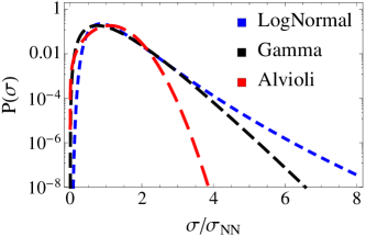
Let us consider distributional forms for along with that presented in Guzey:2005tk ; Alvioli:2013vk , we fix the mean of the proposed distributions to the average . We pick two probability distributions to model the fluctuations of the cross section: a gamma distribution and a log normal (see Fig: 1). The densities are
| (3) | ||||
| (4) | ||||
| (5) | ||||
We fix the values of and in the gamma and log-normal distributions so that both of the proposed distributions have the same variance. The Miettenen-Pumplin relation Miettinen:1978jb connects the scaled variance of to the ratio of single inelastic and elastic cross-sections at
| (6) |
Our proposed distributions have which is consistent with current experimental results.
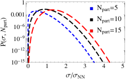
The joint probability distributions of and are shown for some fixed values of in Fig: 2. From these figures it is clear that large fluctuations in the cross section are more likely to contribute at larger values of . We compute the average cross section for each of the proposed distributions
| (7) |
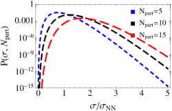
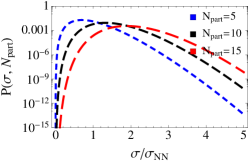
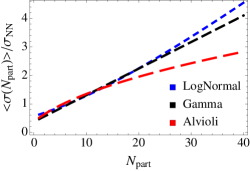
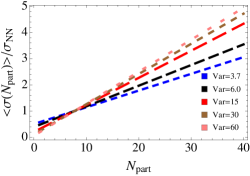
These effective cross sections are shown in Fig: 3 as a function of the number of participants. The effective cross section grows roughly linearly with the number of participants. Events with large are more likely to be events with a large cross section and thus a large effective proton area. We show the influence of the variance of the proposed cross section distributions in Fig: 4, a larger variance enhances the effective cross section for a given number of participants.
Having established that fluctuations in the cross section can be selected by requiring large fluctuations in the number of participants, let us now consider some simple models of these fluctuations.
III The Stringy Model
In the stringy model we model the fat proton as three valence quarks connected by color flux tubes. This phenomenological model is inspired by results from quenched lattice QCD which show that at even relatively modest valence quark separations the gluon field in a nucleon localizes into flux tubes Bissey:2009gw ; Bissey:2006bz . In 3-body problems it is often convenient to use Jacobi coordinates
| (8) |
In the center-of-mass (CM) frame . Neglecting spin effects, we can write a wave equation for this system as
| (9) |
where is the inter-quark potential Sakurai:1967 . Here we approximate this potential as a linear confinement potential with string constant in the limit of very spatially extended configurations. We assume a star-like configuration of flux tubes converging on the CM of the quark configuration:
| (10) |
Neglecting cross terms in the large spatial extent regime we approximate the potential for convenience as
| (11) |
The wave equation then takes the form
| (12) |
The solution for the wave function is
| (13) |
From the normalization requirement
| (14) |
we obtain . The mass of the nucleon in this simple model is
| (15) |
The mean square radius of the system is
| (16) |
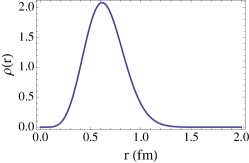
taking a string constant we obtain the root-mean-square (RMS) radius of these configurations . The fraction of configurations of radius can be computed from
| (17) |
this is plotted in Fig: 5.
.
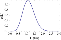
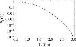
The fraction of configurations with total flux-tube length ,
| (18) |
is shown in Fig: 7. The average total flux tube length is . The probability of the total flux tube length exceeding a certain value of ,
| (19) |
is shown in Fig: 7. Configurations with very long flux tubes occur with observable frequency, for instance, we would expect there to be approximately events with with in the CMS p+Pb data.
IV The Cloudy Model
There is a non vanishing probability for a proton to produce a virtual pion via the transition or . Isospin symmetry dictates that . The proton can also produce a virtual pion and simultaneously excite itself into one of the states of the -resonance: . As this transition requires an additional 300 MeV of energy, we neglect this contribution here, but it would need to be taken into account in a more complete treatment.
Since the configuration with a single virtual pion contains either a neutron or a proton, it can spawn another virtual pion by the same mechanism. Assuming that the consecutive pion production processes are independent then the number of virtual pions accompanying the proton is given by a Poisson distribution with mean given by the average number of virtual pions . The probability of finding the incident nucleon accompanied by a cloud of pions is thus:
| (20) |
Experimental information about the virtual pion cloud of the nucleon is obtained, e. g. from exclusive pion production in electron scattering off the nucleon, or the measurement of the isovector component of the antiquark distribution in the nucleon Horn:2006tm ; DeTroconiz:2001wt ; Amendolia:1984nz . Here we focus on the second method.
IV.1 The asymmetry
Parton distribution functions (PDFs) Brock:1993sz give the unnormalized probability of finding a parton of species with a given momentum fraction in a proton at a given scale . The distributions are normalized so that
| (21) | ||||
| (22) | ||||
| (23) |
The first two integrals fix the number of valence quarks of each flavor in the proton, the third sum ensures conservation of the total momentum of the proton.
The Gottfried sum rule is given in terms of the second nucleon structure function ,
| (24) |
The naive value for this sum would be , based on the notion that sea quarks arise from the splitting of gluons, implying that the antiquark distribution functions in the nucleon are flavor symmetric. However several experiments have found a non vanishing net flavor asymmetry in the distribution of sea quarks Towell:2001nh . A review of the theory of this asymmetry can be found in Kumano:1997cy . We shall pursue the idea that the asymmetry is the consequence of the presence of a cloud of virtual pions as developed in PhysRevD.53.2586 ; PhysRevD.44.717 . The E866 results Towell:2001nh give . If we interpret the asymmetry as arising solely from the production of virtual pions we can set . Considering isospin symmetry, this leads to the conjecture .
IV.2 Antiquark distribution in the nucleon
Following PhysRevD.53.2586 ; PhysRevD.44.717 we can write down the contribution to the overall proton light antiquark PDF of a single virtual pion. This is given in terms of the convolution of the light-cone momentum distribution of a virtual pion , the probability of finding a pion with momentum fraction , and the pion antiquark PDF :
| (25) |
Where is the associated isospin Clebsch-Gordan coefficient,
| (26) |
is the nucleon-nucleon-pion form factor and is the maximum invariant momentum transferred to the pion. In the literature the following form factors are suggested Kumano:1997cy ; PhysRevD.43.3067
| (27) |
Setting , and as suggested by Kumano Kumano:1997cy we obtain the pion distribution shown in Fig: 8. Here we have chosen such that the distribution is normalized to one. This allows us to interpret as the probability for finding a pion at a given momentum fraction given that there is a pion present in the nucleon as opposed to setting the value from experimental data and interpreting it as the unconditional probability of finding a pion with momentum fraction in the nucleon. As can be seen, the choice of form factor does not have a significant influence on the pion momentum distribution. From here on we use the dipole form as it is the median curve in Fig: 8. The average pion momentum is relatively independent of the form factor
| (28) |
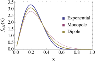
Let us consider the probability of observing a light antiquark conditioned on the number of pions present in the system. The conditional probability of observing a light antiquark given that there are no pions, , is
| (29) |
where for simplicity we are taking the nucleon PDF as being defined in the absence of virtual pions. The conditional probability for observing a light antiquark with momentum fraction given that there is a single pion accompanying the proton is
| (30) |
The probability for finding a light antiquark with momentum fraction and there being a single pion in the system is the sum of terms representing the probability of finding the light antiquark within the pion and the probability of finding the light antiquark in the proton given that the pion has taken away a fraction of the proton’s total momentum. Similarly we can write down the conditional probabilities for configurations with more virtual pions. As an example, we give the result for :
| (31) |
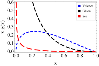
In our evaluation of these expressions we use the parameterization given by Glück et al. Gluck:1991ey for the pion PDF . For these PDFs, at GeV the average valence antiquark momentum fraction is . For reference we plot the valence, sea and gluon PDFs of the pion in Fig: 9.
| 0 | 0.889 | 2.292 |
|---|---|---|
| 1 | 0.104 | 0.747 |
| 2 | 0.00618 | 0.068 |
| 3 | 0.00024 | 0.0027 |
| 4 |
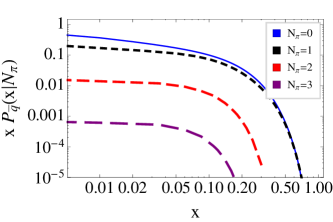
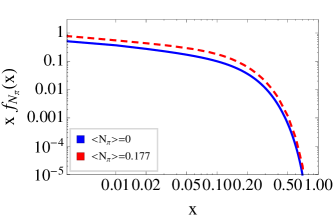
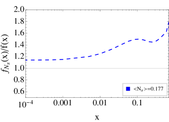
We tabulate the probabilities of finding pions in the physical proton along with the integral of the modified PDF in Table: 1. The contributions from configurations with different numbers of virtual pions to the antiquark distribution are shown in Fig: 10. The contributions die off quickly with , the higher order terms contribute to successively smaller ranges in due to the conservation of the total momentum of the proton. The modified PDF including effects from up to three pions,
| (32) |
is shown in Fig: 11.
V Phenomenology
V.1 Effects on Hard Scattering
An observable consequence of the stringy proton model would be an enhancement of gluon jet production over quark jets in high multiplicity p+Pb events. We expect that the gluon density in a “fat” nucleon will be enhanced at moderate to large , as almost all of the energy in the proton now resides in the gauge field contained in the flux-tubes. This implies that the momentum fraction carried by the valence quarks must be shifted to smaller values of . We expect that the localization of the valence quarks and the enhanced large- gluon distribution will have a non trivial feed-down to saturation physics at small . However a more detailed calculation is needed to address the small- physics associated with a high multiplicity p+Pb event. We expect that the total cross-section fluctuations arising from this model would scale like fluctuations in the total area of the nucleon, this is set by
| (33) |
where is plotted in Fig: 5.
In the case of the cloudy proton model, the presence of virtual pions in the “fat” proton serves to enhance the antiquark PDF at large values of . This enhancement must be accompanied by a shift of the light quark distribution to smaller values of . This could lead to an observable enhancement of hard quark-antiquark annihilation, expressed as enhanced Drell-Yan pair-production or as enhanced W-boson production in high multiplicity events relative to a minimum bias baseline.
We note that in both models the valence quark distribution will be shifted to lower values of , implying reduced production of very hard jets initiated by valence quark scattering. As a consequence, in the cloudy nucleon model the gluon sea, and as a secondary effect the isoscalar quark sea will be much enhanced, while in the stringy nucleon model the isovector quark sea will be enhanced with little or no increase in the gluon sea. This difference should, in principle, serve as an observable distinction between the two models. Of course, in reality, both mechanisms may contribute to the “fat” proton configurations.
To estimate the significance of these modifications we consider the cloudy nucleon model. We can compare the average momentum fraction carried by an antiquark in the modified and unmodified situations,
| (34) |
we use a lower cut-off of . In terms of the antiquark distribution inside the virtual pion we can estimate
| (35) |
using data from Fig: 8 and Fig: 9. Directly integrating the MSTW PDFs for nucleon sea antiquarks we find
| (36) |
This means that the antiquarks contributed by virtual pions carry, on average, three times the longitudinal momentum than the antiquarks contained in the parton sea of an average proton. This difference should be possible to observe if the population of protons with a virtual pion can be significantly enhanced by selecting high-multiplicity p+Pb events. The fully modified PDF (32) including the effects of up to three virtual pions gives
| (37) |
a value times larger than the unmodified case. The virtual pions make a significant contribution to the nucleon PDF. We can expect some modification to hard processes as a result.
We refrain here from making quantitative predictions for hard scattering phenomena accompanying high multiplicity p+Pb events, because these will certainly depend sensitively on the possible trigger conditions, which are not known to us. We also are concerned that the sophistication of the models of the “fat” proton explored here, especially the “stringy” proton model, is insufficient to make reliable quantitative predictions for the effective parton distributions associated with a given multiplicity window.
V.2 Eccentricity Distributions
How else can we physically distinguish between these two toy models? By considering their influence on the parton distributions we have examined the fat proton in a longitudinal section. We now attempt to build models of the transverse structure of the portly proton. We numerically sample the spatial eccentricity coefficients from density distributions generated in the spirit of each of the models. If the energy deposited in a proton-nucleus collision thermalizes and the tiny fireball expands hydrodynamically, these spatial eccentricities may reasonably be expected to be reflected in the Fourier coefficients of the final-state flow .
We compute the eccentricities for an event with a transverse density profile as
| (38) |
where the event plane angle for the th moment is
| (39) |
We generate events for the pion cloud model with pions as follows, where is drawn from the Poisson distribution (20) . For each event we sample the radial locations of the pions about the proton from an exponential distribution. The pion angular positions are sampled uniformly. The exponential radial distribution is motivated by the Yukawa model, we consider several values of the rate constant for this distribution. In PhysRevD.53.2586 the authors carry out a more advanced calculation along the same lines as our cloudy model, including the effects of the channel. The dominant contribution of the pion cloud to the antiquark distribution arises from pions with an average momentum of GeV, although this calculation is carried out at a slightly lower virtuality scale this result provides a reasonable estimate for the mean radial position of pions around the proton. We set our the average pion radial position to be .
A Gaussian kernel with width fm is convolved against the resulting points. This kernel width is chosen so that . We take the radius of the proton as defining the distance from the center, i.e the probability of finding any density outside of this radius is . Finally a density representing the proton is placed at the origin with a smearing kernel width of fm.


Density plots of a few typical events from the pion model are shown in Fig: 12, here the plots have a width of fm. The central proton tends to dominate the density but the effects of the outlying pions are visible. We consider one ensemble with the average number of pions set to the physical value of and one with to illustrate the effects of large fluctuations.
For the stringy model we sample the absolute values of the Jacobi parameters normally with some width such that the average total flux tube length is fm, to match the values we computed above. The angles made by in the transverse plane are sampled uniformly, the positions of the three quarks can then be reconstructed.


The flux tube density profile is generated by convolving the resulting line segments with a Gaussian profile. We consider two ensembles, a “thin” and “fat” set of events with widths fm respectively. Some typical events are shown in Fig: 13. These plots are fm in width, long two-legged configurations tend to dominate.
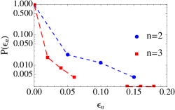
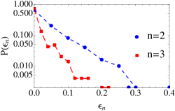
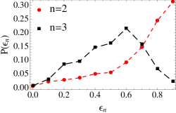
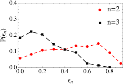
Histograms of the distributions for the pion cloud and stringy models are shown in Fig: 14 and Fig: 15. The pion model with a realistic average number of pions per nulceon gives an appreciably non-zero eccentricity distribution, this is strongly enhanced in for the large pion cloud case.
Either choice of flux tube width leads to strong enhancements in the spectrum at large eccentricities and to a nontrivial spectrum, the wider string model shows less dramatic results as the smearing reduces the geometric influence of the string profile.
VI Summary and Outlook
Fluctuations in the nucleon-nucleon cross section can induce large fluctuations in the number of participants in a central p+Pb event. The apparent universality of the large tails of p+Pb, Pb+Pb and p+p collisions suggests these fluctuations arise from a spatially over-extended, or “fat”, proton wave function. A natural consequence of this extended proton size and its concomitant large cross section is an enhanced collision volume in such p+Pb events. The larger volume reduces spatial density gradients and thus makes a hydrodynamical description of the evolution of the reaction more likely to be valid.
We have proposed two phenomenological models for the large-size configurations of the proton, one based on color flux tubes and one on virtual pion production. Each model leads to modified large physics in the initial state of the p+Pb collision relative to minimum bias events. Qualitatively, the stringy proton model predicts enhancement of the gluon PDF, while the cloudy proton model predicts an enhancement of the light antiquark PDFs. It would be interesting to view these models as different initial seeds for small saturation physics. The stringy model’s extended “valence” gluon configuration is likely to give rise to a substantially different color glass than that arising from the pion cloud which effectively has many more valence (anti-)quarks.
In proton-nucleus collisions the conjectured “fat” proton configurations have obvious consequences for the transverse energy density distribution in the initial state and its Fourier moments . The much enhanced initial transverse extent of the fireball makes the application of hydrodynamical models for its expansion more credible, because it implies a larger Knudsen number. Since the distribution of eccentricities is significantly different for the two models considered here, measurements of final-state “flow” coefficients for high multiplicity p+Pb events will shed some light upon which of these models is more realistic.
Acknowledgements.
We acknowledge support by DOE grant DE-FG02-05ER41367. CCS would like to thank D. Velicanu and I. C. Kozyrkov for many helpful discussions.References
- (1) CMS Collaboration, S. Chatrchyan et al., (2013), arXiv:1305.0609.
- (2) CMS Collaboration, S. Chatrchyan et al., Physics Letters B 718, 795 (2013).
- (3) M. Good and W. Walker, Phys.Rev. 120, 1857 (1960).
- (4) B. Kopeliovich, L. Lapidus, and A. Zamolodchikov, JETP Lett. 33, 595 (1981).
- (5) B. Blaettel, G. Baym, L. Frankfurt, H. Heiselberg, and M. Strikman, Phys.Rev. D47, 2761 (1993).
- (6) A. Bialas and A. Bzdak, Acta Phys.Polon. B38, 159 (2007), arXiv:hep-ph/0612038.
- (7) L. Frankfurt, M. Strikman, D. Treleani, and C. Weiss, Phys.Rev.Lett. 101, 202003 (2008), arXiv:0808.0182.
- (8) P. Bozek, Phys.Rev. C85, 014911 (2012), arXiv:1112.0915.
- (9) P. Bozek and W. Broniowski, Phys.Lett. B718, 1557 (2013), arXiv:1211.0845.
- (10) P. Bozek and W. Broniowski, Phys.Lett. B720, 250 (2013), arXiv:1301.3314.
- (11) P. Bozek and W. Broniowski, (2013), arXiv:1304.3044.
- (12) G.-Y. Qin and B. Müller, (2013), arXiv:1306.3439.
- (13) M. Alvioli and M. Strikman, (2013), arXiv:1301.0728.
- (14) M. Rybczynski and Z. Wlodarczyk, (2013), arXiv:1307.0636.
- (15) The Totem Collaboration, G. Antchev et al., EPL (Europhysics Letters) 101, 21003 (2013).
- (16) V. Guzey and M. Strikman, Phys.Lett. B633, 245 (2006), arXiv:hep-ph/0505088.
- (17) H. I. Miettinen and J. Pumplin, Phys.Rev. D18, 1696 (1978).
- (18) F. Bissey, A. Signal, and D. Leinweber, Phys.Rev. D80, 114506 (2009), arXiv:0910.0958.
- (19) F. Bissey et al., Phys.Rev. D76, 114512 (2007), arXiv:hep-lat/0606016.
- (20) J. Sakurai, Advanced Quantum Mechanics (Addison-Wesley, 1967).
- (21) Jefferson Lab F(pi)-2 Collaboration, T. Horn et al., Phys.Rev.Lett. 97, 192001 (2006), arXiv:nucl-ex/0607005.
- (22) J. De Troconiz and F. Yndurain, Phys.Rev. D65, 093001 (2002), arXiv:hep-ph/0106025.
- (23) S. Amendolia et al., Phys.Lett. B146, 116 (1984).
- (24) CTEQ Collaboration, R. Brock et al., Rev.Mod.Phys. 67, 157 (1995).
- (25) FNAL E866/NuSea Collaboration, R. Towell et al., Phys.Rev. D64, 052002 (2001), arXiv:hep-ex/0103030.
- (26) S. Kumano, Phys.Rept. 303, 183 (1998), arXiv:hep-ph/9702367.
- (27) W. Koepf, L. L. Frankfurt, and M. Strikman, Phys. Rev. D 53, 2586 (1996).
- (28) S. Kumano and J. T. Londergan, Phys. Rev. D 44, 717 (1991).
- (29) S. Kumano, Phys. Rev. D 43, 3067 (1991).
- (30) M. Gluck, E. Reya, and A. Vogt, Z.Phys. C53, 651 (1992).