MiRage: An Iterative MapReduce based Frequent Subgraph Mining Algorithm

Abstract

Frequent subgraph mining (FSM) is an important task for exploratory data analysis on graph data. Over the years, many algorithms have been proposed to solve this task. These algorithms assume that the data structure of the mining task is small enough to fit in the main memory of a computer. However, as the real-world graph data grows, both in size and quantity, such an assumption does not hold any longer. To overcome this, some graph database-centric methods have been proposed in recent years for solving FSM; however, a distributed solution using MapReduce paradigm has not been explored extensively. Since, MapReduce is becoming the de-facto paradigm for computation on massive data, an efficient FSM algorithm on this paradigm is of huge demand. In this work, we propose a frequent subgraph mining algorithm called MiRage which uses an iterative MapReduce based framework. MiRage is complete as it returns all the frequent subgraphs for a given user-defined support, and it is efficient as it applies all the optimizations that the latest FSM algorithms adopt. Our experiments with real life and large synthetic datasets validate the effectiveness of MiRage for mining frequent subgraphs from large graph datasets. The source code of MiRage is available from www.cs.iupui.edu/~alhasan/software/

I Introduction

In recent years, the “big data” phenomenon has engulfed a significant number of research and application domains including data mining, computational biology [1], environmental sciences, e-commerce [2], web mining, and social network analysis [3]. In these domains, analyzing and mining of massive data for extracting novel insights has become a routine task. However, traditional methods for data analysis and mining are not designed to handle massive amount of data, so in recent years many such methods are re-designed and re-implemented under a computing framework that is aware of the big-data syndrome.

Among the recent efforts for building a suitable computing platform for analyzing massive data, the MapReduce [4] framework of distributed computing has been the most successful. It adopts a data centric approach of distributed computing with the ideology of “moving computation to data”; besides it uses a distributed file system that is particularly optimized to improve the IO performance while handling massive data. Another main reason for this framework to gain attention of many admirers is the higher level of abstraction that it provides, which keeps many system level details hidden from the programmers and allows them to concentrate more on the problem specific computational logic.

MapReduce has become a popular platform for analyzing large networks in recent years. However, the majority of such analyses are limited to estimating global statistics (such as diameter) [5], spectral analysis [6], or vertex-centrality analysis [5]. Efforts for mining sub-structure is not that common, except a few works for counting triangles [7]. Specifically, frequent subgraph mining on MapReduce has received the least attention. Given the growth of applications of frequent subgraph mining in various disciplines including social networks, bioinformatics [8], cheminformatics [9], and semantic web [10], a scalable method for frequent subgraph mining on MapReduce is of high demand.

Solving the task of frequent subgraph mining (FSM) on a distributed platform like MapReduce is challenging for various reasons. First, an FSM method computes the support of a candidate subgraph pattern over the entire set of input graphs in a graph dataset. In a distributed platform, if the input graphs are partitioned over various worker nodes, the local support of a subgraph at a worker node is not much useful for deciding whether the given subgraph is frequent or not. Also, local support of a subgraph in various nodes cannot be aggregated in a global data structure, because, MapReduce programming model does not provide any built-in mechanism for communicating with a global state. Also, the support computation cannot be delayed arbitrarily, as following Apriori principle [11], future candidate frequent patterns  can be generated only from a frequent pattern.

In this paper, we propose, MiRage , a distributed frequent subgraph mining method over MapReduce. MiRage generates a complete set of frequent subgraphs for a given minimum support threshold. To ensure completeness, it constructs and retains all patterns that have a non-zero support in the map phase of the mining, and then in the reduce phase, it decides whether a pattern is frequent by aggregating its support from different computing nodes. To overcome the dependency among the states of a mining process, MiRage runs in an iterative fashion, where the output from the reducers of iteration $i-1$ is used as an input for the mappers in the iteration $i$. The mappers of iteration $i$ generate candidate subgraphs of size $i$ (number of edge), and also compute the local support of the candidate pattern. The reducers of iteration $i$ then find the true frequent subgraphs (of size $i$) by aggregating their local supports. They also write the data in disk that are processed in subsequent iterations.

We claim the following contributions:

• We introduce, MiRage, a novel iterative MapReduce based frequent subgraph mining algorithm, which is complete.

• We design novel data structures to save and consequently propagate the states of the mining process over different iterations.

• We empirically demonstrate the performance of MiRage on synthetic as well as real world large datasets.

II Related Works

There exist may algorithms for solving the in-memory version of frequent subgraph mining task, most notable among them are AGM [12], FSG [13], gSpan [14], and Gaston [15]. These methods assume that the dataset is small and the mining task finishes in a reasonable amount of time using an in-memory method. To consider the large data scenario, a few traditional database based graph mining algorithms, such as, DB-Subdue [16], and DB-FSG [17] are also proposed.

Researchers also considered shared memory parallel algorithms for frequent subgraph mining. Cook et al. presented a parallel version of their frequent subgraph mining algorithm Subdue [18]. Wang et al. developed a parallel toolkit [19] for their MotifMiner [20] algorithm. Meinl et al. created a software named Parmol [21] which includes parallel implementation of Mofa [22], gSpan [14], FFSG [23] and Gaston [15]. ParSeMis[24] is another such tool that provides parallel implementation of gSpan algorithm. To deal with the scalability problem caused by the size of input graphs, there are couple of notable works, PartMiner [25] and PartGraphMining [26], which are based on the idea of partitioning the graph data.

MapReduce framework has been used to mine frequent patterns that are simpler than a graph, such as, a set [27, 28, 29, 30], and a sequence [31]. In [32], the authors consider frequent subgraph mining on MapReduce, however, their approach is inefficient due to various shortcomings. The most notable is that in their method they do not adopt any mechanism to avoid generating duplicate patterns. This cause an exponential increase in the size of the candidate subgraph space; furthermore, the output set contains duplicate copy of the same graph patterns that are hard to unify as the user has to provide a subgraph isomorphism routine for this amendment. Another problem with the above method is that it requires the user to specify the number of MapReduce iterations. Authors did not mention how to find the total iteration count so that the algorithm is able to find all frequent patterns for a given support. One feasible way might be to set the iteration count to the edge count of the largest transaction but that will be an overkill of the resources. MiRage does not suffer from any of the above limitations.

There also exist a couple of works that mine subgraphs that are frequent considering the embedding count of that graph in a single large graph [33][34]. Wu et al. developed a distributed subgraph mining algorithm [33] which requires the graph diameter and the number of vertices for pattern matching. Liu et al. proposed an algorithm MRPF [34] that find motifs in prescription compatibility network. Fatta et al. [35] used a search tree partitioning approach, along with dynamic load balancing, for mining molecular structures.

III Background

Figure 1: (a) Graph database with 3 graphs with labeled vertices (b) Frequent subgraph of (a) with $minsup=2$

III-A Frequent Sub-graph Mining

Let, ${\cal G}=\{G_{1},G_{2},\ldots,G_{n}\}$ be a graph database, where each $G_{i}\in{\cal G},\forall i=\{1\ldots n\}$ represents a labeled, undirected and connected graph. For a graph $g$, its size is defined as the number of edges it contains. Now, t$(g)=\{G_{i}:g\subseteq G_{i}\in{\cal G}\},\forall i=\{1\ldots n\}$, is the support-set of the graph $g$ (here the subset symbol denotes a subgraph relation). Thus, t$(g)$ contains all the graphs in ${\cal G}$ that has a subgraph isomorphic to $g$. The cardinality of the support-set is called the support of $g$. $g$ is called frequent if $support\geq\pi^{\textbf{min}}$, where $\pi^{\textbf{min}}$ is predefined/user-specified minimum support (minsup) threshold. The set of frequent patterns are represented by ${\cal F}$. Based on the size (number of edges) of a frequent pattern, we can partition ${\cal F}$ into a several disjoint sets, ${\cal F}_{i}$ such that each of the ${\cal F}_{i}$ contains frequent patterns of size $i$ only.

Example: Figure 1(a) shows a database with 3 vertex labeled graphs ($G_{1}$, $G_{2}$ and $G_{3}$). With $\pi^{\textbf{min}}=2$, there are thirteen frequent subgraphs as shown in Figure 1(b). Note that, For the sack of simplicity in this example we assume that the edges of the input graphs are unlabeled. But MiRage is designed and developed to handle labels both on vertices and edges.  

III-B MapReduce

MapReduce is a programming model that enables distributed computation over massive data [4]. The model provides two abstract functions: map, and reduce. Map corresponds to the “map” function and reduce corresponds to the “fold” function in functional programming. Based on its role, a worker node in MapReduce is called a mapper or a reducer. A mapper takes a collection of (key, value) pairs and applies the map function on each of the pairs to generate an arbitrary number of (key,value) pairs as intermediate output. The reducer aggregates all the values that have the same key in a sorted list, and applies the reduce function on that list. It also writes the output to the output file. The files (input and output) of MapReduce are managed by a distributed file system. Hadoop is an open-source implementation of MapReduce programming model written in Java language.

Iterative_MapReduce(): 1.  While(Condition) 2.    Execute MapReduce Job 3.    Write result to DFS 4.    Update condition

Figure 2: Iterative MapReduce Algorithm

III-B1 Iterative MapReduce

Iterative MapReduce [36] can be defined as a multi staged execution of map and reduce function pair in a cyclic fashion, i.e. the output of the stage $i$ reducers is used as an input of the stage $i+1$ mappers. An external condition decides the termination of the job. Pseudo code for iterative MapReduce algorithm is presented in Figure 2.

IV Method

MiRage is designed as an iterative MapReduce process. At the beginning of iteration $i$, MiRage has at its disposal all the frequent patterns of size $i-1$ (${\cal F}_{i-1}$), and at the end of iteration $i$, it returns all the frequent patterns of size $i$, $({\cal F}_{i})$. Note that, in this work, the size of a graph is equal to the number of edges it contains. Now, for a mining task, if ${\cal F}$ is the set of frequent patterns MiRage runs for a total of $l$ iterations, where $l$ is equal to the size of the largest graph in ${\cal F}$.

To distribute a frequent subgraph mining (FSM) task, MiRage partitions the graph dataset ${\cal G}=\{G_{i}\}_{i=1\ldots n}$ into $k$ disjoint partitions, such that each partition contains roughly equal number of graphs; thus it mainly distributes the support counting (discussed in details later) subroutine of a frequent pattern mining algorithm. Conceptually, each node of MiRage runs an independent FSM task over a graph dataset which is $1/k$’th of the size of $|{\cal G}|$. The FSM algorithm that MiRage implements is an adaptation of the baseline algorithm shown in Figure 3, which runs in a sequential machine. Below we provides more details of this algorithm.

// ${\cal G}$ is the database // $k$ is initialize to 1 Mining_Frequent_Subgraph(${\cal G},minsup$): 0.  Populate ${\cal F}_{1}$ 1.  while ${\cal F}_{k}\neq\emptyset$ 2.    ${\cal C}_{k+1}$ = Candidate_generation(${\cal F}_{k},{\cal G}$) 2.    forall $c\in{\cal C}_{k+1}$ 3.      if isomorphism_checking($c$) = true
4.        support_counting($c,{\cal G}$)
5.        if $c.sup\geq minsup$ 6.          ${\cal F}_{k+1}$ = ${\cal F}_{k+1}\bigcup\{c\}$ 7.    $k=k+1$ 8.  return $\bigcup_{i=1\cdots k-1}{{\cal F}_{i}}$

Figure 3: Frequent subgraph mining algorithm with breadth-first candidate enumeration

IV-A Baseline frequent subgraph mining algorithm

The pseudo-code shown in Figure 3 implements an FSM algorithm that follows a typical candidate-generation-and-test paradigm with breadth-first candidate enumeration. In this paradigm, the mining task starts with frequent patterns of size one (single edge patterns), denoted as ${\cal F}_{1}$ (Line 0). Then in each of the iterations of the while loop (Line 1-6), the method progressively finds ${\cal F}_{2},{\cal F}_{3}$ and so on until the entire frequent pattern set (${\cal F}$) is obtained. If ${\cal F}_{k}$ is non-empty at the end of an iteration of the above while loop, from each of the frequent patterns in ${\cal F}_{k}$ the mining method creates possible candidate frequent patterns of size $k$+1 (Line 2). These candidate patterns are represented as the set ${\cal C}$. For each of the candidate patterns, the mining method computes the pattern’s support against the dataset ${\cal G}$ (Line 5). If the support is higher than the minimum support threshold ($minsup$), the given pattern is frequent, and is stored in the set ${\cal F}_{k+1}$ (Line 6). Before support counting, the method also ensures that different isomorphic forms of a unique candidate patterns are unified and only one such copy is processed by the algorithm (Line 4). Once all the frequent patterns of size $k+1$ are obtained, the while loop in Line 1 to 7 continues. Thus each iteration of the while loop obtains the set of frequent patterns of a fixed size, and the process continues until all the frequent patterns are obtained. In Line 8, the FSM algorithm returns the union of ${\cal F}_{i}:1\leq i\leq k-1$.

Below, we provide a short description of each of the subroutines that are called in the pseudo-code.

Figure 4: Candidate generation subtree rooted under $A-B$

IV-A1 Candidate Generation

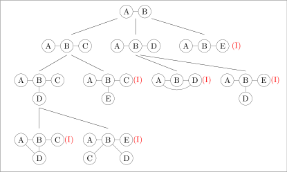
Given a frequent pattern (say, $c$) of size $k$, this step adjoins a frequent edge (which belongs to ${\cal F}_{1}$) with $c$ to obtain a candidate pattern $d$ of size $k+1$. If $d$ contains an additional vertex then the added edge is called a forward edge, otherwise it is called a back edge; the latter simply connects two of the existing vertices of $c$. Additional vertex of a forward edge is given an integer id, which is the largest integer id following the ids of the existing vertices of $c$; thus the vertex-id stands for the order in which the forward edges are adjoined while building a candidate pattern. In graph mining terminology, $c$ is called the parent of $d$, and $d$ is a child of $c$, and based on this parent-child relationship we can arrange the set of candidate patterns of a mining task in a candidate generation tree (see Figure 4). Note that, if $d$ has $k+1$ edges, based on the order how its edges has been adjoined, $d$ could have many different generation paths in a candidate generation tree; however, in all FSM algorithms, only one of the generation paths is considered valid, so that multiple copies of a candidate pattern is not generated. With this restriction of candidate generation, the candidate generation tree of an FSM task can be unambiguously defined.

Existing FSM algorithms also impose restriction on the extension nodes of the parent pattern so that redundant generation paths can be reduced. One such restriction that is used in the popular gSpan algorithm [14] is called rightmost path generation that allows adjoining edges only with vertices on the rightmost path. Simple put, “right most vertex” (RMV) is the vertex with the largest id in a candidate subgraph and “right most path” (RMP) is the shortest path from the lowest id vertex to the RMV strictly following forward edges.

Example: In Figure 4, we show a part of the candidate generation tree of the FSM task that we define in Figure 1. Suppose we have explored all frequent level-1 patterns ($g_{1}$ to $g_{4}$ in Figure 1(b)) and we want to generate candidates from one of those patterns, namely $A-B$. Figure 4 shows the part of the candidate generation subtree that is rooted at the pattern $A-B$. The nodes at the level 2 (root of the subtree is level 1) of this subtree shows all possible candidate patterns of size 2 that are built by adjoining the edge $B-C$, $B-D$, and $B-E$, respectively, with the pattern $A-B$. Note that, all these candidate patterns are created by introducing a forward edge as adding a back edge will create a multi-graph, which we do not allow. Also note, we do not extend $A-B$ with another copy of $A-B$ to create the pattern $A-B-A$ because none of the database graphs in Figure 1(a) has multiple copies of the edge $A-B$. Among these three candidate patterns, the pattern $A-B-E$ is infrequent which is denoted with the mark $(I)$ near the pattern. The remaining two patterns are frequent and are extended further to generate level-3 candidates For example, the pattern $A-B-D$ is extended with an back-edge to obtain the triangle pattern $A-B-D$ (all level-3 or level-4 nodes are not shown).  

There are other important observations in Figure 4. First, the extension of a pattern is only made on the rightmost path of that pattern. For visual clarification, for each pattern we draw its rightmost path along a horizontal line. The second observation is that, the duplicate generation paths are avoided; for example, the pattern $B-\{A,C,D\}$ (the first pattern from the left on level-3) is generated from the pattern $A-B-C$, but not from the pattern $A-B-D$,

Figure 5: Graph isomorphism

IV-A2 Isomorphism checking

As we mention in previous paragraph, a candidate pattern can be generated from multiple generation paths, but only one such path is explored during the candidate generation step and the remaining paths are identified and subsequently ignored. To identify invalid candidate generation paths, a graph mining algorithm needs to solve the graph isomorphism task, as the duplicate copies of a candidate patterns are isomorphic to each other. A well-known method for identifying graph isomorphism is to use canonical coding scheme, which serializes the edges of a graph using a prescribed order and generates a string such that all isomorphic graphs will generate the same string. There are many different canonical coding schemes, min-dfs-code is one of those which is used in [14]. According to this scheme, the generation path of a pattern in which the insertion order of the edges matches with the edge ordering in the min-dfs-code is considered as the valid generation path, and the remaining generation paths are considered as duplicate and hence ignored. MiRage uses min-dfs-code based canonical coding for isomorphism checking.

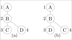
Example: Figure 5(a) and Figure 5(b) shows two isomorphic forms of the pattern $B-\{A,C,D\}$, however during candidate generation phase the first is generated from $A-B-C$ wheres the second would have been generated from $A-B-D$. According to the canonical coding scheme in [14], the pattern in Figure 5(a) is mapped to a code-string $(1,2,A,B)(2,3,B,C)(2,4,B,D)$ in which each parenthesized part is an edge written in the format $(id_{1},id_{2},label_{1},label_{2})$. Using the same coding scheme, the pattern in Figure 5(b) is mapped to the string $(1,2,A,B)(2,3,B,D)(2,4,B,C)$. However, the min-dfs-code of the pattern $B-\{A,C,D\}$ is $(1,2,A,B)(2,3,B,C)(2,4,B,D)$, which matches with the isomorphic form shown in Figure 5(a); thus the pattern will only be generated by extending $A-B-C$. Other generation paths, including the one that extends $A-B-D$ are invalid and hence are ignored after performing isomorphism checking.  

Figure 6: Support Counting

IV-A3 Support Counting

Support counting of a graph pattern $g$ is important to determine whether $g$ is frequent or not. To count $g$’s support we need to find the database graphs in which $g$ is embedded. This mechanism requires solving a subgraph isomorphism problem, which is ${\cal NP}$-complete. One possible way to compute the support of a pattern without explicitly performing the subgraph isomorphism test across all database graphs is to maintain the occurrence-list (OL) of a pattern; such a list stores the embedding of the pattern (in terms of vertex id) in each of the database graphs where the pattern exists. When a pattern is extended to obtain a child pattern in the candidate generation step, the embedding of the child pattern must include the embedding of the parent pattern, thus the occurrence-list of the child pattern can be generated efficiently from the occurrence list of its parent. Then the support of a child pattern can be obtained trivially from its occurrence-list.

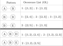
Example: In Figure 6 we illustrate a simple scenario of support counting based on occurrence list. In the top three rows of Figure 6, we show the OL of the pattern $A-B$, $B-D$ and $B-E$. The Pattern $A-B$ occurs in Graph $G_{1}$ and $G_{2}$ in vertex pair $(1,2)$ and $(1,2)$, respectively; so its OL is: 1:[(1,2)]; 2:[(1,2)]. If we adjoin $B-D$ with the pattern $A-B$ and form the pattern $A-B-D$, then we can construct the OL of $A-B-D$ (shown in 4th row) by intersecting the OLs of $A-B$ and $B-D$. Note that, the intersection considers both the graph ids and the vertex ids in the OLs. By counting the graph ids present in an OL we can compute the support of that pattern. In Figure 6, the pattern $A-B-D$ is frequent given minimum support $2$ but the pattern $A-B-E$ is not frequent.  

Mapper_FSG(${\cal F}_{k}^{p}\langle x.\textrm{min-dfs-code},x.obj\rangle$): 1.  ${\cal C}_{k+1}$ = Candidate_generation(${\cal F}_{k}^{p}$) 2.  forall $c\in{\cal C}_{k+1}$ 3.    if isomorphism_checking($c$) = true
4.      populate_occurrence_List($c$)
5.      if $length(c.occurrence\_List)>0$ 6.        emit $(c.$min-dfs-code$~{},~{}c.obj)$

Figure 7: Mapper of Distributed Frequent Subgraph Mining Algorithm

Reducer_FSG($c.$min-dfs-code$~{},\langle~{}c.obj~{}\rangle$): 1.  forall $obj\in\langle~{}c.obj~{}\rangle$ 2.    support += $length(obj.OL)$ 3.  if support $\geq$ minsup
4.    forall $obj\in\langle~{}c.obj~{}\rangle$ 5.      write $(c.$min-dfs-code$~{},~{}obj)$ to HDFS

Figure 8: Reducer of Distributed Frequent Subgraph Mining Algorithm

IV-B Distributed paradigm of MiRage

An important observation regarding the baseline FSM algorithm (Figure 3) is that it obtains all the frequent patterns of size $k$ in one iteration of while loop from Line 1 to Line 6. The tasks in such an iteration comprise to one MapReduce iteration of MiRage. Another observation is that, when the FSM algorithm generates the candidates of size $k+1$, it requires the frequent patterns of size $k$ (${\cal F}_{k}$). In an iterative MapReduce, there is no communication between subsequent iterations. So, $k+1$’th iteration of MiRage obtains ${\cal F}_{k}$ from the disk which is written by the reducers at the end of the $k$’th iteration. A final observation is that, deciding whether a given pattern is frequent or not requires counting it’s support over all the graphs in the dataset (${\cal G}$). However, as we mentioned earlier each node of MiRage works only on a disjoint partition of ${\cal G}$. So, MiRage requires to aggregate the local support from each node to perform the task in Line 5. From the above observations we identify the distribution of mining task of MiRage among the mappers and the reducers.

Figure 7 shows the pseudo-code of a mapper. The argument ${\cal F}_{k}^{p}$ represents the set of size-$k$ frequent subgraphs having non-zero support in a specific partition $p$. The mapper reads it from Hadoop Distributed File Systems (HDFS). Each pattern (say $x$) in ${\cal F}_{k}^{p}$ is read as a key-value pair. The key is the min-dfs-code of the pattern ($x$.min-dfs-code) and the value is a pattern object ($x.obj$), here “object” stands for its usual meaning from the object oriented programming. This pattern object contains all the necessary information of a pattern i.e., its support, neighborhood lists, and occurrence list. It also contains additional data structure that are used for facilitating candidate generation from this pattern. We will discuss the pattern object in details in a later section. The mapper then generates all possible candidates of size $k+1$ (Line 1) by extending each of the patterns in ${\cal F}_{k}^{p}$. For each of the generated candidates (say, $c$), the mapper performs isomorphism checking to confirm whether $c$ is generated from a valid generation path; in other words, it tests whether $c$ passes the min-dfs-code based isomorphism test (Line 3). For successful candidates, the mapper populates their occurrence list (Line 4) over the database graphs in the partition $p$. If the occurrence list of a candidate pattern is non-empty, the mapper constructs a key-value pair, such as, $(c.\textrm{min-dfs-code},c.obj)$ and emits the constructed pair for the reducers to receive (Line 6).

Figure 8 shows the pseudo code for a reducer in distributed frequent subgraph mining. The reducer receives a set of key-value pairs, where the key is the min-dfs-code of a pattern namely $c$.min-dfs-code and the value is a list of $c.obj$’s constructed from all partitions where the pattern $c$ has a non-zero support. Reducer than iterates (Line 1) over every $c.obj$ and from the length of the occurrence list of each $c.obj$ it computes the aggregated support of $c$. If the aggregated support is equal or higher than the minimum support threshold (Line 3), the reducer writes each element in the list paired with the min-dfs-code of $c$ in HDFS for the next iteration mappers.

Figure 9: Execution Flow of MiRage 

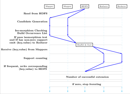
Figure 9 illustrates the execution flow of MiRage . The execution starts from the mappers as they read the key-value pair of size $k$ patterns from the HDFS. As shown in the Figure 9, the mappers generate all possible $k+1$-size candidate patterns and perform the isomorphism checking. For a pattern of size $k+1$ that passes the isomorphism test and has a non-zero occurrence, the mapper builds its key-value pair and emits that for the reducers. These key-value pairs are shuffled and sorted by the key field and each reducer receives a list of values with the same key field. The reducers then compute the support of the candidate patterns. If a pattern is frequent, the reducer writes appropriate key-value pairs in the HDFS for the mappers of the next iteration. If the number of frequent $k+1$ size pattern is zero, execution of MiRage halts.

Figure 10: (a) Framework of MiRage 

IV-C Framework of MiRage 

MiRage has three important phases: data partition, preparation phase and mining phase. In data partition phase MiRage creates the partitions of input data along with the omission of infrequent edges from the input graphs. Preparation and mining phase performs the actual mining task. Figure 10 shows a flow diagram of different phases for a frequent subgraph mining task using MiRage.

Below, we present an in-depth discussion of each of the phases.

Figure 11: Input data after partition and filtering phase

IV-C1 Data partition

In data partition phase, MiRage splits the input graph dataset ($\cal G$) into many partitions. One straightforward partition scheme is to distribute the graphs so that each partition contains the same number of graphs from ${\cal G}$. This works well for most of the datasets. However, for datasets where the size (edge count) of the graphs in a dataset vary substantially, MiRage offers another splitting option in which the total number of edges aggregated over the graphs in a partition, are close to each other. In experiment section, we show that the latter partition scheme has a better runtime performance as it improves the load balancing factor of a MapReduce job. For MiRage, the number of partition is also an important tuning parameter. In experiment section, we also show that for achieving optimal performance, the number of partitions for MiRage should be substantially larger than the number of partition in a typical MapReduce task.

During the partition phase, input dataset also goes through a filtering procedure that removes the infrequent edges from all the input graphs. While reading the graph database for partitioning, MiRage computes the support-list of each of the edges from which it identifies the edges that are infrequent for the given minimum support threshold.

Example: For the graph dataset in Figure 1, for a minimum support threshold of 2, the edges $A-B,B-C,B-D$, $D-E$ and $B-E$ are frequent and the remaining edges are infrequent. Now suppose MiRage makes two partitions for this dataset such that the first partition contains $G_{1}$, and the second partition contains $G_{2}$ and $G_{3}$. While making these partitions MiRage filters the infrequent edges. Figure 11 shows the partitioning where the infrequent edges are stripped off from the database graphs.  

Figure 12: The static data structures and $A-B-C$ pattern object in partition 1 and 2 (a) Edge-extension Map (b) Edge-OL (c) and (d) $A-B-C$ Pattern object

IV-C2 Preparation Phase

The mappers in this phase prepare some partition specific data structures such that for each partition there is a distinct copy of these data structures. They are static for a partition in the sense that they are same for all patterns generated from a partition. The first of such data structure is called edge-extension-map, which is used for any candidate generation that happens over the entire mining session. It stores the possible extension from a vertex considering the edges that exists in the graphs of a partition. For example, the graphs in partition two have edges such as $B-D,B-C,B-A$, and $B-E$. So, while generating candidates, if $B$ is an extension stub, the vertex $A,C,D$ or $E$ can be the possible vertex label of the vertex that is at the opposite end of an adjoined edge. This information is stored in the Edge-extension-map data structure for each of the vertex label that exist in a partition. The second data structure is called edge-OL, it stores the occurrence list of each of the edges that exist in a partition; MiRage use it for counting the support of a candidate pattern which is done by intersecting the OL of a parent pattern with the OL of an adjoint edge.

Example: Figure 12 (a) and Figure 12 (b) shows these data structures for the Partition 1 and 2 defined in Figure 11. In partition 1, the edge-extension choice from a vertex with label $D$ is only $B$ (shown as $D:(B)$), as in this partition $B-D$ is the only frequent edge with a $B$ vertex. On the other hand, the corresponding choice for partition 2 is $B$ and $E$ (shown as, $D:(B;E)$), because in partition 2 we have two edges, namely $B-D$ and $D-E$ that involve the $D$ vertex. In partition 1, the edge $B-D$ occurs in $G_{1}$ at vertex id $(2,4)$; on the other hand in partition 2, the same edge occurs in $G_{2}$ and $G_{3}$ at vertex id $(2,3)$ and $(1,2)$, respectively. These information are encoded in the edge-OL data structures of these partitions as shown in this figure.  

The mappers in the preparation phase also starts the mining task by emitting the frequent single edge pattern as key-value pair. Note that, since the partition phase have filtered out all the infrequent edges, all single edges that exist in any graph of any partition is frequent. As we mentioned earlier the key of a pattern is its min-dfs-code and the value is the pattern object. Each pattern object have four essential attributes: (a) Occurrence List (OL) that stores the embedding of the pattern in each graph in the partition, (b) Right-Most-Path (c) VSET that stores the embedding of the Right Most Path in each graph in the partition, and (d) support value. Mappers in the preparation phase computes the min-dfs-code and creates the pattern object for each single-edge patterns.

While emitting the key-value pair to a reducer, the mappers also bundle the static data structures, edge-extension-map and edge-OL with each of the pattern object. This is an wasteful overhead in terms of network traffic and disk space, as the static data structure is common for all the patterns that are ever generated from a partition. We had to adopt this strategy, because to the best of our knowledge there is no provision in Hadoop to keep a global data structure that can be accessed by each of the mappers. MiRage uses Java serialization to convert these objects in to byte stream while sending them as value in a key-value pair.

The reducers of this phase actually do nothing but writing the input key-value pairs in HDFS since all the single length patterns that the mappers send are frequent. In Figure 10, the second block portrays the preparation phase.

Example: Figure 12(c) and  12(d) exhibits the Pattern object along with their attributes for the pattern $A-B-C$ in partition 1 and 2, respectively. The attribute OL records the occurrence of this pattern in the corresponding database graphs; if a pattern has multiple embeddings in a database graph all such embeddings are stored. Right-Most-Path records the id of the right-most-path vertices in the pattern object and VSET stores the corresponding ids in the database graphs. Like OL, VSET is also a set and it stores information for multiple embedding if it applies. Finally, Support stores the support value of the pattern. In the following discussion, we use $\clubsuit$ and $\spadesuit$ to denote a pattern object from partition 1 ($G_{1}$) and 2 ($G_{2},G_{3}$), respectively. For example, $\spadesuit_{abc}$ identifies the pattern $A-B-C$ from partition 2 as shown in Figure 12(d).  

Figure 13: One iteration of the mining phase of MiRage with respect to pattern A-B

IV-C3 Mining Phase

In this phase, mining process discovers all possible frequent subgraphs through iteration. Preparation phase populates all frequent subgraphs of size one and writes it in the distributed file system. Iterative job starts by reading these from HDFS. Each of the mappers of an ongoing iteration is responsible for performing the mining task over a particular chunk of the data written in HDFS by the preparation phase. The map function of mining phase reconstructs all the static data structures that are required to generate candidate patterns from the current pattern. Using the static data structures and the pattern object, the mappers can independently execute the subroutine that is shown in Figure 7. The reducers in this phase simply execute the routine in Figure 8.

Example: Figure 13 provides a detail walk-through of a MapReduce job in iteration phase with respect to the partitioned toy dataset mentioned in Figure 11. Figure 13(a) and (b) indicates the key-value pairs for pattern $A-B$ from partition $1$ and $2$. Suppose these key-value pairs are feed as input for Mapper 1 and Mapper 2 in Figure 13. The mappers first extract all data structures from the value field of key-value pair including the partition-specific static data structures such as edge-extension-map and edge-OL. Then they perform the steps mentioned in Figure 7. Figure 13(c) and (d) show the key-value pairs of $A-B-C$ that are generated by Mapper 1 and Mapper 2 by extending the pattern $A-B$. The Reducer collects all the values for a key and computes the support of the pattern of of the given key by adding the supports from individual partitions. In this example, the support of the pattern $A-B-C$ is $2$; since $minsup$=2, this pattern is frequent. Reducer then writes the key-value pairs corresponding to the pattern $A-B-C$ in HDFS.  

IV-D Pseudo Code

In this section, we present the pseudo code of each phase using the syntax of Hadoop framework. Figure 14, 15 and 16 demonstrate data partitioning, preparation and mining phase, respectively. In Line 3 and 4 of Figure 14, MiRage performs the filtering and partitioning of the input dataset and writes each partition and write in the HDFS. In line 1-7 of Figure 15 the mappers generates static data structure along with emit key-value pair of all single length pattern to reducer. Since all patterns are frequent, Reducers just relay the input key,value pair to the output file in HDFS. In Line 1-3 of Mapper_mining function in Figure 16, the mappers reconstruct the pattern object of size $k$ along with the static data structures and generates the candidates from the current pattern. In Line 4-9, the mappers iterate over all possible candidates of size $k+1$ and on success in isomorphism and occurrence list test mappers emits the key-value pair for the reducer Reducer_mining function computes the aggregate support (Line 2) of the pattern and if the pattern is frequent, they write back the key,value pairs to HDFS for the mappers of the next iteration.

Partition_data(${\cal D}$): 1.  create a data directory in distributed file system 2.  while data available in ${\cal D}$ 3.    $partition$ = create_partition()
4.    write $partition$ to file $partition_{i}$ in data directory

Figure 14: Data Partitioning Phase

// key    = offset // value  = location of partition file in data directory Mapper_preparation(Long $key$, Text $value$): 1.  Generate_Level_one_OL($value$)
2.  Generate_Level_one_MAP($value$)
3.  $P$ = get_single_length_patterns()
4.  forall $P_{i}$ in $P$: 5.    $intermediate\_key$ = min-dfs-code($P_{i}$)
6.    $intermediate\_value$ = serialize($P_{i}$)
7.    emit($intermediate\_key$,$intermediate\_value$)
// key     = min-dfs-code // values  = List of Byte-stream of a pattern object in all partitions Reducer_preparation(Text $key$, BytesWritable $\langle$ values $\rangle$): 1.    for all $value$ in $values$:
2.      write_to_file($key$,$value$)

Figure 15: Preparation Phase

// key    = min-dfs-code // value  = Byte-stream of pattern object for iteration i-1 Mapper_mining(Long $key$, BytesWritable $value$): 1.  $p$ = reconstruct_pattern($value$)
2.  reconstruct_all_data-structures($value$)
3.  $P$ = Candidate_generation($p$)
4.  forall $P_{i}$ in $P$: 5.    if pass_isomorphism_test($P_{i}$) = true
6.      if $length(P_{i}.OL)>0$
7.        $intermediate\_key$ = min-dfs-code($P_{i}$)
8.        $intermediate\_value$ = serialize($P_{i}$)
9.        emit($intermediate\_key$,$intermediate\_value$)
// key     = min-dfs-code // values  = List of Byte-stream of a pattern object in all partitions Reducer_mining(Text $key$, BytesWritable $\langle values\rangle$): 1.  for all $value$ in $values$: 2.    $support$ += get_support($value$)
3.  if $support~{}\geq~{}minimum\_support$ 4.    for all $value$ in $values$: 5.      write_to_file($key,value$)

Figure 16: Mining Phase

IV-E Implementation Detail

In this section, we explain some of the implementation details of MiRage. We use Hadoop 1.1.2 a open source implementation of MapReduce framework written in Java. We use Java to write the baseline mining algorithm as well as the map and the reduce function in the preparation and the mining phase. We override the default input reader and write a custom input reader for the preparation phase. To improve the execution time of MapReduce job, we compress the data while writing them in HDFS. We used global counter provided by Hadoop to track the stopping point of the iterative mining task.

IV-E1 MapReduce Job Configuration

In this section, we provide a detail snapshot of the Map-Reduce job configuration for MiRage in Hadoop. Success of a job depends on the accurate configuration of that job. Since the type of the value that is read by a mapper and emit by a reducer is BytesWritable, MiRage sets input and output format of each job as SequenceFileInputFormat and SequenceFileOutputFormat. Another job property, named mapred.task.timeout also need to be set properly for better execution of MiRage. This parameter controls for how long the master node waits for a data node to reply. If the mining task that MiRage commence is computationally demanding, the default timeout which is 10 minutes may not be enough. To be on the safe side, MiRage sets the timeout of a job to 5 hour (300 minutes). MiRage also sets the mapred.output.compress property to true. This configuration lets the output of a MapReduce job to be compressed which eventually decreases network load and improves the overall execution time. The codec that is used for compression is BZip2Codec. MiRage also increases the heap size of a job using mapred.child.java.opts property. The same configuration is used for both the preparation and mining phase of MiRage.

V Experiments and Results

In this section, we present experimental results that demonstrate the performance of MiRage for solving frequent subgraph mining task on large graph datasets. As input, we use five real-world graph datasets which are taken from an online source  that contains graphs extracted from the PubChem website . PubChem provides information on biological activities of small molecules and the graph datasets from PubChem represent atomic structure of different molecules. In Table I, we provide the name and statistics of these datasets. We also create four synthetic datasets using a tool called Graphgen [37]. The number of graphs in these datasets range from 100K to 1000K and each graph contains on average $25-30$ edges. We conduct all experiments in a 10-node Hadoop cluster, where one of the node is set to be a master node and the remaining 9 nodes are set to serve as data node. Each machine possesses a 3.1 GHz quad core Intel processor with 16GB memory and 1 TB of storage.

Transaction	# of Transactions	Average Size of
Graph dataset		each transactions
NCI-H23	40,353	28.6
OVCAR-8	40,516	28.1
SN12C	40,532	27.7
P388	41,472	23.3
Yeast	79,601	22.8

TABLE I: Real life biological Datasets

V-A Runtime of MiRage for different minimum support

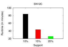
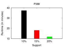
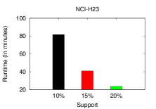
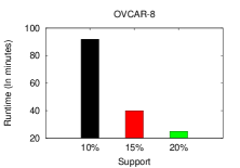
In this experiment, we analyze the runtime of MiRage for varying minimum support threshold. We conduct this experiment for biological datasets mention above. Here we fix the number of data nodes to $9$ and keep track of the running time of MiRage for minimum support thresholds that vary between $10\%$ to $20\%$. In Figure 17(a-e) we show the result. As expected, the runtime decreases with the increase of minimum support threshold.

Number of transaction	(runtime in minute)
100K	27.4
250K	69.1
750K	86.1
1000K	98.7

TABLE II: Runtime of MiRage on synthetic transaction graph datasets

V-B Runtime of MiRage for different number of database graphs

For this experiment, we generate 4 synthetic datasets each having 100K to 1000K input graphs. Each of these graphs has 25 vertices and their edge density is around $0.5$ or smaller. Table II shows the runtime of MiRage over these datasets for $30\%$ minimum support threshold using $1000$ partitions for each datasets..

(a)

(b)

(c)

(d)

(e)

Figure 17: Bar plot showing the relationship between the minimum support threshold ($\%$) and the running time (in minutes) of MiRage in (a) Yeast (b) NCI-H23 (c) P388 (d) SN12C and (e) OVCAR-8.

V-C Runtime of MiRage on varying number of data nodes

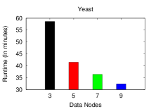
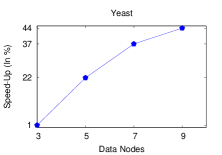
In this experiment, we demonstrate how MiRage’s runtime varies with the number of active data nodes (slaves). We use the Yeast dataset using 20% minimum support threshold. We vary the count of data nodes among 3, 5, 7 and 9 and record the execution time for each of the configurations. As shown in Figure 18(a) the runtime reduces significantly with an increasing number of data nodes. In Figure 18(b) we plot the speedup that MiRage achieves with an increasing number of data nodes, with respect to the 3-data-nodes configuration. We can see that the speedup increases almost linearly except for the last data point.

(a)

(b)

Figure 18: Relationship between the execution time and the number of data nodes: (a) Bar plot shows the execution time; (b) Line plot shows the speedup with respect to the execution time using 3 data nodes configuration

V-D Runtime of MiRage for varying number of Reducer

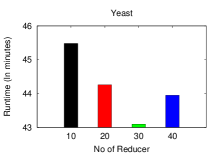
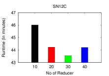
The number of reducers plays an important role in the execution of MapReduce job in Hadoop. While writing data (output) in HDFS, a MapReduce job follows a convention of naming the output file with the key word “part”. Reducer count determines how many “part” files will be generated to hold the output of a job. If the number of reducer is set to 1, entire output will be written in a single file. Since MiRage is an iterative algorithm, where output of the current job is used as an input of the next job, the number of reducer has a significant effect on the execution time of MiRage . If we set reducer count to a small value then there will be fewer number of output files that are large in size; these large files will be a burden over the network when they are transfered between data nodes. On the other hand, large number of reducers might create many output files of zero size (reducer is unable to output any frequent pattern for the next stage Mapper). These zero size output files will also become an overhead for the next stage mappers as these files will still be used as input to a mapper. Note that, loading an input file is costly in Hadoop.

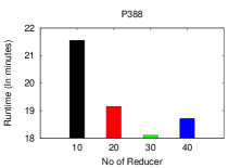
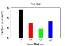
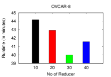
In this experiment, We measure the runtime of MiRage for various configurations such as, 10, 20, 30 and 40 reducers. We run the experiment on all 5 real-life datasets for 20% minimum support threshold. Figure 19(a-e) shows the relationship between execution time and the number of reducers using bar charts. As we can see from all the charts, 30 is the best choice for the number of reducers in our cluster setup. This finding is actually intuitive, because we have 9 data nodes each having 4 reduce slots (4 core processor), yielding 36 processing units. So keeping a few units for system use, 30 is the best choice for the number of reducers.

(a)

(b)

(c)

(d)

(e)

Figure 19: Bar plot showing the relationship between the number of Reducer and the running time of MiRage in (a) Yeast, (b) NCI-H23, (c) P388, (d) SN12C, and (e) OVCAR-8.

(a)

Figure 20: Bar plot showing the relationship between the partition count and the running time of MiRage for Yeast dataset.

V-E Runtime of MiRage for different partition sizes

An important requirement for achieving the optimal performance of a Hadoop cluster is to find the appropriate number of mappers. In such a cluster, the setup and scheduling of a task wastes a few seconds. If each of the tasks is small and the number of tasks is large, significant amount of time is wasted for task scheduling and setup. So the experts advise that a mapper should execute for at least 40 seconds . Another rule of thumbs is that the number of partition should not over-run the number of mappers.

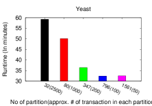
In our cluster setup, we have 9 data nodes, each with 4 cores that allow us to have 36 mappers. Then, the perfect number of input partitions should be less than or equal to $36$. But this rules does not fit well for frequent subgraph mining task. For example, the Yeast dataset has close to $80,000$ graphs and if we make $30$ partitions, then each partition ends up consisting of $2666$ graphs. Since, frequent subgraph mining is an exponential algorithm over its input size, performing a mining task over these many graphs generally becomes computationally heavy. In this case, the map function ends up taking time much more than expected. As a result the optimal number of partitions for an FSM task should set at a much higher value (compared to a tradition data analysis task) so that the runtime complexity of the mappers reduces significantly. Note that, the higher number of partitions also increases the number of key-value pairs for a given patterns which should be processed by the reducers. However, the performance gain from running FSM over small number of graphs supersedes the performance loss due to the increased number of key-value pairs. This is so, because the gain in execution time in the mappers follows an exponential function, whereas the loss in execution time in the reducers and the data transmission over the network follow a linear function.

The following experiment validates the argument that we have made in the above paragraph. In this experiment, we run MiRage on Yeast dataset for different number of partitions and compare their execution time. Figure 20 shows the result using bar charts. The charts show that as we increase the partition count, the performance keeps improving significantly until it levels off at around 1000 partitions. When the partition count is 1561, there is a slight loss in MiRage’s performance compared to the scenario when the partition count is 796. The strategy of finding the optimal number of partitions depends on the characteristics of input graphs that control the complexity of the mining task, such as the density, number of edges, number of unique labels for vertices and edges in an input graph and so on.

V-F Comparison of MiRage with an existing algorithm

As discussed in section II, [32] proposed a MapReduce based graph mining method which is inefficient due to its poor design choices. In this experiment, we compare the execution time of MiRage with that of Hill et al.’s [32] implementation that we obtain from the authors. We run both the algorithms on three real world biological dataset for $40\%$ minimum support. Table III compares the execution time between the two algorithms. As we can see MiRage performs significantly better that the other algorithm.

Dataset	MiRage (min)	Hill et. al’s[32](min)
Yeast	16.6	109.2
P388	8.3	57.5
NCI-H23	17.5	117.2

TABLE III: Runtime (in minutes) comparison between MiRage and Hill et. al’s[32] on three biological graph datasets

V-G Effect of partition scheme on runtime

In this experiment, we analyze how the partition heuristics discussed in Section IV-C1 affects the execution time of MiRage. For all datasets, We fixed minimum support to $20\%$, number of data nodes to $9$ and the number of reducer to 30. The result is shown in Table IV. We find that for schema 2, which balances the total number of edges in each partition, performs somewhat better than schema 1, which only balances the number of graphs. Note that, in the real-life graph datasets most of the graphs have similar number of edges, so the partitions using schema 1 and schema 2 have similar balance factors. But, for datasets where the input graphs have highly different number of vertices and edges, the schema 2 is obviously a better choice. To investigate further, we build a synthetic dataset of $50K$ graphs where average length of half of the graphs is around $15$ and for the other half it is around $30$. We found that for this unbalanced dataset, scheme 1 takes about 30% more time than the schema 2 (see the last row of the Table IV).

Transaction	Scheme 1	Scheme 2
Graph dataset	(runtime in min)	(runtime in min)
Yeast	32.5	30.3
SN12C	25.8	23.7
P388	11.7	10.2
NCI-H23	23.5	22
OVCAR-8	24.9	23.4
Synthetic	22.9	17.1

TABLE IV: Runtime of MiRage on different partition schemes

VI Conclusions

In this paper we present a novel iterative MapReduce based frequent subgraph mining algorithm, called MiRage. We show the performance of MiRage over real life and large synthetic datasets for various system and input configurations. We also compare the execution time of MiRage with an existing method, which shows that MiRage is significantly better than the existing method.

References

- [1] A. Rosenthal, P. Mork, M. H. Li, J. Stanford, D. Koester, and P. Reynolds, “Cloud computing: A new business paradigm for biomedical information sharing,” Journal of Biomedical Informatics, 2010.
- [2] W. Lam, L. Liu, S. Prasad, A. Rajaraman, Z. Vacheri, and A. Doan, “Muppet: Mapreduce-style processing of fast data,” Proc. VLDB Endow., 2012.
- [3] G. Liu, M. Zhang, and F. Yan, “Large-scale social network analysis based on mapreduce,” in Intl. Conference on Computational Aspects of Social Networks (CASoN), 2010.
- [4] J. Dean and S. Ghemawat, “Mapreduce: simplified data processing on large clusters,” Commun. ACM, 2008.
- [5] U. Kang, C. E. Tsourakakis, and C. Faloutsos, “Pegasus: A peta-scale graph mining system implementation and observations,” in Proceedings of the 2009 Ninth IEEE International Conference on Data Mining, 2009.
- [6] U. Kang, B. Meeder, and C. Faloutsos, “Spectral analysis for billion-scale graphs: discoveries and implementation,” in Proceedings of the 15th Pacific-Asia conference on Advances in knowledge discovery and data mining - Volume Part II, ser. PAKDD’11, 2011, pp. 13–25.
- [7] S. Suri and S. Vassilvitskii, “Counting triangles and the curse of the last reducer,” in Proceedings of the 20th international conference on World wide web, 2011.
- [8] J. Huan, W. Wang, D. B, J. Snoeyink, and J. Prins, “Mining protein family specific residue packing patterns from protein structure graphs,” in In Proc.of RECOMB, 2004.
- [9] S. Kramer, L. Raedt, and C. Helma, “Molecular feature mining in hiv data,” in In Proc.of SIGKDD, 2004, p. 136–143.
- [10] B. Berendt, “Using and learning semantics in frequent subgraph mining,” in Adv. in Web Mining and Web Usage Analysis, 2006.
- [11] R. Agrawal and R. Srikant, “Fast algorithms for mining association rules in large databases,” in Proc. of the 20th International Conference on VLDB.
- [12] A. Inokuchi, T. Washio, and H. Motoda, “An apriori-based algorithm for mining frequent substructures from graph data,” in Proc. of the 4th European Conference on Principles of Data Mining and Knowledge Discovery, ser. PKDD ’00, 2000.
- [13] M. Kuramochi and G. Karypis, “Frequent subgraph discovery,” in Proc. of Intl. Conference on Data Mining, 2001.
- [14] X. Yan and J. Han, “gSpan: Graph-based substructure pattern mining,” in Proc. of Intl. Conference on Data Mining, 2002.
- [15] S. Nijssen and J. Kok, “A quickstart in frequent structure mining can make a difference,” in Proc. of ACM SIGKDD, 2004.
- [16] S. Chakravarthy, R. Beera, and R. Balachandran, “Db-subdue: Database approach to graph mining,” in Advances in Knowledge Discovery and Data Mining, 2004.
- [17] S. Chakravarthy and S. Pradhan, “Db-fsg: An sql-based approach for frequent subgraph mining,” in Proceedings of the 19th international conference on Database and Expert Systems Applications, ser. DEXA ’08.
- [18] D. J. Cook, L. B. Holder, G. Galal, and R. Maglothin, “Approaches to parallel graph-based knowledge discovery,” Journal of Parallel and Distributed Computing, vol. 61, 2001.
- [19] C. Wang and S. Parthasarathy, “Parallel algorithms for mining frequent structural motifs in scientific data,” in Proc. of the 18th annual intl. conference on Supercomputing, 2004.
- [20] S. Parthasarathy and M. Coatney, “Efficient discovery of common substructures in macromolecules,” in In Proc. of IEEE International Conference on Data Mining, 2002.
- [21] T. Meinl, M. Worlein, O. Urzova, I. Fischer, and M. Philippsen, “The parmol package for frequent subgraph mining.” ECEASST, 2006.
- [22] C. Borgelt and M. Berthold, “Mining molecular fragments: finding relevant substructures of molecules,” in Proc.of IEEE International Conference on Data Mining, 2002.
- [23] J. Huan, W. Wang, and J. Prins, “Efficient mining of frequent subgraphs in the presence of isomorphism,” in ICDM, 2003.
- [24] M. Philippsen, M. Worlein, A. Dreweke, and T. Werth, “Parsemis - the parallel and sequential mining suite,” 2011. [Online]. Available: https://www2.cs.fau.de/EN/research/ParSeMiS/index.html
- [25] J. Wang, W. Hsu, M. L. Lee, and C. Sheng, “A partition-based approach to graph mining,” in Proc. of the 22nd International Conference on Data Engineering, 2006.
- [26] S. N. Nguyen, M. E. Orlowska, and X. Li, “Graph mining based on a data partitioning approach,” in Nineteenth Australasian Database Conference (ADC 2008), 2008.
- [27] G.-P. Chen, Y.-B. Yang, and Y. Zhang, “Mapreduce-based balanced mining for closed frequent itemset,” in IEEE 19th International Conference on Web Service, 2012, pp. 652–653.
- [28] S.-Q. Wang, Y.-B. Yang, Y. Gao, G.-P. Chen, and Y. Zhang, “Mapreduce-based closed frequent itemset mining with efficient redundancy filtering,” 2012 IEEE 12th International Conference on Data Mining Workshops, vol. 0, 2012.
- [29] L. Zhou, Z. Zhong, J. Chang, J. Li, J. Huang, and S. Feng, “Balanced parallel fp-growth with mapreduce,” in Information Computing and Telecommunications (YC-ICT), 2010 IEEE Youth Conference on, 2010.
- [30] H. Li, Y. Wang, D. Zhang, M. Zhang, and E. Y. Chang, “Pfp: parallel fp-growth for query recommendation,” in Proceedings of the 2008 ACM conference on Recommender systems, 2008.
- [31] B.-S. Jeong, H.-J. Choi, M. A. Hossain, M. M. Rashid, and M. R. Karim, “A MapReduce Framework for Mining Maximal Contiguous Frequent Patterns in Large DNA Sequence Datasets,” IETE Tech. Review, vol. 29, pp. 162–168, 2012.
- [32] S. Hill, B. Srichandan, and R. Sunderraman, “An iterative mapreduce approach to frequent subgraph mining in biological datasets,” in Proc. of the ACM Conference on Bioinformatics, Computational Biology and Biomedicine, 2012.
- [33] B. Wu and Y. Bai, “An efficient distributed subgraph mining algorithm in extreme large graphs,” in Proceedings of the 2010 international conference on Artificial intelligence and computational intelligence: Part I, 2010.
- [34] Y. Liu, X. Jiang, H. Chen, J. Ma, and X. Zhang, “Mapreduce-based pattern finding algorithm applied in motif detection for prescription compatibility network,” in Proc. of the 8th Intl. Symp. on Advanced Parallel Processing Technologies, 2009.
- [35] G. Di Fatta and M. Berthold, “Dynamic load balancing for the distributed mining of molecular structures,” Parallel and Distributed Systems, IEEE Transactions on, 2006.
- [36] J. Lin and C. Dyer, Data-Intensive Text Processing with MapReduce, 2010.
- [37] J. Cheng, Y. Ke, W. Ng, and A. Lu, “Fg-index: towards verification-free query processing on graph databases,” in SIGMOD, 2007, pp. 857–872.