Kondo effect of cobalt adatom on zigzag graphene nanoribbon

Abstract

Based on ab-initio calculations we discuss Kondo effect due to Co adatom on graphene zigzag nanoribbon. Co atom located at hollow site behaves as spin ${\cal{S}}=1/2$ impurity with $d_{xz}$ and $d_{yz}$ orbitals contributing to magnetic moment. Dynamical correlations are analyzed with the use of complementary approximations: mean field slave boson approach, noncrossing approximation and equation of motion method. The impact of interplay between spin and orbital degrees of freedom together with the effect of peculiarities of electronic and magnetic structure of nanoribbon on many-body resonances is examined.

I INTRODUCTION

Graphene possesses spectacular electronic, optical, magnetic, thermal and mechanical properties, which make it an exciting material for technological applications Novoselov ; Geim ; Castro Neto ; Das Sarma ; Katsnelson . Graphene is a semimetal. For the use in logic devices a controllable band gap is very much desired. Presence of a gap would increase tremendously the on-off ratio for current flow that is needed for many electronic applications. For example, lack of the gap prevents the use of graphene in making transistors. Band gap opening is caused by symmetry breaking Avouris ; Zhou . The most effective way within the realm of single-layer graphene physics is electron confinement e.g. in nanoribbons (partial breaking of translational symmetry) Wakabayashi ; Palacios ; Pisani ; Yang . The graphene nanoribbons (GNR) with varying widths can be realized either by cutting Hiura , mechanically exfoliated graphenes Novoselov1 or by pattering epitaxially grown graphenes Zhang . The edge geometry is the key factor which determines the electronic properties of nanoribbon. There are two types of nanoribbons, based on their edges shapes, called zigzag (ZGNR) and armchair (AGNR) Palacios ; Nakada . Recently, electronic devices, such as field effect transistors, have been formed from graphene nanoribbons Ozyilmaz ; Han . ZGNRs are of particular interest, because due to topological reasons they are forming edge states Fujita i.e. states decaying exponentially into the centre of the ribbon Castro Neto ; Brey . The decay lengths are in the range of a few nanometer Niimi . The edge states has been observed in scanning tunneling microscopy Kobayashi . The localized nature of these states gives rise to a flat band extending over one-third of the one-dimensional Brillouin zone and correspondingly also to a sharp peak in the density of states right at the Fermi level. As a consequence magnetic ground state emerges from a Fermi instability Son ; Wu . Recently the spin splitting of the edge density of states of ZGNRs has been confirmed experimentally Tao . Theoretical studies have shown that the spins on each edge are ferromagnetically ordered, and those between the edges are antiferromagnetically coupled, the later resulting from the interaction of the tails of the edge states Son2 ; Wu ; Kunstmann ; Kan1 ; Pisani . Modification of the electronic structure can be also introduced by chemical functionalization, what allows the band gap engineering and designing different types of magnetic order. Based on density functional calculations Son et al. Son have shown that one can modify the band gap of ZGNR by applying transverse electric field and that the electric field closes the gap for one of the directions selectively (half metallicity). This conclusion has been confirmed by calculations of Kan et al. Kan1 with the use of hybrid functional potential (B3LYP), which is viewed as one of the most accurate methods for estimation of the gap. The predicted critical fields of transition into half metallicity are much higer in this method than those from normal DFT calculations. It is well known, that graphene nanostructures are promising for spintronics due to their long spin relaxation and decoherence times owing to the low intrinsic spin-orbit interaction Tombros . The mentioned possibility of band gap tuning and controlling magnetism and spin transport of the ribbons by electric field is the principal advantage of these systems. The pure nanoribbon has no net magnetic moment. The functionalities of the ribbons can be enriched by doping the magnetic adatoms. Due to the open surface controlled adatoms manipulation is within reach of atomic force microscopy in these systems Seo ; Gross . In the last few years several studies focused on understanding structural, electronic and magnetic properties of $3d$ impurities in graphene nanoribbons Kan3 ; Longo ; Power ; Sevincli ; Rigo ; Cocchi . Also vacancies and defects have been predicted to give rise to magnetic moments Lehtinen ; Palacios2 . The relative stability of local moments depends on the balance between the Coulomb repulsion, exchange interaction, position of $3d$ levels and hybridization with the neighboring carbon atoms. Especially two latter factors are strongly affected by impurity location, one expects different energetics, structural, and electronic properties nearly the edge sites of GNRs and different when adatom is located inside the ribbon. The electronic structure of nanometer-wide ribbon is dominated by confinement effects and Van Hove singularities and this strongly affects the hybridization path. As opposed to normal metals, the damping of the local levels is energy dependent and the hybridization self energy acquires also significant real contribution near singularities causing effective shift of local energy levels. Since the chemical potential of GNRs can be tuned, a formation of local moment can be controlled by gate voltage and particularly strong gate dependence is expected near singularities. At low temperature, the localized spin is screened by conduction electrons and a narrow Kondo peak appears near the Fermi level. Most of the early studies in Kondo effect were carried on for the metallic systems with constant density of states at the Fermi surface, in the case of graphene structures the details of the band structure play the decisive role in screening. Recently Kondo effect has been observed in graphene both in resistivity measurements Chen and by scanning tunneling microscopy (STM) Mattos . As opposed to transport measurements STM probes local electronic properties of Kondo impurities. The Kondo resonce observed in tunneling spectroscopy usually does not show up as a peak but rather as a dip. This is a consequence of interference of direct channel into the localized orbitals of impurity and an indirect one to the bands of the host Madhavan . The Kondo temperature in graphene is tunable with carrier density from $15-90$ K Chen ; Mattos . A number of interesting theoretical studies have been published on this topic discussing specificity of Kondo screening for the gapless system, where a critical hybridization is necessary for the occurrence of this effect Chao ; Uchoa ; Vojta . Due to valley degeneracy of the Dirac electrons in perfect graphene the possibility of multichannel Kondo effect has been also discussed Zhu . Recently appeared two fundamental, realistic studies of Kondo effect of single Co adatom in graphene based on first principles calculations Wehling ; Jacob . These papers expose the role of orbital symmetry on dynamical correlations. Along this line is also analysis presented in the present paper.

The topic of our study is Kondo effect in zigzag graphene nanoribbon. The crucial requirement of the occurrence of Kondo effect is that the adatom should retain its magnetic moment in the presence of electrons of the host. We open our analysis with presentation of the first-principles electronic structure calculations of Co impurity in narrow zigzag GNRs discussing energetics, geometry of adsorption, magnetic moments and magnetization densities for different positions of impurities. We discuss which adsorption site is most favorable and show the result of optimization of the adsorption height and indicate which orbitals most strongly hybridize with nanoribbon states and which contribute to impurity magnetic moment. Both the binding energies of the impurity and the magnitude of the moment strongly depend on the location of the adatom across a ribbon. Due to the strong variation of ZGNR density of states with chemical potential an interesting question arises of possibility of driving the magnetic impurity in and out of the Kondo regime. Another important problem is how the Kondo screening is affected by ZGNR edge states and what is the role of polarization of these states in spin-orbital Kondo effect. Performing the calculations for different locations of chemical potential with respect to the band gap, also for the case when it crosses the low energy singularities of density of states, allows us to analyze different coupling regimes and track an impact of symmetry breaking in both orbital and spin sectors. In general more than one orbital effectively contribute to magnetic moment and in the Kondo screening apart form spin also orbital degrees of freedom are involved. The role of orbital of a given symmetry changes both with geometrical location of impurity and with position of the Fermi level. Static mean-field methods like density functional calculations (DFT) cannot describe dynamical electron correlations. Therefore for simple and intuitive analysis of many-body correlations we use the multiorbital Anderson-like model in which impurity is described by parameters, but nanoribbon electronic structure and hybridization function are calculated within DFT. This Hamiltonian is then solved in the next step by commonly used many-body approximate methods with the well known applicability regimes and limitations. The principal method used in the present work, the slave boson mean field approach (SBMFA) best describes systems close to the Kondo fixed point i.e. for the case of fully degenerate deep atomic levels at low temperatures Hewson , but often is also used for a qualitative insight away from this limit. We adopt the Kotliar-Ruckenstein formulation Ruckenstein ; Dong , which is convenient tool for discussing finite Coulomb interaction case and for analysis of effects introduced by polarization. Two other complementary methods used by us: equation of motion method (EOM) Lacroix ; Entin ; Kashcheheyevs ; Wingreen and noncrossing approximation (NCA) Bickers ; Pruschke ; Grewe ; Haule ; Kuramoto ; Gerace allow to get a deeper insight into the role of charge fluctuations in many-body physics and are better adopted for higher temperatures. EOM works in the whole parameter space except the close vicinity of Kondo fixed point but it breaks at low temperatures Kashcheheyevs and NCA gives reliable results in the wide temperature range, including the region close to $T_{\cal{K}}$ and in the range of the lowest temperatures down to fraction of $T_{\cal{K}}$. It is claimed that this method is not suitable for spin polarized systems due to the well known artifacts resulting from the neglect of vertex corrections Wingreen .

The paper is organized as follows: Section II presents density functional theory calculations of electronic and magnetic properties of zigzag graphene nanoribbons in transverse electric fields and analyzes adsorption of Co adatom in these structures. In Sec. III the generalized Anderson model with DFT hybridization function is described. Next we present numerical results and analyze the impact of confinement and band gap singularities of electronic structure as well as the role of orbital physics and magnetic polarization on the Kondo effect. Finally, we give conclusions and some final remarks in Sec. IV.

II DENSITY FUNCTIONAL STUDY OF Co ADATOM ON ZGNR

II.1 Computational details

Zigzag nanoribbons are quasi-one dimensional structures with infinite length and nanometric widths, the latter being defined by the parameter N indicating the number of zigzag lines along the ribbon widths. Most of our considerations are addressed to 4ZGNR ($N=4$, Fig.1), but we also present some comparative calculations for wider ribbons. To saturate the edge C dangling bonds the ribbons are passivated by hydrogen atoms. The following first principles analysis of Co adatom on graphene nanoribbon provides the necessary input information for analysis of correlation effects, which we undertake in the next chapter. Here we discuss which are the most favorable adsorption sites for Co atom, the corresponding electron configurations and magnetic moments, as well as impurity induced magnetic polarization of the ribbon. For simulation of Co impurity we have used a supercell consisting of four graphene unit cells, which contains one adatom. To check whether this supercell is sufficiently large to obtain reliable results, especially concerning magnetic moment, we have also performed testing calculations for larger supercells obtaining similar results. We consider three classes of high symmetry adsorption sites presented in Fig. 1: hollow - in the centre of the carbon hexagon (h), top - at carbon atom (t) and bridge (b) - between two carbon atoms. Unlike graphene, where infinite plane ensure the equivalence of lattice sites, in nanoribbons the number of inequivalent position of impurities within each class increases with the width of the ribbon. For convenience of the discussion the different carbon atoms spaced across the ribbon are also marked in Fig. 1. To get an insight into the interaction of Co adatom on nanoribbon we performed spin-polarized density functional calculations. The main idea of DFT is to describe the interacting system of fermions via its density and not via its many-body wavefunction Hohenberg . The key problem of DFT formalism is a choice of exchange-correlation potential. Most of our calculations have been performed using semilocal generalized gradient approximation (GGA) with Perdew, Burke and Ernzerhof (PBE) formula for the exchange-correlation PBE . The inclusion of gradient corrections is of special importance for the considered systems, because large gradients in the charge density occur at the nanoribbon edges. Since it is known, that local approaches often underestimate magnetic moments and band gaps, we have also done some test calculations using hybrid non-local exchange potential HSE HSE ; Paier ; Gillen ; Xiao ; Park ; Barone . The mixing of nonlocal and semilocal exchange overcomes the major flaws of LDA or GGA Pisani ; Kan2 .

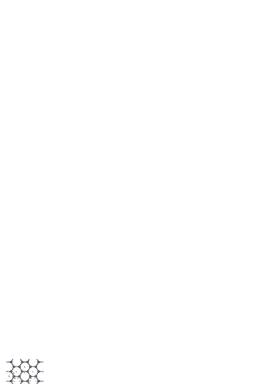
Figure 1: (Color online) Structure of H passivated 4ZGNR, where the dark grey and purple/light grey spheres represent the C and H atoms respectively. Labeling of carbon atoms across the ribbon with division into sublattices is introduced. The possible adatom locations: $h_{1}$, $h_{2}$, $h_{3}$ (hollow positions - most favorable), $t_{1}$, $t_{2}$ - top sites, $b_{1}$, $b_{2}$ - bridge positions and perturbed hollow like site of the edge $h_{0}$ are depicted.

Concerning the choice of the wave function basis set two codes have been employed: Vienna simulation package (VASP) VASP with the projector augmented wave basis sets (PAW) PAW and OPENMX, which uses basis set of localized pseudoatomic orbitals (LCPAOs) OPENMX . In the latter case for the geometrical optimization and the electronic band structure calculations the LCPAO basis functions were specified by the choice of two primitive orbitals for $s$ component and one primitive orbital for $p$ component for hydrogen ($H5.0-s2p1$) and three $p$ orbitals for carbon ($C5.0-s2p3$). The cutoff radius of $5.0$ Bohr has been assumed. VASP code is widely used, but due to the plane wave picture it is difficult to describe the effects of edges and to discuss field induced charge accumulation or dipole moments. In both codes the GGA-PBE exchange-correlation potential has been adopted PBE , which is specified not only by spin densities, but also by their gradients. In comparison with LSD GGA’s tend to improve total energies and structural difference PBE . In VASP, where smooth pseudopotentials are used a kinetic energy cutoff of $400$ eV was found to be sufficient to achieve a total energy convergence of the energies of the systems to within $1$ meV. In OPENMX real-space grid technique was adopted in numerical integration with energy cutoff up to $150$ Ry. In both methods the structures were relaxed until the Hellman-Feynman force became smaller than $10^{-4}$ Ha/bohr. Brillouin integration was carried out at $8\times 1\times 1$ Monkhorst-Pack grid and Gaussian smearing of $0.03$ eV was chosen to accelerate electronic convergence in both codes. For band structure calculations $50$ and $200$ uniform k points along the one-dimensional BZ were used in VASP and OPENMX respectively. To avoid interaction between images made by periodic boundary conditions the vacuum region was set up to $18$ Å in y- and up to $20$ Å in z-directions, in x-direction ribbon was treated as infinite. The adatom - ribbon system lacks inversion symmetry and therefore has a net electric magnetic moment perpendicular to the surface. To remove spurious dipole interaction between periodic images, we selfconsistently applied corrections to the local electrostatic potential and total energy Chan . To test an impact of correlations on the adsorption energy and magnetic moments we have performed also some GGA+U type calculations using rotationally invariant LDA+U functional proposed by Lichtenstein et al. Liechtenstein . The stability of adatom on the relaxed GNR was examined analyzing adsorption energy defined as:

$${\cal E}_{ads}={\cal E}_{{\cal{ZGNR}}+{\cal{C}}o}-{\cal E}_{{\cal{ZGNR}}}-{\cal E}_{{\cal{C}}o},$$ (1)

where the first term is total energy of ZGNR with Co adatom, and second and third are total energies of clean ZGNR and isolated Co atom.

II.2 Electronic and magnetic properties of ZGNR

It is now well established, that zigzag edge GNR is a semiconductor with two electronic edge states, which are ferromagnetically (F) ordered, but antiferromagnetically (AF) coupled to each other Kan1 ; Son ; Son2 . This configuration is consistent with the Lieb theorem Lieb . It is also well understood, that magnetism of the edges arises from a Fermi instability of the edges Gillen .

Table 1: Differences between energies of NZGNR states with antiparallel (AF) and parallel (F) alignment of magnetic moments on the left and right edges compared with corresponding differences of energies of AF and nonmagnetic states ($N=3-10$) (VASP).

${\cal{N}}$	${\cal{E}}_{{\cal{AF}}-{\cal{F}}}[meV]$	${\cal{E}}_{{\cal{AF}}-{\cal{NM}}}[meV]$
$3$	$-18.61$	$-39.01$
$4$	$-13.23(-14,-15,-11)$	$-55.74(-59)$
$5$	$-10.67$	$-65.10$
$6$	$-11.39(-11.9,-15)$	$-69.41(-85.7,-81)$
$7$	$-8.83(-11.2)$	$-71.64(-89.4)$
$8$	$-5.88(-8.4,-7)$	$-73.73(-91.8,-83)$
$9$	$-4.23$	$-75.75$
$10$	$-3.34(-5.5)$	$-77.47$

Our VASP calculations show that for $N=4$ the unpolarized solution has energy by $\Delta{\cal{E}}=55.74$ meV per edge carbon atom higher compared to AF state and $13.23$ meV higher than F state. The energy difference between parallel and antiparallel orientations of magnetizations at the edges decreases with the width (Tab. I) indicating that the increase of the overlap of edge states is responsible for relative ordering of polarizations. The obtained values are in good agreement with results reported by other groups.

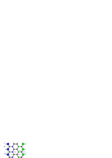
Figure 2: (Color online) Spin density plots of 4ZGNR showing up (blue/dark grey) and down (green/light grey) spin densities together with the corresponding values of local magnetic moments calculated with VASP code using a) GGA-PBE exchange correlation potential b) non-local GGA-HSE potential.

Fig. 2 compares spin densities plot of 4ZGNR calculated with local exchange potential (GGA-PBE) with corresponding picture obtained within non-local approach (HSE). Estimation of magnetic moment is sensitive to the choice of exchange potential, for non-local functional HSE (Fig. 2b) much higher values are obtained and slower decay towards the centre of the ribbon. These trends can be understood as a consequence of the well known property of non-local potentials, which localize electronic states more strongly compared to local potentials HSE ; Paier . It is clearly seen, that spin moments are mainly distributed at the edge carbon atoms. The magnetic moment fluctuation across the ribbon arises from quantum interference effects caused by edges. Due to topology of the lattice, the atoms of the two edges belong to different sublattices of the bipartite graphene lattice. The spin moments on the C atoms on one edge are antialigned to the spin moments on the opposite edge and also the polarizations of neighboring sites belonging to different sublattices are opposite. Figs. 3a, b present 4ZGNR bands calculated with VASP code decorated with local spin dependent edge contribution (overlap of the band eigenstates with $p_{z}$ state localized at ${\cal{A}}_{1}$). Two observations are striking, first that the top of the valence band and the bottom of the conduction band are composed mainly of edge states, especially close to the zone boundary and second that in momentum range $2\pi/3a<k<\pi/a$ ($a$ is ZGNR lattice constant) lowest unoccupied conduction band (LUCB) and the highest occupied valence band (HOVB) are characterized by opposite spin polarizations. Of course for the right edge (${\cal{B}}_{4}$) the spin contributions change the roles. We have also marked in Fig. 3 the direct band gap ($\Delta_{0}$) and the energy gap at the zone boundary ($\Delta_{1}$).

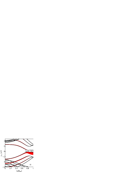
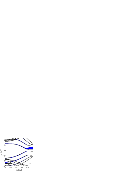
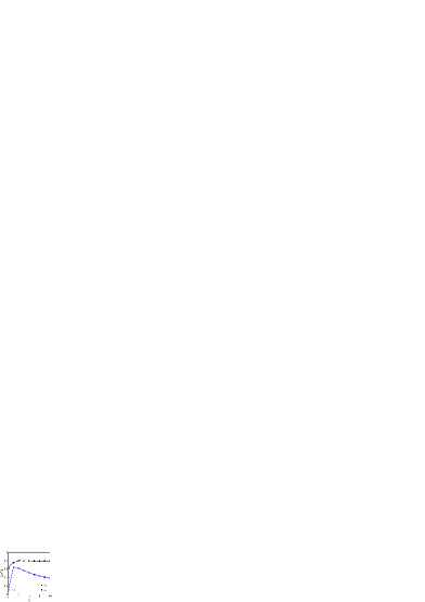
Figure 3: (Color online) a, b) VASP spin degenerate bands of 4ZGNR with fat bands showing the amplitudes of the projection of each band on $p_{z}$ orbital of edge atom ${\cal{A}}_{1}$. $\Delta_{0}$ and $\Delta_{1}$ are direct band gap and gap of the zone boundary c) dependence of the gap on the nanoribbon width.

The magnetization induced staggered potential opens a band gap. The direct band gap decreases with the increase of the width of the ribbon due to confinement and decrease of edge spin polarization (Fig. 3c).

Figure 4: (Color online) Electric field dependencies of energy gap of 4ZGNR for spin up (lower black curves) and spin down (upper blue curves) calculated with the use of VASP code (dashed lines) and OPENMX (solid lines). Inset shows the corresponding dependencies for 6ZGNR.

The energy gap at the zone boundary on the other hand is almost not sensitive to the width, because as stated earlier, the edge states close to the zone boundary are highly confined at the edge of ZGNR. It is known, that local or semilocal approximations such as GGA routinely underestimate semiconductor band gaps, due to self-interaction errors Paier . For comparison we have also calculated the band gap with HSE potential, the obtained value is surprisingly high ($\Delta_{HSE}=1.58$ eV for 4ZGNR) but agrees with other HSE calculation Xiang . It is general accepted, that band gaps obtained using hybrid functionals are in much better agreement with experimental data, although overestimated Kummel ; Barone .

II.3 Evolution of electronic structure with electric field

Existence of edge states in ZGNR gives a possibility to tune the electronic and magnetic properties of these systems and bellow we discuss one way of such modification, the effect of electric field. The external transverse field is simulated in our calculations by a periodic saw-tooth type potential Son , which is perpendicular to the ribbon edge.

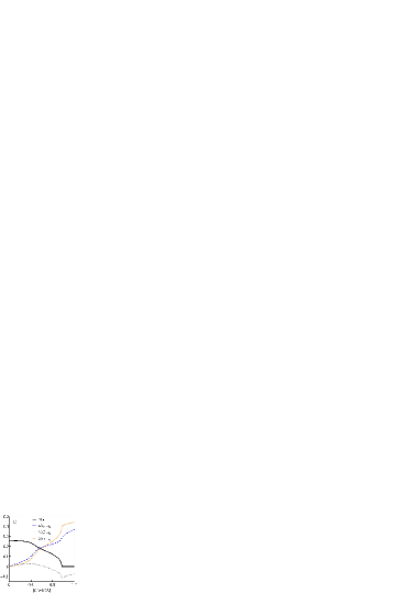
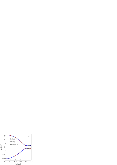
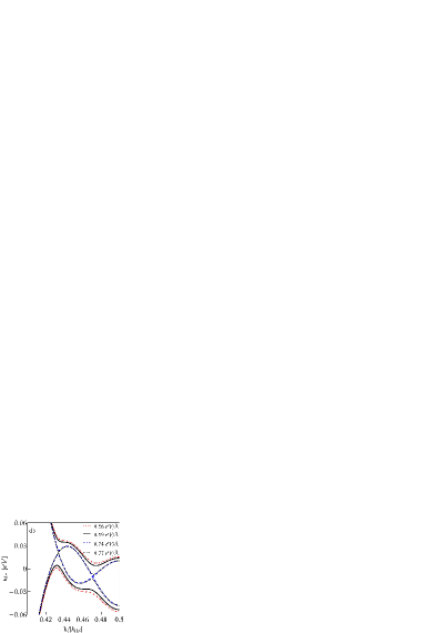
Figure 5: (Color online) a) Electric field dependence of edge magnetic moment of ${\cal{A}}_{1}$ atom in 4ZGNR (black solid line) together with charge transfer from right to the left edge $\Delta{\cal{N}}_{{\cal{A}}_{1}-{\cal{B}}_{4}}$ (dashed blue line) and corresponding spin up (grey dashed-dot dot line) and spin down (dotted line) contributions to the charge transfer (OPENMX). b) Field evolution of edge magnetic moments of 4ZGNR (solid black line), 6ZGNR (dotted blue line) and 10ZGNR (dashed red line). Inset compares the field evolution of the gaps for the same choice of nanoribbon widths. c) Comparison of LUCB and HOVB bands of 4ZGNR (OPENMX) of zero field case with finite field $|E|=0.1$ eV/Å. d) The zoom-view of spin up LUCB and HOVB in the narrowed momentum range for representative fields in the vicinity of critical field which closes the gap.

Field evolution of the gaps obtained by VASP and OPENMX methods are depicted on Figure 4. With the increase of electric field, the spin-down band gap decreases and becomes zero for electric field strength depending on the ribbon width. The critical field to achieve half-metallicity decreases with increasing width. The spin-up channel remains semiconducting under all external fields. In agreement with earlier results Son ; Kan2 , our calculations predict that half-metallicity will be destroyed by a too strong electric fields. According to OPENMX the electric field range at which ZGNR remains half-metallic increases with the ribbon width (Fig. 4 and inset of Fig. 5b), in VASP calculations this range is very narrow. The observed differences are probably due to the different choice of the wave function basis sets and consequently different treatment of screening in both codes. As suggested by Son Son , the half-metallicity comes from the relative movement in energy of edge states under electrostatic potential, oppositely for a given spin direction on left and right edges. The field evolution of edge magnetic moment and the charge difference between the edges of 4ZGNR are presented on Fig. 5a. The charge transfer from one edge into the opposite edge suppresses the edge moments and for high enough fields the moments vanish. The charge imbalance between spin up electron from left and right edges is suppressed ($\Delta{\cal{N}}^{+}_{{\cal{A}}_{1}-{\cal{B}}_{4}}=0$) for the field $|E|=0.59$ eV/Å, when spin up LUCB and HVOB bands start to overlap (Fig. 5d). For higher fields, when the overlap increases the charge transfer $\Delta{\cal{N}}^{+}_{{\cal{A}}_{1}-{\cal{B}}_{4}}$ changes sign (Fig. 5a). Fig. 5b compares the electric field dependencies of edge magnetic moments for different nanoribbon widths. Figs 5c, d show the representative VASP dispersions of low energy bands for the selected values of the field. It is seen that in the interesting momentum range $2\pi/3a<k<\pi/a$ the LUCB and HOVB bands for one spin direction become closer and their curvatures undergo reconstruction due to the effect of the screened electric field. In the range of extremely narrow gap, where the electric field mixes the occupied states with unoccupied ones the single minimum (LUCB) or maximum (HOVB) evolves into a pair of close minima or maxima and the bands come close to the Fermi level asymmetrically. The evolution of these bands is affected by coupling of edges, which depends on interference and confinement effects. Our calculations suggest that HOVB crosses the Fermi level first, for fields slightly smaller than the critical fields required for closing the gap. Since the rest of the paper focuses only on the zero field case, we postpone more elaborated analysis of the field dependence of the nanoribbon electronic structure for our future publication.

II.4 Co adatom

The computational tools we use (VASP, OPENMX) are developed for periodic structures and therefore we simulate the single impurity problem by superstructure calculations. As a consequence of periodicity the extra features in the generated band structure can occur e.g. additional gaps not related to finite geometry, but to the assumed superstructure.

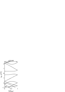
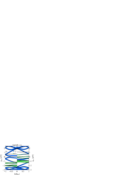
Figure 6: (Color online) VASP energy dispersion curves of 4ZGNR compared with the bands of 4ZGNR with Co impurity in $h_{1}$ position. The blue/dark grey fat bands highlight carbon $p_{z}$ contribution and green/light grey the Co $d$ contribution.

It is believed however, that using large enough supercells one can still infer about some single impurity properties. This concerns mainly quantities which depend on the entire density of states and not just on the behavior near the Fermi level, e.g. occupations or magnetic moments. With some caution one can get also an insight into some parts of the electronic structure, where superstructure does no interfere considerably. In our study we use a supercell consisting of four replicas of ZGNR unit cell ($4\times 1$). This setup corresponds to a coverage of $1$ adatom per $32$ C atoms. Although the adatom-adatom interaction is not negligible, the distance between adatoms is large enough that the overlap of the electronic states of neighboring atoms is negligible. Several test simulations were also carried out for a $8\times 1$ supercell. Periodic boundary conditions were also used along confined direction assuming $20$ Å of vacuum to prevent unphysical interactions. Different positions, as indicated on Fig. 1 were sampled. Fig. 6 presents an example of the band structure of 4ZGNR$+$Co system with adatom in $h_{1}$ position compared with the band structure of pure nanoribbon. The bands are decorated by the amplitudes of the projection on atomic $p_{z}$ orbitals of carbon and Co $d$ orbitals. The strong interaction between cobalt and carbon atoms comes from the mixture of these states. Carbon $p_{x}$ and $p_{y}$ orbitals are far below ${\cal{E}}_{{\cal{F}}}$ and have weak hybridization with cobalt.

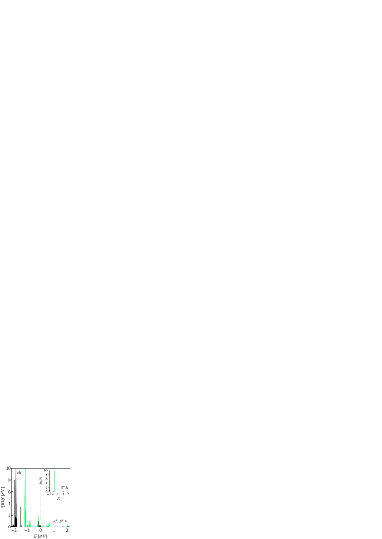
Figure 7: (Color online) Spin and orbital resolved densities of states of Co adatom at $h_{1}$ position in 4ZGNR. The black denote spin up contributions and green/light grey the spin down contributions. Inset of Figs. b, c present $yz$ and $xy$ partial DOS of Co adatom at $h_{0}$ site.

Fig. 7 displays the corresponding spin and orbital resolved Co adatom densities of states. In pure graphene, in consequence of $C_{6v}$ point symmetry the $4s$ and $3d_{z}^{2}$ orbitals do not hybridize with graphene orbitals close to the Dirac points. In nanoribbon this symmetry is broken, but still hybridization of these orbitals is only very weak. The rest of Co $d$ orbitals hybridize strongly, what results in covalent interactions. The bonding, almost completely occupied orbitals $d_{x^{2}-y^{2}}$ , $d_{xy}$ lie lower in energy than $d_{xz}$ and $d_{yz}$, the latter are partially filled and they play an active role in formation of magnetic moment. Depending on the position of adatom some orbitals may swap the roles. This can be seen comparing for example the $d_{xy}$ , $d_{yz}$ , partial DOS for $h_{1}$ and $h_{0}$ sites (Figures 7b, c).

Table 2: Illustration of the impact of Coulomb interaction and exchange interaction on the values of adsorption energies of Co adatom in hollow positions of 4ZGNR (GGA+U) Liechtenstein .

	${\cal{E}}_{ads}^{h_{1}}[eV]$	${\cal{E}}_{ads}^{h_{2}}[eV]$
${\cal{U}}=0$ ${\cal{J}}=0$	$-1.60$	$-1.37$
${\cal{U}}=2$ ${\cal{J}}=0$	$-1.06$	$-0.76$
${\cal{U}}=4$ ${\cal{J}}=0$	$-0.93$	$-0.84$
${\cal{U}}=2$ ${\cal{J}}=0.9$	$-1.20$	$-0.87$
${\cal{U}}=4$ ${\cal{J}}=0.9$	$-1.14$	$-0.87$

For $h_{0}$ position $d_{yz}$ orbital becomes fully occupied whereas $d_{xy}$ shifts closer to ${\cal{E}}_{{\cal{F}}}$ and takes over the role of magnetic orbital. The reversal of the roles is a consequence of the change of symmetry and reduced coordination, what alters hybridization amplitudes (see hybridization Tab. IV) and consequently modifies the widths and effective orbital splittings of $4d$ levels.

Figure 8: (Color online) Total energy curves for different positions of Co adatom on 4ZGNR. Inset is the zoom-view of spin resolved energy curves for $h_{1}$ position presented close to minimum.

To understand the energetics of Co adsorption on graphene nanoribbon we performed a series of calculations for different vertical distances of Co and nanoribbon plane. The calculated equilibrium heights of adatom together with adsorption energies are summarized in Tab. III and Figure 8 presents selected adsorption energies curves.

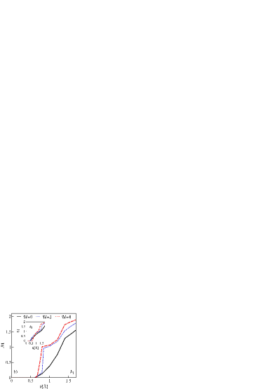
Figure 9: (Color online) a) GGA+U estimations of total magnetic moment of Co impurity in 4ZGNR for diffrent values of Coulomb interaction parameter. The dots represent additional effects of exchange (${\cal{J}}=0.9$ eV) for $h_{0}$ (circle), $h_{1}$ (square) and $h_{2}$ (triangle). Inset shows the total energy curves for $h_{1}$ position for selected values of ${\cal{U}}$. b) Adatom-graphene nanoribbon distance dependence of total magnetic moment of Co impurity for $h_{1}$ and $h_{2}$ (inset) positions.

The formed covalent bonds are directional and the bond strength depends on the adatom coordination. Therefore it is unsurprising that the adsorption energy is strongly dependent on the adsorption site. The presented energies are the minimal values obtained after relaxation.

Table 3: Equilibrium heights above nanoribbon plane and adsorption energies of Co adatom at different positions of 4ZGNR (VASP with GGA-PBE).

$-$	$h_{eq}[$Å$]$	${\cal{E}}_{ads}[eV]$
$h_{0}$	$1.7$	$-1.261$
$h_{1}$	$1.53$	$-1.396$
$h_{2}$	$1.53$	$-1.158$
$t_{1}$	$1.83$	$-0.341$
$t_{2}$	$1.85$	$-0.407$
$b_{1}$	$1.79$	$-0.946$
$b_{2}$	$1.85$	$-0.477$

Since nanoribbon polarization is nonuniform, adsorbsion energy depends on Co spin polarization, but as shown in the example of $h_{1}$ position (inset of Fig. 8), the adsorption curves for different spin orientations do not differ significantly. Nevertheless the predicted spin orientations of Co adatoms deposited at $h_{1}$ and $h_{3}$ positions are opposite, whereas at the ribbon center, where no net magnetic polarization of ZGNR occurs the energies for both Co spin orientations are degenerate. Co adatom prefers hollow positions, where the impurity is not associated with a particular sublattice, but instead binds three carbon atoms from each. Following Power et al. Power we have also checked that at the edge a new type of metastable adsorption site is realized ($h_{0}$, Fig. 1), where impurity connects to three edge zigzag atoms. This position is however only reached after relaxation along the path starting from adatom originally siting at $t_{1}$ or $t_{2}$ positions.

Table 4: Nearest neighbors hybridization amplitudes of Co adatom located in hollow positions of 4ZGNR.

	$h_{0}$		$h_{1}$				$h_{2}$
$d$	$|{\cal{V}}^{{\cal{A}}_{1}}_{d}|$	$|{\cal{V}}^{{\cal{B}}_{1}}_{d}|$	$|{\cal{V}}^{{\cal{A}}_{1}}_{d}|$	$|{\cal{V}}^{{\cal{A}}_{2}}_{d}|$	$|{\cal{V}}^{{\cal{B}}_{1}}_{d}|$	$|{\cal{V}}^{{\cal{B}}_{2}}_{d}|$	$|{\cal{V}}^{{\cal{A}}_{2}}_{d}|$	$|{\cal{V}}^{{\cal{A}}_{3}}_{d}|$	$|{\cal{V}}^{{\cal{B}}_{2}}_{d}|$	$|{\cal{V}}^{{\cal{B}}_{3}}_{d}|$
$z^{2}$	$0.13$	$0.64$	$0.001$	$0.001$	$0.001$	$0.001$	$0.001$	$0.001$	$0.001$	$0.001$
$xz$	$0.47$	$0$	$0$	$0.68$	$0.66$	$0$	$0$	$0.67$	$0.67$	$0$
$yz$	$0.13$	$0.65$	$1.92$	$0.59$	$0.59$	$1.87$	$1.81$	$0.55$	$0.55$	$1.81$
$xy$	$0.47$	$0$	$0$	$0.28$	$0.28$	$0$	$0$	$0.28$	$0.28$	$0$
$x^{2}-y^{2}$	$0.3$	$0.52$	$0.79$	$0.25$	$0.21$	$0.76$	$0.78$	$0.25$	$0.25$	$0.78$

Taking into account electron correlations is crucial for the description of adsorption of transition metal atoms. Here we present in Tab. II some testing results obtained within GGA + U type approach. The estimated adsorption energy significantly lowers with the increase of ${\cal{U}}$ whereas ${\cal{J}}$ enhances it. Inset of Fig. 9a illustrates that for higher values of Coulomb interaction the equilibrium distance of Co adatom increases. Table VI presents GGA-PBE orbital occupations and total and orbital contributions to magnetic moments of Co for $h_{0}$, $h_{1}$ and $h_{2}$ positions, which correspond to the earlier presented local densities of states (Fig. 7). Magnetic moments of Co at the ZGNR depend on the adsorption site, but their absolute value in all cases are much smaller than the moment of the free atom (${\cal{M}}_{Co}\approx 3\mu_{B}$ Jacob ). The decrease of magnetic moment is dictated by electron transfer from $4s$ to $3d$ states and corresponding change of occupancy of the unpaired $3d$ orbitals. The spin-down component of the hybrid states is almost entirely below ${\cal{E}}_{{\cal{F}}}$, while a large amount of the spin-up component lies above ${\cal{E}}_{{\cal{F}}}$. As aforementioned, in the case of hollow sites moments come mainly from $d_{xz}$ and $d_{yz}$ orbitals and their contributions are $1.103$ and $0.941$ for $h_{1}$ and $h_{2}$ respectively, i.e. they do not differ much from unity. We have checked that the trend of decrease of moment with moving with the adsorption site to the centre of the ribbon persists in wider ribbons and for ${\cal{N}}=10$ total magnetic moment reaches at the center ${\cal{M}}=1.094$ what is close to the value for Co adatom on graphene (${\cal{M}}=1.083$). Similarly binding energy in the center of a wide ribbon converges to the value for graphene ${\cal{E}}_{ads}=-1.23$ eV, already for ${\cal{N}}=8$ amounts value ${\cal{E}}^{h_{4}}_{ads}=-1.37$ eV.

It is known that pure LDA approach inaccurately estimates magnetic moments and therefore we present in Fig. 9 how the results are modified by inclusion of correlations within GGA+U scheme. The finite ${\cal{U}}$ solutions give larger values of estimated magnetic moments and Hund’s coupling reduces the moment and diminishes the difference of $d_{xz}$ and $d_{yz}$ contributions.

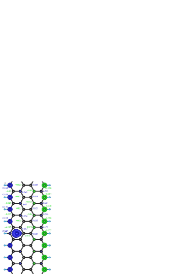
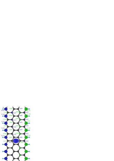
Figure 10: (Color online) Spin density plots of Co adatom and 4ZGNR matrix ($8\times 1$ supercell). The blue/dark grey densities correspond to spin up and green/light grey to spin down components. a) Co impurity in $h_{1}$ position b) Co in $h_{2}$ position.

We also present in Fig. 9 magnetic moments dependencies of Co adatom on the height for three values of Coulomb interaction parameter and Fig. 9a, b compares distance dependencies for $h_{1}$ and $h_{2}$ positions. Increase of the overlap of impurity to ribbon states with decrease of the distance results in a reduction of magnetic moment. Close to nanoribbon surface the occupation of weakly hybridized $4s$ state is less favorable than these of strongly hybridizing $3d$ orbitals. Hybridization lowers the energy of the orbitals and due to increased delocalization the Coulomb repulsion is reduced. In consequence of $4s-3d$ charge transfer the decrease of magnetic moment results.

Table 5: Total magnetic moments of Co atoms located in hollow positions of NZGNR ($N=4,6,8$) compared with magnetic moment of Co at hollow site of graphene (VASP with GGA-PBE).

	${\cal{M}}$	${\cal{M}}_{h_{1}}$	${\cal{M}}_{h_{2}}$	${\cal{M}}_{h_{3}}$	${\cal{M}}_{h_{4}}$
${\cal{G}}+{\cal{C}}o$	$1.083$	$-$	$-$	$-$	$-$
$4{\cal{ZGNR}}+{\cal{C}}o$	$-$	$1.413$	$1.178$	$-$	$-$
$6{\cal{ZGNR}}+{\cal{C}}o$	$-$	$1.383$	$1.209$	$1.122$	$-$
$8{\cal{ZGNR}}+{\cal{C}}o$	$-$	$1.376$	$1.258$	$1.180$	$1.115$

Figures 10a, b. show the spin polarization patterns induced by the presence of Co adatom at $h_{1}$ and $h_{2}$ sites calculated for $8\times 1$ supercell. For the twice reduced supercell ($4\times 1$) the local polarizations around impurity are almost identical to $8\times 1$ case, the differences are only seen at the border of supercells. In the case of $4\times 1$ cell the edge magnetic moments at a grater distance from impurity do not approach the values for pure nanoribbon, this is achieved for $8\times 1$ cell. As it is seen from Fig. 10 the polarization effect is strongest for Co located in $h_{1}$ position and nearest edge atoms are most sensitive to perturbation. Our calculations indicate the charge transfer from Co to the $\pi$ bands of nanoribbon and no transfer is observed to the $\sigma$ bands. The occupation of the neighboring carbon $p_{z}$ orbitals is increased with adsorption and the spin polarization of the nearby atoms at the edge is locally suppressed.

III KONDO EFFECT OF CO ATOM ON HOLLOW SITE

III.1 Model

Static mean field DFT description of the electronic structure of Co adsorbed on the nanoribbon does not capture the effects of dynamic correlations of strongly interacting $3d$ electrons. To complement the missing local correlations of adatom electrons we complete the model by Hubbard type term and exchange Pruschke1 ; Makarovski . The description of nanoribbon substrate and its coupling to impurity is maintained within DFT formalism. The Kohn-Sham Hamiltonian thereby serves as the non-interacting reference frame onto which we add local intra-atomic interactions. As we have presented in the preceding chapter, in the case of the considered hollow location of Co atom the $d_{xz}$ and $d_{yz}$ orbitals are responsible for formation of magnetic moment, their fluctuations in occupations and spins are essential for low energy physics. We discuss therefore double orbital Anderson-like Hamiltonian in the form:

$${\mathcal{H}}={\mathcal{H}}_{d}+{\mathcal{H}}_{v}+{\mathcal{H}}_{{\cal{ZGNR}}},$$ (2)

where impurity is described by

$${\mathcal{H}}_{d}=\sum_{m\sigma}\varepsilon_{0}n_{m\sigma}+{\cal{U}}\sum_{m}n_{m+}n_{m-}+({\cal{U}}-{\cal{J}}/2)n_{m}n_{m^{\prime}}$$

$$-2{\cal{J}}\overrightarrow{{\cal{S}}}_{m}\cdot\overrightarrow{{\cal{S}}}_{m^{\prime}}$$ (3)

and $\varepsilon_{0}$ is the bare energy of local levels, assumed to be equal for both orbitals, ${\cal{U}}$ is the energy of intra or interorbital Coulomb interaction and ${\cal{J}}$ is Hund’s exchange coupling. Nanoribbon Hamiltonian reads:

$${\mathcal{H}}_{{\cal{ZGNR}}}=\sum_{kn\sigma}{\epsilon}_{kn\sigma}c^{{\dagger}}_{kn\sigma}c_{kn\sigma},$$ (4)

Table 6: Magnetic moments and spin occupancies of different Co orbitals for hollow positions of 4ZGNR (VASP).

	$h_{0}$			$h_{1}$			$h_{2}$
$d$	${\cal{N}}_{+}$	${\cal{N}}_{-}$	${\cal{M}}$	${\cal{N}}_{+}$	${\cal{N}}_{-}$	${\cal{M}}$	${\cal{N}}_{+}$	${\cal{N}}_{-}$	${\cal{M}}$
$z^{2}$	$0.966$	$0.933$	$0.033$	$0.997$	$0.994$	$0.003$	$0.996$	$0.989$	$0.007$
$xz$	$0.963$	$0.456$	$0.507$	$0.963$	$0.503$	$0.46$	$0.937$	$0.729$	$0.208$
$yz$	$0.955$	$0.889$	$0.066$	$0.979$	$0.336$	$0.643$	$0.978$	$0.245$	$0.733$
$xy$	$0.997$	$0.062$	$0.935$	$0.934$	$0.837$	$0.097$	$0.905$	$0.845$	$0.06$
$x^{2}-y^{2}$	$0.965$	$0.926$	$0.039$	$0.892$	$0.763$	$0.129$	$0.879$	$0.782$	$0.097$
$tot$	$-$	$-$	$1.579$	$-$	$-$	$1.332$	$-$	$-$	$1.105$

with $\varepsilon_{kn\sigma}$ denoting DFT ribbon eigenvalues and corresponding eigenfunctions $|kn\sigma\rangle$. The interaction between nanoribbon electrons and local levels is described by hybridization term:

$${\mathcal{H}}_{v}=\sum_{kn\sigma m}({\cal{V}}_{kn\sigma m}c^{{\dagger}}_{kn\sigma}d_{m\sigma}+h.c.),$$ (5)

where hybridization amplitudes $V_{kn\sigma m}$ are hopping matrix elements between nanoribbon DFT eigenstates and $d$ orbitals. In this work, the realistic ab initio hybridization is taken from GGA-PBE calculations based on VASP code. Hybridization strengths we use are not strictly single impurity couplings due to the periodicity of the adopted first principles computations schemes, but for large enough supercells they can approximately play this role. The nearest neighbor impurity-nanoribbon hopping integrals are extracted from DFT data $V^{i}_{m}=\sum_{kn}\langle d_{m}|\overline{kn}\rangle\overline{\varepsilon_{kn}}\langle\overline{kn}|p^{i}_{z}\rangle$,where $|m\rangle$ denotes adatom orbital, $|\overline{kn}\rangle$ and $\overline{\varepsilon_{kn}}$ are DFT eigenstates and energies of $Co+ZGNR$ system.

Table IV presents hybridization amplitudes in real space with restriction to the dominant n.n. contributions. For comparison we present amplitudes for all $3d$ orbitals. Note the smallness of the amplitudes to $A_{1}$ and $B_{2}$ for $d_{xz}$ in $h_{1}$ position and large amplitudes to these atoms for $d_{yz}$. Pictorially this difference can be understood recalling the shapes of these orbitals. Remembering that the edge states dominate the energy window near the gap, one can expect distinctly different roles of $d_{xz}$ and $d_{yz}$ orbitals in Kondo physics for $h_{1}$ position. For $h_{2}$ the role of edge states is diminished. Comparison of the amplitudes for $h_{0}$ and hollow sites helps to understand the earlier mentioned reversal of the role between $d_{yz}$ and $d_{xy}$ when positions of the adatom interchange.

To describe orbital degrees of freedom on the same footing as spin it is useful to introduce orbital pseudospin ${\cal{T}}$ defined by ${\cal{T}}=\Psi_{d}^{{\dagger}}\tau\Psi_{d}$, where $\tau$ is Pauli matrix in orbital space $\{d_{xz},d_{yz}\}$ and $\Psi_{d}^{{\dagger}}$ represents spin-orbital field operator $\Psi_{d}^{{\dagger}}=[d^{{\dagger}}_{xz+},d^{{\dagger}}_{xz-},d^{{\dagger}}_{yz+},d^{{\dagger}}_{yz-}]$.

III.2 Hybridization function

Hybridization function describes coupling of impurity to nanoribbon. Hereafter we restrict to nearest neighbors of impurity and consider only $d_{xz}$ and $d_{yz}$ orbitals. Hybridization then reads:

$$\Sigma^{h_{1(2)}}_{mm^{\prime}\sigma}=\sum_{kn}\frac{V^{*h_{1(2)}}_{kn\sigma m}V^{h_{1(2)}}_{kn\sigma m^{\prime}}}{z-\varepsilon_{kn\sigma}},$$ (6)

where $\varepsilon_{kn\sigma}$ and $|kn\sigma\rangle$ are DFT eigenenergies and eigenstates of bare graphene nanoribbon and $V_{kn\sigma m}=(1/\sqrt{N_{x}})\sum_{l_{h}}\sum_{a_{h}}V^{a_{h}}_{m}e^{ika_{h}}\langle kl_{h}\sigma|kn\sigma\rangle$, where $a_{h}$ are n. n. vectors connecting adatom with carbon sites from surrounding hexagon, $l_{h}$ labels four carbon chains along infinite $x$ direction crossing the hexagon, $N_{x}$ is the number of sites in carbon chain in $x$ direction and $|kl\rangle=(1/\sqrt{N_{x}})\sum e^{iki_{l}}|p^{i_{l}}_{z}\rangle$. All hybridization functions presented below have been calculated using VASP code.

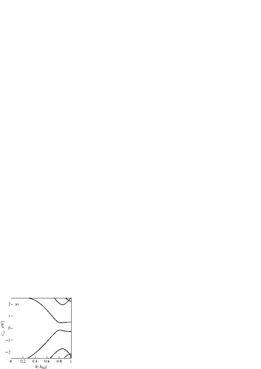
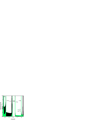
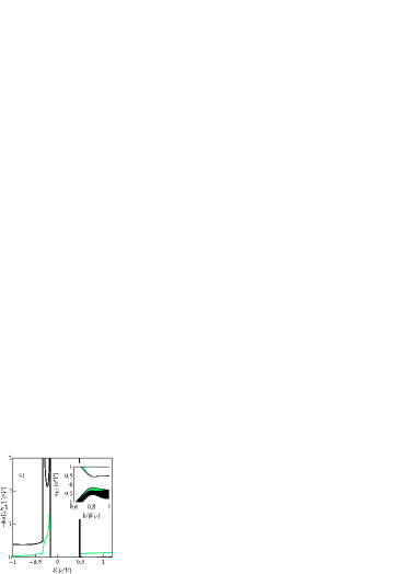
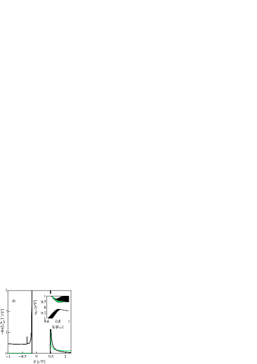
Figure 11: (Color online) Low energy band structure of 4ZGNR (a) together with orbitally resolved hybridization functions of Co adatom in $h_{1}$ position (b, c, d). Black color denotes $yz$ contribution and geen/light grey $xz$. In Fig. b labeling of Van Hove singularities used further in the text is introduced. Figures c, d present spin up and spin down parts of hybridization respectively. Insets of Figs. c, d are zoom views of lowest dispersion curves decorated with $xz$ and $yz$ contributions.

For pure graphene $\Sigma_{mm^{\prime}}\sim\delta_{mm^{\prime}}$ due to $C_{6v}$ symmetry of hollow sites. In nanoribbon, where this symmetry is broken also off-diagonal terms occur, but as we have checked due to rapid oscillations in k-space they are much smaller than diagonal elements and additionally they affect the impurity states in forth power in hybridization, whereas the diagonal in second power. Based on these arguments we neglect in the following, for simplicity of calculations, the off-diagonal self energies. Hybridization function plays the role of embedding self-energy. The real parts of self-energies are associated with the shift of the local energies, while the imaginary parts give the broadening of impurity levels. Fig. 11 shows imaginary part of the low energy hybridization functions for $h_{1}$ position together with the corresponding VASP nanoribbon bands from this range. In the following we refer to the presented singularities and therefore we introduce their labeling in Fig. 11b. More detailed pictures of spin and orbital resolved hybridization with both real and imaginary parts are presented in Fig. 12. In general the hybridization functions are spin dependent, what is mainly dictated by spin dependence of local nanoribbon Green’s functions. The opposite local polarizations at $h_{1}$ and $h_{3}$ (Fig. 1) reflects in the change of roles of spins in hybridization function $\Sigma^{h_{1}}_{m\sigma}=\Sigma^{h_{3}}_{m\overline{\sigma}}$. At $h_{2}$, where polarization contributions from the opposite edges compensate hybridizations are equal for both spin orientations. The hybridization functions are rich in structure, of special importance for Kondo effect are observed Van Hove singularities (VHS’s) occurring in position of minima, maxima or saddle points of the bands. Vanishing of derivatives of dispersion curves indicates energies, where singularities are expected, but whether singularity clearly reflects in orbital resolved hybridization depends on the weight of contribution of a given symmetry to the bands in the considered energy range. This fact is illustrated in Figs. 11 c, d, where highest conduction and lowest valence bands are decorated by amplitudes specifying projection of the eigenfunctions onto the symmetry of a given local orbital.

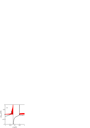
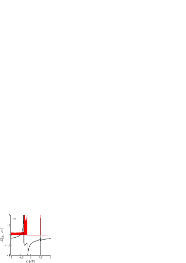
Figure 12: (Color online) Orbital and spin resolved hybridization functions for Co at $h_{1}$ position in 4ZGNR. Solid black lines represent real parts ($Re[\Sigma^{h_{1}}_{m\sigma}]$) and imaginary parts ($Im[\Sigma^{h_{1}}_{m\sigma}]$) are shown by green/light grey filled curves.

For example in the energy window presented in Figs. 11c, d two pronounced singularities are observed (${\cal{VH}}1\nu$ and ${\cal{VH}}2\nu$) below the gap for $yz$ symmetry, characterized by peaks in imaginary parts of hybridizations and discontinuities in real parts. For $xz$ symmetry on the other hand, similar behavior is seen only close to the gap.

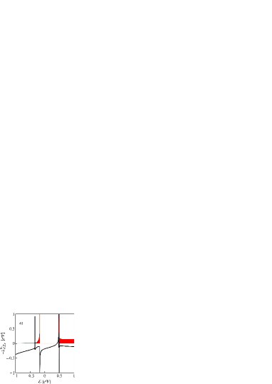
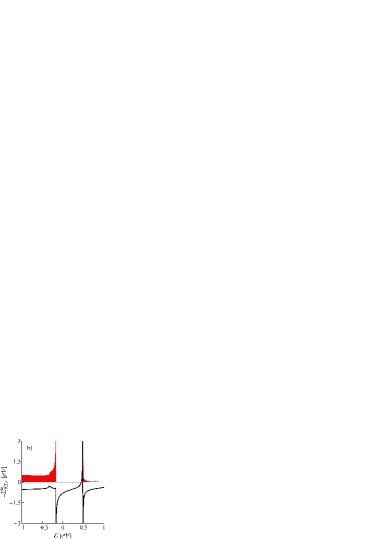
Figure 13: (Color online) Orbital resolved hybridization function of Co in $h_{2}$ position of 4ZGNR. Solid black lines represent real part and green/light grey filled curves show the imaginary parts of hybridization.

For ${\cal{E}}=-0.3348$ (${\cal{VH}}2\nu$) the $xz$ contribution to the bands is small (see the insets of Fig. 11c, d). The character of many-body resonances are determined by the deepness of the local level with respect to the Fermi energy and hybridization strength, both of these values dramatically change near the singularity and therefore it is expected, that an interesting physics emerges in the vicinity of these energy points.

III.3 Slave boson mean field approach

The described modeling of single adatom embedded onto graphene nanoribbon by Anderson like Hamiltonian allows us to examine the strong correlations by the well elaborated techniques with known applicability regimes. Our main interest focuses on the impact of the details of nanoribbon electronic and magnetic structure on the single impurity Kondo effect.

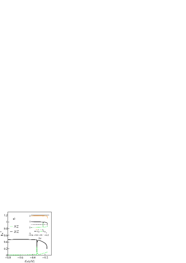
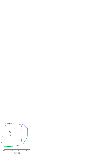
Figure 14: (Color online) Expectation values of slave boson operators, polarizations and expectation values of orbital pseudospin of Co impurity at $h_{2}$ position of 4ZGNR a) triple occupation slave boson operators $|t_{m}|^{2}=|t_{m+}|^{2}=|t_{m-}|^{2}$ b) double and full occupation slave boson operators $|d_{{\cal{T}}0}|^{2}$, $|d_{{\cal{T}}1}|^{2}$, $|d_{{\cal{T}}\overline{1}}|^{2}$, $|d_{{\cal{S}}1}|^{2}=|d_{{\cal{S}}\overline{1}}|^{2}$, $|d_{{\cal{S}}0}|^{2}=|d_{{\cal{T}}0}|^{2}$ and $|f|^{2}$ c) orbital polarization of Co at $h_{2}$ site (${\cal{P}}_{{\cal{O}}}=\frac{\varrho_{xz}({\cal{E}}_{\cal{F}})-\varrho_{yz}({\cal{E}}_{\cal{F}})}{\varrho_{xz}({\cal{E}}_{\cal{F}})+\varrho_{yz}({\cal{E}}_{\cal{F}})}$, where $\varrho_{m}({\cal{E}})=\sum_{\sigma}\varrho_{m\sigma}({\cal{E}})$ and $\varrho_{m\sigma}$ denotes spin-orbital partial density of states) and expectation value of Co orbital pseudospin (${\cal{T}}_{z}$). Inset of Fig. a shows total, spin and orbital ${d_{xz},d_{yz}}$ occupancies.

The basic analysis of variation of many-body correlations with tuning the chemical potential is based on mean field slave boson approach of Kotlar and Ruckenstein Ruckenstein . This approximation concentrates exclusively on many-body resonances taking into account spin and orbital fluctuations, but neglecting charge fluctuations. In principle SBMFA strictly applies close to the unitary Kondo limit, but due to its simplicity this method is also often used for systems with broken symmetry Bulka ; Lim ; Lipinski ; Trocha . It is believed that it captures the essential features of the examined problem also in this case. SMBFA is unreliable for higher temperatures.

Table 7: Two electron eigenstates of hamiltonian (3) with the assigned slave bosons.

$eigenstate$	$slave-boson$
$|\uparrow,\uparrow\rangle$	$d_{{\cal{S}}=1{\cal{S}}_{z}=1}=d_{{\cal{S}}1}$
$(1/\sqrt{2})(|\uparrow,\downarrow\rangle+|\downarrow,\uparrow\rangle)$	$d_{{\cal{S}}=1{\cal{S}}_{z}=0}=d_{{\cal{S}}0}$
$|\downarrow,\downarrow\rangle$	$d_{{\cal{S}}=1{\cal{S}}_{z}=\overline{1}}=d_{{\cal{S}}\overline{1}}$
$|\uparrow\downarrow,0\rangle$	$d_{{\cal{T}}=1{\cal{T}}_{z}=1}=d_{{\cal{T}}1}$
$(1/\sqrt{2})(|\uparrow,\downarrow\rangle-|\downarrow,\uparrow\rangle)$	$d_{{\cal{T}}=1{\cal{T}}_{z}=0}=d_{{\cal{T}}0}$
$|0,\uparrow\downarrow\rangle$	$d_{{\cal{T}}=1{\cal{T}}_{z}=\overline{1}}=d_{{\cal{T}}\overline{1}}$

This is a consequence of break of the required gauge invariance which is associated with charge conservation, what leads to artificial sharp transition to the state with vanishing expectation value of boson fields Hewson .

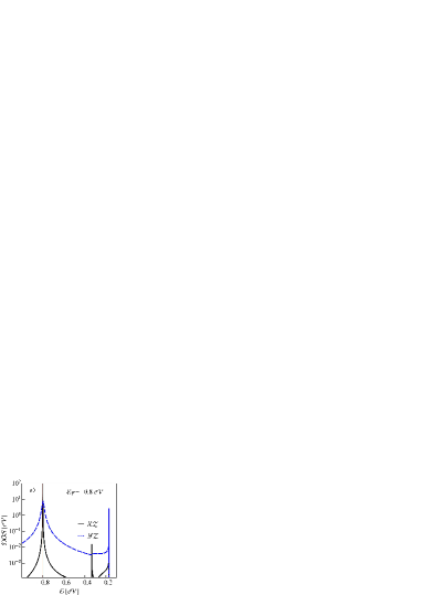
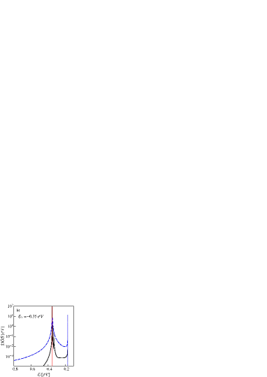
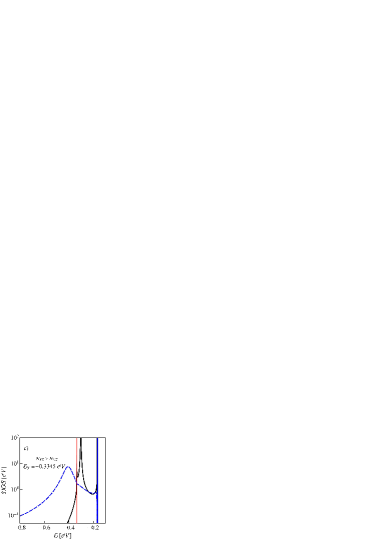
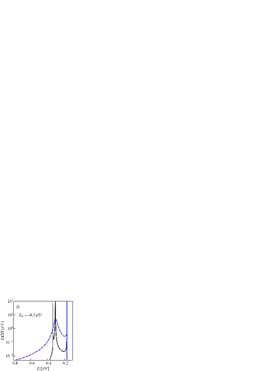
Figure 15: (Color online) Selected partial orbital DOS of Co at $h_{2}$ site in 4ZGNR. The vertical red/thin lines indicate positions of Fermi levels.

To get some insight into the higher temperatures regime and to see the influence of charge fluctuations we complement the analysis in the next section by presentation of some NCA results (fluctuation of boson fields) and EOM calculations. For brevity the discussion of the latter results is restricted only to a single value of chemical potential.

In Kotliar and Ruckenstein (KR) formalism one introduces a set of boson operators for each of electronic configuration of the impurity. For the considered two orbital impurity there are $16$ auxiliary Bose fields projecting onto the empty ($e$), single occupied ($p_{m\sigma}$), doubly occupied ($d_{\nu}$, with $\nu={\cal{S}}{\cal{S}}_{z}$ or $\nu={\cal{T}}{\cal{T}}_{z}$ i.e. $\nu={\cal{S}}1,{\cal{S}}0,{\cal{S}}\overline{1},{\cal{T}}1,{\cal{T}}0,{\cal{T}}\overline{1}$), triple occupied ($t_{m\sigma}$) and fully (quadruple) occupied ($f$) states Dong . For $e$ and $p$ operators the assignment of eigenstates is clear, for $t$ operator we use the notation $t_{m\sigma}\leftrightarrow|m\sigma,\overline{m}\uparrow\overline{m}\downarrow\rangle$ and the eigenstates corresponding to $d_{\nu}$ are listed in Tab. VII. In order to eliminate unphysical states the completeness relation for these operators ${\cal{I}}=e^{{\dagger}}e+\sum_{m\sigma}p^{{\dagger}}_{m\sigma}p_{m\sigma}+\sum_{\nu}d^{{\dagger}}_{\nu}d_{\nu}+\sum_{m\sigma}t^{{\dagger}}_{m\sigma}t_{m\sigma}+f^{{\dagger}}f$,and the correspondence between fermions and bosons (${\cal{Q}}_{m\sigma}=p^{{\dagger}}_{m\sigma}p_{m\sigma}+d^{{\dagger}}_{{\cal{S}}{\cal{S}}_{z}(\sigma)}d_{{\cal{S}}{\cal{S}}_{z}(\sigma)}+(\frac{1}{2})(d^{{\dagger}}_{{\cal{S}}0}d_{{\cal{S}}0}+d^{{\dagger}}_{{\cal{T}}0}d_{{\cal{T}}0})+d^{{\dagger}}_{{\cal{T}}{\cal{T}}_{z}(m)}d_{{\cal{T}}{\cal{T}}_{z}(m)}+t^{{\dagger}}_{m\sigma}t_{m\sigma}+\sum_{\sigma^{\prime}}t^{{\dagger}}_{\overline{m}\sigma^{\prime}}t_{\overline{m}\sigma^{\prime}}$) have to be imposed (${\cal{S}}_{z}(\pm)=1(\overline{1})$ and ${\cal{T}}_{z}[xz(yz)]=1(\overline{1})$). These constraints can be enforced by introducing Lagrange multipliers $\lambda$,$\lambda_{m\sigma}$ and the effective SB Hamiltonian then reads:

$${\mathcal{H}^{{\cal{K}}-{\cal{R}}}}=\sum_{m\sigma}({\cal{E}}_{0}+\lambda_{m\sigma})n^{f}_{m\sigma}+\lambda({\cal{I}}-1)+\sum_{m\sigma}\lambda_{m\sigma}({\cal{Q}}_{m\sigma}-n^{f}_{m\sigma})+$$

$$+({\cal{U}}-{\cal{J}})\sum_{{\cal{S}}_{z}}d^{{\dagger}}_{{\cal{S}}{\cal{S}}_{z}}d_{{\cal{S}}{\cal{S}}_{z}}+\sum_{{\cal{T}}_{z}}[{\cal{U}}+(1-|{\cal{T}}_{z}|){\cal{J}}]d^{{\dagger}}_{{\cal{T}}{\cal{T}}_{z}}d_{{\cal{T}}{\cal{T}}_{z}}+$$

$$+({3\cal{U}-\cal{J}})\sum_{m\sigma}t^{{\dagger}}_{m\sigma}t_{m\sigma}+({6\cal{U}}-2{\cal{J}})f^{{\dagger}}f+\sum_{kn\sigma m}({\cal{V}}^{h_{1(2)}}_{kn\sigma m}c^{{\dagger}}_{kn\sigma}z_{m\sigma}f_{m\sigma}+h.c.)+{\mathcal{H}}_{{\cal{ZGNR}}}$$ (7)

The effective hopping in Eq. (7) is expressed by $z^{+}_{m\sigma}f^{+}_{m\sigma}$ ($z_{m\sigma}f_{m\sigma})$ with $z_{m\sigma}=[e^{+}p_{m\sigma}+p^{+}_{m\overline{\sigma}}d_{{\cal{S}}{\cal{S}}_{z}(\sigma)}+p^{+}_{\overline{m}\overline{\sigma}}(\frac{1}{2})(d_{{\cal{S}}0}+d_{{\cal{T}}0})+p^{+}_{\overline{m}\sigma}d_{{\cal{T}}{\cal{T}}_{z}(m)}+d^{+}_{{\cal{T}}\overline{{\cal{T}}_{z}(m)}}t_{m\sigma}+(\frac{1}{2})(d^{+}_{{\cal{S}}0}+d^{+}_{{\cal{T}}0})t_{\overline{m}\sigma}+d^{+}_{{\cal{S}}\overline{{\cal{S}}_{z}(\sigma)}}t_{\overline{m}\overline{\sigma}}+t^{+}_{m\overline{\sigma}}f]/(\sqrt{{\cal{Q}}_{m\sigma}}\sqrt{1-{\cal{Q}}_{m\sigma}})$.

The stable mean field solutions are found from the saddle point of partition function of (7), i.e. from the minimum of the free energy with respect to the slave boson parameters and Lagrange multipliers. The results for $h_{1}$ and $h_{2}$ positions are presented in Figures 14-19. According to our earlier DFT discussion we restrict to the two orbital subspace ($d_{xz}$, $d_{yz}$) considering the case of triple electron occupancy (single hole) and choosing a typical for Co on graphene nanostructure Coulomb interaction parameter ${\cal{U}}=3eV$ Wehling ; Jacob ; Rudenko and the bare orbital level energy ${\cal{E}}=-(2{\cal{U}}+{\cal{U}})/2=-7.5eV$. This choice of parameters yields within Hartree-Fock approximation the required triple occupancy ($N=3$) and reproduces the DFT magnetic moments.

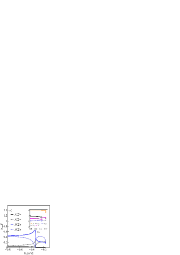
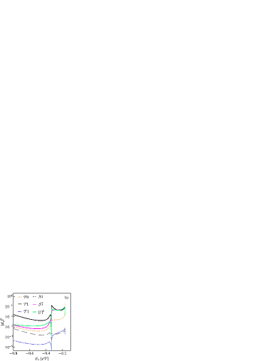
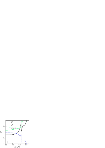
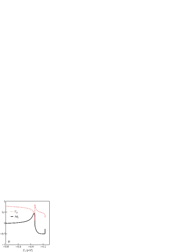
Figure 16: (Color online) Expectation values of slave boson operators, polarizations and expectation values of orbital pseudospin and magnetic moment of Co impurity at $h_{1}$ position of 4ZGNR a) triple occupation slave boson operators $|t_{m\sigma}|^{2}$ b) double and full occupation SB operators $|d_{{\cal{T}}0}|^{2}$, $|d_{{\cal{T}}1}|^{2}$, $|d_{{\cal{T}}\overline{1}}|^{2}$, $|d_{{\cal{S}}1}|^{2}$, $|d_{{\cal{S}}\overline{1}}|^{2}$, $|d_{{\cal{S}}0}|^{2}=|d_{{\cal{T}}0}|^{2}$ and $|f|^{2}$ c) local spin polarization of the nanoribbon around $h_{1}$ (${\cal{P}}_{{\cal{S}}_{{\cal{ZGNR}}}}=\sum_{i}\frac{\varrho_{i+}({\cal{E}}_{\cal{F}})-\varrho_{i-}({\cal{E}}_{\cal{F}})}{\varrho_{i+}({\cal{E}}_{\cal{F}})+\varrho_{i-}({\cal{E}}_{\cal{F}})}$, where $\varrho_{i\sigma}$ denotes local ZGNR density of states at the n. n. carbon sites around hollow position), orbital (${\cal{P}}_{{\cal{O}}}$) and spin polarization of Co adatom (${\cal{P}}_{{\cal{S}}}$) d) magnetic moment and orbital pseudospin of Co impurity. Inset of Fig. a presents spin and orbital resolved contributions to the occupancies of Co.

Let us first discuss the $h_{2}$ case, where local nanoribbon environment is unpolarized. Figures 14 present expectation values of slave boson operators, orbital and spin occupations, orbital and spin moments, orbital and spin polarizations, all quantities plotted as a function of chemical potential. To interpret the results it is worth to refer to the energy dependence of the corresponding hybridization functions (Fig. 13). Outside the singularities ($-0.8<{\cal{E}}<-0.4$) , where hybridization function of $yz$ symmetry dominates over $xz$ hybridization, Kondo physics is governed mainly by spin fluctuations in $yz$ sector (${\cal{N}}_{yz}\approx 1$) , orbital $xz$ is almost completely filled (${\cal{N}}_{xz}\approx 2$). We have checked that there are no SBMFA solutions for $xz$ channel when the interorbital fluctuation path is closed (i.e. when the two last terms in (3) are neglected). When interorbital path opens the coupled spin-orbital fluctuations create resonances in both orbital sectors. Very crudely one can visualize these processes as virtual complete filling or emptying of $yz$ orbital by hoppings resulting in fast SU(2) type spin fluctuations in $yz$ channel (broad peak). These fluctuations are however not completely decoupled from $xz$ channel. Orbital $xz$ is much weaker coupled to nanoribbon and hoppings are less frequent. Virtual creation of a hole on $xz$ orbital increases the probability of double occupancy of $yz$ orbital. Temporary the reverse of roles of orbitals is possible. Such orbital fluctuations enable weak effective spin fluctuations in $xz$ sector despite its high occupancy. The average time of such fluctuations is however relatively long, what reflects in an observed narrow $xz$ quasiparticle resonance . The representative density of states of $h_{2}$ impurity in this range (${\cal{E}}_{{\cal{F}}}=-0.8$) is shown in Figure 15.

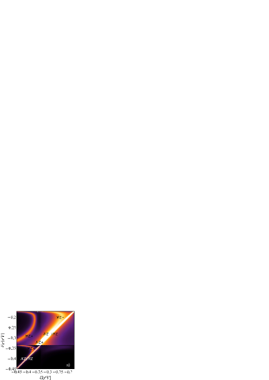
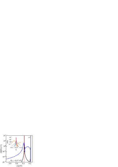
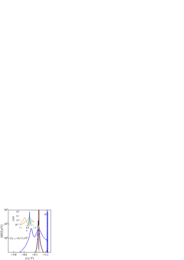
Figure 17: (Color online) a) Density of states map of Co impurity in $h_{1}$ position of 4ZGNR b, c, d) partial orbital densities of states for the selected values of the Fermi levels. Inset are the zoom-views of the spin and orbital resolved DOS.

When ${\cal{E}}_{{\cal{F}}}$ moves closer to singularity ${\cal{VH}}2\nu$, $yz$ hybridization does not change considerably, but in $xz$ sector Van Hove singularity manifests strongly. Close to ${\cal{VH}}2\nu$ the expectation values of slave boson operators $t$ and orbital occupations approach each other in consequence of strong enhancement of $xz$ hybridization, but symmetric SU(4) case is not realized for any energy because this would require the equality of both real and imaginary parts of hybridizations functions. As it is seen in Fig. 15b the resonances in this region for both orbitals (${\cal{E}}=-0.35$ eV) are distinctively different. Interestingly, moving still closer to singularity around (${\cal{E}}=-0.3345$), in an extremely narrow energy range, orbital $xz$ even takes over the dominant role in many-body processes, what reflects in a change of sign of orbital pseudospin. In the region of singularity strong deviations of orbital occupancies from integer values are observed what indicates, that system is driven out from Kondo state into mixed valence state.

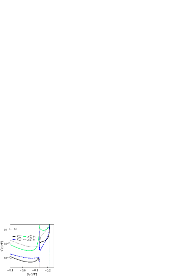
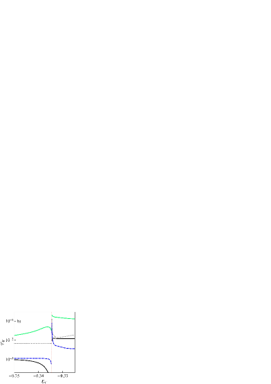
Figure 18: (Color online) Characteristic quasiparticles temperatures $T_{{\cal{K}}}$ for $xz$ and $yz$ channels vs. position of the Fermi level. Fig. b presents details of dependencies close to ${\cal{VH}}2\nu$ singularity.

For chemical potential above ${\cal{VH}}2\nu$ again the dominance of $yz$ orbital is restored and system moves into Kondo state again. One should remember however, that the presented picture in vicinity of singularity should be treated with caution, only as a crude visualization of tendencies. Around singularity the system is pushed into non-Fermi liquid regime due to the observed divergences of self energies, and in principle for a discussion of this range summation of higher order corrections to MFA is indispensable Irkhin ; Irkhin2 . When ${\cal{E}}_{{\cal{F}}}$ moves closer to the edge and both real and imaginary parts of hybridization are strongly enhanced for both symmetries broadening of many-body resonances results and delta like structures are observed at the band edges, which extend into the gap for ${\cal{E}}_{{\cal{F}}}$ moving very close to the edge (Fig. 15c, d). They reflect the new poles of impurity Green’s function and these structures are essential in order to satisfy the sum rules. Of interest are also the dips occurring for energies where singularities occur. They emerge due to an interplay of correlations effect and singular substrate electron density of states. When Fermi level crosses the singularity the dip sits at the the Fermi level, but singularities also reflect in spectral function when chemical potential is not in close proximity to VHS (Fig. 15).

Let us now turn to $h_{1}$ case. The spin polarization of nanoribbon breaks the spin degeneracy. The number of independent slave boson operators increases and the many body resonances become spin dependent. Again of special interest are the regions around singularities of DOS. In addition to the earlier described effects, also new phenomena associated with polarization are observed. The sharp change of local nanoribbon spin polarization in the vicinity of ${\cal{VH}}2\nu$ reveals in a drastic, but opposite change of impurity polarization and suppression of screening processes of Co magnetic moment. Singularity most strongly reflects in the abrupt increase of spin distinction in $yz$ orbital channel what is a consequence of clearly exhibited singularity in the corresponding hybridization function for one spin direction and only very weak trace of it for the opposite spin. Remarkable is the resulting jump and change of sign of magnetic moment and fall and next jump of orbital pseudospin when ${\cal{E}}_{{\cal{F}}}$ crosses singularity. All the anomalies are the consequence of dramatically enhanced imaginary part of hybridization and a jump from negative to positive values of the real part of hybridization. The dramatic changes of spin or orbital characteristics when Fermi level crosses the singularities is of potential interest for spintronics (orbitronics) since these changes can be induced by gate voltage.

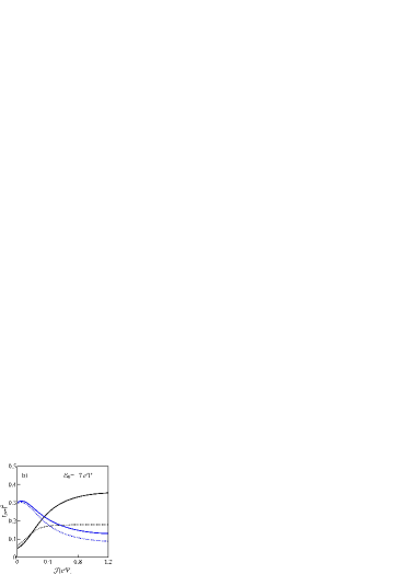
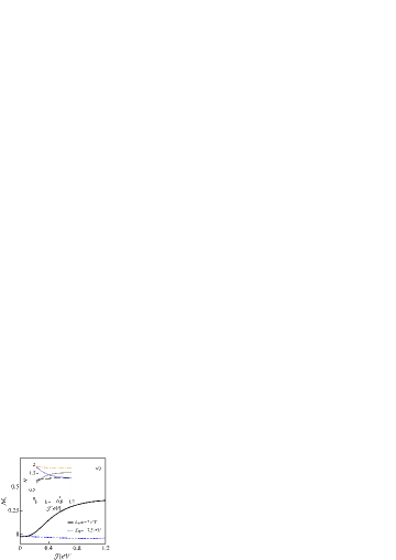
Figure 19: (Color online) Illustration of characteristics of the Kondo state on the value of exchange parameter a, b) slave boson expectation values $|t_{m\sigma}|^{2}$ for ${\cal{N}}\approx 3$ ($\varepsilon_{0}=-7.5$ eV) and ${\cal{N}}\approx 2.7$ ($\varepsilon_{0}=-7$ eV) occupancies (${\cal{E}}_{{\cal{F}}}=-0.8$). c) Magnetic moments of Co impurity. Inset shows orbital occupancies: for $\varepsilon_{0}=-7.5$ dashed line (${\cal{N}}_{yz}$) and dashed-dotted line (${\cal{N}}_{xz}$), $\varepsilon_{0}=-7$ solid line (${\cal{N}}_{yz}$) and dotted line (${\cal{N}}_{xz}$). d) Relative Kondo temperature.

Fig. 17a illustrates the evolution of density of states with the shift of the Fermi level. We have also marked the lines of maxima of DOS. The clearly seen horizontal (${\cal{E}}_{{\cal{F}}}=-0.3348eV$) and vertical (${\cal{E}}=-0.3348eV$) straight lines of reduced intensity reflect the position of ${\cal{VH}}2\nu$ singularity. The representative spin and orbital resolved densities of states, which correspond to the selected horizontal cross sections (${\cal{E}}_{{\cal{F}}}=const$) of the map (Fig. 17a) are displayed in Figure 17b, c, d. Since in the considered energy range $yz$ hybridization is stronger than for $xz$ symmetry the corresponding many body $yz$ resonances are in general broader. Although spin distinction in $xz$ hybridization is remarkable (Fig. 12) it does not reflect in clear distinction of corresponding many-body peaks (Fig. 17). This observation is in accordance with our earlier interpretation of $xz$ resonance as a repercussion of spin fluctuations in $yz$ shell transferred to $xz$ by orbital fluctuations. In contrast to the $h_{2}$ case, for $h_{1}$ position ${\cal{VH}}2\nu$ singularity plays an important role for $yz$ symmetry, especially for majority spins. The peak splitting of $yz$ resonance is a combined effect of spin dependence and singularity induced dips in the corresponding densities of states. Fig. 18 presents Kondo temperatures for $h_{1}$ and $h_{2}$ positions. We define $T_{{\cal{K}}}$ through widths and position of quasiparticle resonance Hewson . $T_{{\cal{K}}m}=(1/2)\sum_{\sigma}\sqrt{\widetilde{\Delta}^{2}_{m\sigma}+\widetilde{{\cal{E}}}^{2}_{m\sigma}}$, where $\widetilde{{\cal{E}}}_{m\sigma}$ is the distance between Fermi energy and quasiparticle resonance and $\widetilde{\Delta}_{m\sigma}$ is the width at half maximum. Since the characteristic quasiparticles energies are distinctively different for both orbital channels we show the corresponding characteristic temperatures separately. The estimated characteristic temperatures are of order of $20$ K and $200$ K for $xz$ and $yz$ channels respectively, and they are strongly enhanced or suppressed in the region of singularity depending on which side the chemical potential approaches the singularity. This tendency reflects the opposite shift of effective orbital energies on both sides caused by real parts of self energy which are discontinuous and change sign in the singularity point. Fig. 19 illustrates an impact of Hund’s coupling on Kondo physics. We show two examples ${\cal{N}}\approx 3$ and ${\cal{N}}\approx 2.7$. Insight on the slave boson dependencies and orbital occupancies highlights the stronger impact of Hund’s coupling for ${\cal{N}}\approx 2.7$. In this case a remarkable weakening of Kondo screening is observed for high values of exchange coupling (increase of magnetic moment). In general one can expect that an increase of magnetic correlations with the increase of exchange coupling should result, as a consequence of competitiveness of different correlations, in a decrease of Kondo temperature. The spin and orbital degrees of freedom fluctuate less freely in this case. This general tendency is really observed in most presented cases. For reduced occupancy however, ${\cal{N}}\approx 2.7$ characteristic temperature $T^{yz}_{{\cal{K}}}$ changes nonmonotonically, what reflects change of partial occupancy form slightly below half filling to values above. For ${\cal{N}}_{yz}=1$ a maximum of Kondo temperature is observed.

III.4 Charge fluctuation effects - NCA and EOM approaches

The SBMFA results get less good with increasing temperature due to fluctuations. Some account of fluctuations is achieved by systematic corrections to MFA approach using e.g. hybridization expansion or applying the equation of motion method. In this section we briefly analyze the role of charge fluctuations in the considered many-body processes. For transparency of considerations we discuss only the case when the chemical potential is located not to close to any VH singularity. We limit to the lowest-order in hybridization self-consistent approximation NCA and EOM with Lacroix’s decoupling approximation Lacroix . These methods apply for higher temperatures, but they give reliable results also down to a fraction of $T_{\cal{K}}$ Bickers ; Hewson ; Kashcheheyevs . They fail however for $T\ll T_{\cal{K}}$, but in this range in turn SBMFA is valid.

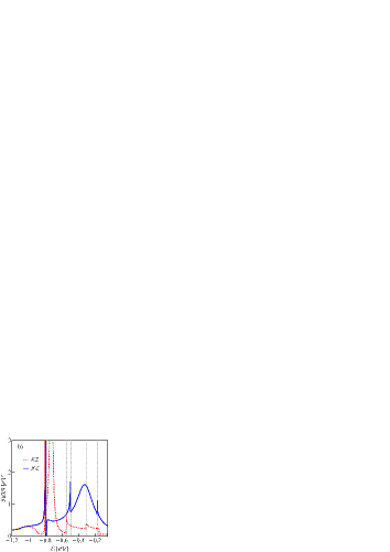
Figure 20: (Color online) Comparison of $xz$ (dotted line) and $yz$ (solid line) contributions to the DOS of Co adatom in $h_{1}$ position of 4ZGNR (${\cal{E}}_{{\cal{F}}}=-0.8$) (NCA). The vertical broken lines on Fig. a determine the positions of bare Coulomb peaks and on Fig. b the positions of singularities in the interacting self energies.

Despite the low temperature deficiencies the use of these impurity solvers allow us to get a crude insight into the full spectrum of the one particle Green’s functions and not just the quasi-particle contribution. In the present work we apply the NCA method for finite ${\cal{U}}$ Pruschke ; Grewe ; Haule ; Gerace . In NCA one takes into account only diagrams without noncrossing of substrate electron lines, what corresponds to simple hopping processes where electron or hole hops into the adatom at some time and then out at a later time. This leads to a set of NCA integral equations for the fixed occupation self energies:

$$\Sigma^{(0)}(z)=\sum_{m\sigma}\int\frac{d\varepsilon}{\pi}\Delta_{m\sigma}(\varepsilon)f(\varepsilon){\cal{G}}^{(1)}_{m\sigma}(z+\varepsilon)$$

$$\Sigma^{(1)}_{m\sigma}(z)=\int\frac{d\varepsilon}{\pi}[\Delta_{m\sigma}(\varepsilon)f(-\varepsilon){\cal{G}}^{(0)}(z-\varepsilon)+\Delta_{m\overline{\sigma}}(\varepsilon)f(\varepsilon){\cal{G}}^{(2)}_{m\sigma m\overline{\sigma}}(z+\varepsilon)$$

$$+\sum_{\sigma^{\prime}}\Delta_{\overline{m}\sigma^{\prime}}(\varepsilon)f(\varepsilon){\cal{G}}^{(2)}_{m\sigma\overline{m}\sigma^{\prime}}(z+\varepsilon)]$$

$$\Sigma^{(2)}_{m\sigma m^{\prime}\sigma^{\prime}}(z)=\int\frac{d\varepsilon}{\pi}[\Delta_{m\sigma}(\varepsilon)f(-\varepsilon){\cal{G}}^{(1)}_{m^{\prime}\sigma^{\prime}}(z-\varepsilon)+\Delta_{m^{\prime}\sigma^{\prime}}(\varepsilon)f(-\varepsilon){\cal{G}}^{(1)}_{m\sigma}(z-\varepsilon)$$

$$+\left\{\begin{array}[]{ll}\Delta_{m^{\prime}\overline{\sigma^{\prime}}}(\varepsilon)f(\varepsilon){\cal{G}}^{(3)}_{m\sigma}(z+\varepsilon)+\Delta_{m\overline{\sigma}}(\varepsilon)f(\varepsilon){\cal{G}}^{(3)}_{m^{\prime}\sigma^{\prime}}(z+\varepsilon),&m\neq m^{\prime}\\ \sum_{\sigma}\Delta_{\overline{m}\sigma}(\varepsilon)f(\varepsilon){\cal{G}}^{(3)}_{\overline{m}\sigma}(z+\varepsilon),&m=m^{\prime}\end{array}\right.]$$ (10)

$$\Sigma^{(3)}_{m\sigma}(z)=\int\frac{d\varepsilon}{\pi}[\Delta_{m\sigma}(\varepsilon)f(-\varepsilon){\cal{G}}^{(2)}_{\overline{m}\sigma\overline{m}\overline{\sigma}}(z-\varepsilon)+\sum_{\sigma^{\prime}}\Delta_{\overline{m}\overline{\sigma^{\prime}}}(\varepsilon)f(-\varepsilon){\cal{G}}^{(2)}_{m\sigma\overline{m}\sigma^{\prime}}(z-\varepsilon)$$

$$+\Delta_{m\overline{\sigma}}(\varepsilon)f(\varepsilon){\cal{G}}^{(4)}(z+\varepsilon)]$$

$$\Sigma^{(4)}=\sum_{m\sigma}\int\frac{d\varepsilon}{\pi}\Delta_{m\overline{\sigma}}(\varepsilon)f(-\varepsilon){\cal{G}}^{(3)}_{m\sigma}(z-\varepsilon),$$ (11)

where ${\cal{G}}^{(p)}_{m\sigma}(z)=[z-{\cal{E}}_{(p)}-\Sigma^{(p)}_{m\sigma}(z)]^{-1}$ ($p=1,3$ with energies ${\cal{E}}_{(1)}=\varepsilon_{0}$ and ${\cal{E}}_{(3)}=3\varepsilon_{0}+3{\cal{U}}$) and ${\cal{G}}^{(2)}_{m\sigma m\overline{\sigma}}(z)=[z-{\cal{E}}_{2}-\Sigma^{(2)}_{m\sigma m\overline{\sigma}}(z)]^{-1}$ (${\cal{E}}_{2}=2\varepsilon_{0}+{\cal{U}}$), ${\cal{G}}^{(4)}(z)=[z-{\cal{E}}_{4}-\Sigma^{(4)}(z)]^{-1}$ (where ${\cal{E}}_{4}=4\varepsilon_{0}+6{\cal{U}}$) are pseudoparticle fermion and boson propagators. Fermion resolvents correspond to odd occupancies of adatom and boson to even. $f(\varepsilon)$ is the Fermi distribution function and $\Delta_{m\sigma}(\varepsilon)=-Im[\Sigma_{m\sigma}(\varepsilon)]$. The retarded local Green’s functions may be evaluated by analytic continuation from the corresponding imaginary time propagator and can be expressed as convolution of pseudoparticle Green’s functions:

$${\cal{G}}_{m\sigma}(i\omega)=(1/{\cal{Z}})\oint_{{\cal{C}}}\frac{dz}{2\pi i}e^{-z/(k_{B}T)}[{\cal{G}}^{(0)}(z){\cal{G}}^{(1)}_{m\sigma}(z+i\omega)+{\cal{G}}^{(1)}_{m\overline{\sigma}}(z){\cal{G}}^{(2)}_{m\sigma m\overline{\sigma}}(z+i\omega)$$

$$+\sum_{\sigma^{\prime}}{\cal{G}}^{(1)}_{\overline{m}\sigma^{\prime}}(z){\cal{G}}^{(2)}_{m\sigma\overline{m}\sigma^{\prime}}(z+i\omega)+\sum_{\sigma^{\prime}}{\cal{G}}^{(2)}_{m\overline{\sigma}\overline{m}\sigma^{\prime}}(z){\cal{G}}^{(3)}_{\overline{m}\sigma^{\prime}}(z+i\omega)$$

$$+{\cal{G}}^{(2)}_{\overline{m}\sigma\overline{m}\overline{\sigma}}(z){\cal{G}}^{(3)}_{m\sigma}(z+i\omega)+{\cal{G}}^{(3)}_{m\overline{\sigma}}(z){\cal{G}}^{(4)}(z+i\omega)],$$ (12)

where ${\cal{Z}}$ is the impurity partition function, i.e.,

$${\cal{Z}}=\oint_{{\cal{C}}}\frac{dz}{2\pi i}e^{-z/(k_{B}T)}[{\cal{G}}^{(0)}(z)+\sum_{m\sigma}{\cal{G}}^{(1)}_{m\sigma}(z)+\sum_{m\sigma m^{\prime}\sigma^{\prime}}{\cal{G}}^{(2)}_{m\sigma m^{\prime}\sigma^{\prime}}(z)$$

$$+\sum_{m\sigma}{\cal{G}}^{(3)}_{m\sigma}(z)+{\cal{G}}^{4}(z)]$$ (13)

It is known that noncrossing approximations encounter difficulties in the case of broken symmetry, it can produce at low temperatures spurious peaks in DOS Wingreen , but we have not observed such artifacts for the examined case. The complementary method we use EOM, consists in differentiating the Green’s functions with respect to time which generates the hierarchy of equations with higher order GFs (11). For the discussed ${\cal{N}}=3$ case apart from single and two electron also three and four particle Green’s functions play the role. In order to truncate the series of EOM equations, we use the generalized procedure proposed by Lacroix Lacroix which approximates the GFs involving two conduction electron operators by single particle correlations and the corresponding Green’s function of lower order:

$$\langle\langle c^{+}_{kn\overline{\sigma}}c_{qn\sigma}d_{m^{\prime}\overline{\sigma}}{\cal{O}};d^{+}_{m\sigma}\rangle\rangle\simeq-\langle c^{+}_{kn\overline{\sigma}}d_{m^{\prime}\overline{\sigma}}\rangle\langle\langle c_{qn\sigma}{\cal{O}};d^{+}_{m\sigma}\rangle\rangle$$

$$\langle\langle c^{+}_{kn\overline{\sigma}}d_{m\sigma}c_{qn\overline{\sigma}}{\cal{O}};d^{+}_{m\sigma}\rangle\rangle\simeq-\langle c^{+}_{kn\overline{\sigma}}c_{qn\overline{\sigma}}\rangle\langle\langle d_{m\sigma}{\cal{O}};d^{+}_{m\sigma}\rangle\rangle$$

$$\langle\langle d^{+}_{m^{\prime}\overline{\sigma}}c_{qn\sigma}c_{kn\overline{\sigma}}{\cal{O}};d^{+}_{m\sigma}\rangle\rangle\simeq-\langle d^{+}_{m^{\prime}\overline{\sigma}}c_{kn\overline{\sigma}}\rangle\langle\langle c_{qn\sigma}{\cal{O}};d^{+}_{m\sigma}\rangle\rangle$$

$$\langle\langle c^{+}_{qn\overline{\sigma}}c_{kn\overline{\sigma}}d_{m\sigma}{\cal{O}};d^{+}_{m\sigma}\rangle\rangle\simeq+\langle c^{+}_{qn\overline{\sigma}}c_{kn\overline{\sigma}}\rangle\langle\langle d_{m\sigma}{\cal{O}};d^{+}_{m\sigma}\rangle\rangle,$$ (14)

where $m^{\prime}=xz(yz)$ and ${\cal{O}}=1,n_{m_{1}\sigma_{1}},n_{m_{1}\sigma_{1}}n_{m_{2}\sigma_{2}}$. The correlations $\langle c^{+}_{kn\sigma}d_{m^{\prime}\sigma}\rangle$ and $\langle c^{+}_{kn\sigma}c_{qn\sigma}\rangle$ occurring in Eq (11) play the leading role in Kondo effect. Upon calculating these averages self-consistently using the spectral theorem and corresponding Green’s functions the EOM set is closed and can be therefore solved. For detailed analysis of EOM hierarchy and decoupling schemes see e.g. Refs.Kashcheheyevs ; Entin .

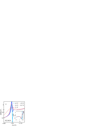
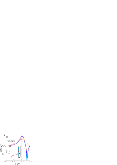
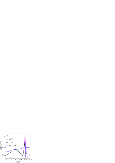
Figure 21: (Color online) Density of states of Co impurity at $h_{1}$ position (${\cal{E}}_{{\cal{F}}}=-0.8$) a, b) temperature evolution of orbital partial densities of states calculated with the use of NCA approximation (Insets are the extended views for $T=0.6$ K and $55.7$ K.) c, d) comparison of NCA DOS with EOM spectra and SBMFA densities of states.

The one particle NCA spectrum is assembled in Fig. 20. For the assumed position of the Fermi level (${\cal{E}}_{{\cal{F}}}=-0.8$) the main contribution comes from convolution of ${\cal{G}}^{(2)}$ and ${\cal{G}}^{(3)}$ functions. In addition to the many-body resonances located around ${\cal{E}}_{\cal{F}}$, also charge fluctuations peaks are visible reflecting fluctuations into fully, doubly, single occupied and empty $\{d_{xz}$, $d_{yz}\}$ shell. Their positions are renormalized and the peaks are broadened as a result of combined effect of hybridization and many body correlations. The Coulomb peaks are only weakly temperature dependent, whereas significant temperature evolution of many-body resonances is observed (Fig. 21a, b). The energy scales of spin-orbital fluctuations and charge fluctuations are not well separated and especially (${\cal{N}}=3$, ${\cal{N}}=4$) Coulomb resonances strongly perturb quasiparticle resonances. The singularities of the nanoribbon spectrum can influence the physics around Fermi level despite the fact that they are not located close to ${\cal{E}}_{{\cal{F}}}$. The observed dips are not direct traces of singularities of hybridization function, they reflect singularities of interacting self energies, which describe repeated conversion of doubly (triple) occupied impurity into single and triple (double and fully) occupied adatom by emitting or absorbing nanoribbon electron. The singularities of interacting self energies however have as source corresponding Van Hove singularities of density of states. Tracing formal generation of singularities via equations (8) one can point out these connections. For example one can identify that singularities at ${\cal{E}}=-0.79$ and ${\cal{E}}=-0.78$ originate from ${\cal{VH}}3\nu$ of hybridization function, these at ${\cal{E}}=-0.55$ and ${\cal{E}}=-0.5$ come from ${\cal{VH}}3c$ singularity and at ${\cal{E}}=-0.31$ and ${\cal{E}}=-0.18$ in turn from ${\cal{VH}}4\nu$ etc. (see Figs. 11b, 20b). The main features of EOM spectrum are similar to NCA results.

Figure 22: (Color online) Partial $xz$ DOS of Co adatom calculated by EOM with realistic (DFT) hybridization function of ZGNR with Lacroix’s decoupling (solid blue line), without dynamical correlations (red dotted line). Broken black curve presents the corresponding DOS calculated with Lacroix’s decoupling, but using energy independent, constant hybridization function.

Charge fluctuation peaks show up more clearly in EOM and the observed impact of charge fluctuation peaks next to the Fermi level on the many-body resonances is stronger than in NCA. Similarly to NCA calculations also in EOM density of states a dip introduced by interacting self-energies, being a reminiscence of singularity of nanoribbon electronic structure is visible. The sharp dips appearing in the presented spectra would certainly be partially smoothed out if finite lifetime effects were take into account similarly to the presented temperature effects (Figs. 20b, c). This remark concerns mainly the impact of singularities on interacting self-energies, because they probe also electrons away from the Fermi level. In some cases, in addition to the dips, peculiarities of electronic structure of the host reflect also in spectral function of impurity as additional peaks (see the peak slightly above the Fermi level in EOM and NCA Co densities of states (Fig. 21). This structure is due to a new pole of the Green’s function - intersection of $\omega-\varepsilon_{0}$ line with the real part of self-energy. Real part of interacting self energy dramatically changes between singularities taking values from a wide range of energy and thus the mentioned intersection is likely in this interval. The occurrence of additional many-body structure is a combined effect of correlations and singularities of nanoribbon DOS. In order to elucidate this point we present in Fig. 22 a comparison of DOS calculated in EOM considering the case of inclusion of dynamical correlations (Lacroix’s decoupling) or neglect of correlations ($\langle c^{\dagger}_{kn\sigma}d_{m\sigma}\rangle=0$) as well as comparing densities of states calculated with hybridization function from DFT with the results, where energy independent hybridization has been assumed. Additional peak above ${\cal{E}}_{\cal{F}}$ is only found when both correlations and full structure of hybridization function is taken into account. The interesting problem of the enriched structure of many-body resonances resulting from peculiarities of electronic structure of the host has been only announced here and we leave a more detailed analysis of this problem as an open question for future work.

IV CONCLUSIONS

For the graphene or its nanostructures, a precise deposition of an atom in a selected position has not yet been implemented, but controlled adatom manipulation for the open surface with the use of atomic force microscopy is within reach of present-day technique Seo ; Gross . It is also possible to probe Kondo effect of magnetic adatoms on surfaces by scanning tunneling spectroscopy Madhavan ; Manoharan ; Mattos . We have addressed in the present study potentially important problem for spintronic applications, the issue of geometrical and electric control of magnetic properties of Kondo impurity on ultranarrow zigzag graphene nanoribbon via peculiarities of its electronic structure. Experiments on Kondo physics in graphene nanoribbons are still missing, but we believe the results presented in this paper will stimulate the experimental effort in this direction. The presented scheme of calculations, which is similar to some other slightly different earlier approaches Korytar ; Karolak ; Wehling ; Jacob combines the first principles calculations with the addition of missing correlations by Hubbard type term and next solving the many-body problem by the well known impurity solvers. The basic input quantity for many-body analysis - hybridization function is determined by impurity - matrix hopping amplitudes and local nanoribbon DFT Green’s functions, both quantities achievable from most output files of DFT programs (e.g. in VASP almost directly code from PROCAR file).

We have shown that Kondo effect of Co impurity in graphene nanoribbon is controlled not only by spin but also by the orbital degrees of freedom. Our DFT analysis showed that only two from five $d$ orbitals are responsible for magnetic properties of impurity. For the preferred hollow positions of Co impurity and chemical potential lying in the vicinity of the gap this role is played by $d_{xz}$, $d_{yz}$ orbitals. In nanoribbon the $C_{6v}$ symmetry of pure graphene is broken and $d_{xz}$, and $d_{yz}$ couple differently to nanoribbon matrix. The presence of the edge states in ZGNR introduces local magnetic polarization close to the edge and consequently breaks also impurity spin degeneracy in this region. The electronic structure of ZGNR is rich in Van Hove singularities and this property can be exploited for electric control of magnetic properties. If Fermi level crosses the singularities the drastic changes of hybridization functions result which in turn reflect in strong alternation of many-body resonances, leading in some cases to transition from Kondo like behavior into mixed valence or even resulting in complete destroying of resonances. For symmetry reasons the specific singularity exhibits differently in different spin and orbital channels and therefore not all channels are equally influenced by its presence. Crossing the singularity by Fermi level results in some cases in an interchange of the roles of orbitals or spins leading to reversal of spin or orbital pseudospin. Since the chemical potential can be shifted by gate voltage, this opens a path of electric field control of these properties. The described effects can be probed by STM. Similarly as the above reported drastic changes of Kondo correlations, also strong impact of singularities on coupling between magnetic impurities is expected Lipinski1 . This problem will be discussed in a forthcoming publication. Our present study shows, that the unconventional electronic and magnetic features of zigzag grapehene nanoribbons not only raise new fundamental issues in many-body physics of adatoms, but also that ZGNRs with impurities can be promising objects for potential applications in spintronics.

- (1) K. S. Novoselov, A. K. Geim, S. V. Morozov, D. Jiang, Y. Zhang, S. V. Dubonos, I. V. Grigorieva, and A. A. Firsov, Science 306, 666 (2004).
- (2) A. K. Geim and K. S. Novoselov, Nature Mat. 6, 183 (2007).
- (3) A. H. Castro Neto, F. Guinea, N. M. R. Peres, K. S. Novoselov, and A. K. Geim, Rev. Mod. Phys. 81, 109 (2009).
- (4) S. Das Sarma, S. Adam, E.H. Hwang, and E. Rossi, Rev. Mod. Phys. 83, 407 470 (2011).
- (5) M.I. Katsnelson, Materials Today 10, 20 (2007).
- (6) P. Avouris, Z. H. Chen, and V. Perebeinos, Nat. Nanotechnol. 2, 605 (2007).
- (7) S.Y. Zhou, G.-H. Gweon, A.V. Fedorov, P.N. First, W.A. der Heer, D.-H. Lee, F. Guinea, A.H. Castro Neto, A. Lanzara, Nature Mat. 6, 770 (2007).
- (8) K. Wakabayashi, K. Sasaki, T. Nakanishi, T. Enoki, Sci. Tech. Adv. Mat. 11, 054504 (2010).
- (9) J. J. Palacios , J. F. Rossier , L. Brey and H. A. Fertig, Semicond. Sci. Technology 25, 033003 (2010).
- (10) L. Pisani, J.A. Chan, B. Montanari, N.M. Harrison, Phys. Rev. B 75, 064418 (2007).
- (11) L. Yang, C.H. Park, Y.-W. Son, M.L. Cohen, and S.G. Louie, Phys. Rev. Lett. 99, 186801 (2007).
- (12) H. Hiura, Appl. Surf. Sci. 222, 374 (2004).
- (13) K. S. Novoselov, A. K. Geim, S. V. Morozov, D. Jiang, M. I. Katsnelson, I. V. Grigorieva, S. V. Dubonos and A. A. Firsov, Nature 438, 197 (2005).
- (14) Y. Zhang, Y. W. Tan, H. L. Stormer, P. Kim, Nature 438, 201 (2005).
- (15) K. Nakada, M. Fujita, G. Dresselhaus, and M. S. Dresselhaus, Phys. Rev. B 54, 17954 (1996).
- (16) B. Özyilmaz, P. Jarillo-Herrero, D. Efetov, D. A. Abanin, L. S. Levitov, and P. Kim, Phys. Rev. Lett. 99, 166804 (2007).
- (17) M. Y. Han, B. Özyilmaz, Y. Zhang, and P. Kim, Phys. Rev. Lett. 98, 206805 (2007).
- (18) M. Fujita, K. Wakabayashi, K. Nakada, and K. Kusakabe, J. Phys. Soc. Jpn. 65, 1920 (1996).
- (19) L. Brey and H. A. Fertig, Phys. Rev. B 73, 235411 (2006).
- (20) Y. Niimi, T. Matsui, H. Kambara, K. Tagami, M. Tsukada, and H. Fukuyama, Phys. Rev. B 73, 085421 (2006).
- (21) Y. Kobayashi, K. I. Fukui, T. Enoki, and K. Kusakabe, Phys. Rev. B 73, 125415 (2006).
- (22) Y.-W. Son, M. L. Cohen, and S. G. Louie, Nature 444, 347 (2006).
- (23) F. Wu, E. Kan, H. Xiang, S.-H. Wei, M.-H. Whangbo, and J. Yang, Appl. Phys. Lett. 94, 223105 (2009).
- (24) C. Tao, L. Jiao, O. V. Yazyev, Y.-C. Chen, J. Feng, X. Zhang, R. B. Capaz, J. M. Tour, A. Zettl, S. G. Louie, H. Dai, and M. F. Crommie, Nature Phys. 7, 616 (2011).
- (25) Y.-W. Son, M. L. Cohen, and S. G. Louie, Phys. Rev. Lett. 97, 216803 (2006).
- (26) J. Kunstmann, C. Özdogan, A. Quandt, H. Fehske, Phys. Rev. B 83, 045414 (2011).
- (27) E. Kan, Z. Li and J. Yang, Nano 03, 433 (2008).
- (28) N. Tombros, C. Jozsa, M. Popinciuc, H. T. Jonkman and B. J. van Wees, Nature 448, 571 (2007).
- (29) Y. Seo and W. Jhe, Rep. Prog. Phys. 71, 016101 (2008).
- (30) L. Gross, F. Mohn, N. Moll, B. Schuler, A. Criado, E . Guitián, D. Penña, A. Gourdon, G. Meyer, Science 337, 1326 (2012).
- (31) E. Kan, H. Xiang, J. L. Yang, and J. G. Hou, J. Chem. Phys. 127, 164706 (2007).
- (32) R.C. Longo, J. Carrete, J. Ferrer, L.J. Gallego, Phys. Rev. B 81, 115418 (2010).
- (33) S. R. Power, V. M. de Menezes, S. B. Fagan, and M. S. Ferreira, Phys. Rev. B 84, 195431 (2011).
- (34) H. Sevinçli, M. Topsakal, E. Durgun, and S. Ciraci, Phys. Rev. B 77, 195434 (2008).
- (35) V. A. Rigo, T. B. Martins, A. J. R. da Silva, A. Fazzio, and R. H. Miwa, Phys. Rev. B 79, 075435 (2009).
- (36) C. Cocchi, D. Prezzi, A. Calzolari, and E. Molinari, J. Chem. Phys. 133, 124703 (2010).
- (37) P. O. Lehtinen, A. S. Foster, Y. Ma, A. V. Krasheninnikov, and R. M. Nieminen, Phys. Rev. Lett. 93, 187202 (2004).
- (38) J. J. Palacios, J. Fernández-Rossier, and L. Brey, Phys. Rev. B 77, 195428 (2008).
- (39) J.-H. Chen, L. Li, W. G. Cullen, E. D. Williams and M. S. Fuhrer, Nature Phys. 7, 535 (2011).
- (40) L. S. Mattos, Ph.D. thesis, Stanford University, 2009; L. S. Mattos, C. R. Moon, P. B. van Stockum, J. C. Randel, H. C. Manoharan, M. W. Sprinkle, C. Berger, W. A. de Heer, K. Sengupta, and A. V. Balatsky, APS March Meeting, Abstract No. T25.009 (American Physical Society, New York, 2009).
- (41) V. Madhavan, W. Chen, T. Jamneala, M. F. Crommie, and N. S. Wingreen, Phys. Rev. B 64, 165412 (2001).
- (42) S.-P. Chao and V. Aji, Phys. Rev. B 83, 165449 (2011).
- (43) B. Uchoa, T. G. Rappoport, and A. H. Castro Neto, Phys. Rev. Lett. 106, 016801 (2011).
- (44) M. Vojta, L. Fritz, and R. Bulla, Europhys. Lett. 90, 27006 (2010).
- (45) Z. G. Zhu, K. H. Ding, and J. Berakdar, Eur. Phys. Lett. 90, 67001 (2010).
- (46) T. O. Wehling, A. V. Balatsky, M. I. Katsnelson, A. I. Lichtenstein, and A. Rosch, Phys. Rev. B 81, 115427 (2010).
- (47) D. Jacob and G. Kotliar, Phys. Rev. B 82, 085423 (2010).
- (48) A.C. Hewson, Kondo Problem to Heavy Fermions, Cambridge University Press, Cambridge, 1993.
- (49) G. Kotliar, and A.E. Ruckenstein, Phys. Rev. Lett. 57, 1362 (1986).
- (50) B. Dong and X. L. Lei, Phys. Rev. B 66, 113310 (2002).
- (51) C. Lacroix, J. Phys. F: Metal Phys. 11, 2389 (1998).
- (52) O. Entin-Wohlman, A. Aharony, and Y. Meir, Phys. Rev. B 71, 035333 (2005).
- (53) V. Kashcheyevs, A. Aharony, and O. Entin-Wohlman, Phys. Rev. B 73, 125338 (2006).
- (54) N. S. Wingreen and Y. Meir: Phys. Rev. B 49, 11040 (1994).
- (55) N. E. Bickers, D. L. Cox, and J. W. Wilkins, Phys. Rev. B 36, 2036 (1987).
- (56) Y. Kuramoto, Z. Phys. B - Condensed Matter 53, 37 (1983).
- (57) Th. Pruschke, N. Grewe, Z. Phys. B - Condens. Matt. 74, 439 (1989).
- (58) N. Grewe, T. Jabben, and S. Schmitt, Eur. Phys. J. B 68, 23 (2009).
- (59) K. Haule, S. Kirchner, J. Kroha, and P. Wölfle, Phys. Rev B 64, 155111 (2001).
- (60) D. Gerace, E. Pavarini, and L. C. Andreani, Phys. Rev. B 65, 155331 (2002).
- (61) P. Hohenberg and W. Kohn, Phys. Rev. 136, B864 (1964).
- (62) J. P. Perdew, K. Burke, and M. Ernzerhof, Phys. Rev. Lett. 77, 3865 (1996).
- (63) J. Heyd, G.E. Scuseria and M. Ernzerhof, J. Chem. Phys. 118, 8207 (2003).
- (64) J. Paier, M. Marsman, K. Hummer, G. Kresse, I. C. Gerber, and J. G. Ángyán, J. Chem. Phys. 124, 154709 (2006).
- (65) R. Gillen, J. Robertson, Phys. Status Solidi B 247, 2945 (2010).
- (66) H. Xiao, J. Tahir-Kheli, and W. A. Goddard, J. Phys. Chem. Lett. 2, 212 (2011).
- (67) S. Park, B. Lee, S. H. Jeon, and S. Han, Current Applied Physics 11, S337 (2011).
- (68) V. Barone, O. Hod, J. E. Peralta and G. E. Scuseria, Acc. Chem. Res. 44, 269 (2011).
- (69) E. -J. Kan, Z. Li, J. Yang, and J. G. Hou, Appl. Phys. Lett. 91, 243116 (2007).
- (70) G. Kresse and J. Furthmüller, Phys. Rev. B 54, 11169 (1996).
- (71) P. E. Blöchl, Phys. Rev. B 50, 17953 (1994); G.Kresse and D. Joubert, Phys. Rev. B 59, 1758 (1999).
- (72) T. Ozaki, Phys. Rev. B 67, 155108 (2003); T. Ozaki and H. Kino, ibid. 69, 195113 (2004); J. Chem. Phys. 121, 10879 (2004).
- (73) K. T. Chan, J. B. Neaton, and M. L. Cohen, Phys. Rev. B 77, 235430 (2008).
- (74) A. I. Liechtenstein, V. I. Anisimov, J. Zaanen , Phys. Rev. B52, R5467 (1995).
- (75) E. H. Lieb, Phys. Rev. Lett. 62, 1201 (1989).
- (76) H. Xiang, E. Kan, S. H. Wei, M. H. Whangbo and J. Yang, Nano. Lett. 9, 4025 (2009).
- (77) S. Kümmel and L. Kronik, Rev. Mod. Phys. 80, 3 (2008).
- (78) G. Cantele, Y.S. Lee, D. Ninno and N. Marzari, Nano Lett. 9, 3425 (2009).
- (79) D. Jiang, X.Q. Chen, W. Luo, W.A. Shelton, Chem. Phys. Lett. 483, 120 (2009).
- (80) T.B. Martins, R.H. Miwa, A.J. R. da Silva, A. Fazzio, Phys. Rev. Lett. 98, 196803 (2007).
- (81) L. Sun, P. Wei, J. Wei, S. Sanvito and S. Hou, J. Phys.: Condens. Matter 23, 425301 (2011).
- (82) X.H. Zheng, X.L. Wang, L.F. Huang, H. Hao, J. Lan, and Z. Zeng, Phys. Rev. B 86, 081408(R) (2012).
- (83) T. Pruschke, and R. Bulla, Eur. Phys. J. B 44, 217 (2005).
- (84) A. Makarovski, L. An, J. Liu, and G. Finkelstein, Phys. Rev. B 74, 155431 (2006).
- (85) B. R. Bułka and S. Lipiński, Phys. Rev. B 67, 024404 (2003).
- (86) J. S. Lim, M. S. Choi, M. Y. Choi, R. Lopez, and R. Aguado, Phys. Rev. B 74, 205119 (2006).
- (87) S. Lipiński, D. Krychowski, Phys. Rev. B 81, 115327 (2010).
- (88) P. Trocha, Phys. Rev. B 82, 125323 (2010).
- (89) A. N. Rudenko, F. J. Keil, M. I. Katsnelson, and A. I. Lichtenstein, Phys. Rev. B 86, 075422 (2012).
- (90) A. K. Zhuravlev and V. Yu. Irkhin, Phys. Rev. B 84, 245111 (2011).
- (91) V Yu Irkhin, J. Phys.: Condens. Matter 23, 065602 (2011).
- (92) H. C. Manoharan, C. P. Lutz ans D. M. Eigler, Nature 403, 512 (2000).
- (93) R. Korytar, M. Pruneda, J. Junquera, P. Ordejon and N. Lorente, J. Phys.: Condens. Matter 22, 385601 (2010).
- (94) M. Karolak, T. O. Wehling, F. Lechermann and A. I. Lichtenstein, J. Phys.: Condens. Matter 23, 085601 (2011).
- (95) S. Lipiński and D. Krychowski, Acta Physica Pol. A 121, 1063 (2012).