CLASH-VLT: The mass, velocity-anisotropy, and pseudo-phase-space density profiles of the $z=0.44$ galaxy cluster MACS J1206.2-0847

Abstract

Aims. We constrain the mass, velocity-anisotropy, and pseudo-phase-space density profiles of the $z=0.44$ CLASH cluster MACS~J1206.2-0847, using the projected phase-space distribution of cluster galaxies in combination with gravitational lensing.

Methods. We use an unprecedented data-set of $\simeq 600$ redshifts for cluster members, obtained as part of a VLT/VIMOS large program, to constrain the cluster mass profile over the radial range $\sim$0–5 Mpc (0–2.5 virial radii) using the MAMPOSSt and Caustic methods. We then add external constraints from our previous gravitational lensing analysis. We invert the Jeans equation to obtain the velocity-anisotropy profiles of cluster members. With the mass-density and velocity-anisotropy profiles we then obtain the first determination of a cluster pseudo-phase-space density profile.

Results. The kinematics and lensing determinations of the cluster mass profile are in excellent agreement. This is very well fitted by a NFW model with mass $M_{200}=(1.4\pm 0.2)\times 10^{15}\,M_{\odot}$ and concentration $c_{200}=6\pm 1$, only slightly higher than theoretical expectations. Other mass profile models also provide acceptable fits to our data, of (slightly) lower (Burkert, Hernquist, and Softened Isothermal Sphere) or comparable (Einasto) quality than NFW. The velocity anisotropy profiles of the passive and star-forming cluster members are similar, close to isotropic near the center and increasingly radial outside. Passive cluster members follow extremely well the theoretical expectations for the pseudo-phase-space density profile and the relation between the slope of the mass-density profile and the velocity anisotropy. Star-forming cluster members show marginal deviations from theoretical expectations.

Conclusions. This is the most accurate determination of a cluster mass profile out to a radius of 5 Mpc, and the only determination of the velocity-anisotropy and pseudo-phase-space density profiles of both passive and star-forming galaxies for an individual cluster. These profiles provide constraints on the dynamical history of the cluster and its galaxies. Prospects for extending this analysis to a larger cluster sample are discussed.

1 Introduction

Clusters of galaxies are excellent cosmological natural laboratories. They are the most massive systems in dynamical equilibrium, and are thus extremely sensitive and effective cosmological probes, especially through the study of the cluster mass function (e.g. Kravtsov & Borgani 2012, and references herein). These systems are believed to be dominated by dark matter (DM hereafter, Zwicky 1933), so their internal mass distribution can in principle be used to distinguish between DM and alternative theories of gravity (e.g. Clowe et al. 2006), or to constrain the intrinsic physical properties of DM (e.g. Arabadjis et al. 2002; Markevitch et al. 2004; Katgert et al. 2004; Serra & Domínguez Romero 2011).

According to Cold DM cosmological numerical simulations, the radial mass distribution of DM halos is universal, and their mass density profiles can be characterized by a simple function of the radial distance (NFW model hereafter; Navarro et al. 1996, 1997), at least out to the virial radius, $r_{200}$. The NFW model parameters are the virial radius $r_{200}$, and the scale radius $r_{-2}$, that is the radius where the logarithmic derivative of the mass density profile $\gamma\equiv{\rm d}\ln\rho/{\rm d}\ln r=-2$. Equivalently, the NFW model can be characterized by the related parameters, the virial mass $M_{200}$, and the concentration $c_{200}\equiv r_{200}/r_{-2}$. An even better fit to the density profile of cosmological halos can be obtained using the Einasto (1965) model (Navarro et al. 2004). Observations have confirmed that the universal NFW model provides adequate fit to the mass distribution of clusters (e.g. Carlberg et al. 1997a; Geller et al. 1999; van der Marel et al. 2000; King et al. 2002; Biviano & Girardi 2003; Rines et al. 2003a; Kneib et al. 2003; Katgert et al. 2004; Arnaud et al. 2005; Broadhurst et al. 2005; Umetsu et al. 2011; Oguri et al. 2012; Okabe et al. 2013).

Many studies have attempted to explain the NFW-like shape of the mass density profile of cosmological halos, and why this shape is universal, even if universality is still a debated issue (e.g. Ricotti 2003; Tasitsiomi et al. 2004; Merritt et al. 2006; Ricotti et al. 2007). While some studies have found the shape of halo density profiles to depend on cosmology (e.g. Subramanian et al. 2000; Thomas et al. 2001; Salvador-Solé et al. 2007), others have not (Huss et al. 1999a; Wang & White 2009). A general consensus is growing that the universal NFW-like shape, at least in the central regions, is the result of the initial, fast assembly phase of halos (Huss et al. 1999b; Manrique et al. 2003; Arad et al. 2004; Tasitsiomi et al. 2004; Lu et al. 2006; El-Zant 2008; Wang & White 2009; Lapi & Cavaliere 2011), characterized by dynamical processes such as violent and collective relaxation, and phase and chaotic mixing (Hénon 1964; Lynden-Bell 1967; Merritt 2005; Henriksen 2006, and references therein). The following slower accretion phase may be responsible for the outer slope of the density profile (Tasitsiomi et al. 2004; Lu et al. 2006; Hiotelis 2006). Halos would obtain the same, universal density profile independently of details about their collapse (El-Zant 2008; Wang & White 2009) and subsequent merger histories (Dehnen 2005; Kazantzidis et al. 2006; El-Zant 2008; Wang & White 2009; Salvador-Solé et al. 2012).

It has been argued by Taylor & Navarro (2001) that the NFW-like shape is strictly related to the power-law radial behavior of the pseudo-phase-space density profiles of halos identified in cosmological numerical simulations, $Q(r)\equiv\rho/\sigma^{3}\propto r^{-\alpha}$ with $\alpha=-1.875$. This power-law behavior of $Q(r)$ is obeyed by a variety of self-gravitating collisionless systems in equilibrium, not necessarily formed as the result of hierarchical accretion processes, and this suggests that it is a generic result of the collisionless collapse, probably induced by violent relaxation (Austin et al. 2005; Barnes et al. 2006). A similar power-law behavior is also obtained for $Q_{\rm r}(r)$, where the total velocity dispersion $\sigma$ is replaced with its radial component, $\sigma_{\rm r}$ (Dehnen & McLaughlin 2005).

The power-law behavior may however not hold at all radii (Schmidt et al. 2008; Ludlow et al. 2010) and depending on the virialization state of the system, departure from power-law may start already close to the center, or, for more virialized halos, near the virial radius (Ludlow et al. 2010). In any case, the relation is surprisingly similar to the self-similar solution of Bertschinger (1985) for secondary infall onto a spherical perturbation, even if the reason for this similarity remains unexplained.

Dehnen & McLaughlin (2005) have shown that the shape of the density profiles of cosmological halos follows analytically from the power-law behavior of $Q(r)$ if the system obeys the Jeans equation of dynamical equilibrium (Binney & Tremaine 1987), and if a linear $\gamma$-$\beta$ relation holds, with

$$\beta(r)=1-{\sigma_{\theta}^{2}(r)+\sigma_{\phi}^{2}(r)\over 2\,\sigma_{r}^{2}(r)}=1-{\sigma_{\theta}^{2}(r)\over\sigma_{r}^{2}(r)}$$ (1)

where $\sigma_{\theta},\sigma_{\phi}$ are the two tangential components, and $\sigma_{r}$ the radial component, of the velocity dispersion, and the last equivalence is obtained in the case of spherical symmetry. The existence of such a linear $\gamma$-$\beta$ relation has been found by Hansen & Moore (2006) to hold in a variety of halos extracted from numerical simulations,

$$\beta(r)=-0.15-0.19\,\gamma(r)\ .$$ (2)

The reality of this relation has been questioned by Navarro et al. (2010) and Lemze et al. (2012) and yet some relation does seem to exist between the shape of a halo mass density profile and the orbital properties of the halo constituents (see also An & Evans 2006; Hansen et al. 2006; Iguchi et al. 2006; Hansen et al. 2010; Van Hese et al. 2011). For a NFW-like density profile, the $\gamma$-$\beta$ relation would imply isotropic orbits ($\beta\approx 0$) near the center, and more radially anisotropic orbits ($\beta>0$) outside, as observed in DM halos. The radius where $\beta(r)$ departs from isotropy, $r_{\beta}$, is then naturally related to the characteristic scale length $r_{-2}$ of the DM density profile (Barnes et al. 2005; Bellovary et al. 2008). A relation between $r_{-2}$ and $r_{\beta}$ has indeed been found in numerically simulated halos (Barnes et al. 2007; Mamon et al. 2010).

Like the power-law behavior of $Q(r)$, also the $\gamma$-$\beta$ relation might be related to the halo formation process. Isotropization of orbits may result from fluctuations in the gravitational potential during the fast-accretion phase characterized by major mergers, i.e. a sort of violent or chaotic relaxation (Lu et al. 2006; Lapi & Cavaliere 2011). The subsequent slow, gentle phase of mass accretion is unable to isotropize orbits and as a consequence the external, more recently accreted material would tend to move on more radially elongated orbits. Another process capable of generating isotropic orbits near the center of halos from an initial distribution of radial orbits is the radial orbit instability (ROI hereafter). ROI occurs when particles in precessing elongated loop orbits experience a torque due to a slight asymmetry, that causes them to lose some angular momentum and move towards the system center (see, e.g., Bellovary et al. 2008). ROI continues even after the halo has virialized (Barnes et al. 2007).

So far we have seen that the shapes of the mass density and velocity anisotropy profiles seem to carry information on the formation processes of cosmological halos but not on the cosmological model. The latter might however be constrained by the relation between the two parameters of the mass density profile, $c_{200}$ and $M_{200}$, the so-called concentration-mass relation ($cMr$ hereafter). In fact, the halo concentration is determined by the mass fraction accreted into the cluster during the initial fast phase (Lu et al. 2006) so $c_{200}$ and $M_{200}$ identify to a large extent the formation redshift of a halo (see, e.g., Gao et al. 2008; Giocoli et al. 2012b). Observing the $cMr$ at different redshifts can therefore be used to constrain cosmological models (see, e.g., Huss et al. 1999a; Dolag et al. 2004; Wong & Taylor 2012). For example, it has been found that the $cMr$ has opposite slopes in Cold and Hot DM cosmologies (Wang & White 2009), while in dark-energy-dominated Warm DM models the $cMr$ is not monotonous but characterized by a turnover point at group mass scales (Schneider et al. 2012).

At present there is some tension between the observed $cMr$ (e.g. Łokas et al. 2006b; Rines & Diaferio 2006; Buote et al. 2007; Schmidt & Allen 2007; Biviano 2008; Ettori et al. 2010; Okabe et al. 2010; Oguri et al. 2012; Newman et al. 2012) and that obtained in $\Lambda$CDM cosmological simulations (e.g. Navarro et al. 1997; Bullock et al. 2001; Duffy et al. 2008; Gao et al. 2008; Klypin et al. 2011; Muñoz-Cuartas et al. 2011; Giocoli et al. 2012a; Bhattacharya et al. 2013), particularly at the low mass end (galaxy groups). The use of the $cMr$ for discriminating among different cosmological models is however somewhat hampered by our ignorance of baryon-related physical processes that can change halo concentrations, also as a function of halo mass (e.g. El-Zant et al. 2004; Gnedin et al. 2004; Barkana & Loeb 2010; Del Popolo 2010; Fedeli 2012). Rasia et al. (2013) have shown that the effect of baryons is not enough to reconcile the observed and simulated $cMr$. Efficient radiative cooling and weak feedback are needed to reconcile the observed and simulated $cMr$ on the scale of galaxy groups, but this comes at the price of creating tension with other observables, such as the stellar mass fraction (Duffy et al. 2010).

The above theoretical considerations about the universality, the shape, and the origin of cluster mass profiles need to be tested observationally. Determining cluster mass profiles is however not a simple task. Traditionally, this has been done using cluster galaxies as tracers of the gravitational potential (e.g. Kent & Gunn 1982; The & White 1986; van der Marel et al. 2000; Biviano & Girardi 2003; Biviano 2000, and references therein) – this technique has allowed the first discovery of dark matter (Zwicky 1933). The intra-cluster gas has been used as tracer of the gravitational potential since the advent of X-ray astronomy (e.g. Mitchell et al. 1977; Forman & Jones 1982; Fabricant et al. 1986; Briel et al. 1992; Ettori et al. 2002). Cluster masses and mass profiles can also be measured using the Sunyaev-Zeldovich (Sunyaev & Zeldovich 1970) effect (e.g. Pointecouteau et al. 1999; Grego et al. 2000; LaRoque et al. 2003; Muchovej et al. 2007), but perhaps the most direct way is by exploiting the gravitational distortion effects of the cluster potential on the apparent shapes of background galaxies (e.g. Wambsganss et al. 1989; Mellier et al. 1993; Squires et al. 1996; Sand et al. 2002; Dahle et al. 2003; Zitrin et al. 2011) as first suggested by Zwicky (1937).

Using different methods to determine cluster mass profiles is fundamental since different methods suffer from different systematics. For instance, X-ray determinations of cluster masses tend to be underestimated if bulk gas motions and the complex thermal structure of the Intra-Cluster Medium (ICM) are ignored (Rasia et al. 2004, 2006; Lau et al. 2009; Molnar et al. 2010; Cavaliere et al. 2011). Cluster triaxiality and orientation effects tend to bias the mass profile estimates obtained by gravitational lensing (e.g. Meneghetti et al. 2011; Becker & Kravtsov 2011; Feroz & Hobson 2012) and by cluster galaxy kinematics (Cen 1997; Biviano et al. 2006). Comparing different mass profile determinations can therefore help assessing the contribution of non-thermal pressure to the ICM and the elongation along the line-of-sight (e.g. Morandi & Limousin 2012; Sereno et al. 2012). If systematics are well under control, the comparison of independent determinations of cluster mass profiles from gravitational lensing and the kinematics of cluster members can shed light on the very nature of DM (Faber & Visser 2006; Serra & Domínguez Romero 2011).

While different methods can be used to constrain a cluster mass profile, direct determination of its velocity-anisotropy profile $\beta(r)$ can only be achieved by using cluster galaxies as tracers of the gravitational potential (Kent & Gunn 1982; Kent & Sargent 1983; Millington & Peach 1986; Sharples et al. 1988; Natarajan & Kneib 1996; Biviano et al. 1997; Carlberg et al. 1997b; Adami et al. 1998a; Mahdavi et al. 1999; Łokas & Mamon 2003; Biviano & Katgert 2004; Mahdavi & Geller 2004; Benatov et al. 2006; Łokas et al. 2006b; Hwang & Lee 2008; Adami et al. 2009; Biviano & Poggianti 2009; Lemze et al. 2009; Wojtak & Łokas 2010).

In this paper we present a new determination of the mass and velocity anisotropy profiles of a massive, X-ray selected cluster at redshift $z=0.44$, largely based on spectroscopic data collected at ESO VLT. These data have been collected within the ESO Large Programme 186.A-0798 “Dark Matter Mass Distributions of Hubble Treasury Clusters and the Foundations of $\Lambda$CDM Structure Formation Models” (P.I. Piero Rosati). This is an ongoing spectroscopic follow-up of a subset of 14 clusters from the “Cluster Lensing And Supernova survey with Hubble” (CLASH, Postman et al. 2012). The CLASH-VLT Large Programme is aimed at obtaining redshift measurements for 400–600 cluster members and 10–20 lensed multiple images in each cluster field. We combine our cluster mass profile determination based on spectroscopic data for member galaxies, with independent mass profile determinations obtained from the strong and weak gravitational lensing analyses of, respectively, Zitrin et al. (2012) and Umetsu et al. (2012, U12 hereafter). The combined power of the excellent imaging and spectroscopic data allows us to determine the mass profile for a single cluster to an unprecedented accuracy and free of systematics over the radial range $\sim$0–5 Mpc (corresponding to 0–2.5 virial radii). The cluster mass profile so obtained is then used to determine the velocity anisotropy profiles, $\beta(r)$ of both the passive and star-forming cluster galaxy populations, for the first time for an individual cluster, thanks to the large sample of spectroscopic redshifts. This is the highest-redshift determination of $\beta(r)$ for an individual cluster so far. The mass profile and $\beta(r)$ determinations are then used to determine (for the first time ever for a real galaxy cluster) the pseudo-phase-space density profiles $Q(r)$ and $Q_{\rm r}(r)$, and the $\gamma$-$\beta$ relation.

The paper is organized as follows. In Section 2 we describe the data sample, and the identification of cluster members. We determine the cluster mass profile in Section 3 and compare our results to theoretical expectations for the $cMr$. We determine the cluster velocity anisotropy profile in Section 4. In Section 5 we test observationally the theoretical $Q(r)$, $Q_{\rm r}(r)$, and $\gamma$-$\beta$ relation. We discuss our results in Section 6 and provide our conclusions in Section 7. In Appendix A we show that our results are robust vs. different choices of the method for cluster members identification. In Appendix B we compare our results for the cluster mass with previous, less accurate results from the literature.

Throughout this paper, we adopt $H_{0}=70$ km s^-1 Mpc^-1, $\Omega_{0}=0.3$, $\Omega_{\Lambda}=0.7$. At the cluster redshift, 1 arcmin corresponds to 0.34 Mpc. Magnitudes are in the AB system.

2 The data sample

The cluster MACS J1206.2-0847 was observed in 2012 as part of the ESO Large Programme 186.A-0798 using VIMOS (Le Fèvre et al. 2003) at the ESO VLT. The VIMOS data were acquired using four separate pointings, each with a different quadrant centered on the cluster core. A total of 12 masks were observed (8 LR-Blue masks and 4 MR masks), and each mask was observed for either 3 or $4\times 15$ minutes, for a total of 10.7 hours exposure time. The LR-Blue masks cover the spectral range 370-670 nm with a resolution R=180, while the MR masks cover the range 480-1000 nm with a resolution R=580.

We used VIPGI (Scodeggio et al. 2005) for the spectroscopic data reduction. We assigned a Quality Flag (QF) to each redshift, which qualitatively indicates the reliability of a redshift measurement. We define four redshift quality classes: “secure” (QF=3), “likely” (QF=2), “insecure” (QF=1), and “based on a single-emission-line” (QF=9). To assess the reliability of these four quality classes we compared pairs of duplicate observations having at least one secure measurement. Thus, we could quantify the reliability of each quality class as follows: redshifts with QF=3 are correct with a probability of $>99.99$%, QF=9 with $\sim 92$% probability, QF=2 with $\sim 75$% probability, and QF=1 with $<40$% probability. We do not consider QF=1 redshifts in this paper.

Additional spectra were taken from Lamareille et al. (2006) (3 objects), Jones et al. (2004) (1), Ebeling et al. (2009) (25), and Daniel Kelson (21 observed with IMACS-GISMO at the Magellan telescope, private communication). Archival data from the programs 169.A-0595 (PI: Hans Böhringer; 5 LR-Blue masks) and 082.A-0922 (PI: Mike Lerchster, 1 LR-Red mask), for 952 spectra in the cluster field were reduced following the same procedure used for our new CLASH-VLT data, using the appropriate calibrations.

The final data-set contains 2749 objects with reliable redshift estimates, of which 2513 have $z>0$, 18% of them obtained in MR mode. Repeated measurements of the same spectra were used to estimate the average error on the radial velocities, 75 (153) km s^-1for the spectra observed with the MR (LR, respectively) grism. The average error is sufficiently small not to affect our dynamical analysis, given the large velocity dispersion of the cluster. Full details on the spectroscopic sample observations and data-reduction will be given in Rosati et al. (in prep.).

Photometric data were derived from Suprime-Cam observations at the prime focus of the Subaru telescope, in five bands ($BVR_{c}I_{c}z^{\prime}$, see U12, ). Full details on the derivation of the photometric catalog used in this paper will be given in Mercurio et al. (in prep.).

2.1 Cluster membership: the spectroscopic sample

Several methods exist to identify cluster members in a spectroscopic data-set (see Wojtak et al. 2007, and references therein). Most of them are based on the location of galaxies in projected phase-space, $R,{\rm v}_{{\rm rf}}$. For the cluster center we choose the position of the Brightest Cluster Galaxy (BCG, $\alpha_{\mathrm{J2000}}=12^{\mathrm{h}}06^{\mathrm{m}}12\aas@@fstack{s}15,\delta_{\mathrm{J2000}}=-8\degr 48\arcmin 3\aas@@fstack{\prime\prime}4$ ). The BCG position practically coincides with the X-ray peak position and the center of mass determined by the gravitational lensing analysis (U12), as all these three positions are within 13 kpc from each other.

Figure 1: Histogram of redshifts in the cluster area. The red, hatched histogram shows the main cluster peak identified by the P+G method.

Here we consider two methods to assign the cluster membership, the method of Fadda et al. (1996), that we call ’P+G’ (Peak+Gap), and the ’Clean’ method of Mamon et al. (2013). The two methods are very different; in particular, unlike the Clean method, the P+G method does not make any assumption about the cluster mass profile. In both methods the main peak in the $z$-distribution is identified. For this, P+G uses an algorithm based on adaptive kernels (Pisani 1993), and Clean uses the weighted gaps in the velocity distribution. After the main peak identification (shown in Fig. 1) P+G considers galaxies in moving, overlapping radial bins to reject those that are separated from the main cluster body by a sufficiently large velocity gap (we choose $\Delta{\rm v}_{{\rm rf}}=800$ km s^-1). The Clean method uses a robust estimate of the cluster line-of-sight velocity dispersion, $\sigma_{\rm{los}}$, to guess the cluster mass using a scaling relation. It then adopts the NFW profile, the theoretical $cMr$ of Macciò et al. (2008), and the velocity anisotropy profile model of Mamon et al. (2010), to predict $\sigma_{\rm{los}}(R)$ and to iteratively reject galaxies with $\mid{\rm v}_{{\rm rf}}\mid>2.7\,\sigma_{\rm{los}}$ at any radius.

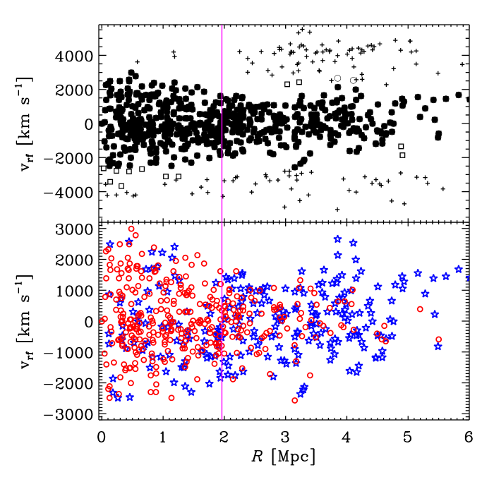
Figure 2: Top panel: Galaxies in the projected phase-space diagram, $R,{\rm v}_{{\rm rf}}$. Black dots represent galaxies identified as cluster members by both the P+G and Clean algorithms. Open circles represent galaxies identified as cluster members by the P+G algorithm only. Squares represent galaxies identified as cluster members by the Clean algorithm only. Crosses represent non-cluster members. Bottom panel: Cluster members selected with the P+G method in the projected phase-space diagram, $R,{\rm v}_{{\rm rf}}$. Red circles represent passive galaxies, blue stars represent SF galaxies. In both panels the vertical (magenta) line indicates $r_{\rm{200,U}}$, i.e. the $r_{200}$ value obtained by scaling the $r_{\Delta}$ estimate of U12 at $\Delta=200$, using their best-fit NFW profile.

In Fig. 2 (top panel) we show the $R,{\rm v}_{{\rm rf}}$ cluster diagram, with the cluster members selected by the two methods. The P+G and Clean method select 592 and 602 cluster membersd, respectively. This is one of the largest spectroscopic sample for members of a single cluster, and the largest at $z>0.4$. There are 590 members in common between the two methods, meaning that only two P+G members are not selected by the Clean method, while 12 Clean members are not selected by the P+G method. Given that the two methods are very different, these differences can be considered quite marginal. Since one of our aims is to determine the cluster mass profile, we prefer to base our analysis on the sample of members defined with the P+G method, because, at variance with the Clean method, it requires no a priori assumptions about the cluster mass profile. In Appendix A we show that our results are little affected if we choose the Clean membership definition instead.

Table 1: Values of the line-of-sight velocity dispersions, $\sigma_{\rm{los}}$, and of the best-fit parameters of the galaxy number density profiles, $n(R)$.

Sample	$\sigma_{\rm{los}}$	$n(R)$
		scale radius $r_{\nu}$		model
	km s-1	[Mpc]
		spec	spec+phot
All	$1087_{-55}^{+53}$	$0.74_{-0.17}^{+0.10}$	$0.63_{-0.09}^{+0.11}$	pNFW
Passive	$1042_{-53}^{+50}$	$0.61_{-0.11}^{+0.15}$	$0.56_{-0.08}^{+0.12}$	pNFW
SF	$1144_{-58}^{+55}$	$0.61_{-0.17}^{+0.20}$	$0.57_{-0.17}^{+0.24}$	King

Using the P+G members, we estimate the cluster mean redshift $\overline{z}=0.43984\pm 0.00015$. The cluster velocity dispersion is given in Table 1 with 1 $\sigma$ errors.

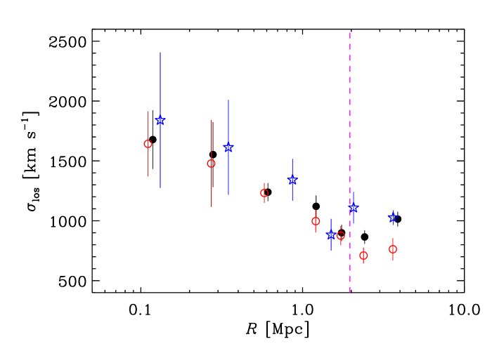
Figure 3: Line-of-sight velocity dispersion profiles of cluster members (using the P+G identification method). Black filled dots: all galaxies; red circles: passive galaxies; blue stars: SF galaxies. 1 $\sigma$ error bars are shown. The vertical magenta dashed line indicates $r_{\rm{200,U}}$.

Since the velocity distribution of late-type/blue/active galaxies in clusters is different from that of early-type/red/passive galaxies and characterized by a larger $\sigma_{\rm{los}}$ (at least in nearby clusters; Tammann 1972; Moss & Dickens 1977; Sodré et al. 1989; Biviano et al. 1992, 1997; Carlberg et al. 1997b; Einasto et al. 2010), it is worth considering a subsample of red/passive galaxies for an estimate of $\sigma_{\rm{los}}$ and, thereby, $r_{200}$. To select a subsample of passive galaxies we use their location in a color-color plot, requiring $(m_{V}-m_{I})\leq-10.47+5.5\,(m_{B}-m_{R})$. This color-color selection separates two subsamples of high-quality spectrum galaxies showing spectroscopic features typical of a passively-evolving stellar population and, separately, of ongoing star-formation (for details see Mercurio et al., in prep.).

The velocity dispersions of passive and star-forming (SF hereafter) galaxies are not significantly different (see Table 1). This is also evident from the distribution of the two samples in the $R,{\rm v}_{{\rm rf}}$ diagram (Fig. 2, bottom panel) and from the $\sigma_{\rm{los}}$ profiles shown in Fig. 3. In nearby clusters there is more difference between the $\sigma_{\rm{los}}$ profiles of the passive and SF galaxy populations, but this difference is known to become less significant in higher-$z$ clusters (Biviano & Poggianti 2009, 2010).

We obtain a first estimate of the cluster $M_{200}$ and $r_{200}$ from the $\sigma_{\rm{los}}$ estimate of the passive cluster members, following the method of Mamon et al. (2013). We assume that (i) the mass is distributed according to the NFW model, (ii) the NFW concentration parameter is obtained iteratively from the mass estimate itself using the $cMr$ of Macciò et al. (2008), and (iii) the velocity anisotropy profile is that of Mamon & Łokas (2005) with a scale radius identical to that of the NFW profile (as found in cluster-mass halos extracted from cosmological numerical simulations, see Mamon et al. 2010, 2013). The procedure is iterative and uses the value of $\sigma_{\rm{los}}$ re-calculated at each iteration on the members within $r_{200}$. We find $M_{200}=1.42\times 10^{15}M_{\odot}$, which corresponds to $r_{200}=1.98$ Mpc. Since $r_{200}\propto\sigma_{\rm{los}}$, the $\sigma_{\rm{los}}$ uncertainty implies a $\simeq 5$% formal fractional uncertainty on the $r_{200}$ estimate, and three times larger on $M_{200}$.

This determination of $r_{200}$ is based on the assumption that the velocity distribution of passive cluster members is unbiased relative to that of DM particles. Numerical simulations suggest that a bias exists, albeit small (e.g. Berlind et al. 2003; Biviano et al. 2006; Munari et al. 2013), so we must take this result with caution. The MAMPOSSt and Caustic methods we will use in the following (see Sects. 3.1 and 3.2) are unaffected by this possible systematics.

Our $\sigma_{\rm{los}}$-based $r_{200}$ value is very close to that obtained by U12 from a gravitational lensing analysis, 1.96 Mpc. We estimate this value using their best-fit NFW $M_{\Delta}$ and $c_{\Delta}$ values converted from their adopted $\Delta=131$ to $\Delta=200$ (we do the same for $c_{\Delta}$, see Table 3). Hereafter we refer to U12’s value of $r_{200}$ as $r_{\rm{200,U}}$.

2.2 Completeness and number density profiles

Our spectroscopic sample is not complete down to a given flux. This can be seen in Fig. 4 where we show the $R_{c}$-band number counts in the cluster virial region ($R\leq 1.96$ Mpc), for all photometric objects, for objects with measured redshifts, and for cluster spectroscopic members (see Sect. 2.1). Note that the target selection in the spectroscopic masks is such to span a wide color range, so that the resulting sample does not have any appreciable bias against galaxies of a given type, which span from early-type to actively star-forming.

The incompleteness of the spectroscopic sample is not relevant for that part of the dynamical analysis which is based on the velocity distribution of cluster members. This distribution can be determined at different radii even with incomplete samples, the only effect of incompleteness being a modulation of the accuracy with which the velocity distribution can be estimated at different radii.

The incompleteness of the spectroscopic sample can instead affect the determination of the cluster projected number density profile, $n(R)$, which converts to the 3D number density profile $\nu(r)$ via the Abel integral equation (Binney & Tremaine 1987). The absolute normalization of the galaxy number density profile $\nu(r)$ is of no concern, however, for our dynamical analysis, since it is only the logarithmic derivative of $\nu(r)$ that enters the Jeans equation (see, e.g., eq. 4 in Katgert et al. 2004). Only if the incompleteness of the sample is not the same at all radii must we be concerned.

Our spectroscopic sample does have a mild radially-dependent incompleteness. This is illustrated in Fig. 5 where we show a spectroscopic-completeness map obtained as the ratio of two adaptive-kernel maps of galaxy number densities, one for all the objects with $z$, and the other for all the photometric objects. In both cases we only consider objects within the magnitude range covered by most of the spectroscopic cluster members, $18\leq m_{R}\leq 23$.

Figure 4: $R_{c}$-band number counts in the cluster virial region (within a radius $R\leq 1.96$ Mpc) for all photometric objects (black histogram), for objects with measured redshifts (hatched blue histogram), and for cluster spectroscopic members (filled red histogram).

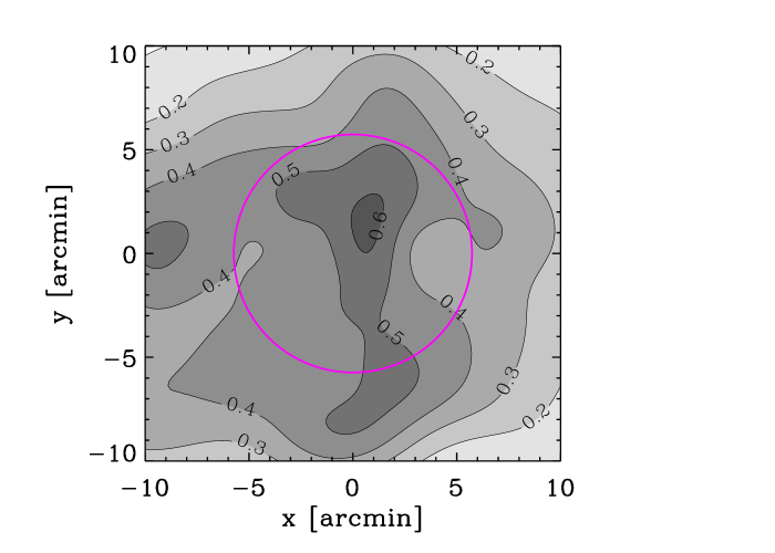
Figure 5: Spectroscopic completeness map. This is the ratio of two adaptive-kernel number density maps, one for all the objects with $z$, and the other for all the photometric objects, both within the magnitude range $18\leq m_{R}\leq 23$. Contours are labeled with the completeness levels, and show that the spectroscopic completeness becomes slightly higher closer to the center. The magenta circle represents the virial region with radius $R\leq r_{\rm{200,U}}$.

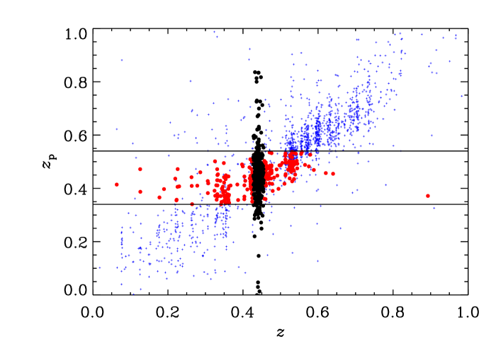
Figure 6: Photometric $z_{\rm p}$ vs. spectroscopic $z$ for the sample of galaxies with $z$ and $18\leq m_{R}\leq 23$ in the cluster field. Spectroscopic cluster members are indicated with black dots, galaxies selected within the $0.34<z_{\rm p}<0.54$ range and within the chosen $m_{R}-m_{I}$ vs. $m_{B}-m_{V}$ color-color cut (see text) are indicated with red (grey) dots. Galaxies outside the photometric and spectroscopic membership selection are indicated with blue crosses.

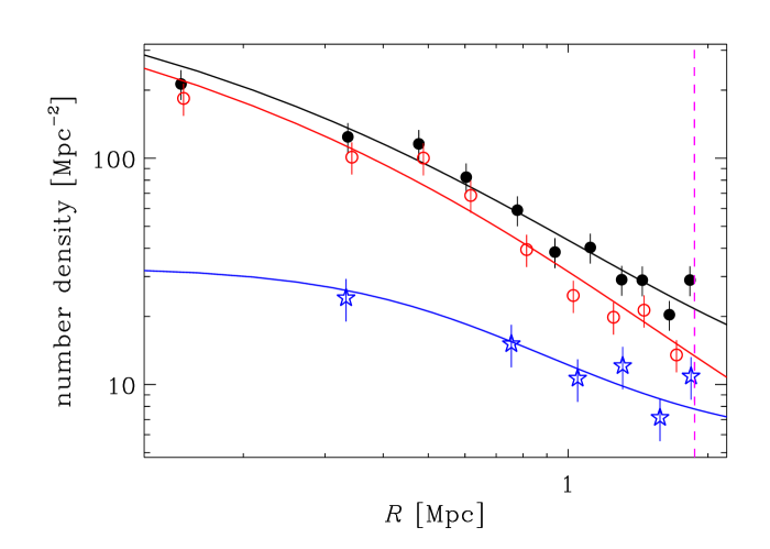
Figure 7: Projected galaxy number density profiles $n(R)$ (symbols with 1 $\sigma$ error bars) and best-fits (solid lines) for the whole cluster population (black filled dots), for the population of passive cluster galaxies (red open dots), and for the population of SF cluster galaxies (blue stars). The best-fit models are pNFW for all and passive members, and the model of King (1962) for the SF members. A constant galaxy density background is added to all models. The vertical magenta dashed line represents $r_{\rm{200,U}}$.

We need to know the radially-dependent completeness correction with an adequate spatial resolution to correctly sample $\nu(r)$ at small radii, but increasing the spatial resolution comes at the price of increasing the Poisson noise of the number counts on which we base our completeness estimates. Given that within $r_{\rm{200,U}}$ the spectroscopic completeness varies by less than $\sim 20$% (Fig. 5) we can, to first approximation, ignore this mild radially-dependent incompleteness. We therefore determine the galaxy $n(R)$ directly from our spectroscopic sample of members within the virial radius and with magnitudes $18\leq m_{R}\leq 23$.

We fit the number density profile of the full sample of cluster members, and, separately, the profiles of the subsamples of passive and SF galaxies (defined in Section 2.1), using a Maximum Likelihood technique, which does not require radial binning of the data (Sarazin 1980). We fit the data with either a projected NFW model (pNFW hereafter; Bartelmann 1996) or with a King model, $n(R)\propto 1/[1+(R/r_{\rm c})^{2}]$ (King 1962; Adami et al. 1998b). The only free parameter in these fits is the scale radius. The results are given in Table 1. The pNFW model provides a better fit than the King model for the samples of all and passive members, while the King model is preferable to the pNFW model for the sample of SF galaxies. All fits are acceptable within the $46$% confidence level, with reduced $\chi^{2}$ of 0.9, 0.6, and 0.3, for the populations of all, passive, and SF galaxies, respectively.

To assess the effect of unaccounted incompleteness bias in our estimates, we now check these results using a nearly complete sample of galaxies. This is the sample of galaxies with available photometric redshifts, $z_{\rm p}$. Note that we only use this photometric sample for the determination of $n(R)$. Our dynamical analysis is entirely based on the spectroscopic sample.

The $z_{\rm p}$ have been obtained by a method based on neural networks. In particular we used the MultiLayer Perceptron (MLP, Rosenblatt 1957) with Quasi Newton learning rule. The MLP architecture is one of the most typical feed-forward neural network model. The term feed-forward is used to identify the basic behavior of such neural models, in which the impulse is propagated always in the same direction, e.g. from neuron input layers towards output layers, through one or more hidden layers (the network brain), by combining sums of weights associated to all neurons (except the input layer). Quasi-Newton Algorithms (QNA) are an optimization of learning rule, in particular they are variable metric methods for finding local maxima and minima of functions (Davidon 1991). The model based on this learning rule and on the MLP network topology is then called MLPQNA (for details on the method see Brescia et al. 2013; Cavuoti et al. 2012).

This method was applied to the whole data-set of $\sim$ 34,000 objects with available and reliable $BVR_{c}I_{c}z^{\prime}$-band magnitudes down to $m_{R}=25.0$, following a procedure of network training and validation based on the subsample of objects with spectroscopic redshifts. We splitted the spectroscopic sample into two subsets, using as the training set 80% of the objects and as the validation set the remaining 20%. In order to ensure a proper coverage of the parameter space we checked that the randomly extracted populations had a spectroscopic distribution compatible with that of the whole spectroscopic sample. Using subsamples of objects with spectroscopically measured redshifts as training and validation sets makes the estimated $z_{{\rm p}}$ insensitive to photometric systematic errors (due to zero points or aperture corrections). In this sense this method is more effective than classical methods based on Spectral Energy Distribution fitting (see Mercurio et al., in prep., for further details on our $z_{{\rm p}}$ estimates).

We must identify cluster members among the galaxies with $z_{{\rm p}}$ and without spectroscopic redshifts to ensure that the number density profile we determine is a fair representation of what we would have obtained using a complete sample of spectroscopic members. We define the cluster membership by requiring $0.34<z_{\rm p}<0.54$ to ensure low contamination by foreground and background galaxies, and yet include most cluster members (see Fig. 6). In the effort to limit field contamination we also apply the following color-color cuts, chosen by inspecting the location of the spectroscopic members in the color-color diagram:

$$-0.09+0.52\,(m_{B}-m_{V})<m_{R}-m_{I}<0.21+0.52\,(m_{B}-m_{V})$$

$$\mbox{for}\;0.20<m_{B}-m_{V}<0.45\ ,$$

$$-0.09+0.52\,(m_{B}-m_{V})<m_{R}-m_{I}<0.36+0.52\,(m_{B}-m_{V})$$

$$\mbox{for}\;0.45\leq m_{B}-m_{V}<0.80\ ,$$

$$0.01+0.52\,(m_{B}-m_{V})<m_{R}-m_{I}<0.36+0.52\,(m_{B}-m_{V})$$

$$\mbox{for}\;0.80\leq m_{B}-m_{V}<1.30.$$

To maximize the number of objects with spectroscopic redshifts we consider the magnitude range $18\leq m_{R}\leq 23$. We then add to this sample the spectroscopic members defined in Sect. 2.1. The combined sample of spectroscopic and photometric members contains 1597 galaxies, of which 54% are photometrically selected.

The purity of the sample of photometrically-selected members can be estimated based on the sample of galaxies with both spectroscopic and photometric redshifts. We define the purity ${\rm P}\equiv N_{pm\cap zm}/N_{pm\cap z}$, where $N_{pm\cap z}$ (respectively, $N_{pm\cap zm}$) is the number of galaxies with $z$ (respectively, the number of spectroscopically confirmed cluster members) which are selected as photometric members. We find ${\rm P}=0.64$. The color-color selection is useful to reduce the contamination, especially by background objects. Had we not used the color-color selection, the purity would have been lowered to 0.50. If we assume the spectroscopic sample of members to have ${\rm P}=1$, the combined sample of photometric and spectroscopic members has ${\rm P}=0.82$.

We fit the number density profiles of this complete sample of (photometrically- and spectroscopically-selected) cluster members, both for the full sample, and for the subsamples of passive and SF galaxies (defined in Section 2.1), within the virial radius, using the same Maximum Likelihood technique already used for the spectroscopic sample. As before we consider either a pNFW or a King model, but this time we add an additional constant background density parameter in both models. The background density parameter is needed because we expect that the photometric membership selection is contaminated by non-cluster members. From the estimate of the purity of the sample, we expect 18% of the selected members to be spurious, and this corresponds to 8 background galaxies Mpc^-2 in our sample of photometrically-selected members, 3/4 of which are SF galaxies. This value is very close to the density of photometrically-selected members in the external cluster regions, $4<R<5$ Mpc, where the field contamination of this sample is likely to be dominant.

Once the background galaxy density parameter is fixed, the only remaining free parameter in the fit is the scale radius. The results of our fits are given in Table 1 and displayed in Fig. 7. The pNFW model provides a better fit than the King model for the samples of all and passive members, while the King model is preferable to the pNFW model for the sample of SF galaxies. All fits are acceptable within the $69$% confidence level, with reduced $\chi^{2}$ of 1.1, 1.2, and 0.8, for the populations of all, passive, and SF galaxies, respectively. These results are very similar to those obtained using the spectroscopically-selected cluster members.

In Sect. 3.1 we will use the $n(R)$ best-fits of the whole cluster population within the MAMPOSSt method. We will consider both results listed in Table 1 to check how much our dynamical results depend on the best-fit solution for the $n(R)$ scale radius.

3 The mass profile

3.1 The MAMPOSSt method

The MAMPOSSt method (Mamon et al. 2013) aims to determine the mass and velocity anisotropy profiles of a cluster in parametrized form, by performing a maximum likelihood fit of the distribution of galaxies in projected phase space. MAMPOSSt does not postulate a shape for the distribution function in terms of energy and angular momentum, and does not suppose Gaussian line-of-sight velocity distributions, but assumes a shape for the 3D velocity distribution (taken to be Gaussian in our analysis). This method has been extensively tested using cluster-mass halos extracted from cosmological simulations. It assumes dynamical equilibrium, hence it should not be applied to data much beyond the virial radius. Following the indications of Mamon et al. (2013) we only consider data within $R\leq r_{200}$. We also exclude the very inner region, within 0.05 Mpc, since it is dominated by the internal dynamics of the BCG, rather than by the overall cluster (see, e.g., Biviano & Salucci 2006). Our MAMPOSSt analysis is therefore based on the sample of 330 cluster members with $0.05\leq R\leq r_{\rm{200,U}}$. Of these, 250 are passive galaxies (see Section 2.1).

The MAMPOSSt method requires parametrized models for the number density, mass, and velocity anisotropy profiles – $\nu(r)$, $M(r)$, $\beta(r)$, but there is no limitation in the possible choice of these models. Since our spectroscopic data-set might suffer from (mild) radial-dependent incompleteness, we prefer not to let MAMPOSSt fit $\nu(r)$ directly; rather, we use the de-projected $n(R)$ best-fit models obtained in Sect. 2.2 (see Table 1). We refer to the scale radius of the number density profile as $r_{\nu}$ in the following.

As for $M(r)$, we consider the following models:

1. the NFW model,

   $$M(r)=M_{200}{\ln(1+r/r_{-2})-r/r_{-2}\,(1+r/r_{-2})^{-1}\over\ln(1+c_{200})-c_{200}/(1+c_{200})}\ ,$$ (3)

2. the Hernquist model (Hernquist 1990),

   $$M(r)={M_{200}\,(r_{\rm H}+r_{200})^{2}\over r_{200}^{2}}{r^{2}\over(r+r_{\rm H})^{2}}\ ,$$ (4)

   where $r_{\rm H}=2\,r_{-2}$,

3. the Einasto model (Einasto 1965; Mamon et al. 2010; Tamm et al. 2012),

   $$M(r)=M_{200}{P[3m,2m\,(r/r_{-2})^{1/m}]\over P[3m,2m\,(r_{200}/r_{-2})^{1/m}]}\,$$ (5)

   where $P(a,x)=\gamma(a,x)/\Gamma(a)$ is the regularized incomplete gamma function, and where we fix $m=5$, a typical value for cluster-size halos extracted from cosmological numerical simulations (Mamon et al. 2010),

4. the Burkert model (Burkert 1995),

   $$M(r)=M_{200}\,\{\ln[1+(r/r_{\rm B})^{2}]+2\ln(1+r/r_{\rm B})$$

   $$-2\arctan(r/r_{\rm B})\}\times\{\ln[1+(r_{200}/r_{\rm B})^{2}]$$

   $$+2\ln(1+r_{200}/r_{\rm B})-2\arctan(r_{200}/r_{\rm B})\}^{-1}\ ,$$ (6)

   where $r_{\rm B}\simeq 2/3\,r_{-2}$,

5. the Softened Isothermal Sphere (SIS model, hereafter; see e.g. Geller et al. 1999)

   $$M(r)=M_{200}{r/r_{\rm I}-\arctan(r/r_{\rm I})\over r_{200}/r_{\rm I}-\arctan(r_{200}/r_{\rm I})}\ ,$$ (7)

   where $r_{\rm I}$ is the core radius.

The NFW and Hernquist mass density profiles are characterized by central logarithmic slopes $\gamma=-1$, while the Burkert and SIS mass density profiles have a central core, $\gamma=0$. Somewhat in between these two extremes, the Einasto profile has not a fixed central slope but one that asymptotically approaches zero near the center, $\gamma=-2\,(r/r_{-2})^{1/m}$. The asymptotic slopes of the NFW, Hernquist, Burkert, and SIS mass density profiles are $\gamma=-3,-4,-3,$ and $-2$, respectively. The NFW and the Einasto models have been shown to successfully describe the mass density profiles of observed clusters (see Section 1). The Hernquist model is well studied (e.g. Baes & Dejonghe 2002) and it has been shown to provide a good fit to the mass profile of galaxy clusters (Rines et al. 2000, 2001, 2003a; Rines & Diaferio 2006). This is also true of the Burkert model (Katgert et al. 2004; Biviano & Salucci 2006), but not of the SIS model (Rines et al. 2003a; Katgert et al. 2004).

As for $\beta(r)$, we consider the following models:

1. ’C’: Constant anisotropy with radius, $\beta=\beta_{C}$;

2. ’T’: from Tiret et al. (2007),

   $$\beta_{\rm T}(r)=\beta_{\infty}\,{r\over r+r_{-2}}\ ,$$ (8)

   isotropic at the center, with anisotropy radius identical to $r_{-2}$, characterized by the anisotropy value at large radii, $\beta_{\infty}$;

3. ’O’: anisotropy of opposite sign at the center and at large radii,

   $$\beta_{\rm O}(r)=\beta_{\infty}\,{r-r_{-2}\over r+r_{-2}}\ ,$$ (9)

The C model is the simplest, and has been frequently used in previous studies (e.g. Merritt 1987; van der Marel et al. 2000; Łokas & Mamon 2003). The T model has been shown by Mamon et al. (2010, 2013) to provide a good fit to the velocity anisotropy profiles of cosmological cluster-mass halos. Here we introduce the O model to account for the possibility of deviation from the general behavior observed in numerically simulated halos – the O model allows for non-isotropic orbits near the cluster center while the T model does not. Isotropic orbits are allowed in all three models. Note that the $r_{-2}$ parameter common to the T and O models is the same parameter that enters the NFW and Einasto $M(r)$ models, and is related to the scale parameters of the Hernquist and Burkert $M(r)$ models. For the SIS model $r_{-2}$ cannot be uniquely defined, hence we can only consider the C $\beta(r)$ model, and not the T and O models.

Table 2: Results of the MAMPOSSt analysis.

Models		$r_{200}$	$r_{\rho}$	Vel.	Lik.	$r_{200}$	$r_{\rho}$	Vel.	Lik.
$M(r)$	$\beta(r)$	[Mpc]	[Mpc]	anis.	ratio	[Mpc]	[Mpc]	anis.	ratio
		$r_{\nu}=0.74$ Mpc				$r_{\nu}=0.63$ Mpc
NFW	C	$1.97_{-0.12}^{+0.06}$	$0.43_{-0.06}^{+0.78}$	$0.4_{-0.1}^{+0.3}$	1.00	$1.99_{-0.09}^{+0.08}$	$0.39_{-0.06}^{+0.65}$	$0.4_{-0.1}^{+0.3}$	1.00
NFW	T	$1.94_{-0.13}^{+0.05}$	$0.36_{-0.02}^{+0.33}$	$0.5_{-0.0}^{+0.4}$	0.87	$1.96_{-0.11}^{+0.05}$	$0.34_{-0.02}^{+0.31}$	$0.5_{-0.0}^{+0.4}$	0.88
NFW	O	$1.94_{-0.10}^{+0.07}$	$0.28_{-0.04}^{+0.15}$	$0.5_{-0.2}^{+0.4}$	0.62	$1.96_{-0.10}^{+0.07}$	$0.27_{-0.04}^{+0.14}$	$0.5_{-0.2}^{+0.4}$	0.65
Hernquist	C	$2.00_{-0.13}^{+0.06}$	$1.13_{-0.13}^{+1.56}$	$0.5_{-0.1}^{+0.3}$	0.89	$2.03_{-0.10}^{+0.07}$	$1.07_{-0.15}^{+1.28}$	$0.5_{-0.1}^{+0.3}$	0.88
Hernquist	T	$1.97_{-0.11}^{+0.05}$	$0.97_{-0.06}^{+0.59}$	$0.6_{-0.0}^{+0.3}$	0.64	$2.00_{-0.10}^{+0.06}$	$0.92_{-0.06}^{+0.56}$	$0.6_{-0.0}^{+0.3}$	0.64
Hernquist	O	$1.98_{-0.09}^{+0.07}$	$0.72_{-0.10}^{+0.28}$	$0.4_{-0.2}^{+0.5}$	0.34	$1.99_{-0.09}^{+0.07}$	$0.70_{-0.09}^{+0.27}$	$0.4_{-0.2}^{+0.5}$	0.35
Einasto	C	$1.98_{-0.14}^{+0.06}$	$0.47_{-0.05}^{+0.88}$	$0.4_{-0.1}^{+0.3}$	1.00	$2.01_{-0.11}^{+0.07}$	$0.42_{-0.05}^{+0.74}$	$0.4_{-0.1}^{+0.3}$	1.00
Einasto	T	$1.95_{-0.13}^{+0.04}$	$0.41_{-0.02}^{+0.34}$	$0.6_{-0.0}^{+0.4}$	0.86	$1.98_{-0.12}^{+0.05}$	$0.39_{-0.02}^{+0.33}$	$0.6_{-0.0}^{+0.4}$	0.87
Einasto	O	$1.95_{-0.10}^{+0.07}$	$0.31_{-0.04}^{+0.16}$	$0.5_{-0.2}^{+0.4}$	0.57	$1.98_{-0.10}^{+0.07}$	$0.30_{-0.04}^{+0.15}$	$0.5_{-0.2}^{+0.4}$	0.59
Burkert	C	$1.99_{-0.09}^{+0.08}$	$0.30_{-0.06}^{+0.33}$	$0.5_{-0.1}^{+0.3}$	0.74	$2.01_{-0.07}^{+0.09}$	$0.27_{-0.05}^{+0.28}$	$0.5_{-0.1}^{+0.3}$	0.73
Burkert	T	$1.96_{-0.10}^{+0.05}$	$0.23_{-0.02}^{+0.16}$	$0.5_{-0.0}^{+0.4}$	0.51	$1.98_{-0.08}^{+0.06}$	$0.22_{-0.02}^{+0.15}$	$0.5_{-0.0}^{+0.4}$	0.52
Burkert	O	$1.96_{-0.09}^{+0.07}$	$0.18_{-0.03}^{+0.07}$	$0.4_{-0.2}^{+0.5}$	0.33	$1.97_{-0.09}^{+0.07}$	$0.17_{-0.03}^{+0.07}$	$0.4_{-0.2}^{+0.5}$	0.34
SIS	C	$1.83_{-0.09}^{+0.10}$	$0.01_{-0.00}^{+0.02}$	$0.5_{-0.2}^{+0.3}$	0.44	$1.88_{-0.10}^{+0.09}$	$0.01_{-0.00}^{+0.03}$	$0.5_{-0.2}^{+0.3}$	0.37

Figure 8: Top panel: Mass profiles as obtained from the MAMPOSSt and Caustic analyses. The MAMPOSSt result is that obtained using the NFW model and the O $\beta(r)$ model, and is represented by a black curve within a grey shaded area (1 $\sigma$ confidence region). The Caustic result is represented by green dash-dotted curves (central value within 1 $\sigma$ confidence region). The black dot and green square represent the locations of the $[r_{200},M_{200}]$ values for the MAMPOSSt and Caustic $M(r)$. Bottom panel: Fractional difference between different mass profiles and the MAMPOSSt best-fit to the NFW $M(r)$ with O $\beta(r)$ model (displayed in the top panel). The MAMPOSSt best-fit O $\beta(r)$ Hernquist, Einasto, and Burkert models are represented by the blue long-dashed, gold triple-dot-dashed, and red short-dashed curves, respectively. The MAMPOSSt best-fit C $\beta(r)$ SIS model is represented by the magenta dotted curve. The Caustic $M(r)$ and 1 $\sigma$ confidence levels are represented by the green dash-dotted curves. The solid line marks the zero and the grey shaded area the 1 $\sigma$ confidence region of the NFW model fit. Symbols represent the location of the $[r_{200},M_{200}/M_{NFW}(r_{200})-1]$ values for the different mass profiles, NFW (filled black dot), Hernquist (blue X), Einasto (gold star), Burkert (red triangle), SIS (magenta inverted triangle), Caustic (green square). The NFW and Burkert values are barely visible in the plot, because they are virtually indistinguishable from the Einasto and Hernquist values. All MAMPOSSt results displayed here are for the $r_{\nu}=0.63$ Mpc value (see Table 2).

Figure 9: Results of the MAMPOSSt analysis using the NFW and O models for $M(r)$ and $\beta(r)$, respectively. The vertical lines and dots indicate the best-fit solutions. The likelihood distributions on each parameter are obtained by marginalizing vs. the other two parameters. Gray-shading in the likelihood distribution plots indicate the 1 $\sigma$ confidence regions. The red, gray-shaded contours are 1 $\sigma$ confidence levels on the two labeled parameters, obtained by marginalizing vs. the third parameter. Note that we show results for $\sigma_{r}/\sigma_{\theta}$ rather than for $\beta$ (see eq. 1).

In total, we run MAMPOSSt with 3 free parameters, i.e. the virial radius $r_{200}$, the scale radius of the total mass distribution $r_{\rho}$ (equal to $r_{-2},r_{\rm H},r_{\rm B}$ or $r_{\rm I}$, depending on the $M(r)$ model), and the anisotropy parameter, $\beta_{C}$ or $\beta_{\infty}$. Note that we do not assume that light traces mass, i.e. we allow the scale radius of the total mass distribution to be different from that of the galaxy distribution, $r_{\rho}\neq r_{\nu}$. The results of the MAMPOSSt analysis are given in Table 2. The best-fits are obtained using the NEWUOA software for unconstrained optimization (Powell 2006). The errors on each of the parameters listed in the table are obtained by a marginalization procedure, i.e. by integrating the probabilities $p(r_{200},r_{\rho},\beta)$ provided by MAMPOSSt, over the remaining two free parameters.

In Table 2 we list two sets of results, one for each of the best-fit values of $r_{\nu}$ found in Sect. 2.2. The results are very similar in the two cases. On average, the values of $r_{200},r_{\rho},$ and $\beta$ or $\beta_{\infty}$ change by 2, 5, and 2 %, respectively. These variations are much smaller than the statistical errors on the parameters, therefore we only consider the set of results obtained for $r_{\nu}=0.63$ Mpc, in the following (this is the value obtained for the complete sample of spectroscopic + photometric cluster members, see Sect. 2.2).

Using the likelihood-ratio test (Meyer 1975) we find that all models are statistically acceptable (likelihood ratios are listed in the last column of Table 2). This is also visible from Fig. 8 where we display the five $M(r)$ corresponding to the best-fit NFW, Hernquist, Einasto, and Burkert models with O $\beta(r)$, and to the best-fit SIS model with $C$ $\beta(r)$. The SIS $M(r)$ is in some tension with the others due to the fact that it is essentially a single power-law, as the value of its core radius $r_{\rm I}$ is constrained by the MAMPOSSt analysis to be very small (see Table  2).

The different models give best-fit values of $r_{200}$ in agreement within their 1 $\sigma$ errors. The rms of all $r_{200}$ values is 0.04, smaller than the error on any individual $r_{200}$ value. This is also true of the $r_{-2}$ parameter (we use the appropriate scaling factors to convert $r_{\rm H}$ and $r_{\rm B}$ to $r_{-2}$), for which the rms is 0.08, and of the anisotropy parameter for which the rms is 0.06.

Since the uncertainties on the values of the parameters are dominated by statistical errors, and not by the systematics induced by the model choice, for simplicity in the rest of this paper we only consider the MAMPOSSt results obtained for one of the considered models. We choose the NFW model for $M(r)$, for the sake of comparing our results to those of U12, and also because it provides slightly higher likelihoods than the Hernquist, Burkert, and SIS mass models (for fixed $\beta(r)$ model) and comparable likelihoods to those of the Einasto model. As for the $\beta(r)$ model, we choose the O model, since it is the one that gives the smallest errors on the $M(r)$ parameters, in the sense of maximizing the figure of merit FoM$\,\equiv(r_{200}\,r_{-2})/(\delta r_{200}\,\delta r_{-2})$, where $\delta r_{200}$ and $\delta r_{-2}$ are the (symmetrized) errors on, respectively, $r_{200}$ and $r_{-2}$. In Fig. 9 we display the results of the MAMPOSSt analysis for the NFW+O models. In Sect. 4 we will show how the best-fit $\beta(r)$ models for the NFW mass model compare with our non-parametric $\beta(r)$ determination from the Jeans inversion (see Fig. 15).

3.2 The Caustic method

The Caustic method (Diaferio & Geller 1997; Diaferio 1999) is based on the identification of density discontinuities in the $R,{\rm v}_{{\rm rf}}$ space. This method does not require the assumption of dynamical equilibrium outside the virial region, hence it makes use of all galaxies, not only of member galaxies, and can provide $M(r)$ also at $r>r_{200}$. Moreover the method does not require to assume a model for $M(r)$. This comes at the price of some simplifying assumptions that can induce systematic errors, as we see below.

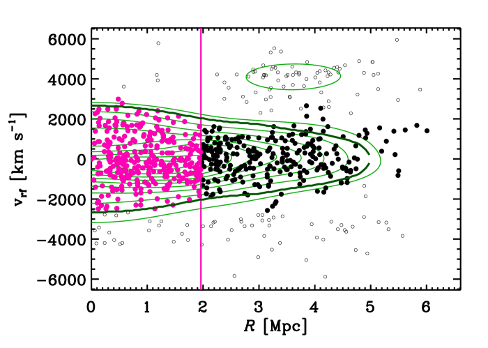
Figure 10: Caustics in the $R,{\rm v}_{{\rm rf}}$ space; the thick-line caustic is the one identified following the prescription of Diaferio (1999). Filled dots identify members selected using the P+G method; the vertical line indicates the location of $r_{\rm{200,U}}$.

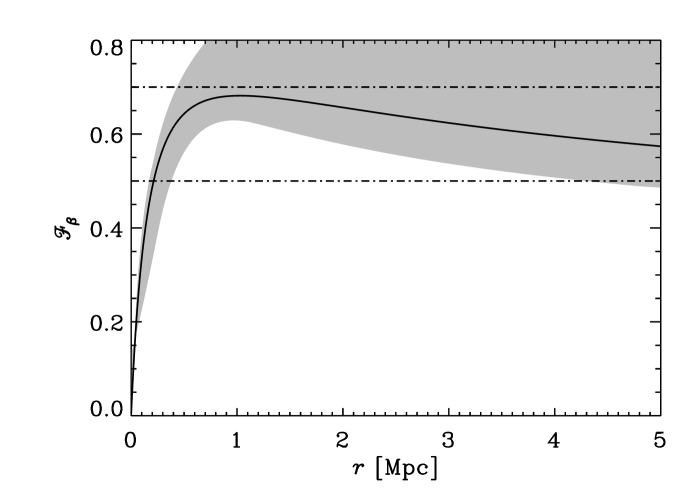
Figure 11: The ${\cal F}_{\beta}$ function obtained by adopting the best-fit $M(r)$ NFW model with an O $\beta(r)$ model, using MAMPOSSt (solid black curve) within 1 $\sigma$ confidence region (hatched gray region). The two horizontal dashed lines indicate two commonly adopted constant values of ${\cal F}_{\beta}$ in the literature.

In Fig. 10 we show the projected phase-space distribution of all galaxies and galaxy iso-number density contours, computed using Gaussian adaptive kernels with an initial ’optimal’ kernel size (as defined in Silverman 1986). Before estimating the density contours, rest-frame velocities and clustercentric distances are scaled in such a way as to have the same dispersion for the scaled radii and scaled velocities. The data-set is mirrored across the $R=0$ axis before the density contours are estimated, to avoid edge-effects problems. To choose the density threshold that defines the contour (the ’caustic’) to use, we follow the prescriptions of Diaferio (1999), which depend on an estimate of the velocity dispersion of cluster members. We use the P+G cluster membership definition (Section 2.1), for consistency with the rest of our dynamical analyses in this paper.

Table 3: Best-fit dynamical parameters for the NFW $M(r)$ model.

Method	Sample	$N_{members}$	$r_{200}$	$r_{-2}$	$M_{200}$	$c_{200}$
		[Mpc]	[Mpc]	[$10^{15}\,M_{\odot}$]
$\sigma_{\rm{los}}$+$r_{\nu}$	$R\leq 1.98$ Mpc (passive only)	261	1.98 $\pm$ 0.10	0.63${}_{-0.09}^{+0.11}$	1.41 $\pm$ 0.21	3.1 $\pm$ 0.5
MAMPOSSt	$0.05\leq R\leq 1.96$ Mpc	330	$1.96_{-0.10}^{+0.07}$	$0.27_{-0.04}^{+0.14}$	$1.37\pm 0.18$	$7.3\pm 2.4$
Caustic	$R\leq 2\times 1.96$ Mpc	527	$2.08_{-0.30}^{+0.09}$	$0.47_{-0.09}^{+0.47}$	$1.63\pm 0.58$	$4.4\pm 3.0$
MAMPOSSt+Caustic			$1.96_{-0.09}^{+0.14}$	$0.35_{-0.09}^{+0.14}$	$1.37\pm 0.24$	$5.6\pm 1.9$
Lensing	U12		$1.96\pm 0.11$	$0.34\pm 0.06$	$1.37\pm 0.23$	$5.8\pm 1.1$

The velocity amplitude of the chosen caustic is related to $M(r)$ via a function of both the gravitational potential and $\beta(r)$, called ${\cal F}_{\beta}$. For simplicity most studies (with the notable exception of Biviano & Girardi 2003) have so far used constant ${\cal F}_{\beta}(r)$, following the initial suggestion of Diaferio & Geller (1997) and Diaferio (1999). With the most recent implementation of the caustic algorithm by Serra et al. (2011), the value of ${\cal F}_{\beta}=0.7$ was adopted. The value ${\cal F}_{\beta}=0.5$ preferred by Diaferio & Geller (1997), Diaferio (1999), and Geller et al. (2013) was appropriate for an earlier implementation of the algorithm that however tended to overestimate the escape velocity by 15–20% on average.

The unknown value of ${\cal F}_{\beta}$ is a major systematic uncertainty in this method. The correct value of ${\cal F}_{\beta}$ to use might be different for different membership definitions, as suggested by the analysis of numerically simulated halos of Serra et al. (2011). For consistency we use for the Caustic method the same membership definition used for the MAMPOSSt analysis (see Sect. 3.1). We can therefore take advantage of our MAMPOSSt-based determinations of $M(r)$ and $\beta(r)$ to determine ${\cal F}_{\beta}$ for the Caustic method.

We adopt the best-fit NFW $M(r)$ + O $\beta(r)$ model (see Table 2) and obtain the ${\cal F}_{\beta}(r)$ shown in Fig. 11. The large uncertainty associated to the $\beta_{\infty}$ parameter of the O model propagates into a large uncertainty on ${\cal F}_{\beta}$. Within the uncertainties ${\cal F}_{\beta}(r)$ is consistent with the value of 0.7 but only at radii $r>0.5$ Mpc. It is instead inconsistent with the value of 0.5 at most radii. Over most of the radial range, ${\cal F}_{\beta}(r)$ is intermediate between these two commonly adopted constant values, but not near the center, where it is smaller. Constant-${\cal F}_{\beta}$ Caustic determinations of $M(r)$ are known to suffer from an overestimate at small radii (Serra et al. 2011); the radial dependence of our adopted ${\cal F}_{\beta}(r)$ is likely to correct for this bias.

The uncertainties in the Caustic $M(r)$ estimate are derived following the prescriptions of Diaferio (1999). According to Serra et al. (2011) these prescriptions lead to estimate 50% confidence levels; we therefore multiply them by 1.4 to have $\sim 1\sigma$ confidence levels.

The Caustic $M(r)$ within its 1 $\sigma$ confidence region is shown in Fig. 8. It is consistent with the $M(r)$ obtained via the MAMPOSSt method. This consistency is at least partly enforced by the fact that we calibrated ${\cal F}_{\beta}(r)$ using the results we obtained with MAMPOSSt.

We obtain the mass density profile $\rho(r)$ from numerical differentiation of the Caustic $M(r)$, and then fit the NFW model, limiting the fit to radii below twice $r_{\rm{200,U}}$ (we can extend the fit beyond $r_{\rm{200,U}}$ because the Caustic method is not based on the assumption of dynamical equilibrium). The best-fit is obtained from a $\chi^{2}$-minimization procedure. Uncertainties in the best-fit value are obtained using the $\chi^{2}$ distribution, by setting the effective number of independent data to the ratio between the used radial range in the fit and the adaptive-kernel radial scale used to determine the caustic itself. The NFW model provides a good fit to the Caustic $\rho(r)$ over the full radial range considered (reduced $\chi^{2}=0.4$).

The best-fit $r_{200}$ and $r_{-2}$ values of the NFW model fitted to the Caustic-derived mass density profile, and their marginalized 1 $\sigma$ errors, are listed in Table 3. For comparison, we also list in the same Table the adopted results of the MAMPOSSt analysis (Sect. 3.1). The MAMPOSSt and Caustic values of $r_{200}$ and $r_{-2}$ are consistent within their error bars.

3.3 Combining different mass profile determinations

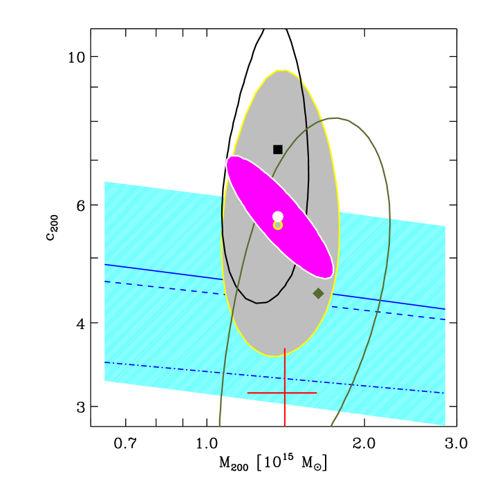
Figure 12: Best-fit solutions and 1 $\sigma$ contours in the $M_{200}$-$c_{200}$ space for the NFW $M(r)$ model (see also Table 3). Lensing analysis of U12: small magenta-filled region (with white border) and white filled dot. MAMPOSSt analysis: black vertically-elongated contour and filled square. Caustic analysis: green horizontally-elongated contour and green diamond. Joint MAMPOSSt + Caustic constraints: gray-filled region and gray dot with yellow borders. Best-fit value and 1 $\sigma$ error bars from the $\sigma_{\rm{los}}$+$r_{\nu}$ analysis: big red cross. The solid (resp. dashed) blue line and shaded cyan region represent the theoretical $cMr$ of Bhattacharya et al. (2013) for relaxed (resp. all) halos and its 1 $\sigma$ scatter. The dash-dotted blue line represents the theoretical $cMr$ of De Boni et al. (2013) for relaxed halos.

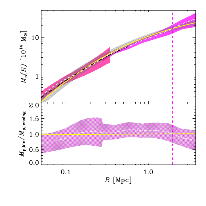
Figure 13: Top panel: The projected mass profile $M_{\rm p}(R)$ from the joint MAMPOSSt+Caustic pNFW solution (solid yellow line) within 1 $\sigma$ confidence region (hatched gray region), and from the lensing analysis of U12 (dashed white line: strong lensing analysis; dash-dotted line: weak lensing analysis, after subtraction of the contribution of the large-scale structure along the line-of-sight) within 1 $\sigma$ confidence region (hatched magenta regions). The black triple-dots-dashed line is the pNFW mass profile from U12’s analysis of Chandra data. The vertical dashed line indicates the location of $r_{\rm{200,U}}$ in both panels. Bottom panel: The ratio between the kinematic and lensing determinations of $M_{\rm p}(R)$. The white dashed and dash-dotted (resp. solid yellow) line represents the ratio obtained using the non-parametric determination (resp. the pNFW parametrization) of the lensing $M_{\rm p}(R)$. The pink hatched region represents the confidence region of this ratio for the non-parametric $M_{\rm p}(R)$ lensing solution. The horizontal black dotted line indicates the value of unity.

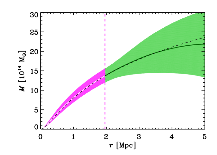
Figure 14: The solid (white and green) curve and hatched (magenta and green) region represent our fiducial $M(r)$ within 1 $\sigma$ confidence levels. This corresponds to the NFW best-fit to the lensing mass profile of U12 (white curve within magenta region) out to $r_{\rm{200,U}}$ (indicated by a vertical dashed line), and to the Caustic non-parametric mass profile (green curve within light green region) beyond that radius. The dashed black curve represents the NFW best-fit solution obtained by the combined MAMPOSSt+Caustic analysis.

In Sections 3.1 and 3.2 we have found that the NFW model is the best description of $M(r)$ among the three we have considered. This is a particularly welcome result because also U12 found that the NFW model is a good description to the cluster $M(r)$ obtained by a gravitational lensing analysis. It is therefore straightforward to compare our results with those of U12.

In Table 3 we list the values of $r_{200},r_{-2}$ and of the related parameters $M_{200},c_{200}$ of the NFW model, as obtained from the MAMPOSSt and Caustic analyses (see Sect. 3.1 and 3.2), as well as the results obtained by U12. In addition, we list the values obtained by combining the constraints from the MAMPOSSt and Caustic analyses. The combination is done by summing the $-2\ln L$ values from the MAMPOSSt analysis (where $L$ are the likelihood values) and the $\Delta\chi^{2}$ values from the NFW fit to the Caustic mass density profile, and by taking the value corresponding to the mimimum sum. To account for the fact that the two methods are largely based on the same data-set, the marginalized errors on the resulting parameters are multiplied by $\sqrt{2}$. Combining the MAMPOSSt and Caustic results allows us to reach an accuracy on the $M(r)$ parameters which is unprecedented for a kinematic analysis of an individual cluster, similar to that obtained from the combined strong and weak lensing analysis. There is a very good agreement between the $r_{200},r_{-2}$ values obtained by the combined MAMPOSSt and Caustic analyses and those obtained by the lensing analysis of U12.

Our kinematic constraints on the cluster $M(r)$ are free of the usual assumptions that light traces mass and that the DM particle and galaxy velocity distributions are identical. When dealing with poor data-sets (unlike the one presented here) one is forced to adopt simpler techniques and accept these assumptions. It is instructive to see what we would obtain in this case. We would use the sample of passive members to infer the value of $r_{200}$ from the $\sigma_{\rm{los}}$ value, as we have done in Sect. 2.1. As for the value of $r_{-2}$ we would assume it to be identical to $r_{\nu}$ (see Sect. 2.2); this is the so-called ’light traces mass’ hypothesis. There is some observational support that this assumption is verified (on average) for the passive population of cluster members (e.g. van der Marel et al. 2000; Biviano & Girardi 2003; Katgert et al. 2004). In Table 3 we list the $\sigma_{\rm{los}}$-based value of $r_{200}$, the $r_{\nu}$ value of the spatial distribution of passive cluster members, and the implied values of $M_{200},c_{200}$ (we label the method ’$\sigma_{\rm{los}}$+$r_{\nu}$’ hereafter). Formally the statistical uncertainties on these values are smaller than those of any other method. However, this comes at a price of biasing the inferred value of $c_{200}$ low, since the ’light traces mass’ hypothesis does not seem to be verified in this cluster, i.e. $r_{\rho}\neq r_{\nu}$. On the other hand, the $M_{200}$ value is in excellent agreement with those derived using more sophisticated methods.

In Fig. 12 we show the best-fit solutions and 1 $\sigma$ contours for the NFW $M(r)$ parameters $M_{200},c_{200}$, as obtained with the MAMPOSSt and Caustic analyses, as well as the results obtained by U12. Interestingly, the covariance between the errors in the $M_{200}$ and $c_{200}$ parameters is different for the different techniques (MAMPOSSt, Caustic, and lensing). We also show the results obtained from the simplified $\sigma_{\rm{los}}$+$r_{\nu}$ method and the results from the combined MAMPOSSt and Caustic solution, where we take care of drawing the contours at a level twice as high as that used for the individual MAMPOSSt and Caustic solutions.

In Fig. 12 we also show theoretical predictions for the $cMr$ of the total halo mass distribution. From the DM-only simulations of Bhattacharya et al. (2013) we show two $cMr$, one for all halos in their cosmological simulations, and another for the subset of dynamically relaxed halos. From the hydrodynamical simulations of De Boni et al. (2013) we only show the $cMr$ for relaxed halos. Our $M_{200},c_{200}$ results are in reasonable agreement with theoretical predictions. The difference between the observed and predicted $M_{200},c_{200}$ values is smaller than both the observational uncertainties and the theoretical scatter in the $cMr$. Our result is in better agreement with the theoretical prediction from the DM-only simulations of Bhattacharya et al. (2013) than with that from the hydrodynamic simulation of De Boni et al. (2013). Our result lies at the high concentration end of the allowed theoretical range, a region occupied by more dynamically relaxed halos in numerical simulations (e.g. Macciò et al. 2007; De Boni et al. 2013; Bhattacharya et al. 2013). This is consistent with the fact that this cluster was selected to be free of signs of ongoing mergers (Postman et al. 2012). Also the good agreement between the lensing, and the kinematic estimates of the cluster mass profile is an indication for dynamical relaxation. Deviation from relaxation should in fact affect the kinematic analysis but not the lensing analysis, and we should not obtain consistent results from the two analyses.

Independent constraints on the cluster $M(r)$ have also been obtained from the analysis of Chandra X-ray data by U12. The X-ray data do not allow estimating $M(r)$ beyond $r_{500}$. We can however directly compare the $M(r)$ obtained by the different methods in the radial range where they overlap. Since the lensing technique provides the projected $M(r)$, $M_{\rm p}(R)$, for the sake of comparison we also project the NFW models that provide the best-fit to the kinematic and X-ray data. In Fig. 13 we show U12’s strong and weak lensing determinations of $M_{\rm p}(R)$, within their 1 $\sigma$ confidence regions, as well as the pNFW model best-fit obtained by U12 using Chandra X-ray data, and the pNFW model best-fit we obtained by the joint MAMPOSSt+Caustic likelihood analysis. The agreement between the different mass profile determinations is very good.

Given the good consistency between the $M(r)$ parameter values obtained by the kinematic and lensing techniques, we now combine them to form a unique $M(r)$ solution. Within $r_{\rm{200,U}}$ we adopt the best-fit NFW $M(r)$ obtained by the lensing analysis of U12, since this has the smallest uncertainties, as measured by the figure of merit defined in Sect. 3.1. Beyond $r_{\rm{200,U}}$ we adopt the $M(r)$ determination obtained by the Caustic technique. In fact, the lensing analysis is limited to radii $\leq 3$ Mpc, while the Caustic $M(r)$ determination extends to $\sim$5 Mpc. Moreover, beyond $r_{\rm{200,U}}$ the lensing $M(r)$ determination is affected by the presence of a large-scale structure feature contaminating the cluster line-of-sight (U12). An additional advantage of using the Caustic $M(r)$ determination at large radii is that we do not rely on the NFW parametrization, which might not provide an adequate fit to the mass density profile of virialized halos much beyond their virial radius (Navarro et al. 1996). Since the Caustic and lensing $M_{200}$ values are consistent but not identical, we re-evaluate the Caustic $M(r)$ (and its errors) starting from $r_{\rm{200,U}}$ outwards, assuming the lensing $M_{200}$ value at $r_{\rm{200,U}}$.

The resulting mass profile is shown in Fig. 14 where we also display the joint MAMPOSSt+Caustic NFW best-fit model for comparison. It is the first time that it is possible to constrain the $M(r)$ of an individual cluster from 0 to 5 Mpc (corresponding to $2.5\,r_{200}$) with this level of accuracy. In the next Section we will use this mass profile to determine the orbits of different galaxy populations within the cluster.

4 The velocity anisotropy profile

In the previous Section we determined a fiducial mass profile (shown in Fig. 14) that we now use to determine the velocity anisotropy profiles of different cluster galaxy populations, via inversion of the Jeans equation, a problem first solved by Binney & Mamon (1982). In our analysis we solve the sets of equations of Solanes & Salvador-Solé (1990) and, as a check, also those of Dejonghe & Merritt (1992). Similarly to what was done by Biviano & Katgert (2004), our procedure is almost fully non-parametric, once the mass profile is specified. In particular, we do not fit the number density profiles (at variance with what we did in Section 2.2), but we apply the LOWESS technique (see, e.g., Gebhardt et al. 1994) to smooth the background-subtracted binned number density profiles. We then invert the smoothed profiles numerically (using Abel’s equation, see Binney & Tremaine 1987) to obtain the number density profiles in 3D. We use LOWESS also to smooth the binned $\sigma_{\rm{los}}$ profiles.

Since the equations to be solved contain integrals up to infinity, we need to extrapolate these smoothed profiles to infinite radius. In practice we approximate infinity with $R_{\infty}=30$ Mpc and we check that increasing this radius to larger values does not affect our results. We extrapolate the LOWESS smoothing of $n(R)$ beyond the last observed radius, $R_{l}$, with the following function:

$$n(R)=\eta\,(R_{\infty}-R)^{\xi}/R^{\zeta},$$ (10)

with

$$\begin{array}[]{l}\zeta=[{\rm d}\log n/{\rm d}\log R]_{R_{l}}-\xi\,R_{l}/(R_{\infty}-R_{l}),\\ \eta=n(R_{l})\,R_{l}^{\zeta}/(R_{\infty}-R_{l})^{\xi}.\end{array}$$

The only free parameter in the extrapolating function is the $\xi$ parameter. We extrapolate the LOWESS smoothing of $\sigma_{\rm{los}}$ beyond the virial radius, $r_{\rm{200,U}}$, by assuming that $\sigma_{\rm{los}}$ at $R_{l}$ is a fixed fraction of the peak $\sigma_{\rm{los}}$ value, and by making a log-linear interpolation between $\log r_{200}$ and $\log R_{l}$. The $\beta(r)$ solutions are rather insensitive to different choices of the extrapolation parameters (any change is well within the error bars – see below).

The dominant source of error on $\beta(r)$ arises from the uncertainties in $\sigma_{\rm{los}}$. It is however virtually impossible to propagate the errors on $\sigma_{\rm{los}}$ through the Jeans inversion equations to infer the uncertainties on the $\beta(r)$. We then estimate these uncertainties the other way round. We modify the $\beta$ profile in a generic way as follows, $\beta(r)\rightarrow\beta(r)+\varepsilon_{1}+\delta_{1}\,r$, and $\beta(r)\rightarrow\varepsilon_{2}\,\beta(r)+\delta_{2}$. We then compute the predicted $\sigma_{\rm{los}}$ profiles for all values of $\{\varepsilon_{1},\delta_{1}\}$ and $\{\varepsilon_{2},\delta_{2}\}$ in a wide grid, using the equations of van der Marel (1994). The range of acceptable $\beta(r)$ profiles is determined by a $\chi^{2}$ comparison of the resulting $\sigma_{\rm{los}}$ profiles with the observed one.

Figure 15: The velocity-anisotropy profile, $\beta(r)$, of different cluster galaxy populations. Top panel: all cluster members. The solid (white) curve is the solution of the inversion of the Jeans equation adopting the reference mass profile defined in Section 3.3. The hatched (gray) region indicates the 1 $\sigma$ confidence region around this solution. For comparison, three $\beta(r)$ models are shown (black curves). They correspond to the best-fit $\beta(r)$ models of the MAMPOSSt analysis for a NFW $M(r)$ model (see Sect. 3.1), namely (from top to bottom at small radii) the C, T, and O model. In both panels, the vertical dashed and dash-dotted (magenta) lines indicate the location of $r_{-2}$ and $r_{200}$, respectively, and the horizontal dotted line indicates $\beta=0$. Bottom panel: passive and SF cluster members, separately. The red solid (resp. blue dash-dotted) curve and orange (resp. cyan) hatched region represent the solution of the inversion of the Jeans equation within the 1 $\sigma$ confidence region for passive (resp. SF) cluster members.

The $\beta(r)$ we obtain by this procedure using all cluster members is shown in Fig. 15 (top panel). This is the highest-$z$ determination of an individual cluster $\beta(r)$ so far, and one of the few available in the literature in a non-parametric form (Biviano & Katgert 2004; Benatov et al. 2006; Natarajan & Kneib 1996; Hwang & Lee 2008; Lemze et al. 2011). It is isotropic near the center, then it gently increases with radius, reaching a mild radial anisotropy, $\beta\simeq 0.5$ at $\simeq r_{200}$. Constant, isotropic velocity anisotropy is ruled out.

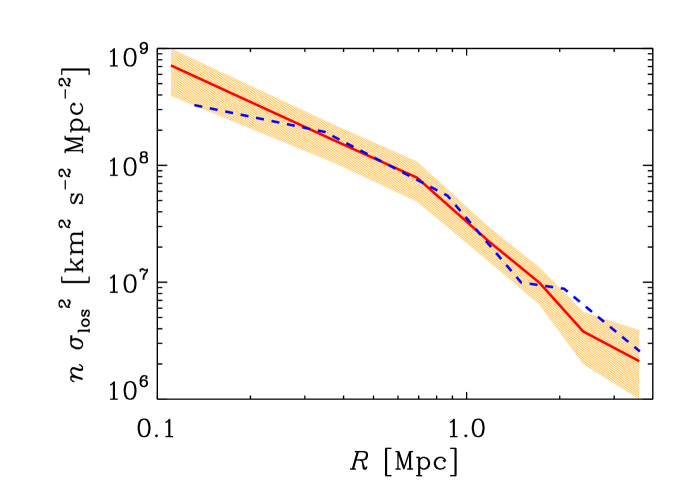
Figure 16: Consistency of the shapes of the $n(R)\,\sigma_{\rm{los}}^{2}(R)$ profiles of the passive (solid red line) and SF (dashed blue line) cluster galaxy populations. The profile for the SF galaxy population has been multiplied by 3.7 to allow for a direct comparison with the profile of the passive galaxy population. The hatched (orange) region indicates the 1 $\sigma$ confidence level of the profile of the passive population (that for the SF population is not shown, but it is much larger).

In Fig. 15 we also display the best-fit $\beta(r)$ model obtained by running the MAMPOSSt method with a NFW mass profile model (see Sect. 3.1). All MAMPOSSt parametrized solutions are consistent with this non-parametric determination over most of the covered radial range. Note that the MAMPOSSt best-fit T $\beta(r)$ model is identical to the model that has been shown (Mamon & Łokas 2005; Mamon et al. 2010, 2013) to adequately describe the $\beta(r)$ of cluster-mass halos extracted from cosmological simulations.

In the bottom panel of Fig. 15 we show the $\beta$ profiles of the passive and, separately, SF subsamples (defined in Section 2.1). It is the first time that $\beta(r)$ is determined separately for these two populations in an individual cluster. The two profiles appear very similar, and therefore also very close to the $\beta(r)$ of all galaxies. Splitting the sample in two clearly increases the error bars, so the passive and SF $\beta(r)$ are formally consistent with isotropic orbits at all radii.

The remarkable similarity of the $\beta(r)$ of passive and SF galaxies may seem unexpected given that their $n(R)$ are quite different (see Fig. 7). However, the normalization of $n(R)$ is irrelevant in the Jeans inversion equation and what matters is the combination $n(R)\,\sigma_{\rm{los}}^{2}(R)$ (sometimes called ’projected pressure’), and the normalization of $\sigma_{\rm{los}}(R)$. We have already seen that the values of $\sigma_{\rm{los}}$ for the passive and SF cluster galaxy populations are quite similar (see Table 1). In Fig. 16 we show that also the shape of the $n(R)\,\sigma_{\rm{los}}^{2}(R)$ is rather similar for the two populations, so the similarity of the passive and SF $\beta(r)$ is not unexpected.

5 $Q(r)$ and the $\gamma$-$\beta$ relation

With $M(r)$ and $\beta(r)$ we are now in the position to investigate the $Q(r)$ behavior and the existence of the $\gamma$-$\beta$ relation (see Section 1). It is the first time that these relations are tested observationally in a galaxy cluster. Both relations depend on the mass density profile, $\rho(r)$, which is the same for all tracers of the gravitational potential, but they also depend on other quantities, the velocity dispersion and velocity anisotropy profiles, which might in principle be different for different tracers. Clearly we do not have access to these profiles for the DM particles, since they are not observables, so we determine $Q(r)$ and the $\gamma$-$\beta$ relation separately for different classes of tracers, namely all, passive, and SF cluster members.

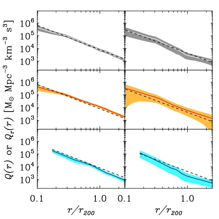
Figure 17: The pseudo phase-space density profiles $Q(r)\equiv\rho/\sigma^{3}$ (left panels) and $Q_{\rm r}(r)\equiv\rho/\sigma_{\rm{r}}^{3}$ (right panels), as a function of clustercentric radius $r$, within 1 $\sigma$ confidence regions (shaded area) for all (top panels), passive (middle panels), and SF (bottom panels) cluster members. The dashed lines are fixed-slope best-fit relations $Q(r)\propto r^{-1.84}$ and $Q_{\rm r}(r)\propto r^{-1.92}$ to the sample of all galaxies, where the slopes are those found by Dehnen & McLaughlin (2005) using numerically simulated halos.

In Fig. 17 we display $Q(r)\equiv\rho/\sigma^{3}$ (left panels), and $Q_{\rm r}(r)\equiv\rho/\sigma_{\rm{r}}^{3}$ (right panels), for all, passive, and SF cluster members separately. The mass density profile $\rho(r)$ is obtained from our fiducial mass profile (see Sect. 3) and $\sigma(r)$ and $\sigma_{\rm{r}}(r)$ are obtained from the inversion of the Jeans equation (see Sect. 4). The error bars are derived from the uncertainties on $\rho(r)$ and $\beta(r)$, through a propagation of error analysis; $\sigma_{\rm{r}}(r)$ is affected by much larger uncertainties than $\sigma(r)$ because of the large uncertainties on $\beta(r)$, i.e. we know the total velocity dispersion better than we know its separate components.

In Figure  17 we also show the fixed-slope best-fit relations $Q(r)\propto r^{-1.84}$ and $Q_{\rm r}(r)\propto r^{-1.92}$ using the sample of all galaxies, where the slopes are those found by Dehnen & McLaughlin (2005) for DM particles in numerically simulated halos. The sample of all members obey both theoretical relations for $Q(r)$ and $Q_{\rm r}(r)$ within the error bars. Also the subsample of passive members follows the theoretical relations, while the subsample of SF galaxies follows the theoretical relations only at $r/r_{200}\la 0.7$.

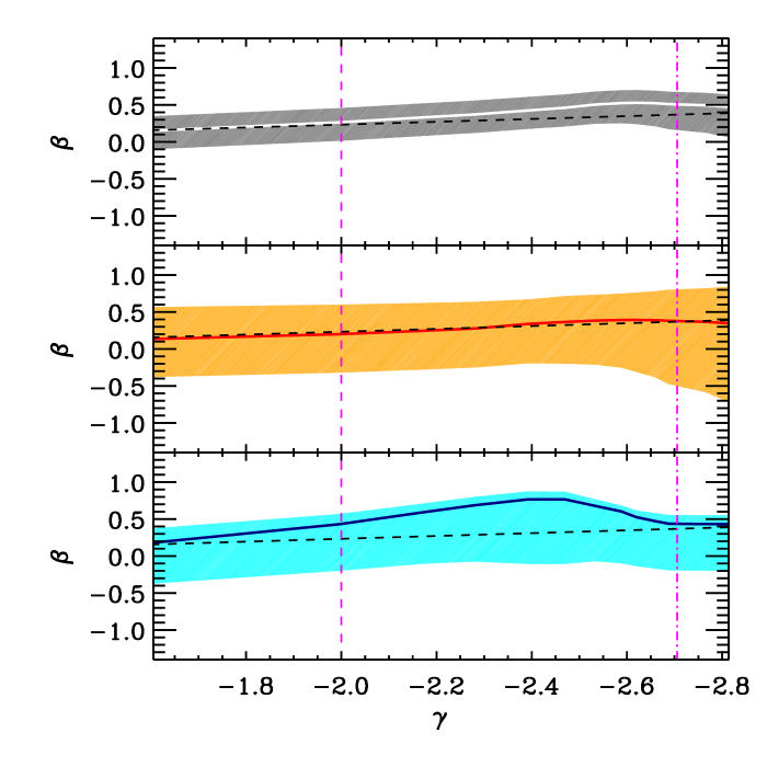
Figure 18: The relations between $\beta(r)$ and the logarithmic derivative of the total mass density profile, $\gamma(r)$, for all, passive, and SF member galaxies (top, middle, and bottom panel, respectively), within 1 $\sigma$ confidence regions (shaded regions), and the theoretical $\gamma$-$\beta$ relation of Hansen & Moore (2006) (dashed line). The vertical lines indicate the location of $r_{-2}$ (dashed) and $r_{200}$ (dash-dotted).

In Fig. 18 we show $\beta(r)$ vs. the logarithmic derivative of the mass density profile, $\gamma(r)$, for all, passive, and SF members, separately, and the theoretical $\gamma$-$\beta$ relation of Hansen & Moore (2006, see eq. 2). The theoretical relation is consistent with the data within the observational error bars for the full sample of members. Passive galaxies obey the theoretical $\gamma$-$\beta$ relation very well at all radii. On the other hand, the observed relation for SF galaxies deviates from the theoretical one, especially at large radii, but this deviation is not statistically significant, given the rather large observational uncertainties.

6 Discussion

6.1 The mass profile

Using a large spectroscopic sample of $\sim 600$ cluster members as tracers of the gravitational potential we have determined the $M(r)$ of the $z=0.44$ MACS J1206.2-0847 cluster to an accuracy close to that reached by the combined strong+weak lensing analysis of U12, and over a wider radial range, reaching out to 5 Mpc (corresponding to $2.5\,r_{200}$). The determination of a cluster $M(r)$ to such a high level of accuracy and over such a wide radial range is unprecedented for this redshift.

For the $M(r)$ determination we have used two kinematics-based methods, MAMPOSSt and Caustic. This is the first application of the new MAMPOSSt method to an observed cluster. MAMPOSSt allows to determine $M(r)$ in the cluster virial region, where the Caustic method suffers from systematics, and Caustic allows to determine $M(r)$ beyond the virial region, where MAMPOSSt is not fully applicable because of possible deviations from dynamical equilibrium. The two methods are therefore complementary.

The MAMPOSSt analysis indicates that the cluster $M(r)$ is best fitted by the NFW or by the Einasto model, although we cannot reject any of the other mass models we have considered, Hernquist, Burkert, and SIS. The SIS model best-fit requires however a very small value of the core radius (see Table 2). The Caustic analysis shows that the NFW model provides a reasonable fit at least out to $\sim 2\,r_{200}$. Beyond that radius the uncertainties in the Caustic $M(r)$ determination become very large and constraints on the shape of the mass profile are too loose (see Fig. 14).

Previous analyses of cluster mass profiles traced by galaxy kinematics have generally found good agreement with the NFW model (see the review of Biviano 2008, and references therein) as we find for MACS J1206.2-0847. The Burkert model was however found to provide a somewhat better fit to the stacked $M(r)$ of the ENACS data-set (Katgert et al. 1998) by Biviano & Salucci (2004) and cored models were not excluded by the analysis of a cluster sample extracted from the 2dFGRS (Colless et al. 2001) by Biviano & Girardi (2003). Biviano & Girardi (2003) have also found the $M(r)$ slope to be consistent with that of NFW up to $\sim 2r_{200}$; beyond that radius, the slope may become intermediate between those of the NFW and Hernquist models, according to the analysis of the CAIRNS cluster sample (Rines et al. 2003b). These previous results were based on the combination or averaging of several cluster data-sets, since the individual cluster statistics was insufficient to constrain $M(r)$, unlike in our case.

The best-fit NFW model obtained by combining the results of the two kinematic methods (via a weighted average) is very close to the best-fit NFW model obtained by the combined strong and weak lensing analysis of U12 (see Fig. 13). The accuracy level we reach on the $M(r)$ parameters is close to that reached by the combined strong and weak lensing analysis. There is also a very good agreement with the $M(r)$ estimate within $\sim r_{500}$ obtained by U12 using Chandra X-ray data.

The excellent agreement we have found between the kinematically-derived $M(r)$, the $M(r)$ from lensing, and the $M(r)$ from X-ray indicates that our and U12’s results are free from possible systematics. It also indicates that MACS J1206.2-0847 is dynamically relaxed.

The $\sigma_{\rm{los}}$-based $r_{200}$ estimate is also in agreement with our other estimates (Table 3 and Fig. 12). This constrains the velocity dispersion of passive cluster members to be within $\pm 10$% of that of DM particles, in agreement with the results of numerical simulations (see, e.g., Fig. 8 in Munari et al. 2013).

Cluster concentrations may be affected by major mergers (Hoffman et al. 2007) and/or baryon cooling (Gnedin et al. 2004; Duffy et al. 2010; Rasia et al. 2013) which tends to steepen the $cMr$ (Fedeli 2012). Early adiabatic compression of galactic DM (Barkana & Loeb 2010) can increase the concentration. Dynamical friction acting on orbiting galaxies can pump energy into the diffuse DM component and flatten the inner density slope (El-Zant et al. 2004), and this flattening can be interpreted as a decrease in concentration (Ricotti et al. 2007). The difference in the $cMr$ of relaxed and unrelaxed halos in simulations suggests that the average effect of mergers on concentrations is not very strong (see, e.g., De Boni et al. 2013; Bhattacharya et al. 2013, see also Fig. 12). Baryonic processes appear to have a stronger effect, as can be seen by comparing the $cMr$ of De Boni et al. (2013), obtained on hydrodynamical simulations, and that of Bhattacharya et al. (2013), obtained on DM-only simulations (see Fig. 12).

The $M(r)$ of MACS J1206.2-0847 has a concentration $c_{200}=6\pm 1$, slightly higher than the average for halos at the same $z$ and of the same mass ($M_{200}=(1.4\pm 0.2)\times 10^{15}\,M_{\odot}$) extracted from cosmological numerical simulations (De Boni et al. 2013; Bhattacharya et al. 2013), but well within the scatter of the theoretical $cMr$ (see Fig. 12). The substantial agreement between the observed and theoretically predicted concentrations argues against an alignment of the cluster line-of-sight and major axis. This is also suggested by the fact that the cluster appears somewhat elongated in projection (U12).

Our result for $c_{200}$ is consistent with others obtained from analyses of the kinematics of stacked cluster samples, both at low- (Katgert et al. 2004; Biviano & Salucci 2006; Łokas et al. 2006b) and high-redshift (Biviano & Poggianti 2009). The analyses of the kinematics of individual clusters have found concentrations both in line (Łokas et al. 2006b; Rines & Diaferio 2006) and above the theoretical expectations (Łokas & Mamon 2003; Łokas et al. 2006a; Wojtak & Łokas 2007; Lemze et al. 2009; Wojtak & Łokas 2010; Abdullah et al. 2011).

The concentration of cluster galaxies (both all and only the passive ones) in MACS J1206.2-0847 is smaller than that of the total mass. Assuming that light traces mass would then lead to an erroneous mass profile determination. The concentration we find for the passive galaxies, $r_{200}/r_{\nu}=3.1\pm 0.7$, is close to the average found by Lin et al. (2004) for K-band-selected galaxies in nearby clusters, $c_{200}=2.9$. The concentration of the luminosity density profile of cluster galaxies is only $\sim 10$% higher than the concentration of their number density profile, indicating little evidence for mass segregation. The ratio of the concentrations of the total mass and the passive galaxies is $1.8\pm 0.4$, close to that found by Biviano & Poggianti (2009) for a stack of nearby clusters (1.7), but much higher than that found by the same authors for a stack of $z\sim 0.55$ clusters (0.4). Other studies have found this ratio to be closer to unity (Carlberg et al. 1997a; van der Marel et al. 2000; Biviano & Girardi 2003; Katgert et al. 2004; Rines et al. 2004). Possibly the relative concentration of total mass and cluster galaxy distribution is related to the assembly history of a cluster or to dynamical processes affecting the survival of galaxies near the center, such as merging with the central BCG or tidal stripping. Extending the analysis presented in this paper to other clusters may help understand the physical origin of the relative concentrations of mass and galaxy distribution in clusters.

6.2 The velocity anisotropy profiles

We have determined the velocity anisotropy profiles, $\beta(r)$, of passive and SF members, separately, for the first time for an individual cluster. This was done from the inversion of the Jeans equation, using our best guess for $M(r)$, derived from the combination of the best-fit NFW $M(r)$ from the lensing analysis of U12 within $r_{\rm{200,U}}$ and the Caustic $M(r)$ outside. MACS J1206.2-0847 is the highest-$z$ cluster for which $\beta(r)$ has been determined, and one of the few at all redshifts.

In our analysis we have assumed spherical symmetry. The analysis of numerically simulated halos by Lemze et al. (2012) has shown that this assumption has almost no effect on the determination of $\beta(r)$ within the virial radius.

We have found that the $\beta(r)$ of all cluster members is consistent with that of cosmological halos in numerical simulations (Mamon & Łokas 2005; Mamon et al. 2010, 2013, see Fig. 15, top panel). It is not consistent with isotropy at all radii, but only up to $\sim r_{-2}$, then it increases to more radial anisotropy.

The $\beta(r)$ for passive and SF cluster members are almost identical (and therefore also almost identical to the $\beta(r)$ of all cluster members). This is quite remarkable given that the two cluster populations have different $n(R)$, i.e. they occupy different regions in the cluster. However, the $\sigma_{\rm{los}}$ of the two populations are not significantly different (see Table 1), and the $n(R)$ and $\sigma_{\rm{los}}(R)$ of the two populations combine to produce $n(R)\,\sigma_{\rm{los}}^{2}(R)$ profiles of similar shapes (see Fig. 16). Hence the observable that enters the Jeans equation inversion (by which we estimate $\beta(r)$) is very similar for the two populations.

This common shape of the orbital distribution of cluster galaxies could be the result of violent relaxation followed by smooth accretion (Lapi & Cavaliere 2009). Violent relaxation is expected to occur at higher redshifts, and isotropize orbits, and therefore should concern the more central cluster regions. Galaxies that were accreted by the cluster after the end of violent relaxation, would retain their slightly radial orbital distribution, producing the external $\beta(r)$. Yet another process capable of isotropizing the initial radial orbits of infalling galaxies is radial orbit instability (ROI, see, e.g., Bellovary et al. 2008).

To understand which is the physical process that shapes the orbits of galaxies in clusters we must study the evolution of $\beta(r)$. Most previous observational determinations of $\beta(r)$ have been based on stacked clusters or have been obtained by assuming a fixed model shape of $\beta(r)$. The whole cluster population has been found to move on either isotropic (van der Marel et al. 2000; Rines et al. 2003b; Hwang & Lee 2008), or mildly radial orbits (Łokas et al. 2006b) with a general increase of $\beta(r)$ from nearly isotropic orbits near the center to moderate radial anisotropy outside (Benatov et al. 2006; Lemze et al. 2009; Wojtak & Łokas 2010), similar to the profile we find for MACS J1206.2-0847. The early-type, red, passive cluster population has generally been found to move on isotropic orbits (Carlberg et al. 1997b; Biviano 2002; Łokas & Mamon 2003; Katgert et al. 2004; Hwang & Lee 2008), while the late-type, blue, SF cluster population has been found to move on slightly radial orbits (Biviano & Katgert 2004; Hwang & Lee 2008). The $\beta(r)$ of SF galaxies in the nearby clusters analyzed by Biviano & Katgert (2004) is isotropic at radii $r<r_{200}/2$, then it becomes more radial.

Comparison with the $\beta(r)$ of lower-$z$ clusters suggests that passive galaxies undergo evolution of their orbits, more than SF galaxies, and the orbits tend to become more isotropic with time. Our result thus confirms the suggestion of Biviano & Poggianti (2009), which was based on a stacked sample of clusters at $z\sim 0.5$ (see also Benatov et al. 2006). Since violent relaxation is a process that occurs on relatively short, dynamical timescales, and at high $z$, one could argue that the secular evolution of galaxy orbits toward isotropy is related instead to a different process, possibly ROI. At variance with violent relaxation, ROI continues even after the cluster has virialized (Barnes et al. 2007). If the ROI timescale is long, this could explain why we see orbital evolution for the passive cluster members, and not for the SF ones, since SF galaxies would have the time to transform into passive before ROI modifies their orbits.

Another process by which cluster galaxies could undergo orbital evolution is via interaction with the ICM (Dolag et al. 2009). Since this process also quenches star-formation, it could naturally explain why we observe $\beta(r)$ evolution for the quenched (passive) cluster galaxies, and not for the SF ones. The timescale and importance of this process needs however to be quantified to allow a more relevant comparison with observational results.

Other results from numerical simulations are contradictory on the topic of $\beta(r)$ evolution. Lemze et al. (2012) do not find significant evolution of $\beta(r)$ with redshift. Munari et al. (2013) finds that $\beta(r)$ for massive clusters becomes mildly more radial at higher redshift. Their result is consistent with that of Wetzel (2011) who finds that the orbits of satellites at the moment of their infall within larger host halos are more radial at higher $z$. On the other hand, Iannuzzi & Dolag (2012) find the opposite redshift trend.

To better understand the issue of $\beta(r)$ evolution, one needs a much larger sample of clusters at different redshifts. There is considerable variance in the shapes of the $\beta(r)$ of cluster-size halos extracted from numerical simulations, even if located at the same $z$ (see, e.g., Fig.1 in Mamon et al. 2013). Possibly, the $\beta(r)$ shape is related to the shape of $M(r)$, and one cannot treat them separately. Below, we discuss this point in detail.

6.3 The pseudo-phase-space density profiles

In Section 6.2 we have argued for possible mechanisms capable of explaining the $\beta(r)$ of different cluster populations. Combining our knowledge of $M(r)$ and $\beta(r)$ can shed more light on this topic. For the first time ever, we have determined $Q(r)$, $Q_{\rm r}(r)$, and the $\gamma$-$\beta$ relation observationally, separately for all, passive, and SF cluster members. All cluster members, and also, separately, the subsamples of passive members, obey the theoretical relations within the observational error bars (see Fig. 17 and Fig. 18). Only for SF members there is some tension between the observed and theoretical relations, even if only at large radii, $\ga 0.7\,r_{200}$.

Dehnen & McLaughlin (2005) have shown that, given the $\gamma$-$\beta$ relation and the Jeans equation for dynamical equilibrium, $Q_{\rm r}(r)$ is a power-law in $r$, with an exponent related to $\beta(0)$. Based on their finding Dehnen & McLaughlin (2005) argue as follows. Violent relaxation would tend to create a scale-invariant phase-space density (since the process is driven by gravity alone), hence $Q_{\rm r}(r)\propto r^{\alpha}$. Dynamical equilibrium would then force $\alpha$ to approach a critical value, from which results the particular form of the $\rho(r)$ of cosmological halos. A value $\beta(0)\simeq 0$ with radially increasing $\beta(r)$ gives the $\alpha$ observed in numerical simulations. The form of $\beta(r)$ could therefore result from the halo violent relaxation followed by its dynamical equilibrium (Hansen 2009).

If this argumentation is correct, passive members of MACS J1206.2-0847 have undergone violent relaxation and have reached dynamical equilibrium, while SF members seem to have not, although the current uncertainties are still rather large. Moreover, one would be tempted to conclude that baryonic processes are not particularly important in shaping the dynamical structure of galaxy clusters, since they are unable to change the $Q(r)$ of galaxies that have undergone violent relaxation.

Comparison of the $Q(r)$ and $Q_{\rm r}(r)$ for a sample of clusters at different redshifts is needed for further insight. To our knowledge, there is only another cluster for which a similar analysis is being done (Munari, Biviano & Mamon, in prep.). Also in this nearby ($z=0.09$) cluster, the $Q(r)$ of red galaxies is in agreement with the theoretical prediction, and that of blue galaxies is not. The lack of evolution in the $Q(r)$ of passive galaxies is perhaps surprising, since SF galaxies become passive with time, and their $Q(r)$ is different from that of passive galaxies. Perhaps as SF galaxies get quenched, their $Q(r)$ evolves and approaches the theoretical prediction, but this would contradict the idea that $Q(r)$ is shaped by the process of violent relaxation alone. Another possibility is that the fraction of late-quenched galaxies in the spectroscopic data-sets of passive cluster members is small because late-quenched galaxies are fainter than the more pristine cluster passive members. This can happen because of downsizing (e.g. Neistein et al. 2006), or because of the effects of tidal stripping (e.g. Balogh et al. 2002). Drawing conclusions on the basis of only two clusters is however premature. To shed more light on this topic $Q(r)$ must be determined for more clusters, over a range of redshifts, and for galaxies of different luminosities.

7 Conclusions

We have analyzed the internal dynamics of the MACS J1206.2-0847 cluster at $z=0.44$, based on a large spectroscopic sample of more than 2500 galaxies in its field, mostly from VLT/VIMOS data obtained in the context of the ESO large programme 186.A-0798. From this sample we have identified $\sim$600 cluster members. This is the largest spectroscopic sample for cluster member galaxies at $z>0.4$, and one of the largest available at any $z$. Using this sample, we have applied the Caustic and, for the first time on an observed cluster, the MAMPOSSt method, to determine the cluster mass profile, $M(r)$. These two methods do not rely on the assumption that the spatial and/or velocity distributions of cluster galaxies are identical to those of the DM particles.

We have found an excellent agreement between the $M(r)$ determined using the projected phase-space distribution of cluster galaxies and those determined by U12, who used a combined strong and weak gravitational lensing analysis and Chandra X-ray data. This agreement indicates that possible systematic biases in our dynamical analyses have been properly accounted for, and that the cluster is in a relaxed dynamical state. The cluster $M(r)$ is best described by a NFW model, but other mass profile models provide acceptable fits to our data. The observed concentration of the best-fit NFW model is slightly above current theoretical predictions, but not significantly so. The spatial distribution of all and passive cluster members is less centrally concentrated than the total mass. Using the velocity dispersion of passive cluster members to estimate the cluster mass gives a value in agreement with those obtained by the other, more sophisticated, analyses. This suggests that the bias between the velocity dispersion of passive cluster members and DM particles is small, $\la 10$%.

We have defined a fiducial $M(r)$ from the combination of those obtained with the lensing and kinematic analyses, spanning a radial range from the center to $\sim$5 Mpc (corresponding to $2.5\,r_{200}$). To our knowledge, this is currently the most accurate determination of a cluster $M(r)$ over this radial range. We have used it to invert the Jeans equation and determine the velocity anisotropy profiles, $\beta(r)$, for all cluster members, and, separately, for passive and SF cluster members. This is the highest-$z$ individual cluster for which $\beta(r)$ has been determined so far, and the only one for which $\beta(r)$ has been determined separately for both passive and SF galaxies. We have found almost identical velocity anisotropy profiles for the different cluster galaxy populations, isotropic near the center (within $\sim r_{-2}$) and increasingly radially anisotropic outside. This profile resembles that of DM particles in halos extracted from cosmological numerical simulations. Comparison with nearby clusters suggests evolution of the orbital profile of passive cluster members, but the physical mechanism driving this evolution remains to be identified.

From the mass density profile and $\beta(r)$, thanks to the quality of our $M(r)$ and the size of our spectroscopic data-set, we have been able to determine the pseudo phase-space density profiles $Q(r)$ and $Q_{\rm r}(r)$ and the $\gamma$-$\beta$ relation. These are the first observational determinations of these profiles and relation for a galaxy cluster. They are consistent with the theoretical expectations in particular for the passive cluster members. This is probably an indication that these galaxies were in the cluster at the time of violent relaxation. Marginal deviation from the theoretical relations is observed instead for the SF cluster members, suggesting that they are a more recently accreted population.

The cluster studied in this paper is part of a sample of 14 clusters from the CLASH-VLT Large Programme with the VIMOS spectrograph, which we expect to be completed in 2014. In this paper we have shown that with a spectroscopic sample of this size it is possible to constrain a cluster $M(r)$ to an accuracy similar to that achievable by a detailed, combined strong + weak lensing analysis. It is also possible to constrain the orbits of different cluster galaxy populations in a non-parametric way by direct inversion of the Jeans equation. Combining results from $M(r)$ and $\beta(r)$ it is possible to test dynamical relations that inform us on the way cosmological halos evolve and organize internally. We will extend this analysis to all the CLASH clusters with sufficient spectroscopic coverage in the near future, and this will allow us to explore the variance in the cluster dynamical states, the $cMr$ for the total mass and the different galaxy populations, and the universality of the $Q(r)$ and $\beta$-$\gamma$ dynamical relations. Stacking dynamically-relaxed clusters together could in the end even allow us to constrain the equation of state of DM by comparison of the kinematically-derived and lensing-derived mass profiles (Faber & Visser 2006; Serra & Domínguez Romero 2011).

Appendix A The effects of different cluster membership definitions

The determinations of $M(r)$ and $\beta(r)$ described in Sect. 3 and 4 are based, at least in part, on the sample of cluster members defined by the P+G procedure (see Sect. 2.1). Here we examine how a different cluster membership definition affects our results. For this, we here consider the membership definition obtained with the Clean method instead of the P+G method. The two methods use very different approaches for the identification of cluster members, as described in Sect. 2.1.

In Table 4 we list the fractional differences and associated 1 $\sigma$ uncertainties of the $r_{200},r_{-2}$ and $r_{\nu}$ determinations obtained by using the two samples of cluster members identified with the P+G and the Clean methods. The effects of changing the method of membership selection are marginal, as all changes are within 1 $\sigma$.

Table 4: The effects of changing the member selection method (Clean vs. P+G).

Method	Sample	Clean/P+G
Quantity: $r_{200}$
From $\sigma_{\rm{los}}$	$R\leq 1.98$ Mpc (passive only)	$1.07\pm 0.07$
MAMPOSSt	$0.05\leq R\leq 1.96$ Mpc	$1.04\pm 0.12$
Caustic	$R\leq 2\times 1.96$ Mpc	$1.03\pm 0.22$
Quantity: $r_{-2}$
MAMPOSSt	$0.05\leq R\leq 1.96$ Mpc	$0.80\pm 1.14$
Caustic	$R\leq 2\times 1.96$ Mpc	$1.00\pm 0.53$
Quantity: $r_{\nu}$
–	$R\leq 1.96$ Mpc	$0.96\pm 0.20$
–	$R\leq 1.96$ Mpc (passive only)	$0.91\pm 0.19$
–	$R\leq 1.96$ Mpc (SF only)	$1.10\pm 0.37$

The $r_{200}$ estimates are all slightly increased when adopting the Clean method instead of the P+G method, and this happens because of the 8 galaxies with high absolute values of ${\rm v}_{{\rm rf}}$ near the cluster center selected as members by the Clean method but not by the P+G method (see Fig. 2). Since 7 of these 8 galaxies are passive, the effects of the different membership selection are stronger on the quantities derived using only passive galaxies.

The inclusion of these 8 galaxies in the sample of cluster members causes a higher velocity dispersion estimate near the center, and therefore a steeper $\sigma_{\rm{los}}$ profile. To accommodate for the steeper $\sigma_{\rm{los}}$ profile near the center, the MAMPOSSt analysis forces more concentrated mass profiles, with 20–25% smaller $r_{-2}$ estimates. However, given the large uncertainties on the $r_{-2}$ estimates these changes are far from being significant. The Caustic $M(r)$ estimate is less affected, because i) it is only partially based on the membership selection within the virial radius, and ii) it uses all galaxies (and not only members) also beyond the virial radius.

The $r_{\nu}$ estimates depend very little on which membership selection is chosen, because i) they are based not only on the sample of spectroscopic members but also on the sample of $z_{\rm{p}}$-selected members, and ii) the inclusion of the 8 additional members near the center has a smaller impact on $n(R)$ than it has on $\sigma_{\rm{los}}(R)$.

Given the marginal changes in the MAMPOSSt and Caustic estimates of $r_{200}$ and $r_{-2}$, using the Clean-based membership determination instead of the P+G-based one, we still find consistency between the $M(r)$ obtained via the MAMPOSSt and Caustic method and that of U12. As a consequence, we would still adopt the $M(r)$ of U12 within $r_{\rm{200,U}}$ and the Caustic $M(r)$ at larger radii, and the resulting $M(r)$ would be almost identical to the one we adopted using the P+G membership determination (Sect. 3.3).

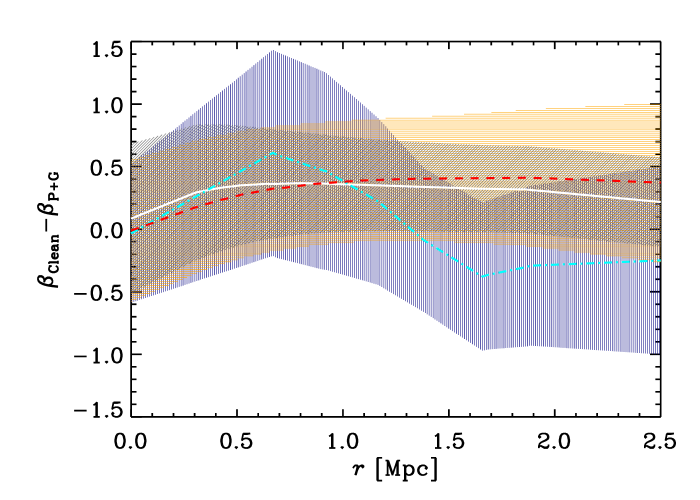
Figure 19: The difference of the $\beta(r)$ determined using the Clean and P+G samples of members. The solid (white), dashed (red), and dash-dotted (cyan) curves are for all, passive, and SF galaxies, respectively. 1 $\sigma$ intervals on the differences are shown as shaded regions, with 45, 0, and 90 degrees orientation of the (gray, orange, blue) shading for all, passive, and SF galaxies, respectively.

The $\beta(r)$ profiles resulting from the inversion of the Jeans equation are marginally affected mostly because of the steepening of the $\sigma_{\rm{los}}$ profile. Given that the adopted $M(r)$ is almost unchanged with respect to the case of P+G membership selection, the steepening of $\sigma_{\rm{los}}(R)$ near the center must be compensated by an increased radial anisotropy. This concerns mostly the passive galaxies. The differences between the $\beta(r)$ obtained using the Clean-based sample of members and those obtained using the P+G-based sample of members are consistent with zero within 1 $\sigma$ for all cluster populations and at all radii (see Fig. 19).

We conclude that our results do not change significantly if we use the Clean instead of the P+G method for membership selection.

Appendix B Comparison with other cluster mass estimates from the literature

We here compare our results to those obtained by Foëx et al. (2012) and Ebeling et al. (2009). In both cases their data were of insufficiently quality to constrain both $r_{200}$ and $r_{-2}$, so we only compare the $r_{200}$ values.

The weak lensing $r_{200}$ estimate of Foëx et al. (2012), $2.03_{-0.09}^{+0.11}$ Mpc, is in good agreement with our estimate.

Ebeling et al. (2009) have estimated the cluster mass in three ways; i) by strong lensing, ii) by an hydrostatic equilibrium analysis of the X-ray emitting intra-cluster medium, and iii) by the virial theorem. Their strong lensing mass estimate, $1.12\times 10^{14}M_{\odot}$ within 0.12 Mpc from the cluster center, is in agreement with our determinations. By applying a scaling relation to the cluster X-ray temperature Ebeling et al. (2009) obtain an approximate value of $r_{200}$, $2.3\pm 0.1$ Mpc, in disagreement with our estimate. They then estimate the cluster mass within this radius using an isothermal $\beta$ model profile, $1.7\pm 1\times 10^{15}M_{\odot}$. This $M_{200}$ estimate corresponds to a $r_{200}$ estimate of 2.1 Mpc, different from their initial estimate, but still above our best estimate. Had they iterated their eq.(5) they would have obtained a concordant pair of $r_{200},M_{200}$ estimates with a final value of $r_{200}$ of 2.03 Mpc, closer to our best estimate.

The virial theorem mass estimate of Ebeling et al. (2009) is instead grossly discrepant with any other estimate discussed so far. This appears to be due to a combination of causes. First, their membership selection is too simplistic since it does not take into account the radial position of galaxies. As a consequence, they obtain a much larger velocity dispersion estimate than we do, 1581 km s^-1(compare to the values in Table 1). Their large estimate is also due to the fact that $\sigma_{\rm{los}}$ is decreasing with $R$ (see Fig. 3) and their spectroscopic sample does not reach $r_{\rm{200,U}}$. Other causes that lead Ebeling et al. (2009) to overestimate the cluster mass using the virial theorem are the neglect of the surface-pressure term (The & White 1986), and the use of a spatially incomplete sample in the estimate of the projected harmonic mean radius (see Biviano et al. 2006).