The UVES Large Program for Testing Fundamental Physics II:
Constraints on a Change in Towards Quasar HE 00271836††thanks: Based on data obtained with
UVES at the Very Large Telescope of the European Southern Observatory
(Prgm. ID 185.A-0745)
Abstract
We present an accurate analysis of the absorption lines from the 2.4018 damped system towards HE 00271836 observed with the Very Large Telescope Ultraviolet and Visual Echelle Spectrograph (VLT/UVES) as a part of the European Southern Observatory Large Programme ”The UVES large programme for testing fundamental physics” to constrain the variation of proton-to-electron mass ratio, . We perform cross-correlation analysis between 19 individual exposures taken over three years and the combined spectrum to check the wavelength calibration stability. We notice the presence of a possible wavelength dependent velocity drift especially in the data taken in 2012. We use available asteroids spectra taken with UVES close to our observations to confirm and quantify this effect. We consider single and two component Voigt profiles to model the observed absorption profiles. We use both linear regression analysis and Voigt profile fitting where is explicitly considered as an additional fitting parameter. The two component model is marginally favored by the statistical indicators and we get = ppm. When we apply the correction to the wavelength dependent velocity drift we find = ppm. It will be important to check the extent to which the velocity drift we notice in this study is present in UVES data used for previous measurements.
keywords:
galaxies: quasar: absorption line – galaxies: intergalactic medium – quasar: individual: HE 002718361 Introduction
Fundamental theories in physics rely on a set of free parameters whose values have to be determined experimentally and cannot be calculated on the basis of our present knowledge of physics. These free parameters are called fundamental constants as they are assumed to be time and space independent in the simpler of the successful physical theories (see Uzan, 2011, and references therein). The fine structure constant, / , and the proton-to-electron mass ratio, , are two such dimensionless constants that are more straightforward to be measured experimentally. Current laboratory measurements exclude any significant variation of these dimensionless constants over solar system scales and on geological time scales (see Olive & Skillman, 2004; Petrov et al., 2006; Rosenband et al., 2008; Shelkovnikov et al., 2008). However, it is neither observationally nor experimentally excluded that these fundamental constants could vary over cosmological distances and time scales. Therefore, constraining the temporal and spatial variations of these constants can have a direct impact on cosmology and fundamental physics (Amendola et al., 2012; Ferreira et al., 2012).
It is known that the wavelengths of the rovibronic molecular transitions are sensitive to . In a diatomic molecule the energy of the rotational transitions is proportional to the reduced mass of the molecule, , and that of vibrational transitions is proportional to , in the first order approximation. The frequency of the rovibronic transitions in Born-Oppenheimer approximation can be written as,
| (1) |
where , , and are some numerical coefficients related, respectively, to electronic, vibrational and rotational transitions. Therefore, by comparing the wavelength of the molecular transitions detected in quasar spectra with their laboratory values one can measure the variation in (i.e. where and are the values of proton-to-electron mass ratio at redshift and today) over cosmological time scales. Using intervening molecular absorption lines seen in the high- quasar spectra for measuring in the distant universe was first proposed by Thompson (1975). As H2 is the most abundant molecule its Lyman and Werner absorption lines seen in the quasar absorption spectra have been frequently used to constrain the variation of . However, H2 molecules are detected in only a few percent of the high redshift damped Lyman- (DLA) systems (Petitjean et al., 2000; Ledoux et al., 2003; Noterdaeme et al., 2008; Srianand et al., 2012; Jorgenson et al., 2013) with only a handful of them being suitable for probing the variation of (see Petitjean et al., 2009).
If varies, the observed wavelengths of different H2 lines will shift differently with respect to their expected wavelengths based on laboratory measurements and the absorption redshift. The sensitivity of the wavelength of the i’th H2 transition to the variation of is generally parametrised as
| (2) |
where is the rest frame wavelength of the transition, is the observed wavelength, is the sensitivity coefficient of i’th transition, and is the redshift of the H2 absorber. Alternatively Eq. 2 can be written as
| (3) |
which clearly shows that is only the mean redshift of transitions with = 0. Eq. 3 is sometimes presented as
| (4) |
that shows the value of can be determined using a linear regression analysis of reduced redshift () vs . This method has been frequently used in the literature for constraining the variation of (see Varshalovich & Levshakov, 1993; Cowie & Songaila, 1995; Levshakov et al., 2002; Ivanchik et al., 2005; Reinhold et al., 2006; Ubachs et al., 2007; Thompson et al., 2009b; Wendt & Molaro, 2011, 2012). However, at present measurements of using is limited to 6 -bearing DLAs at 2. All of these analyses suggest that at . The best reported constraints based on a single system being = reported by King et al. (2011) towards Q 0528250.
At a stringent constraint on is obtained using inversion transitions of NH3 and rotational molecular transitions (Murphy et al., 2008; Henkel et al., 2009; Kanekar, 2011). The best reported limit using this technique is = (Kanekar, 2011). Bagdonaite et al. (2013) obtained the strongest constraint to date of = at using methanol transitions. However, measurements using NH3 and CH3OH are restricted to only two specific systems at . Alternatively one can place good constraints using 21-cm absorption in conjunction with metal lines and assuming all other constants have not changed (see for example Tzanavaris et al., 2007). Rahmani et al. (2012) have obtained = using a well selected sample of four 21-cm absorbers at 1.3. Srianand et al. (2010) have obtained = at 3.17 using the 21-cm absorber towards J13373152. However, one of the main systematic uncertainties in this method comes from how one associates 21-cm and optical absorption components. More robust estimates can be obtained from observations of microwave and submillimeter molecular transitions of the same molecule which have different sensitivities to -variations (for a review, see Kozlov & Levshakov, 2013).
Here we report a detailed analysis of absorption in =2.4018 DLA towards HE 00271836 (Noterdaeme et al., 2007) using the Ultraviolet and Visual Echelle Spectrograph mounted on the Very Large Telescope (VLT/UVES) spectra taken as part of the UVES large programme for testing the fundamental physics (Molaro et al., 2013).
2 observation and data reduction
HE 00271836 (UM 664) with a redshift and an r-band magnitude of 18.05 was discovered by MacAlpine & Feldman (1982) as part of their search for high redshift quasars. The optical spectroscopic observations of HE 00271836 were carried out using VLT/UVES (Dekker et al., 2000) Unit Telescope (UT2) 8.2-m telescope at Paranal (Chile) [as part of ESO Large Programme 185.A-0745 “The UVES Large Program for testing Fundamental Physics” (Molaro et al., 2013)]. All observations were performed using the standard beam splitter with the dichroic (setting 390+580) that covers roughly from 330 nm to 450 nm on the BLUE CCD and from 465 nm to 578 nm and from 583 nm to 680 nm on the two RED CCDs. A slit width of 0.8′′ and CCD readout with no binning were used for all the observations, resulting in a pixel size of 1.3 - 1.5 km s-1 on the BLUE CCD and spectral resolution of 60,000. All the exposures were taken with the slit aligned with the parallactic angle to minimize the atmospheric dispersion effects. The observations are comprised of 19 exposures totalling 33.3 hours of exposure time in three different observing cycles started in 2010 and finished in 2012. The amount of observing time in different cycles are, respectively, 10.4 , 12.5 , and 10.4 hours for the first, second, and third cycles. Table 1 summarizes the observing date and exposure time along with the seeing and airmass for all the 19 exposures divided into three groups based on observing cycles.
D’Odorico et al. (2000) have shown that the resetting of the grating between an object exposure and the ThAr calibration lamp exposure can result in an error of the order of a few hundred meters per second in the wavelength calibration. To minimize this effect each science exposure was followed immediately by an attached ThAr lamp exposure. For wavelength calibration of each science exposure we use the attached mode ThAr frame just taken after it. The data were reduced using UVES Common Pipeline Library (CPL) data reduction pipeline release 5.3.1111http://www.eso.org/sci/facilities/paranal/instruments/uves/doc/ using the optimal extraction method. We used order polynomials to find the dispersion solutions. The number of suitable ThAr lines used for wavelength calibration was usually more than 700 and the rms error was found to be in the range 40 – 50 m s-1 with zero average. However this error reflects only the calibration error at the observed wavelengths of the ThAr lines that are used for wavelength calibration. The systematic errors affecting the wavelength calibration should be measured by other techniques that will be discussed later in the paper.
To avoid rebinning of the pixels we use the final un-rebinned extracted spectrum of each order produced by CPL. We apply the CPL wavelength solutions to each order and merge the orders by implementing a weighted mean in the overlapping regions. All the spectra are corrected for the motion of the observatory around the barycenter of the Sun-Earth system. The velocity component of the observatory’s barycentric motion towards the line of sight to the quasar was calculated at the exposure mid point. Conversion of air to vacuum wavelengths was performed using the formula given in Edlén (1966). For the co-addition of the different exposures, we interpolated the individual spectra and their errors to a common wavelength array (while conserving the pixel size) and then computed the weighted mean using weights estimated from the errors in each pixel.
| Exposure | Observing | Starting | Exposure | Seeing | Airmass | SNR | v |
| identification | date | time (UT) | (s) | (arcsec) | (km s-1) | ||
| (1) | (2) | (3) | (4) | (5) | (6) | (7) | (8) |
| cycle 1 : 2010 | |||||||
| EXP01 | 2010-07-13 | 07:59:03.56 | 6250 | 0.68 | 1.11 | 9.04 | 0.16 |
| EXP02 | 2010-07-15 | 07:46:52.45 | 6250 | 0.81 | 1.12 | 8.22 | 0.47 |
| EXP03 | 2010-08-09 | 06:33:45.04 | 6250 | 0.55 | 1.07 | 11.23 | 0.62 |
| EXP04 | 2010-08-10 | 07:06:48.37 | 6250 | 0.65 | 1.02 | 9.13 | 0.36 |
| EXP05 | 2010-08-19 | 07:45:02.18 | 6250 | 0.82 | 1.01 | 10.49 | 0.23 |
| EXP06 | 2010-10-05 | 01:22:39.57 | 6250 | 1.04 | 1.32 | 7.56 | 0.40 |
| cycle 2 : 2011 | |||||||
| EXP07 | 2011-10-31 | 02:30:27.36 | 6400 | 1.01 | 1.01 | 8.35 | 0.30 |
| EXP08 | 2011-10-31 | 04:20:34.65 | 6400 | 1.28 | 1.10 | 8.38 | 0.30 |
| EXP09 | 2011-11-01 | 02:10:20.43 | 6400 | 0.72 | 1.01 | 9.04 | 0.42 |
| EXP10 | 2011-11-02 | 01:57:51.97 | 6400 | 1.05 | 1.01 | 8.64 | 0.20 |
| EXP11 | 2011-11-03 | 02:03:07.21 | 6400 | 1.02 | 1.01 | 8.66 | 0.36 |
| EXP12 | 2011-11-04 | 00:36:35.75 | 6400 | 1.63 | 1.10 | 8.02 | 0.63 |
| EXP13 | 2011-11-04 | 02:33:35.34 | 6700 | 1.27 | 1.01 | 9.35 | 0.58 |
| cycle 3 : 2012 | |||||||
| EXP14 | 2012-07-16 | 08:19:06.35 | 6250 | 0.73 | 1.06 | 8.21 | 0.56 |
| EXP15 | 2012-07-25 | 07:34:12.34 | 6250 | 0.66 | 1.07 | 10.25 | 0.49 |
| EXP16 | 2012-08-14 | 06:22:02.87 | 6250 | 0.66 | 1.06 | 10.19 | 0.68 |
| EXP17 | 2012-08-16 | 05:57:14.67 | 6250 | 0.79 | 1.09 | 7.73 | 0.80 |
| EXP18 | 2012-08-16 | 07:54:15.53 | 6250 | 1.00 | 1.01 | 6.58 | 0.57 |
| EXP19 | 2012-08-22 | 07:37:54.22 | 6250 | 0.55 | 1.01 | 9.93 | 0.35 |
Column 5: Seeing at the beginning of the exposure as recorded by Differential Image Motion Monitor (DIMM) at Paranal. Column 6: Airmass at the beginning of the exposure. Column 7: SNR calculated from a line free region in the observed wavelength range 3786-3795 Å. Column 8: The mean velocity difference between the clean lines with observed wavelengths larger and smaller than 3650 Å.
⋆All the exposure are taken using 390+580 setting with no binning for CCD readout and slit aligned to the parallactic angle.
The typical SNR measured in a line free region of 3786-3795 Å is given in the seventh column of Table 1. We notice that our final combined spectrum has a SNR of 29 at this wavelength interval.
3 Systematic uncertainties in the UVES wavelength scale
The shortcomings of the ThAr wavelength calibration of quasar spectra taken with VLT/UVES have already been discussed by a number of authors (Chand et al., 2006; Levshakov et al., 2006; Molaro et al., 2008; Thompson et al., 2009a; Whitmore et al., 2010; Agafonova et al., 2011; Wendt & Molaro, 2011; Rahmani et al., 2012; Agafonova et al., 2013). The availability of 19 independent spectra taken over a 3 year period allows us to investigate the presence of any velocity drift as a function of wavelength in our spectra and study its evolution with time before we embark on measurements. In the last column of Table 1 we give v, the velocity offset based on the mean of lines detected below and above 3650Å. Ideally, if = 0 we expect this to distribute randomly around zero. But we notice that apart from one case the values are always positive. Below we use cross-correlation analysis to address this in great detail.
3.1 Cross-correlation analysis
Any systematic velocity offset that may be present between different spectra can be estimated using a cross-correlation technique. Here we cross-correlate the individual spectra as well as the combined spectrum of each cycle with respect to the combined spectrum of all 19 exposures in the wavelength windows each typically spread over one echelle order. As we are interested in lines, we limit this analysis to 3320 3780 while excluding the wavelength range covered by the very strong absorption (i.e. echelle order number 134) of the DLA with (H i) 21.7. The wavelength coverage of each window, that varies between 25–31 Å, are large enough to have a couple of saturated or nearly saturated absorption lines. This renders the cross-correlation results less sensitive to the photon noise in the low SNR regions of the spectra, thereby increasing the accuracy of such an analysis. We applied the cross-correlation by rebinning each pixel of size 1.4 km s-1 into 20 sub-pixels of size 70 m s-1 and measure the offset as the minimum of the curve of the flux differences in each window (see Agafonova et al., 2011; Rahmani et al., 2012; Wendt & Molaro, 2012; Levshakov et al., 2012, for more detail).
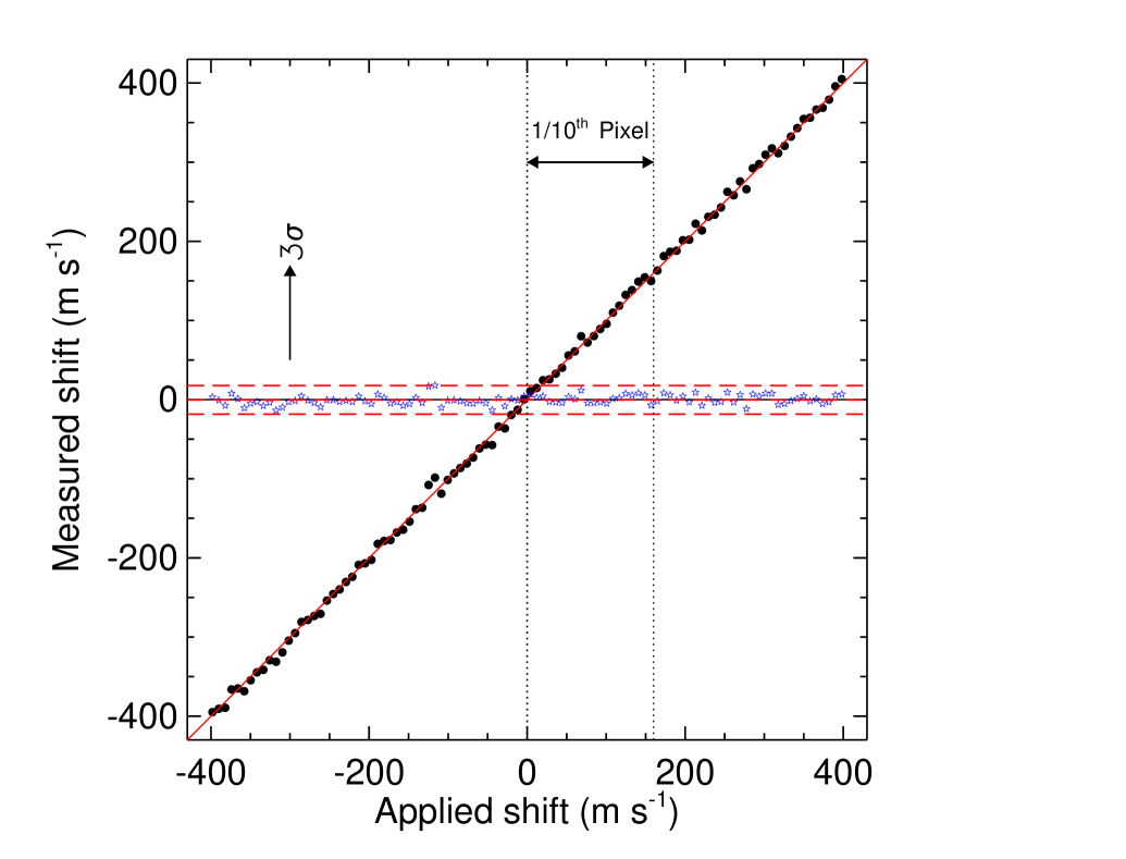
As our cross-correlation analysis implements a rebinning of the spectra on scales of 1/20 of a pixel size and involves very fine interpolations it should be tested against the possible systematics introduced. To check the accuracy of our cross-correlation analysis we carried out a Monte Carlo simulation as follows: (1) generate 90 realizations of the combined spectrum in the range of 3750 3780, with a SNR roughly one fifth of the combined spectrum to mimic the individual exposures, (2) randomly excluding 25–35 pixels from the realized spectrum to mimic the cosmic ray rejected pixels, (3) applying the same velocity shift to all the 90 realizations and (4) cross-correlating the combined spectrum with each of the 90 spectra to measure the shifts. The filled circles in Fig. 1 show the mean measured shifts from 90 realizations vs the applied shifts for a sample of 100 given shifts uniformly chosen between -400 to 400 m s-1. The residuals, shown as asterisks, have a standard deviation of 6 m s-1 and are randomly distributed around the mean of 0 m s-1. The dashed vertical lines in Fig. 1 show the scale of one-tenth of our pixel size. The exercise demonstrates that our method works very well in detecting the sub-pixel shifts between the combined spectra and the individual spectrum.
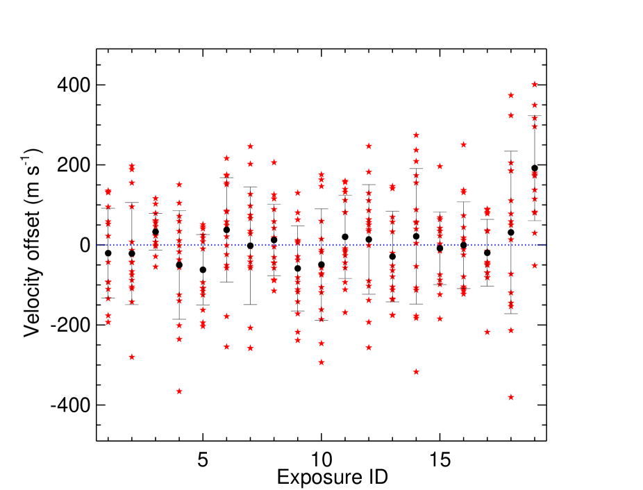
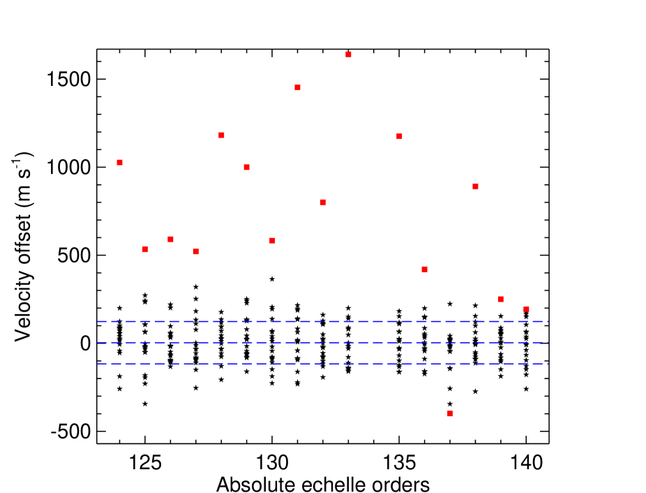
In Fig. 2 we present the measured velocity offset between the combined spectrum and the individual exposures in m s-1 over small wavelength ranges (of size typical of one echelle order). The weighted mean and standard deviation of velocities for each exposure are shown as filled circle and error bar. Apart from exposure 19 (EXP19) all the spectra seem to have average shifts of less than 100 m s-1. In the case of EXP19 the average shift is 195 m s-1. In addition, only one wavelength window has a negative shift and the rest have positive shifts. Therefore, this exposure seems to be severely affected by some systematics. Having a reasonably high SNR, this exposure has already transformed this systematic error to the combined spectrum leading to a erroneous shift estimation. To have a correct estimate of the velocity offsets we make a combined spectrum after excluding EXP19 and repeat the cross-correlation analysis. Fig. 3 presents the amplitude of the velocity offset in m s-1 in different windows for all of the exposures measured with respect to the combined spectrum excluding EXP19. The velocity offsets corresponding to the EXP19 are shown as filled squares. These points have a mean value of 740 m s-1. There also exists a mild trend for the measured shifts of EXP19 to be larger in the red (smaller echelle orders) compared to the blue part (larger echelle orders). We confirm the large velocity shifts in EXP19 using two independent data reductions.
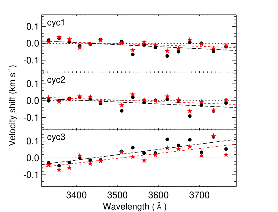
The three cycles of quasar observations are separated by gaps of approximately one year. We next cross-correlate the combined spectrum with that of each cycle to check the stability of the UVES during our observations. The filled circles in different panels of Fig. 4 present the results of this analysis for each cycle. While velocity offsets of the first two cycles show a weak decreasing trend (top two panels of Fig. 4) with increasing wavelength the last cycle data shows a more pronounced trend of velocity offset increasing with increasing wavelength. The filled asterisks in Fig. 4 show the result of similar analysis but after excluding EXP19 both in the total combined spectrum and the combined spectrum of the third cycle. A careful comparison of the asterisks and circles in the first two cycles shows that for Å all asterisks have larger values while for Å they do match. The wavelength dependent trend in the last cycle has been weakened a bit but still persists even after removing the contribution of EXP19 to the combined spectrum. The exercise shows that in addition to a constant shift there could be a wavelength dependent drift in EXP19. Further we also see the indication that even other exposures taken in cycle-3 may have some systematic shift with respect to those observed in previous 2 cycles. Such trends if real should then be seen in the UVES spectra of the other objects observed in 2012. Probing this will require bright objects where high SNR spectrum can be obtained with short exposure times. Asteroids have been frequently observed with UVES during different cycles and they provide a unique tool for this purpose. We test our prediction about UVES using asteroids in section 3.2.
3.2 Analysis of the asteroids spectra observed with UVES
The cross-correlation analysis presented above allowed us to detect the regions and/or exposures that have large velocity offsets in comparison to the combined spectrum. However, this exercise is mainly sensitive to detect relative shifts. One needs an absolute wavelength reference with very high accuracy for investigating any absolute wavelength drift in the UVES spectrum. Moreover, the low SNR of the individual spectra in the wavelength range of 3600 Å does not allow for the direct one-to-one comparison between different individual exposures. As a result an accurate understanding of the possible UVES systematics requires some other absolute references and/or spectra of bright objects. Asteroids are ideally suited for this kind of analysis (see Molaro et al., 2008) as they are very bright, their radial velocities are known to an accuracy of 1 m s-1, and their spectra are filled with the solar absorption features throughout any spectral range of interest. Several asteroids have been observed with UVES during different observing cycles for the purpose of tracking the possible wavelength calibration issues in UVES. In this section we make use of the spectra of these objects observed with UVES to investigate the possible wavelength dependent velocity shifts during different cycles. To do so we select asteroids that were observed with UVES setting of 390 nm in the BLUE similar to our observations (see Table 1). Table 2 shows the observing log of the asteroids used in our analysis. We reduced these data following the same procedure described in section 2 while using attached mode ThAr lamp for all the exposures.
| Name | Observation | Exposure | Seeing | Airmass | Spectral | Slit width |
|---|---|---|---|---|---|---|
| date | (s) | (arcsec) | resolution | (arcsec) | ||
| IRIS | 19-12-2006 | 300 | 1.21 | 1.50 | 81592 | 0.6 |
| 23-12-2006 | 300 | 1.48 | 1.47 | 82215 | 0.6 | |
| 24-12-2006 | 300 | 1.25 | 1.46 | 81523 | 0.6 | |
| 25-12-2006 | 300 | 1.35 | 1.44 | 81381 | 0.6 | |
| 26-12-2006 | 450 | 1.79 | 1.44 | 81479 | 0.6 | |
| 29-03-2012 | 600 | 1.07 | 1.14 | 59107 | 0.8 | |
| 30-03-2012 | 600 | 1.20 | 1.17 | 59151 | 0.8 | |
| 31-03-2012 | 600 | 1.19 | 1.18 | 58439 | 0.8 | |
| 01-04-2012 | 600 | 0.99 | 1.21 | 58538 | 0.8 | |
| CERES | 31-10-2011 | 180 | 0.99 | 1.07 | 57897 | 0.8 |
| 31-10-2011 | 180 | 0.83 | 1.09 | 57810 | 0.8 | |
| 01-11-2011 | 180 | 1.09 | 1.08 | 62204 | 0.8 | |
| 30-10-2010 | 180 | 1.54 | 1.37 | 60828 | 0.8 | |
| 01-11-2010 | 180 | 1.20 | 1.36 | 60621 | 0.7 | |
| 03-11-2010 | 180 | 0.97 | 1.41 | 60415 | 0.8 | |
| EROS | 27-03-2012 | 600 | 1.14 | 1.12 | 58852 | 0.8 |
| 28-03-2012 | 600 | 1.23 | 1.18 | 58535 | 0.8 | |
| 29-03-2012 | 600 | 1.72 | 1.22 | 58841 | 0.8 | |
| 31-03-2012 | 600 | 0.97 | 1.19 | 57681 | 0.8 |
Table 2 shows that the time gap between different observations can vary from hours to years. This allows us to probe the UVES stability in both short and long terms. We further use the solar spectrum as an absolute reference and compare it with the UVES calibrated spectra of the asteroids.
3.2.1 Asteroid-asteroid comparison
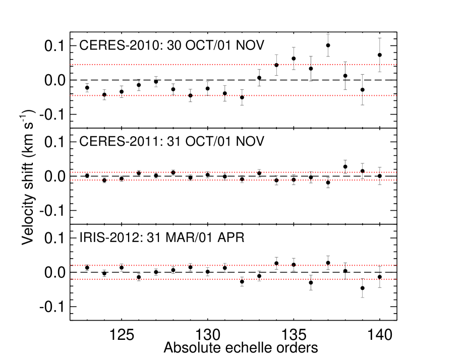
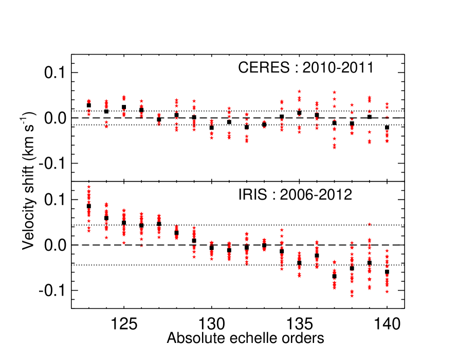
We apply a cross-correlation analysis as described in Section 3.1 to compare asteroid spectra observed at different epochs. Fig. 5 shows the mean subtracted velocity shifts between the asteroids spectra observed with one or two nights of time gap during three different cycles. The abscissa is the absolute echelle order of the UVES and we have only shown the results for the orders that cover the wavelength range of 3330-3800 Å. The velocity offsets hardly reach a peak-to-peak difference of 50 m s-1 in the case of 2011 and 2012 observation. The scatter we notice here is very much similar to the one found by Molaro et al. (2008). The larger velocity errors and scatter seen in the case of 2010 observation is related to the lower SNR of the spectra of these asteroids as they are observed in a high airmass (see Table 2). However, this exercise shows that UVES is stable over short time scales (i.e. a gap of up to 2 days). Fig. 6 shows the velocity offsets between the spectra of IRIS observed in 2006 and 2012 (bottom panel) and spectra of CERES observed in 2010 and 2011 (top panel). Asterisks are used to show the individual velocity offsets seen in each order and the filled squares show the mean of them. While in the case of CERES we find a (random) pattern (within a v = 20 ms-1 ) similar to what we see in Fig. 5, in the case of IRIS there exists a clear steep increase of the mean velocity offsets as one goes towards lower echelle orders (or longer wavelengths). The wavelength dependent velocity shifts seen in the case of IRIS is a signature of a severe systematic effect affecting the UVES spectrum taken in the year 2012 as suggested by our cross-correlation analysis of the quasar spectra (see Fig. 4). As the experiment carried out here is relative we cannot clearly conclude whether the problem comes from either of the cycles or both. However, Molaro et al. (2008) did not find any wavelength dependent systematics while comparing its absorption wavelengths in IRIS spectrum taken in the year 2006 with those of solar spectra for Å. Unraveling this problem requires a very accurate absolute wavelength reference. We will consider the solar spectrum as an absolute reference for this purpose in the next section for further exploring this systematic.
3.2.2 Solar-asteroid comparison
Molaro et al. (2008) have used the very accurate wavelengths of the solar absorption lines in the literature as the absolute reference and compared them with the measured wavelengths of the same lines in the asteroid spectrum observed with UVES. Unfortunately, such an exercise is only possible for 4000 Å as the solar absorption lines are severely blended for shorter wavelengths. However using an accurately calibrated solar spectrum we can cross-correlate it with the asteroid spectra of different years. We use the solar spectra discussed in Kurucz (2005, 2006) as the solar spectrum template222The spectrum is taken from http://kurucz.harvard.edu/sun/fluxatlas2005/. This spectrum is corrected for telluric lines and the wavelength scale of the spectrum is corrected for the gravitational redshift ( 0.63 km s-1) and given in air. Therefore we used UVES spectra before applying air-to-vacuum conversion for the correlation analysis. The uncertainties associated with the absolute wavelength scale of Kurucz (2005) is ms-1. We then measure the velocity offset between the solar and asteroid spectra in windows of the sizes of the UVES orders between 3330 Å to 3800 Å.
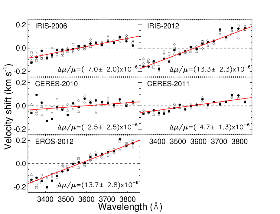
The results of the correlation analysis are presented in Fig. 7 as the solar-asteroid offset velocity vs the wavelength. Different symbols in each panel correspond to different asteroid exposures obtained within a period of couple of days. We have subtracted the mean velocity offset (coming from the radial velocity differences) in each case to bring the mean level to zero. A qualitative inspection shows that the velocity offsets in all cases increase as wavelengths increase though with different slopes for different years. Obviously the two asteroids spectra acquired in 2012 show the largest slopes. As wavelength dependent velocity shifts can mimic a non-zero , it is important to translate the observed trend to an apparent . To estimate what is the effect of such a wavelength dependent systematics in our measurements we carried out the following exercise: (1) First we fit a straight line to the velocity offset vs wavelength to get , (2) finding the offset and at the observed wavelengths of our interested lines and assign a Ki to each , (3) generating 2000 Gaussian realizations of each (or reduced redshift) with the scatter of , (4) a measurements from reduced redshift vs K analysis for each of the 500 realizations, and (5) finding the mean and the scatter of the distribution as the systematic and its error. In Fig. 7 we have shown the estimated for each of the asteroid data. Typical error in is found to be 2.5. The minimum = (2.52.5) is obtained for the case of CERES-2010 observation. Spectra of IRIS-2012 and EROS-2012 show trends that are significant at more that 4.5 level. These trends translates to a of (13.32.3) and (13.72.8) respectively for IRIS-2012 and EROS-2012. This clearly confirms our finding that the UVES data acquired in 2012 has large wavelength drifts. As the amplitude of from the wavelength drift noted above is close to we wish to detect with our lines it is important to remove these systematics from the data. Therefore, in what follows in addition to standard measurements we also present measurements after correcting the redshifts of lines using the relationship found between the velocity offset and wavelength for the asteroid spectrum obtained closest to the quasar observations.
In summary the analysis presented in this section suggests that one of the exposures (EXP19) shows a systematically large shift compared to the rest of the data. Therefore, we exclude this exposure when we discuss our final combined data to measure . Our analysis also suggests the existence of wavelength dependent velocity shift in particular in the spectra acquired in year 2012. Therefore, we present our results for combined data of only first two cycles of data to gauge the influence of wavelength dependence drift in the data acquired in 2012.
4 Constraints on
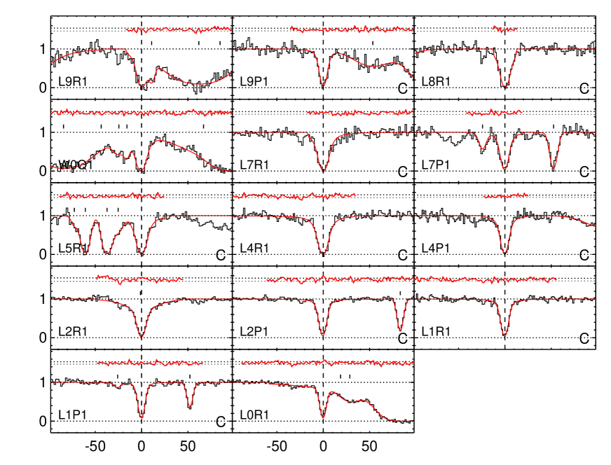
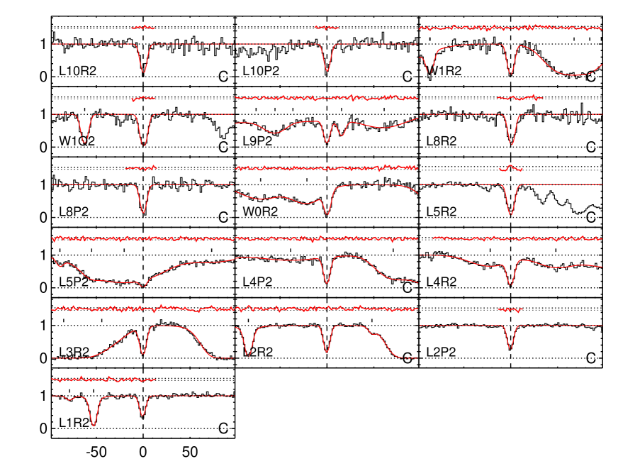
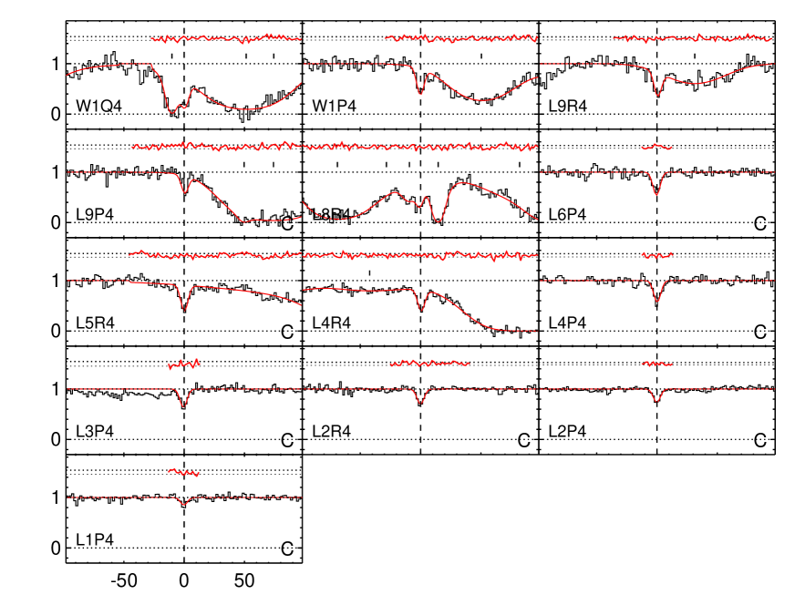
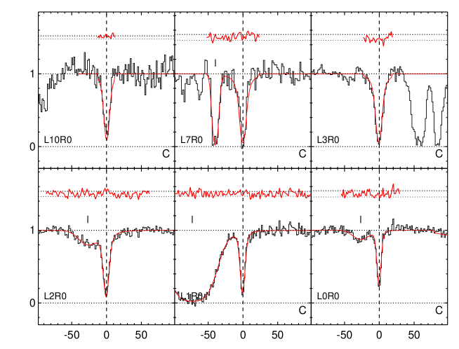
The 2.4018 DLA towards HE 00271836 produces more than 100 absorption lines in the observed wavelength range of 3330 Å to 3800 Å (see Figs. 19 – 25 in Noterdaeme et al., 2007). These are from different rotational states spanning from 0 to 6. While we detect a couple of transitions of 6 in absorption, they are too weak to lead to any reasonable estimation of the absorption line parameters (in particular the accurate value of ) of this level. Therefore, we do not make use of them for constraining . For each rotational level we detect several absorption lines arising from transitions having wide range of oscillator strengths. This makes it possible to have very reliable estimation of fitting parameters and associated errors in our Voigt profile analysis of lines. From all the detected absorption we select 71 useful lines for constraining , out of which 24 may have a mild contamination in the wings from other unrelated absorption features. These mildly contaminated lines are also included in the analysis as their line centroids are well defined and the additional contaminations can be modeled accurately through multiple-component Voigt-profile fitting. lines used in the current study and results of the single component fit are presented in Tables 8 and 9.
Noterdaeme et al. (2007), have found that the width of high lines are systematically broader than that of low lines when a single Voigt profile component was used. As our combined spectrum has a better SNR and pixel sampling compared to that used in Noterdaeme et al. (2007), we revisit the Voigt profile fitting, using vpfit333http://www.ast.cam.ac.uk/ rfc/vpfit.html, before measuring . First we fit all the identified transitions considering single and for all the levels and with the column density being different for different -levels. Our best fitted model has a reduced of 1.421. The best fitted value of the -parameter is 2.100.04 km s-1. In addition, the derived column densities suggest an ortho-to-para ratio (OPR; see Eq. 1 of Srianand et al., 2005, for the definition) of 11.551.42, while is expected in a normal local thermal equilibrium (LTE) conditions. Next we tried the fit very similar to that of Noterdaeme et al. (2007), where we have allowed the parameter to be different for different -levels. In this case the best fit is obtained with a reduced of 1.190 and we notice that the OPR is 2.260.15 as expected in the cold interstellar medium. Most of the total H2 column density in this system is contributed by = 0 and = 1 levels. The best fitted -parameters are 0.890.05 km s-1 and 1.400.04 km s-1 respectively for = 0 and = 1 levels. The abnormal values of OPR obtained when we fix to be same for all -levels can be attributed to the line saturation and the average being much higher than the best fitted values of = 0 and = 1. This exercise, confirms the finding of Noterdaeme et al. (2007) that the absorption profile of high--levels are broader than that of the low- ones. This is one of the models we use in our analysis to find the best fitted value of . As pointed out by Noterdaeme et al. (2007), observed differences in the excitation temperatures and velocity width of high and low -levels may point towards multiphase nature of the absorbing gas. In order to take this into account we allow for the mean redshift of absorption from different levels to be different in our analysis.
Alternatively, one could model the two phase nature of the absorbing gas by using two component Voigt profile fits. In this case we constrain and of the two components to be the same for different -levels and perform Voigt profile fits. Our best fit model has a reduced of 1.192 with two components having = 0.940.04 km s-1 and = 1.890.3 km s-1and velocity separation of 4.40.2 km s-1. This reduced is very similar to what we found for the single component fit with different values for different -levels discussed above. The first component at contains 99% of the total column density and has an OPR of 2.270.13. The second weaker component has an OPR of 3.070.42. We further model the lines with two components while allowing different -levels to have different values. In this model is constrained to be same for all -levels. The best fitted model in such a case has a reduced of 1.177 with two components having a velocity separation of 4.00.4 km s-1. The reduced is slightly improved in comparison with the case where was tied. The first component at contains more than 99% of the total column density and has an OPR of 2.110.16. The second weaker component has an OPR of 2.920.57. Unlike the previous 2-component model, here both components have OPR consistent with what is expected under the LTE conditions. We consider this two component model as the second case while measuring the value from our data.
There are two approaches used in literature to measure using absorption lines: (i) linear regression analysis of vs with as the slope (see for example Varshalovich & Levshakov, 1993; Ivanchik et al., 2005; Reinhold et al., 2006; Wendt & Molaro, 2011) or (ii) use as an additional parameter in the vpfit programme (see for example King et al., 2008; Malec et al., 2010; King et al., 2011). We employ both the methods to derive from our data considering two cases: (i) single component Voigt profile fit (called case-A) and (ii) two component fit (called case-B).
4.1 Statistical errors from vpfit
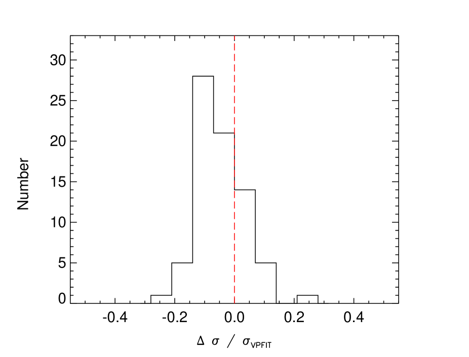
The vpfit program estimates errors in each parameter only using the diagonal terms of the covariance matrix. These are reliable in cases where the lines are not strongly contaminated and are resolved out of the instrumental resolution. Measured parameters of the lines detected towards HE 00271836, especially those from = 0 and = 1 levels, are several times smaller than the instrumental resolution which is 5.0 km s-1 (see Table 3). In such cases the reliability of the vpfit errors should be investigated (see Carswell et al., 2011). To do so we generate 100 simulated spectra with a same SNR as the final combined spectrum. For this we consider our best fitted single component Voigt profile model obtained by vpfit and add Gaussian noise to achieve the same SNR as the original spectrum. We then fit the lines of each mock spectrum using the same fitting regions and initial guess parameters as those used in case of our best fit model. Finally for each of the transitions we compare the 1 distribution from the 100 mock redshifts with the estimated error from vpfit. Fig. 8 shows the distribution of the relative error differences of redshifts, (i.e. () of all the lines used in this analysis. Clearly when we use majority of the transitions vpfit does not underestimate the redshift errors. As it can be seen from this histogram the two errors are always consistent and in 73% of cases vpfit predicts a higher value for the error. We confirm that the same result holds for errors associated with N and parameters obtained from the vpfit. We repeated the analysis for the two component fit as well and found that the error obtained from the vpfit adequately represents the statistical error of the parameters. Therefore we will only use the vpfit errors as statistical errors in redshifts.
4.2 measurements using -vs- analysis
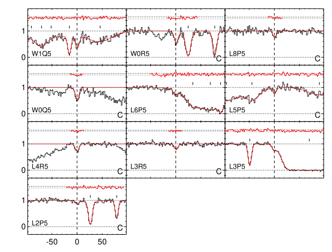
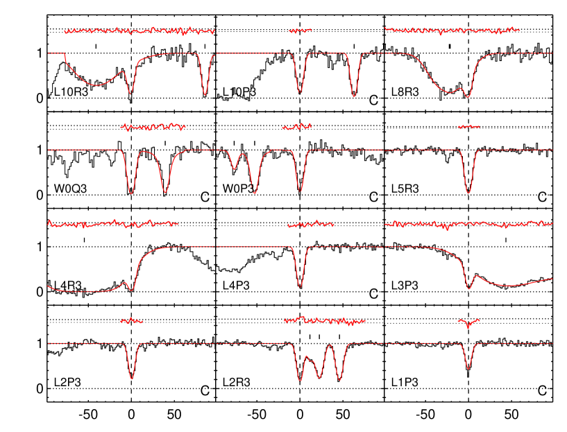
Following previous studies (Ivanchik et al., 2005; Reinhold et al., 2006; Ubachs et al., 2007; Wendt & Molaro, 2011, 2012) we carry out measurements based on the -vs- linear regression analysis in this section. We use the redshifts of individual transitions obtained from the vpfit for case-A discussed above. Fig. 13 shows our best fitted Voigt profile for = 3 transitions for the combined spectrum made of all exposures excluding EXP19. transitions L1P3, L2P3, L4P3, L5R3, W0Q3, and L10P3 are the examples of what we classify as CLEAN lines. The rest of the absorption lines shown in Fig. 13 are classified as blended. Voigt profile fits to these lines are performed by suitably taking care of the blending. Fits to lines from other -levels are shown in Appendix C. The fitting results for lines used in measurements are presented in Appendix B. Table 3 summarizes the column density, parameter, and the mean redshift for each -level. As -level increases the velocity offset with respect to = 0 and the parameter of the corresponding level also increases. The only exception is = 4 that its velocity offset and parameter are less than those of = 3 but still larger than = 2.
| -level | N | log[N(J)] | ||||
|---|---|---|---|---|---|---|
| km s-1 | km s-1 | log[cm-2] | km s-1 | |||
| (1) | (2) | (3) | (4) | (5) | (6) | (7) |
| 0 | 6 | 2.4018452 | 0.07 | 0.00 | 16.910.02 | 0.900.06 |
| 1 | 14 | 2.4018486 | 0.05 | 0.30 | 17.270.02 | 1.410.04 |
| 2 | 16 | 2.4018499 | 0.07 | 0.41 | 14.950.02 | 2.680.07 |
| 3 | 12 | 2.4018522 | 0.08 | 0.62 | 15.000.02 | 3.340.14 |
| 4 | 13 | 2.4018513 | 0.11 | 0.54 | 14.190.02 | 2.550.38 |
| 5 | 10 | 2.4018550 | 0.15 | 0.87 | 13.910.02 | 3.890.31 |
Column (1): indices for different rotational levels. Column (2): number of transitions in the given -level Column (3): mean weighted redshift of all transitions having same -level. Column (4): redshift error in km s-1. Column (5): redshift difference between the given -level and in km s-1. Column (6): The log of the column density for different -levels in cm-2. Column (7): parameter in km s-1for different -levels
In our linear regression analysis we do not use the redshift errors from vpfit as our analysis in section 3.2 shows that the wavelengths of different regions may be affected by some systematic error. As this error is independent of the statistical redshift error it makes the distribution of the redshift to have a larger scatter than that allowed by the statistical error we get from the Voigt profile fitting. Therefore, we use a bootstrap technique for estimating the realistic error of our regression analysis. To do so we generate 2000 random realizations of the measured redshifts and estimate for each of these realization. We finally quote the 1 scatter of the 2000 as the estimated error in . From Table 3 we can see that the mean redshifts of different -levels may be different in this case. Therefore in our analysis we allow for the redshifts of different to be different by allowing the intercept in -vs- plot to be different for different -levels.
| z-vs-K | vpfit | |||||||||||
|---|---|---|---|---|---|---|---|---|---|---|---|---|
| 1-component | 1-component | 2-components | ||||||||||
| (1) | (2) | (3) | (4) | (5) | (6) | (7) | (8) | (9) | (10) | (11) | (12) | (13) |
| cycle | original | corrected† | original | AICC | corrected† | original | AICC | corrected† | ||||
| 1 | 1.7 16.3 | 4.6 16.8 | 21.110.0 | 1.037 | 6302 | 19.8 9.9 | 1.029 | 11.712.2 | 1.032 | 6295 | 12.111.8 | 1.022 |
| 2 | 30.212.2 | 26.712.7 | 15.510.5 | 0.974 | 5948 | 10.010.5 | 0.972 | 10.711.9 | 0.969 | 5936 | 5.2 11.9 | 0.967 |
| 3⋆ | 41.619.5 | 30.119.0 | 30.214.3 | 0.932 | 5705 | 14.512.5 | 0.927 | 12.913.5 | 0.912 | 5614 | 0.8 13.4 | 0.907 |
| 1+2 | 10.711.4 | 13.810.2 | 18.8 7.7 | 1.128 | 6825 | 15.8 7.7 | 1.123 | 0.8 8.6 | 1.120 | 6794 | 1.5 8.7 | 1.115 |
| 1+2+3⋆ | 20.0 9.3 | 15.09.3 | 21.8 6.9 | 1.188 | 7167 | 15.6 6.9 | 1.179 | 2.5 8.1 | 1.178 | 7115 | 7.6 8.1 | 1.171 |
⋆ result of the cases that EXP19 is excluded.
† results after correcting the systematics based on the solar-asteroid cross-correlation.
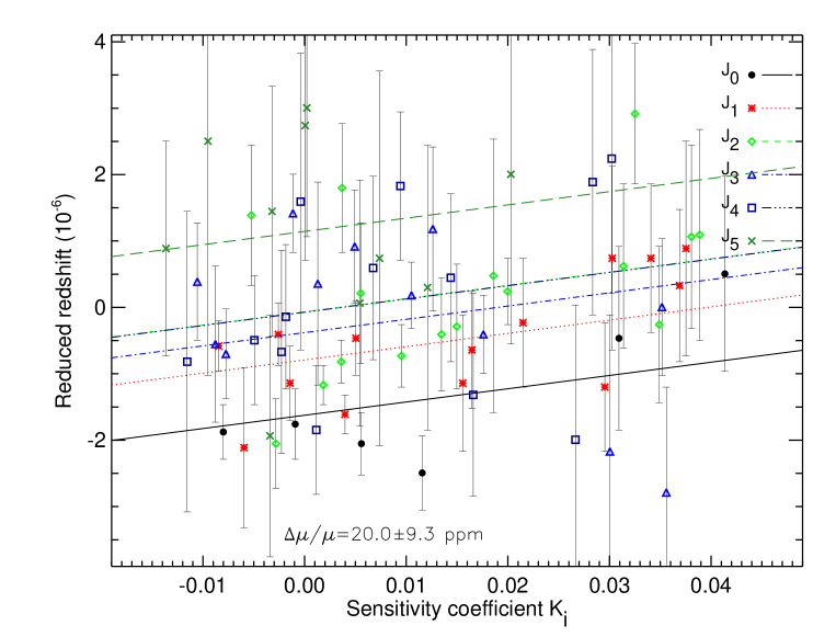
In Fig. 10 we plot the reduced redshift vs for different transitions. The points from different -levels are marked with different symbols. The best fitted line for points from different -levels are also shown in the figure with different line styles. As discussed before, we constrained the slope (i.e. ) of these lines to be same while allowing for the intercept (i.e. mean redshift) to be different for different -levels. The best fitted value for is ppm (See column 2 of the last row in Table 4). The quoted error is obtained using bootstrapping as discussed above.
As the wavelength dependent velocity shift is found to be minimum in the case of first two cycles we measured the using only the data obtained in the first two cycles (i.e. 13 exposures and total integration time of hrs). We call this sub-sample as “1+2”. The results of the measurement for this case is also given in Table. 4. We find = 10.711.4 ppm. As expected the mean obtained from this sub-sample is less than the one obtained for the whole sample. The amount of observing time in different cycles are respectively 10.4 hours, 12.5 hours, and 10.4 hours for the first, second, and third cycle. Therefore, we also measured using data obtained in individual cycles. The total observing time in each cycle is sufficiently good for estimating based on each cycle. We get = ppm, ppm and ppm respectively for the first, second and third cycles. The progressive increase in the mean is consistent with what we notice in Fig. 7 for the asteroids.
The final combined spectrum used here is based on 18 exposures. With such a large number of exposures, in principle the result of our analysis should not be sensitive to individual exposures. To test this we make 100 combined spectra of 15 randomly chosen individual exposures and measure using -vs- analysis of single component fit (case-A) as discussed above for the full sample. Fig. 11 shows the distribution of the measured . The mean we measure (i.e. ) is consistent with the mean we get for the full sample. The 1 scatter around the mean is 3.6. As expected this is much smaller than the statistical error in individual measurements.
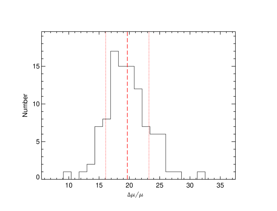
Thus we feel that the bootstrap method adequately quantifies the errors in our measurements.
Now we will apply corrections to the velocity drift seen in the case of asteroids to the individual spectrum and see its effect in the measurements. To do so we first shift the observed wavelength of each pixel of each individual exposure based on the modeled velocity offsets obtained from the solar-asteroid cross-correlation analysis in the corresponding observing cycle. We then combine these shifted individual spectra to make the final combined spectrum. Only in Cycle 2 we have asteroid observations taken on the same nights of the quasar observation. In the other two cycles the nearest asteroid observations are obtained within 3.5 months to the quasar observations. While this is not the ideal situation this is the best we can do. Results of measurements after applying the drift correction for different cases are summarized in column 3 of Table 4. The results of after applying drift corrections are summarized in column 4 of Table 4. We find = ppm for the combined data after applying corrections. Clearly an offset at the level of 5 ppm comes from this effect alone in the combined data. We wish to note that the estimated after applying corrections should be considered as an indicative value as we do not have asteroid observations on the same nights of quasar observations. In addition the quasar and asteroid observations are very different in terms of the exposure times and the source angular size.
We notice that because of severe blending, -vs- method cannot be easily applied to the two component fit (case-B). In the following section we obtain directly from vpfit for both single and two component fits.
4.3 measurements using vpfit
We performed the Voigt profile fitting of all the chosen lines keeping as an additional fitting parameter. The results are also summarized in columns 4 – 13 in Table 4. When we consider the single component fit (case-A) we find = ppm for the full sample with a reduced of 1.188 (see columns 4 and 5 in Table 4). This is very much consistent with what we have found above using -vs- analysis. We find the final value to be robust using different input parameter sets. When we fit the data obtained from first two cycles we find = ppm with a reduced of 1.128. This also confirms our finding that the addition of third year data increases the measured mean of . Table 4 also summarizes the results of measurements for data taken on individual cycles. When we use the corrected spectrum for the full sample we get = ppm. The measurements for different cases after applying the correction and the corresponding reduced are given in columns 7 and 8 respectively. As noted earlier the statistical errors from the vpfit are about 25 to 30% underestimated compared to the bootstrap errors obtained in the -vs- analysis. It is also clear from the table that correcting the velocity offset leads to the reduction of the up to 6.2 ppm for the combined dataset. Column 6 in Table 4 gives the Akaike information criteria (AIC; Akaike, 1974) corrected for the finite sample size (AICC; Sugiura, 1978) as given in the Eq. 4 of King et al. (2011). We can use AICC in addition to the reduced to discriminate between the models.
Next we consider the two component Voigt profile fits (i.e. case-B) where we keep as an additional fitting parameter. The results are also summarized in columns 9 – 13 of Table 4. The measurements, associated reduced and AICC parameters for uncorrected data are given in columns 9, 10 and 11 respectively. Results for the corrected data are provided in columns 12 and 13. For the whole sample we find = ppm with a reduced of 1.177. The reduced in this case is slightly lower than the corresponding single component fit. In addition we find the difference in AICC is 52 in favour of two component fit (i.e. case B). Table 4 also presents results for individual cycle data for the two components fit.
The comparison of AICC given in columns 6 and 11 of the Table 4 also clearly favours the two component fit (i.e. case-B). Therefore, we will only consider measurements based on two component fit in the following discussions. However, bootstrapping errors in the case of -vs- linear regression analysis (of single component fit) are larger and robust when comparing with the errors from vpfit. In the case of combined spectrum of all exposures (last row of Table 4) we need to quadratically add 6.2 ppm to the vpfit error to get the -vs- error. This can be considered as typical contribution of the systematic errors. So we consider the two component fit results with the enhanced error in further discussions.
5 Discussion
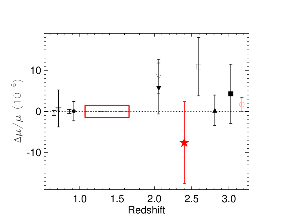
We have analyzed the absorption lines from a DLA at = 2.4018 towards HE 00271836 observed with VLT/UVES as part of the ESO Large Programme ”The UVES large programme for testing fundamental physics”. We carried out measurements based on -vs- analysis. Our cross-correlation analysis shows that one of the exposures has a large velocity shift with respect to the remaining exposures. Excluding this exposure from the combined spectrum we find a = .
To understand the possible systematics affecting our observations we studied the asteroids observed with VLT/UVES in different cycles. Comparing the asteroids spectra and very accurate solar spectrum we show the existence of a wavelength dependent velocity shift with varying magnitude in different cycles. Correcting our observations for these systematics we measure = . Our measurement is consistent with no variation in over the last 10.8 Gyr at a level of one part in 105. Our null result is consistent with measurements in literature from analysis of different -bearing sightlines (Thompson et al., 2009a, Table 1).
Fig. 12 summarizes the measurements based on different approaches at different redshifts. As can be seen our new measurement is also consistent with the more recent accurate measurements using at . Wendt & Molaro (2012) found a = using the absorber at = 3.025 towards Q0347383. King et al. (2011) and van Weerdenburg et al. (2011) used and HD absorbers at respectively = 2.811 and 2.059 towards Q0528250 and J2123005 to find = and = . The measurement towards Q0528250 is the most stringent measurements reported till date. However, large discrepancies (a factor of 50) in the reported N() values by King et al. (2011) and Noterdaeme et al. (2008) is a concern and its effect on needs to be investigated. King et al. (2008) have found = at = 2.595 towards Q0405443. Using these measurements and ours we find the weighted mean of = . If we use the measurement of Thompson et al. (2009a) of = for the system towards Q0405443 we get the mean value of = . However we wish to point out that three out of four UVES based measurements show positive values of . As any wavelength dependent drift in these cases could bias these measurements towards positive (See Section 3.2.2) we should exercise caution in quoting combined measurements.
Best constraints on in quasar spectra are obtained using either NH3 or CH3OH (Murphy et al., 2008; Henkel et al., 2009; Kanekar, 2011; Bagdonaite et al., 2013). These measurements reach a sensitivity of in . However, only two systems at high redshift are used for these measurements and both at 1. Based on 21-cm absorption we have = (at 1.3 by Rahmani et al., 2012) and = (at 3.2 by Srianand et al., 2010). While these measurements are more stringent than based measurements one has to assume no variation in and to get a constraint on . Also care needs to be taken to minimize the systematics related to the line of sight to radio and optical emission being different.
acknowledgement
R. S. and P. P. J. gratefully acknowledge support from the Indo-French Centre for the Promotion of Advanced Research (Centre Franco-Indian pour la Promotion de la Recherche Avancée) under contract No. 4304-2. P.M. and C.J.M. acknowledge the financial support of grant PTDC/FIS/111725/2009 from FCT (Portugal). C.J.M. is also supported by an FCT Research Professorship, contract reference IF/00064/2012. The work of S.A.L. is supported by DFG Sonderforschungsbereich SFB 676 Teilprojekt C4. M.T.M. thanks the Australian Research Council for Discovery Project grant DP110100866 which supported this work.
References
- Agafonova et al. (2013) Agafonova, I. I., Levshakov, S. A., Reimers, D., Hagen, H.-J., & Tytler, D., 2013, A&A, 552, A83
- Agafonova et al. (2011) Agafonova, I. I., Molaro, P., Levshakov, S. A., & Hou, J. L., 2011, A&A, 529, A28+
- Akaike (1974) Akaike, A., 1974, IEEE Trans. Autom. Control, 19, 716
- Amendola et al. (2012) Amendola, L., Leite, A. C. O., Martins, C. J. A. P., Nunes, N. J., Pedrosa, P. O. J., & Seganti, A., 2012, Phys. Rev. D, 86, 063515
- Bagdonaite et al. (2013) Bagdonaite, J., Jansen, P., Henkel, C., Bethlem, H. L., Menten, K. M., & Ubachs, W., 2013, Science, 339, 46
- Bailly et al. (2010) Bailly, D., Salumbides, E. J., Vervloet, M., & Ubachs, W., 2010, Molecular Physics, 108, 827
- Carswell et al. (2011) Carswell, R. F., Jorgenson, R. A., Wolfe, A. M., & Murphy, M. T., 2011, MNRAS, 411, 2319
- Chand et al. (2006) Chand, H., Srianand, R., Petitjean, P., Aracil, B., Quast, R., & Reimers, D., 2006, A&A, 451, 45
- Cowie & Songaila (1995) Cowie, L. L. & Songaila, A., 1995, ApJ, 453, 596
- Dekker et al. (2000) Dekker, H., D’Odorico, S., Kaufer, A., Delabre, B., & Kotzlowski, H., 2000, in Proc. SPIE Vol. 4008, p. 534-545, Optical and IR Telescope Instrumentation and Detectors, Masanori Iye; Alan F. Moorwood; Eds., pp. 534–545
- D’Odorico et al. (2000) D’Odorico, S., Cristiani, S., Dekker, H., Hill, V., Kaufer, A., Kim, T., & Primas, F., 2000, in Society of Photo-Optical Instrumentation Engineers (SPIE) Conference Series, Vol. 4005, Society of Photo-Optical Instrumentation Engineers (SPIE) Conference Series, J. Bergeron, ed., pp. 121–130
- Edlén (1966) Edlén, B., 1966, Metrologia, 2, 71
- Ferreira et al. (2012) Ferreira, M. C., Julião, M. D., Martins, C. J. A. P., & Monteiro, A. M. R. V. L., 2012, Phys. Rev. D, 86, 125025
- Henkel et al. (2009) Henkel, C., Menten, K. M., Murphy, M. T., et al., 2009, A&A, 500, 725
- Ivanchik et al. (2005) Ivanchik, A., Petitjean, P., Varshalovich, D., Aracil, B., Srianand, R., Chand, H., Ledoux, C., & Boissé, P., 2005, A&A, 440, 45
- Jorgenson et al. (2013) Jorgenson, R. A., Murphy, M. T., Thompson, R., & Carswell, R. F., 2013, submitted to MNRAS
- Kanekar (2011) Kanekar, N., 2011, ApJ, 728, L12
- King et al. (2011) King, J. A., Murphy, M. T., Ubachs, W., & Webb, J. K., 2011, MNRAS, 417, 3010
- King et al. (2008) King, J. A., Webb, J. K., Murphy, M. T., & Carswell, R. F., 2008, Physical Review Letters, 101, 251304
- Kozlov & Levshakov (2013) Kozlov, M. G. & Levshakov, S. A., 2013, Annalen der Physik, in press (arXiv: physics.atom-ph/1304.4510)
- Kurucz (2005) Kurucz, R. L., 2005, Memorie della Societa Astronomica Italiana Supplementi, 8, 189
- Kurucz (2006) —, 2006, ArXiv:astro-ph/0605029
- Ledoux et al. (2003) Ledoux, C., Petitjean, P., & Srianand, R., 2003, MNRAS, 346, 209
- Levshakov et al. (2006) Levshakov, S. A., Centurión, M., Molaro, P., D’Odorico, S., Reimers, D., Quast, R., & Pollmann, M., 2006, A&A, 449, 879
- Levshakov et al. (2012) Levshakov, S. A., Combes, F., Boone, F., Agafonova, I. I., Reimers, D., & Kozlov, M. G., 2012, A&A, 540, L9
- Levshakov et al. (2002) Levshakov, S. A., Dessauges-Zavadsky, M., D’Odorico, S., & Molaro, P., 2002, MNRAS, 333, 373
- MacAlpine & Feldman (1982) MacAlpine, G. M. & Feldman, F. R., 1982, ApJ, 261, 412
- Malec et al. (2010) Malec, A. L., Buning, R., Murphy, M. T., et al., 2010, MNRAS, 403, 1541
- Molaro et al. (2013) Molaro, P., Centurión, M., Whitmore, J. B., et al., 2013, A&A, 555, A68
- Molaro et al. (2008) Molaro, P., Levshakov, S. A., Monai, S., Centurión, M., Bonifacio, P., D’Odorico, S., & Monaco, L., 2008, A&A, 481, 559
- Murphy et al. (2008) Murphy, M. T., Flambaum, V. V., Muller, S., & Henkel, C., 2008, Science, 320, 1611
- Noterdaeme et al. (2007) Noterdaeme, P., Ledoux, C., Petitjean, P., Le Petit, F., Srianand, R., & Smette, A., 2007, A&A, 474, 393
- Noterdaeme et al. (2008) Noterdaeme, P., Ledoux, C., Petitjean, P., & Srianand, R., 2008, A&A, 481, 327
- Olive & Skillman (2004) Olive, K. & Skillman, E., 2004, Astrophys. J., 617, 29
- Petitjean et al. (2009) Petitjean, P., Srianand, R., Chand, H., Ivanchik, A., Noterdaeme, P., & Gupta, N., 2009, Space Science Reviews, 35
- Petitjean et al. (2000) Petitjean, P., Srianand, R., & Ledoux, C., 2000, A&A, 364, L26
- Petrov et al. (2006) Petrov, Y., Nazarov, A., Onegin, M., Petrov, V., & Sakhnovsky, E., 2006, Phys. Rev. C, 74
- Rahmani et al. (2012) Rahmani, H., Srianand, R., Gupta, N., Petitjean, P., Noterdaeme, P., & Vásquez, D. A., 2012, MNRAS, 425, 556
- Reinhold et al. (2006) Reinhold, E., Buning, R., Hollenstein, U., Ivanchik, A., Petitjean, P., & Ubachs, W., 2006, Phys. Rev. Lett., 96, 151101
- Rosenband et al. (2008) Rosenband, T., Hume, D., Schmidt, P., et al., 2008, Science, 319, 1808
- Shelkovnikov et al. (2008) Shelkovnikov, A., Butcher, R. J., Chardonnet, C., & Amy-Klein, A., 2008, Phys. Rev. Lett., 100, 150801
- Srianand et al. (2010) Srianand, R., Gupta, N., Petitjean, P., Noterdaeme, P., & Ledoux, C., 2010, MNRAS, 405, 1888
- Srianand et al. (2012) Srianand, R., Gupta, N., Petitjean, P., Noterdaeme, P., Ledoux, C., Salter, C. J., & Saikia, D. J., 2012, MNRAS, 421, 651
- Srianand et al. (2005) Srianand, R., Petitjean, P., Ledoux, C., Ferland, G., & Shaw, G., 2005, MNRAS, 362, 549
- Sugiura (1978) Sugiura, N., 1978, Commun. Stat. A-Theor., 7, 13
- Thompson (1975) Thompson, R. I., 1975, Astrophys. Lett., 16, 3
- Thompson et al. (2009a) Thompson, R. I., Bechtold, J., Black, J. H., et al., 2009a, ApJ, 703, 1648
- Thompson et al. (2009b) Thompson, R. I., Bechtold, J., Black, J. H., & Martins, C. J. A. P., 2009b, New A, 14, 379
- Tzanavaris et al. (2007) Tzanavaris, P., Murphy, M. T., Webb, J. K., Flambaum, V. V., & Curran, S. J., 2007, MNRAS, 374, 634
- Ubachs et al. (2007) Ubachs, W., Buning, R., Eikema, K. S. E., & Reinhold, E., 2007, Journal of Molecular Spectroscopy, 241, 155
- Uzan (2011) Uzan, J.-P., 2011, Living Reviews in Relativity, 14, 2
- van Weerdenburg et al. (2011) van Weerdenburg, F., Murphy, M. T., Malec, A. L., Kaper, L., & Ubachs, W., 2011, Physical Review Letters, 106, 180802
- Varshalovich & Levshakov (1993) Varshalovich, D. A. & Levshakov, S. A., 1993, Soviet Journal of Experimental and Theoretical Physics Letters, 58, 237
- Wendt & Molaro (2011) Wendt, M. & Molaro, P., 2011, A&A, 526, A96+
- Wendt & Molaro (2012) —, 2012, A&A, 541, A69
- Whitmore et al. (2010) Whitmore, J. B., Murphy, M. T., & Griest, K., 2010, ApJ, 723, 89
Appendix A Results of correlation analysis
| regions | EXP01 | EXP02 | EXP03 | EXP04 | EXP05 | EXP06 |
|---|---|---|---|---|---|---|
| (km s-1) | (km s-1) | (km s-1) | (km s-1) | (km s-1) | (km s-1) | |
| 33193345 | 0.13 0.20 | 0.16 0.18 | 0.00 0.09 | 0.06 0.12 | 0.05 0.12 | 0.16 0.19 |
| 33453370 | 0.05 0.15 | 0.01 0.13 | 0.06 0.07 | 0.05 0.13 | 0.05 0.12 | 0.05 0.16 |
| 33703395 | 0.13 0.17 | 0.19 0.15 | 0.00 0.07 | 0.06 0.12 | 0.01 0.11 | 0.02 0.16 |
| 33953421 | 0.04 0.15 | 0.11 0.15 | 0.02 0.07 | 0.07 0.15 | 0.02 0.11 | 0.25 0.16 |
| 34213446 | 0.10 0.15 | 0.07 0.16 | 0.03 0.07 | 0.01 0.13 | 0.06 0.10 | 0.02 0.17 |
| 34463472 | 0.13 0.14 | 0.10 0.17 | 0.02 0.08 | 0.00 0.15 | 0.02 0.10 | 0.06 0.19 |
| 34983523 | 0.02 0.16 | 0.20 0.16 | 0.06 0.10 | 0.10 0.15 | 0.11 0.11 | 0.18 0.17 |
| 35233552 | 0.18 0.12 | 0.04 0.15 | 0.08 0.09 | 0.24 0.12 | 0.12 0.10 | 0.06 0.14 |
| 35523578 | 0.02 0.14 | 0.28 0.16 | 0.01 0.08 | 0.15 0.14 | 0.11 0.12 | 0.17 0.19 |
| 35783607 | 0.09 0.14 | 0.07 0.13 | 0.01 0.07 | 0.20 0.15 | 0.04 0.10 | 0.08 0.17 |
| 36073636 | 0.09 0.12 | 0.14 0.14 | 0.05 0.08 | 0.12 0.11 | 0.20 0.09 | 0.00 0.13 |
| 36363662 | 0.19 0.15 | 0.04 0.15 | 0.05 0.10 | 0.03 0.16 | 0.09 0.13 | 0.15 0.17 |
| 36623691 | 0.11 0.10 | 0.01 0.10 | 0.12 0.06 | 0.04 0.09 | 0.16 0.08 | 0.18 0.12 |
| 36913719 | 0.09 0.13 | 0.02 0.15 | 0.10 0.09 | 0.14 0.13 | 0.12 0.10 | 0.22 0.15 |
| 37193750 | 0.14 0.13 | 0.09 0.14 | 0.06 0.08 | 0.37 0.14 | 0.01 0.10 | 0.05 0.15 |
| 37503780 | 0.06 0.14 | 0.10 0.12 | 0.03 0.08 | 0.02 0.12 | 0.19 0.09 | 0.09 0.16 |
| weighted mean and error | 0.03 0.03 | 0.02 0.04 | 0.03 0.02 | 0.06 0.03 | 0.07 0.03 | 0.04 0.04 |
| weighted mean and error of 6 exposures | 0.010.01 | |||||
| regions | EXP07 | EXP08 | EXP09 | EXP10 | EXP11 | EXP12 | EXP13 |
|---|---|---|---|---|---|---|---|
| (km s-1) | (km s-1) | (km s-1) | (km s-1) | (km s-1) | (km s-1) | (km s-1) | |
| 33193345 | 0.03 0.15 | 0.12 0.20 | 0.12 0.15 | 0.12 0.18 | 0.13 0.14 | 0.14 0.13 | 0.15 0.14 |
| 33453370 | 0.00 0.12 | 0.04 0.17 | 0.11 0.14 | 0.18 0.15 | 0.08 0.13 | 0.19 0.13 | 0.07 0.12 |
| 33703395 | 0.26 0.14 | 0.06 0.17 | 0.01 0.13 | 0.06 0.14 | 0.08 0.14 | 0.18 0.14 | 0.14 0.13 |
| 33953421 | 0.03 0.14 | 0.05 0.16 | 0.04 0.16 | 0.16 0.16 | 0.04 0.14 | 0.25 0.13 | 0.02 0.12 |
| 34213446 | 0.07 0.16 | 0.13 0.16 | 0.17 0.14 | 0.19 0.13 | 0.11 0.13 | 0.13 0.14 | 0.03 0.15 |
| 34463472 | 0.07 0.14 | 0.02 0.18 | 0.14 0.14 | 0.15 0.13 | 0.11 0.13 | 0.09 0.15 | 0.18 0.16 |
| 34983523 | 0.21 0.14 | 0.00 0.18 | 0.01 0.13 | 0.01 0.16 | 0.17 0.15 | 0.09 0.16 | 0.10 0.16 |
| 35233552 | 0.13 0.13 | 0.02 0.15 | 0.08 0.11 | 0.01 0.14 | 0.06 0.13 | 0.04 0.14 | 0.14 0.12 |
| 35523578 | 0.10 0.14 | 0.04 0.18 | 0.13 0.13 | 0.07 0.13 | 0.16 0.14 | 0.26 0.17 | 0.17 0.14 |
| 35783607 | 0.25 0.15 | 0.09 0.15 | 0.24 0.13 | 0.16 0.13 | 0.01 0.13 | 0.06 0.15 | 0.08 0.14 |
| 36073636 | 0.20 0.13 | 0.09 0.14 | 0.06 0.12 | 0.06 0.13 | 0.01 0.13 | 0.10 0.13 | 0.06 0.11 |
| 36363662 | 0.06 0.15 | 0.03 0.14 | 0.01 0.13 | 0.11 0.16 | 0.14 0.14 | 0.06 0.17 | 0.05 0.15 |
| 36623691 | 0.05 0.09 | 0.09 0.09 | 0.08 0.09 | 0.29 0.10 | 0.09 0.09 | 0.11 0.10 | 0.13 0.10 |
| 36913719 | 0.03 0.14 | 0.21 0.14 | 0.09 0.12 | 0.02 0.13 | 0.03 0.12 | 0.03 0.13 | 0.11 0.13 |
| 37193750 | 0.04 0.13 | 0.11 0.14 | 0.22 0.15 | 0.25 0.14 | 0.02 0.13 | 0.00 0.14 | 0.14 0.13 |
| 37503780 | 0.26 0.14 | 0.06 0.13 | 0.03 0.13 | 0.07 0.15 | 0.16 0.14 | 0.05 0.14 | 0.06 0.13 |
| weighted mean and error | 0.01 0.03 | 0.00 0.04 | 0.05 0.03 | 0.06 0.03 | 0.01 0.03 | 0.02 0.03 | 0.03 0.03 |
| weighted mean and error of 7 exposures | 0.020.01 | ||||||
| regions | EXP14 | EXP15 | EXP16 | EXP17 | EXP18 | EXP19 |
|---|---|---|---|---|---|---|
| (km s-1) | (km s-1) | (km s-1) | (km s-1) | (km s-1) | (km s-1) | |
| 33193345 | 0.32 0.19 | 0.03 0.14 | 0.02 0.11 | 0.03 0.21 | 0.14 0.21 | 0.03 0.13 |
| 33453370 | 0.05 0.15 | 0.01 0.12 | 0.11 0.10 | 0.07 0.17 | 0.21 0.25 | 0.08 0.11 |
| 33703395 | 0.11 0.16 | 0.09 0.11 | 0.12 0.11 | 0.08 0.17 | 0.01 0.22 | 0.18 0.13 |
| 33953421 | 0.06 0.16 | 0.02 0.12 | 0.04 0.10 | 0.07 0.20 | 0.38 0.20 | 0.05 0.14 |
| 34213446 | 0.09 0.15 | 0.18 0.11 | 0.01 0.13 | 0.04 0.14 | 0.19 0.20 | 0.08 0.13 |
| 34463472 | 0.18 0.16 | 0.07 0.11 | 0.13 0.11 | 0.08 0.15 | 0.06 0.19 | 0.19 0.14 |
| 34983523 | 0.18 0.19 | 0.20 0.12 | 0.10 0.11 | 0.02 0.16 | 0.08 0.23 | 0.11 0.15 |
| 35233552 | 0.17 0.15 | 0.01 0.11 | 0.11 0.12 | 0.08 0.15 | 0.11 0.20 | 0.32 0.12 |
| 35523578 | 0.04 0.17 | 0.00 0.11 | 0.11 0.12 | 0.05 0.16 | 0.05 0.20 | 0.40 0.15 |
| 35783607 | 0.16 0.16 | 0.00 0.11 | 0.02 0.11 | 0.22 0.17 | 0.37 0.23 | 0.18 0.12 |
| 36073636 | 0.21 0.15 | 0.12 0.11 | 0.00 0.12 | 0.08 0.14 | 0.19 0.23 | 0.40 0.12 |
| 36363662 | 0.06 0.16 | 0.03 0.11 | 0.14 0.14 | 0.09 0.14 | 0.15 0.26 | 0.17 0.15 |
| 36623691 | 0.24 0.11 | 0.10 0.08 | 0.07 0.09 | 0.05 0.11 | 0.32 0.17 | 0.35 0.08 |
| 36913719 | 0.11 0.17 | 0.06 0.11 | 0.08 0.13 | 0.04 0.14 | 0.07 0.23 | 0.14 0.13 |
| 37193750 | 0.27 0.15 | 0.04 0.10 | 0.25 0.13 | 0.05 0.14 | 0.21 0.21 | 0.19 0.12 |
| 37503780 | 0.00 0.16 | 0.07 0.11 | 0.01 0.13 | 0.09 0.16 | 0.12 0.22 | 0.30 0.13 |
| weighted mean and error | 0.05 0.04 | 0.02 0.03 | 0.00 0.03 | 0.02 0.04 | 0.05 0.05 | 0.20 0.03 |
| weighted mean and error of 6 exposures | 0.040.01 | |||||
Appendix B Laboratory wavelength of the chosen line along with the best fitted redshifts from the Vogit profile analysis.
| Line ID | Lab wavelengtha (Å) | Redshift | Velocity (km s-1) | coefficientb |
|---|---|---|---|---|
| L10R0 | 981.4387 | 2.401853(049) | 0.350.44 | 0.041 |
| L7R0 | 1012.8129 | 2.401850(047) | 0.070.42 | 0.031 |
| L3R0 | 1062.8821 | 2.401843(019) | 0.550.17 | 0.012 |
| L2R0 | 1077.1387 | 2.401845(016) | 0.410.14 | 0.006 |
| L1R0 | 1092.1952 | 2.401846(017) | 0.320.16 | 0.001 |
| L0R0 | 1108.1273 | 2.401845(013) | 0.360.12 | 0.008 |
| L9R1 | 992.0163 | 2.401855(055) | 0.470.49 | 0.038 |
| L9P1 | 992.8096 | 2.401853(038) | 0.300.34 | 0.037 |
| L8R1 | 1002.4520 | 2.401854(037) | 0.430.33 | 0.034 |
| W0Q1 | 1009.7709 | 2.401845(041) | 0.430.36 | 0.006 |
| L7R1 | 1013.4369 | 2.401854(047) | 0.430.42 | 0.030 |
| L7P1 | 1014.3272 | 2.401848(033) | 0.160.29 | 0.030 |
| L5R1 | 1037.1498 | 2.401851(033) | 0.140.29 | 0.021 |
| L4R1 | 1049.9597 | 2.401849(029) | 0.010.26 | 0.016 |
| L4P1 | 1051.0325 | 2.401848(034) | 0.140.30 | 0.016 |
| L2R1 | 1077.6989 | 2.401850(018) | 0.070.17 | 0.005 |
| L2P1 | 1078.9254 | 2.401846(010) | 0.280.09 | 0.004 |
| L1R1 | 1092.7324 | 2.401848(018) | 0.140.16 | 0.001 |
| L1P1 | 1094.0519 | 2.401850(016) | 0.080.15 | 0.003 |
| L0R1 | 1108.6332 | 2.401850(013) | 0.030.12 | 0.008 |
| L10R2 | 983.5911 | 2.401855(054) | 0.530.48 | 0.039 |
| L10P2 | 984.8640 | 2.401855(046) | 0.530.41 | 0.038 |
| W1R2 | 986.2440 | 2.401852(035) | 0.260.32 | 0.006 |
| W1Q2 | 987.9745 | 2.401858(032) | 0.750.29 | 0.004 |
| L9P2 | 994.8740 | 2.401851(039) | 0.130.35 | 0.035 |
| L8R2 | 1003.9854 | 2.401862(035) | 1.080.32 | 0.033 |
| L8P2 | 1005.3931 | 2.401854(041) | 0.390.37 | 0.031 |
| W0R2 | 1009.0249 | 2.401856(035) | 0.620.32 | 0.005 |
| L5R2 | 1038.6902 | 2.401852(016) | 0.270.15 | 0.020 |
| L5P2 | 1040.3672 | 2.401853(070) | 0.340.62 | 0.019 |
| L4R2 | 1051.4985 | 2.401851(031) | 0.120.28 | 0.015 |
| L4P2 | 1053.2842 | 2.401850(029) | 0.080.26 | 0.013 |
| L3R2 | 1064.9948 | 2.401849(016) | 0.010.15 | 0.010 |
| L2R2 | 1079.2254 | 2.401849(010) | 0.040.09 | 0.004 |
| L2P2 | 1081.2660 | 2.401848(010) | 0.150.09 | 0.002 |
| L1R2 | 1094.2446 | 2.401845(022) | 0.410.20 | 0.003 |
| L10R3 | 985.9628 | 2.401842(053) | 0.630.47 | 0.036 |
| L10P3 | 987.7688 | 2.401852(035) | 0.210.31 | 0.035 |
| L8R3 | 1006.4141 | 2.401844(070) | 0.440.62 | 0.030 |
| W0Q3 | 1012.6796 | 2.401850(040) | 0.040.35 | 0.009 |
| W0P3 | 1014.5042 | 2.401853(029) | 0.320.26 | 0.011 |
| L5R3 | 1041.1588 | 2.401850(020) | 0.080.18 | 0.018 |
| L4R3 | 1053.9761 | 2.401856(042) | 0.560.37 | 0.013 |
| L4P3 | 1056.4714 | 2.401852(016) | 0.260.15 | 0.011 |
| L3P3 | 1070.1408 | 2.401855(028) | 0.480.25 | 0.005 |
| L2R3 | 1081.7112 | 2.401853(052) | 0.310.46 | 0.001 |
| L2P3 | 1084.5603 | 2.401857(019) | 0.630.17 | 0.001 |
| L1P3 | 1099.7872 | 2.401849(023) | 0.010.20 | 0.008 |
| W1Q4 | 992.0508 | 2.401857(076) | 0.680.67 | 0.000 |
| W1P4 | 994.2299 | 2.401849(052) | 0.000.46 | 0.002 |
| L9R4 | 999.2715 | 2.401859(068) | 0.880.61 | 0.030 |
| L9P4 | 1001.6557 | 2.401858(067) | 0.770.60 | 0.028 |
| L8R4 | 1009.7196 | 2.401845(068) | 0.390.60 | 0.027 |
| L6P4 | 1035.1825 | 2.401847(052) | 0.190.46 | 0.017 |
| L5R4 | 1044.5433 | 2.401853(042) | 0.330.38 | 0.014 |
| L4R4 | 1057.3807 | 2.401858(038) | 0.750.34 | 0.009 |
| L4P4 | 1060.5810 | 2.401854(046) | 0.380.41 | 0.007 |
| L3P4 | 1074.3129 | 2.401845(033) | 0.350.29 | 0.001 |
| L2R4 | 1085.1455 | 2.401851(037) | 0.160.33 | 0.002 |
| L2P4 | 1088.7954 | 2.401850(033) | 0.060.29 | 0.005 |
| L1P4 | 1104.0839 | 2.401849(077) | 0.040.68 | 0.012 |
Column (1): Name of the fitted transitions. Column (2): The laboratory wavelengths. Columns (2) and (3): The best fitted redshifts for lines and their errors. Column (5): Velocity offset between the redshift of a given transition and the weighted mean redshift of the all the lines. Column (6) Sensitivity coefficient of lines.
a Wavelengths are from Bailly et al. (2010).
b coefficient are from Ubachs et al. (2007).
| Line ID | Lab wavelength (Å) | Redshift | Velocity (km s-1) | K factor |
|---|---|---|---|---|
| W1Q5 | 994.9244 | 2.401857(063) | 0.640.56 | 0.003 |
| W0R5 | 1014.2425 | 2.401862(065) | 1.110.58 | 0.000 |
| L8P5 | 1017.0043 | 2.401858(086) | 0.800.77 | 0.020 |
| W0Q5 | 1017.8315 | 2.401855(054) | 0.470.48 | 0.014 |
| L6P5 | 1040.0587 | 2.401853(073) | 0.290.64 | 0.012 |
| L5P5 | 1052.4970 | 2.401854(095) | 0.420.84 | 0.007 |
| L4R5 | 1061.6972 | 2.401852(062) | 0.220.55 | 0.005 |
| L3R5 | 1075.2441 | 2.401861(069) | 1.020.61 | 0.000 |
| L3P5 | 1079.4004 | 2.401845(062) | 0.380.55 | 0.003 |
| L2P5 | 1093.9550 | 2.401860(119) | 0.961.06 | 0.010 |
Appendix C Results of Voigt profile fitting analysis for different -levels
