Damping Noise-Folding and Enhanced Support Recovery in Compressed Sensing
Abstract
The practice of compressed sensing suffers importantly in terms of the efficiency/accuracy trade-off when acquiring noisy signals prior to measurement. It is rather common to find results treating the noise affecting the measurements, avoiding in this way to face the so-called
noise-folding phenomenon, related to the noise in the signal, eventually amplified by the measurement procedure. In this paper, we present two new decoding procedures, combining -minimization followed by either a regularized selective least -powers or an iterative hard thresholding, which not only are able to reduce this component of the original noise, but also have enhanced properties in terms of support identification with respect to the sole -minimization or iteratively re-weighted -minimization. We prove such features, providing relatively simple and precise theoretical guarantees. We additionally confirm and support the theoretical results by extensive numerical simulations, which give a statistics of the robustness of the new decoding procedures with respect to more classical -minimization and iteratively re-weighted -minimization.
Noise folding in compressed sensing, support identification, -minimization, selective least -powers, iterative hard thresholding, phase transitions.
2000 Math Subject Classification: 94A12, 94A20, 65F22, 90C05, 90C30
1 Introduction
Compressive sensing focuses on the robust recovery of nearly sparse vectors from the minimal amount of measurements obtained by a randomized linear process. So far, a vast literature appeared considering problems where deterministic or random noise is added after the measurement process, while it is not strictly related to the signal. One typically considers model problems of the type
| (1) |
where is a nearly sparse vector, is the linear measurement matrix, is the result of the measurement, and is a white noise vector affecting the measurements. However, in practice it is very uncommon to have a signal detected by a certain device, totally free from some external noise. Therefore, it is reasonable to consider the more realistic model
instead of (1) where is the noise on the original signal.
The recent work [2, 32] shows how the measurement process actually causes the noise-folding phenomenon, which implies that the variance of the noise on the original signal is amplified by a factor of , additionally contributing to the measurement noise, playing to our disadvantage in the recovery phase. We refer also to the papers [34, 35], which seem to have independently reconsidered this problem more recently. More formally, if we add to the signal a noise vector , whose entries have normal distribution , the measurement given by
| (2) |
can be considered equivalently obtained by a measurement procedure of the form (1) (possibly with another measurement matrix of equal statistics) where now the vector is composed by i.i.d. Gaussian entries with distribution and .
In this stochastic context, the so-called Dantzig selector has been analyzed in [8] showing that the recovered signal from the measurement fulfills the following nearly-optimal distortion guarantees, under the assumption that satisfies the so-called restricted isometry property (compare Definition 4):
| (3) |
which, for a sparse vector with at most -nonzero entries, reduces to the following estimate
Therefore, the noise-folding phenomenon may significantly reduce in practice the potential advantages of compressed sensing in terms of the trade-off between robustness and efficient compression (here represented by the factor ), with respect to other more traditional subsampling encoding methods [15].
In the following, we wish to focus on two fundamental consequences of noise folding: the loss of accuracy in the recovery of the large entries of the original vector , and the correct detection of their index support.
To this end, let us introduce for and the class of sparse vectors affected by bounded noise,
| (4) |
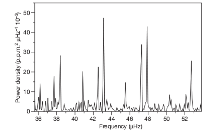
where is the index support of the large entries exceeding in absolute value the threshold . This class contains all vectors for which at most large entries exceed the threshold in absolute value, while the -norm of the other entries stays below a certain noise level. To highlight the concrete modeling potential of such a class, in Figure 1 we show typical examples of real-life signals from Asteroseismology falling into it, for some choice of the parameters .
Let us now informally explain how the class can be crucially used to analyze the effects of noise folding in terms of support recovery depending on the parameters . Therefore, assume now that is a sparse vector with at most nonzero entries exceeding the threshold in absolute value and in expectation (notice that we specified here ). By the statistical equivalence mentioned above of the model (2) and (1), we infer that the recovered vector by means of the Dantzig selector will fulfill the following error estimate:
| (5) |
where the last inequality follows by the requirement
considering here as previously defined in (4). Since we assume that and , the right-hand-side of (1) can be further bounded from above by
It easily follows (and we will use similar arguments below for different decoding methods) that a sufficient condition for the identification of the support of , i.e., , is
or, equivalently,
Notice that such a sufficient condition on actually implies a rather large gap between the significant entries of and the noise components in . Hence, it is of utmost practical interest to understand how small this gap is actually allowed to be, i.e., how large can be relatively to , for the most used recovery algorithms in compressed sensing (not only the Dantzig selector) to be able to have both support identification and a good approximation of the significant entries of .
An approach to control the noise folding, is proposed in [2]. In this case, one may tune the linear measurement process in order to a priori filter the noise. However, this strategy requires to have a precise knowledge of the noise statistics and to design proper filters. Other related work [21, 22, 23] addresses the problem of designing adaptive measurements, called distilled sensing, in order to detect and locate the signal within white noise.
In this paper, we shall follow a blind-to-statistics approach (although, as recalled below, we do not consider the scenario of impulsive noise), which does not modify the non-adaptive measurements, and, differently from the Dantzig selector analysis in [8], we restrict ourself to a purely deterministic setting.
First of all, we show that, unfortunately, the classical -minimization, but also the iteratively re-weighted -minimization [10, 27], considered one of the most robust in the field, easily fails in both the tasks mentioned above as soon as . The deep reason of this failure is the lack of selectivity of these algorithms, which are designed to promote not only the sparsity of the signal but also of the recovered noise. This principle drawback affects necessarily also recent modifications of re-weighted -minimization as appearing in [25].
This has the consequence, as a sort of balancing principle, that the miscomputed components of the noise , if it is not originally of impulsive nature, blow up the inaccuracy in the detection and approximation of . (Notice that the problem of separating sparse signals within impulsive noise is much harder and it will not be considered within the scope of the present paper.)
To overcome these difficulties of these popular methods, we propose a new decoding procedure, combining -minimization and regularized selective least -powers, which is able to reduce the noise component affecting the signal and also to enhance the support identification. In fact, for certain applications, such as radar [24], the support recovery can be even more relevant than an accurate estimate of the signal values. Although the analysis and the numerical results of this new procedure greatly
outperform -minimization and its re-weighted iterative version, its computational complexity becomes prohibitive in very high-dimension. For we conclude by proposing and analyzing an eventual method, based on similar principles, which combines again a warm-up step based on -minimization with a nonconvex optimization realized by the well-known iterative hard thresholding [7], and a final correction step realized by a convex optimization. We show that this latter method performs as robustly as the previous one, but with a drastic reduction of the complexity.
The paper is organized as follows. In the next section, we concisely recall the pertinent features of the theory of compressive sensing. In Section 3, we shall describe the limitations of -minimization when noise on the signal is present, and we mention that very similarly an analogue analysis can be performed for the iteratively re-weighted -minimization based on the results in [27]. Afterwards, as an alternative, we propose the linearly constrained minimization of the regularized selective -potential functional, and show that certain sufficient conditions for recovery indicate significantly better performance than the one provided by -minimization and iteratively re-weighted -minimization. Within this paper, we measure the performance of a method by its ability to identify and approximate the relevant entries of the original signal, where the relevant entries of a signal are the ones which exceed a predefined threshold . For this purpose, we introduced the class (4). With respect to the notation in the introduction, this class is changing the meaning of the notation throughout the rest of the paper and makes redundant the notation , which emphasizes the fact that the noise is directly on the signal. Section 4 recalls the main properties of a very robust and efficient algorithm to perform the linearly constrained minimization of the regularized selective least -powers. In Section 5, we address the issue of the high computational cost of the regularized selective -potential optimization and propose, exploiting a similar selectivity principle, an alternative method based on iterative hard thresholding. Finally, in Section 6, we report the results of extensive numerical experiments, which we made to illustrate and support our theoretical guarantees, and the comparisons between all the mentioned decoding methods.
2 Compressive sensing
It is possible to uniquely and robustly identify the solution of the linear system for an arbitrary given measurement vector , if has rank , and . However, in many applications, we may be either not able to take enough measurements, or interested in taking much fewer measurements to save costs or time, i.e., . The theory of compressive sensing studies this scenario under some restrictions, and assumes that the original signal is nearly sparse. In this section, we recall concisely terms and principles of this theory, and we refer to some of the known tutorials for more details [4, 9, 19, 17].
In compressive sensing, we call the matrix the encoder which transforms the -dimensional signal into to the measurement vector of dimension . Further, we assume to have rank from now on in this article. In practice, we do not know and wonder if it is possible to recover it somehow robustly by an efficient nonlinear decoder . As already mentioned, the theory only works if we assume the signal to be sparse or at least compressible.
Definition 1 (-sparse vector).
Let , . We call the vector -sparse if
where denotes the support of .
In applications, signals are often not exactly sparse but at least compressible. We refer to [26] for more details. We define compressibility in terms of the best -term approximation error with respect to the -norm, given by
Definition 2 (Best -term approximation).
Let be an arbitrary vector in . We denote the best k-term approximation of by
and the respective best -term approximation error of by
Remark 1.
The best -term approximation error is the minimal distance of to a -sparse vector. Informally, vectors having a relatively small best -term approximation error are considered to be compressible.
Remark 2.
If we define the nonincreasing rearrangement of by
then
Alternatively, we can describe the best--term approximation error by
where , and is its complement in .
A desirable property of an encoder/decoder pair is given by the following stability estimate, called instance optimality
| (6) |
for all , with a positive constant independent of , and the closest possible to [12]. This would in particular imply that by means of we are able to recover a -sparse signal exactly, since in this case . It turns out that the existence of such a pair restricts the range of to be maximally of the order of . We refer to [5, 12, 16] for more details.
Actually, the above mentioned condition (6) can be realized in practice, at least for , by pairing the -minimization as the decoder with the choice of an encoder which has the so-called Null Space Property of optimal order . (For realizations of the instance optimality in other -norms, for instance for , one needs more restrictive requirements, see [33]. For the analysis within this paper, we shall use (6) just for for the sake of simplicity.)
Definition 3 (Null Space Property).
A matrix has the Null Space Property of order and for positive constant if
for all and all such that . We abbreviate this property with the writing -NSP.
The Null Space Property states that the kernel of the encoding matrix contains no vectors where some entries have a significantly larger magnitude with respect to the others. In particular, no compressible vector is contained in the kernel. This is a natural requirement since otherwise no decoder would be able to distinguish a sparse vector from zero.
Lemma 1.
Let have the -NSP, with , and define
the set of feasible vectors for the measurement vector . Then the decoder
| (7) |
which we call -minimization, performs
| (8) |
for all and the constant .
Although the result we stated here is by now well-known, see also [31], we report its short proof for the sake of completeness, and for comparison with the enhanced guarantees given in Theorem 4 below.
Proof.
Let us denote and . Then and
because is a solution of the -minimization problem (7). Let be the set of the -largest entries of in absolute value. One has
It follows immediately from the triangle inequality that
Hence, by the -NSP
or, equivalently,
| (9) |
Finally, again by the -NSP
and the proof is completed. ∎
Unfortunately, the NSP is hard to verify in practice. Therefore one can introduce another property which is called the Restricted Isometry Property which implies the NSP. Being a spectral concentration property, the Restricted Isometry Property is particularly suited to be verified with high probability by certain random matrices; we mention some instances of such classes of matrices below.
Definition 4 (Restricted Isometry Property).
A matrix has the Restricted Isometry Property (RIP) of order with constant if
for all . We refer to this property by -RIP.
Lemma 2.
Let and . Assume that has -RIP. Then has -NSP, where
The proof of this latter result can be found, for instance, in [17], and not being of specific relevance for this paper we do not include it here, although it will be important at some points below to connect the RIP to a corresponding NSP.
Encoders which have the RIP with optimal constants, i.e., with in the order of exist, but, so far, as mentioned above, they can be realized exclusively by randomization. By now, classical examples of stochastic encoders are i.i.d. Gaussian matrices [16] or discrete Fourier matrices with randomly chosen rows [11]. Further details and generalizations are provided in [19, 29]. In the rest of the paper we will use as prototypical cases mainly such stochastic encoders.
A recent ansatz to increase the reconstruction accuracy of sparse vectors is iteratively re-weighted -minimization [10, 27]. The idea of this approach is to iteratively solve the weighted -minimization
while updating the weights according to for all , for a suitably chosen stability parameter . We denote this decoder by , and recall the following respective instance optimality result.
Lemma 3 ([27, Theorem 3.2]).
Let have the -RIP, with , and assume the smallest nonzero coordinate of in absolute value larger than the threshold
| (10) |
Then the decoder performs
| (11) |
What we recalled up to this point of the theory of compressive sensing tells us that we are able to recover by (iteratively re-weighted) -minimization compressible vectors within a certain accuracy, given by (8) or (11) respectively. If we re-interpret compressible vectors as sparse vectors which are corrupted by noise, we immediately see that the accuracy of the recovered solution is basically driven by the noise level affecting the vector. Nevertheless, neither inequalities (8) and (11) tell us immediately if the recovered support of the largest entries of the decoded vector in absolute value is the same as the one of the original signal nor are we able to identify the large entries exceeding a given threshold in absolute value. Section 3 addresses these issues in detail and investigates the limitations of -minimization and iteratively re-weighted -minimization.
Furthermore, we propose a new decoder, which is able to outperform -minimization and iteratively re-weighted -minimization in terms of simultaneously identifying the exact position of the significant entries and reducing the noise level on the signal.
3 Support identification
We have seen in Lemma 1 that sparse vectors can be recovered exactly by the –minimization decoder if the matrix has the NSP. Moreover, a sparse signal which is disturbed by noise is recovered within a certain accuracy depending on the best -term approximation error. In this section, we investigate in detail the noise level we can tolerate without loosing the ability of -minimization to recover the support of the undisturbed sparse signal.
For later use, let us denote, for and such that ,
| (12) |
3.1 The -minimization result
The following simple proposition shows how we can recover the support of the original signal if we know the -minimizer. It turns out that the large entries of the original signal in absolute value need to exceed a certain threshold, which depends on the noise level.
Theorem 1.
Let be a noisy signal with relevant entries and the noise level , , i.e., for ,
| (13) |
for a fixed . Consider further an encoder which has the -NSP, with , the respective measurement vector , and the -minimizer
If the -th component of the original signal is such that
| (14) |
then .
Proof.
The noise level substantially influences the ability of support identification. Here, the noisy signal should have (as a sufficient condition) the largest entries in absolute value above
in order to guarantee support identification.
3.2 The result for iteratively re-weighted -minimization
We are able also in the case of the iteratively re-weighted -minimization to show a similar support identification result, which follows similarly from Lemma 3.
Theorem 2.
Let be a noisy signal with relevant entries and the noise level , , i.e., for ,
| (18) |
for a fixed . Consider further an encoder which has the -RIP, with , the respective measurement vector , and the iteratively re-weighted -minimizer . If for all
| (19) |
then .
Proof.
As negative aspects , we notice that, in view of (20) already the conditions of Lemma 3 for the stable convergence of the algorithm do imply support identification. Moreover, we stress that Theorem 2 requires the RIP, which is in general a stronger condition than the NSP. Again, one observes that the noise level influences the ability of support identification. Here, the noisy signal should have the largest entries in absolute value above
in order to guarantee support identification.
In the following, we shall show that for the class , as defined in (4), a smaller threshold is required for support identification, under the sole request of the NSP (and not of the RIP).
3.3 Support identification stability in the class
In this section, we present results in terms of support discrepancy once we consider two elements of the class defined in (4), having the same measurements, i.e., they are both in for .
Theorem 3.
Let have the -NSP, for , , and such that , and . Then
| (21) |
(Here we denote by “” the set symmetric difference, not to be confused with the symbol of a generic decoder.) If additionally
| (22) |
then , i.e., we have unique identification of the large entries in absolute value.
Proof.
As , the difference . By the -NSP, Hölder’s inequality, and the triangle inequality we have
| (23) |
Now we estimate the symmetric difference of the supports of the large entries of and in absolute value as follows: if , then either and or and . This implies that . Thus we have
Together with the inequality (23) and the non-negativity of , we obtain the chain of inequalities
and therefore
| (24) |
For the unique support identification, we want the symmetric difference between the sets and to be empty. Thus the left-hand side of inequality (24) has to be zero. Since , it is sufficient to require that the right-hand side be strictly less than one, and this is equivalent to condition (22). ∎
Remark 3.
One additional implication of this latter theorem is that we can give a bound on the difference of and restricted to the relevant entries. Indeed, in case of unique identification of the relevant entries, i.e., we obtain, by the inequality (23), that
| (25) |
Notice that we replaced by , because now .
Remark 4.
Unfortunately, we are not able to provide the necessity of the gap conditions (14), (19), (22) for successful support recovery, simply because we lack optimal deterministic error bounds in general: one way of producing a lower bound would be to construct a counterexample for each algorithm for which a certain gap condition is violated and recovery of support fails. Since most of the algorithms we shall illustrate below are iterative, it is likely extremely difficult to provide such explicit counterexamples. Therefore, we limit ourselves here to discuss the difference of and and of and . We shall see in the numerical experiments that the sufficient gap conditions (14), (19), (22) nevertheless provide actual indications of performance of the algorithms.
-
•
The gap between the two thresholds is given by
As and is very large for , this positive gap is actually very large, for .
-
•
The gap between the two thresholds is given by
Following for example the arguments in [14], we know that the matrix having the -RIP implies having the -NSP with , which, substituted into the above equation, yields
Since , we have , and therefore the denominator and the right summand in the numerator are positive. The left summand of the numerator is positive and very large as soon as . Thus, even in the limiting scenario where , we still have , which may be considered sufficient for a wide range of applications. If one wants to exceed this threshold a more sophisticated estimate of the above term will reveal even less restrictive bounds on . Thus, in general, since and are small, also the left summand is positive. We conclude that again the gap is very large.
Unfortunately, this discrepancy cannot be amended because the -minimization decoder and the iteratively re-weighted -minimization decoder have not in general the property
Hence, it allows us neither to say that also the (iteratively re-weighted) -minimizer has a bounded noise component
nor to apply Theorem 3 to obtain support stability. We present several examples in Section 6, showing these ineliminable limitations of and .
3.4 The regularized selective -potential functional and its properties
To overcome the shortcomings of methods based exclusively on -minimizations in 1. damping the noise-folding and consequently in 2. having a stable support recovery, in this section, we design a new decoding procedure which allows us to have both these very desirable properties.
Let us first introduce the following functional.
Definition 5 (Regularized selective -potential).
We define the regularized truncated -power function by
| (26) |
where , and is the third degree interpolating polynomial
with
| (27) |
The parameters which appeared in the definition of the interpolating function are defined as: , , , , and . Moreover, we define it for as . We call the functional ,
| (28) |
the regularized selective -potential (SP) functional.
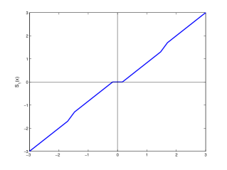
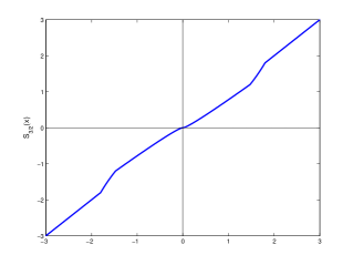
To easily capture the function , we express it explicitly for . In this case, the polynomial has the analytic form
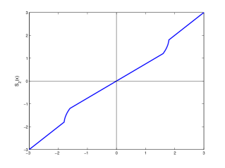
and the graph of is shown in Figure 2 for , , and . Notice that is the truncated p-power function, which is widely used both in statistics and signal processing [3, 18], and also shown in Figure 2 for .

Remark 5.
Let us notice that the functional is semi-convex for , that means that there exists a constant such that is convex.
Theorem 4.
Let have the , with , and . Furthermore, we assume , for , , with the property of having the minimal within , where is its associated measurement vector, i.e.,
| (29) |
If is such that
| (30) |
and
| (31) |
for all , then also , implying noise-folding damping. Moreover, we have the support stability property
| (32) |
Proof.
Notice that we can equally rewrite the functional as
where for . Here, by construction, we have . By the assumptions (30) and , we have
| (33) |
and thus,
As by assumption, the minimality property (29) yields immediately
| (34) |
Assumption (31) and again (30) yield
By this latter inequality and (34) we obtain
which implies . By an application of Theorem 3, we obtain (32). ∎
Remark 6.
Let us comment on the assumptions of the latter result.
-
(i)
The assumption that is actually the vector with minimal essential support among the feasible vectors in corresponds to the request of being the ”simplest” explanation to the data, in a certain sense we acknowledge the Occam’s razor principle;
-
(ii)
The best candidate to fulfill condition (30) would be actually
(35) because this will make (30) true, whichever is. However (35) is a highly nonconvex problem whose solution is in general NP-hard [1]. The way we will circumvent this drawback is to employ an algorithm, which we describe in details in the following section, to compute by âperforming a local minimization of in around a given starting vector . Ideally, the best choice for would be itself, so that (30) may be fulfilled. But, obviously, we do not dispose yet of the original vector . Therefore, a heuristic rule, which we will show to be very robust in our numerical simulations, is to choose , i.e., we use as the result of the -minimization as a warm-up for the iterative algorithm described below. The reasonable hope is that actually
-
(iii)
The assumption that the outcome of the algorithm has additionally the property , for all is justified by observing that in our implementation will be the result of a thresholding operation, i.e., , for , see (38). The particularly steep shape of the thresholding function in the interval , especially for , see Figure 3, makes it highly unlikely for sufficiently small that for . Actually, our numerical experiments confirm that typically this algorithm promotes solutions in selectively characterized by a relevant gap between large components exceeding and small components, significantly below .
4 Minimization of the regularized selective -potential functional
In the latter section, we introduced the functional , which is nonconvex. Unluckily, this makes its linearly constrained minimization (35), which we want to call selective least -powers (SLP), also nontrivial. Here, we recall a novel and very robust algorithm for linearly constrained nonconvex and nonsmooth minimization, introduced and analyzed first in [3]. The algorithm is particularly suited for our purpose, since it only requires a -regular functional. This distinguishes it from other well-known methods such as SQP and Newton methods, which require a more restrictive -regularity. All notions and results written in this section are collected more in general in [3]. Nevertheless we report them directly adapted to our specific case in order to have a simplified and more immediate application.
4.1 The algorithm
In this section, we present the algorithm to perform the local minimization of (28) in . Before describing it, it is necessary to introduce the concept of -convexity, which plays a key-role in the minimization process. In fact, to achieve the minimization of the functional , we use a Bregman-like inner loop, which requires this property to converge with an a priori rate.
Definition 6 (-convexity).
A function is -convex if there exists a constant such that for all and
| (36) |
where is the subdifferential of the function .
The starting values and are taken arbitrarily. For a fixed scaling parameter and an adaptively chosen sequence of integers , we formulate
The reader can notice that the functional , which appears in the algorithm, has not been yet introduced. Indeed, a modification to the functional must be introduced in order to have convexity, which is necessary for the convergence of the algorithm. It is defined as
where is chosen such that the new functional is convex. The finite adaptively chosen number of inner loop iterates is defined by the condition
for a given parameter , which in our numerical experiments will be set to . We refer to [3, Section 2.2] for details on the finiteness of and for the proof of convergence of Algorithm 1 to critical points
of in . According to Remark 6 (ii), and as we will empirically verify in our numerical experiments reported in Section 6, this algorithm finds critical points (hopefully close to a global minimizer) with the desired properties illustrated in Theorem 32,
as soon as we select the starting point by an appropriate warm-up procedure.
Algorithm 1 does not yet specify how to minimize the convex functional
in the inner loop. For that we can use an iterative thresholding algorithm introduced in [3, Section 3.7], inspired by the previous work [18] for the corresponding unconstrained optimization of regularized selective -potentials. This method ensures the convergence to a minimizer and is extremely agile to be implemented, as it is based on matrix-vector multiplications and
very simple componentwise nonlinear thresholdings.
By the iterative thresholding algorithm, we actually equivalently minimize the functional
where we set only for simplicity. The thresholding functions we use are defined in [3, Lemma 3.15] and, for the relevant case , it has the analytic form
| (37) |
where
Note that in case the only part that varies is the one for because the remaining ones do not depend on . We show in Figure 3 the typical shapes of these thresholding functions for different choices of . By means of these thresholding functions, the minimizing algorithm in the inner loop is given by the componentwise fixed point iteration, for ,
| (38) | |||||
We refer to [3, Theorem 3.17] for the convergence properties of this algorithm.
5 Selectivity principle
In Section 3, we showed a certain superiority of the regularized selective least -powers (SLP) in terms of support identification and damping noise-folding. These theoretical results are supported further below in Section 6 by extensive numerical results. However, the realization of the algorithm SLP described above turns out to be computationally demanding as soon as the dimension gets large. Since the computational time is a crucial point when it comes to practical applications, we shall introduce in this section another and more efficient approach based on the same principles to obtain equally good support identification results. The investigations in Section 3 reveal some weakness of the sparsity concept:
The decoders based on -minimization and iteratively re-weighted -minimization prefer sparse solutions and have the undesirable effect of sparsifying also the noise. Thus all the noise may concentrate on fewer entries which, by a balancing principle, may eventually exceed in absolute value the smallest entries of the actual original signal. This makes it impossible to separate the relevant entries of the signal from the noise by only knowing the threshold which bounds the relevant entries from below. On the contrary, SLP follows a selectivity principle, where the recovery process focuses on the extraction of the relevant entries, while uniformly distributing the noise elsewhere. We want now to export this latter mechanism to formulate the method described below.
In the following, we will show that the very well known iterative hard thresholding [7] shows similar support identification properties as SLP while being very efficient in terms of computational time. This method iteratively computes
| (39) |
where
for . It is converging to a fixed point fulfilling
| (40) |
which is a local minimizer of the functional
see [7, Theorem 3] for details. One immediately observes that iterative hard thresholding has a very selective nature: The computed fixed point is a vector with an unknown number, although expected to be small, of non-zero entries whose absolute value is above the threshold . In the following, we show under which conditions this method is able to exactly identify the support of the relevant entries of the original vector .
Theorem 5.
Assume to have the -RIP, with , , and define such that
where are the columns of the matrix . Let , for a fixed , and the respective measurements. Assume further
| (41) |
and define such that
| (42) |
Let be the limit of the iterative hard thresholding algorithm (39), and thus fulfilling the fixed point equation (40). Further, we assume
| (43) |
then we have that , and
| (44) |
Proof.
Assume . By (43), we have that
where the last inequality follows by (42). Since , the upper inequality yields to a contradiction.
Thus and therefore and are both -sparse, and is -sparse. Under our assumptions we can apply [7, Lemma 4] to obtain
| (45) |
In addition to this latter estimate, we use the RIP, the sparsity of , and (42) to obtain for all that
Assume now that there is such that and . But then we would also have , which leads to a contradiction. Thus, we have equivalently . In addition to , this concludes the proof. ∎
Remark 7.
Let us discuss some of the assumptions and implications of this latter result.
-
(i)
Since iterative hard thresholding is only computing a local minimizer of , condition (43) may not be always fulfilled for any given initial iteration . Similarly to the argument in Remark 6 (ii), using the -minimizer as the starting point , or equivalently choosing the vector as composed of the entries of exceeding in absolute value, we may allow us to approach a local minimizer which fulfills (43).
- (ii)
Although we are able to exactly identify the support by means of Theorem 5, we only have the very poor error estimate (44) of the relevant part of the signal. The reason why we cannot obtain an estimate as good as the one in Remark 3 is that the conditions , and to apply Theorem 3 are in general not fulfilled. Hence an additional correction to is necessary. As we now dispose of the support , a natural approach is to seek for an additional vector which is the solution of
| s.t. | (46) | |||
Since the original signal fulfills , and , it is actually a solution of problem (46). Thus, we conclude that for any minimizer of problem (46) the objective function equals zero, thus , and we conclude and as well. The optimization (46) is in general nonconvex, but, luckily, we can easily recast it in an equivalent convex one: Since , and , we know that the relevant entries of and have the same sign. Since we are searching for solutions which are close to , the second inequality constraint becomes , for all . Together with the equivalence of - and -norm, we rewrite problem (46) as
| s.t. | (47) | |||
where is defined componentwise by
and , . Since , , and , , are semi-definite, problem (47) is a convex quadratically constrained quadratic program (QCQP) which can be efficiently solved by standard methods, e.g., interior point methods [28]. Since we combine here three very efficient methods (-minimization, iterative hard thresholding, and a QCQP), the resulting procedure is much faster than the computation of SLP while, as we will show in the numerics, keeping similar support identification properties.
6 Numerical results
The following numerical simulations provide empirical confirmation of the theoretical observations in Section 3 and Section 5. In particular, we want to show that SLP and IHT, initialized by the -minimizer as a starting value, are very robust and provide a significantly enhanced rate of recovery of the support of the unknown sparse vector as well as a better accuracy in approximating its large entries, whenever limiting noise, i.e., , is present on the signal.
In the previous sections we provided a very detailed description of the parameter choice for the concrete implementation of SLP and IHT, which depends in a rather explicit way on the threshold parameter and it is independent of the dimensionalities of the problem. Instead, it turns out to be extremely hard to tune the parameter , appearing in [10, 27] as the -norm residual discrepancy, in order to obtain the best performances for the iteratively re-weighted -minimization (IRW) in terms of support identification and accuracy in approximating the large entries of the original vector. In the papers [10, 27] the authors indicated , depending on , as the best parameter choice for ameliorating the discrepancy in -norm between original and decoded vector with respect to the sole -minimization. However, in our experiments we found out that for the two purposes mentioned above a much smaller has to be chosen. The stability parameter , which avoids the denominator to be zero in the weight updating rule seems to have instead no strong influence, and it is set to 0.1 in our experiments. We executed 8 iterations of IRW as a reasonable compromise between computational effort and accuracy.
We also consider as one of the test methods -minimization, where we substituted the equality constraint with an inequality constraint which takes into account the noise level, folded from the noise on the signal though; thus
In this constraint, we used the same parameter as for IRW.
As we shall argue in detail below, the following numerical tests indicate that +IHT is much faster and usually more robust than +SLP, and that both of them perform much better than -minimization and IRW in terms of support recovery and accuracy in approximating the large entries in absolute value of the original signal.
Advantages of SLP with respect to -minimization
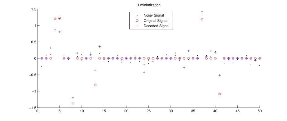
We shall start the discussion on numerical experiments with a comparison between the -minimization and SLP for one typical example reported in Figure 4. Although the setting of the two methods is the same, the results are very different: SLP-minimization can recover the signal with a very good approximation of its large entries in absolute value and a significant reduction of the noise level, while -minimization may approximate the signal in a bad way, due to the amplification of the noise. For instance, it is evident in Subfigure 4 that gives a wrong information about the location of the relevant entries, mismatching them with the noise. However, in this particular example, we were lucky to choose the right starting value for SLP. Due to its nonconvex character, in general SLP is computing a local minimizer, which might be far away from the original signal.
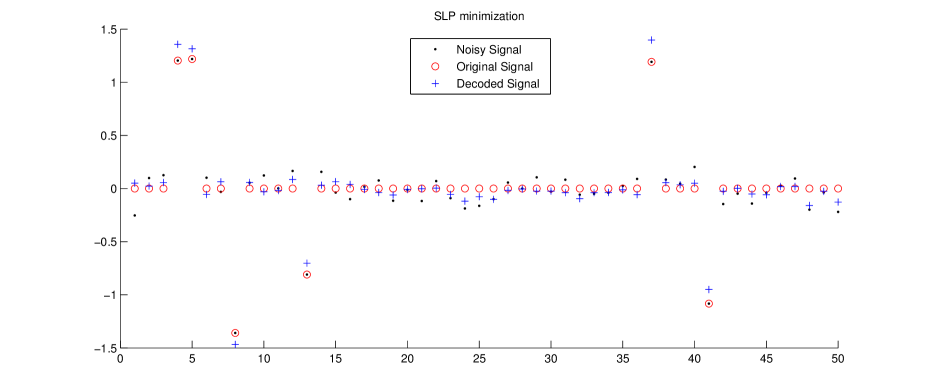
Choosing -minimization as a warm up
In Section 4, we mentioned that the algorithm, which minimizes the functional , finds only a critical point, so the condition (30) used in the proof of Theorem 32 may not be always valid. In order to enhance the chance of validity of this condition, the choice of an appropriate starting point is crucial. As we know that the -minimization converges to its global minimizer with at least some guarantees given by Theorem 1, we use the result of this minimization process as a warm up to select the starting point of Algorithm 1. In the following, we distinguish between SLP which starts at and +SLP which starts at the -minimizer.
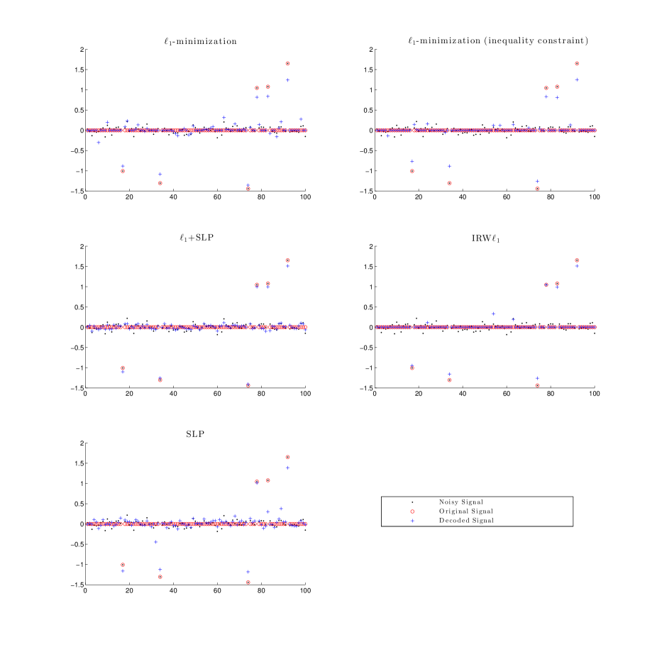
In Figure 5, we illustrate the robustness of +SLP (bottom left subfigure) in comparison to the -minimization based methods and SLP starting at . Here, SLP converged to a feasible critical point, but it is quite evident that the decoding process failed since the large entry at position 83 (signal) was badly recovered and even the entry at position 89 (noise) is larger. If we look at the -minimization result (top left subfigure) or the -minimization with inequality constraint (top right subfigure), the minimization process brings us close to the solution, but the results still significantly lack accuracy. By +SLP (center left subfigure) we obtain a good approximation of the relevant entries of the original signal and we get a significant correction and an improved recovery. Also IRW improves the result of -minimization significantly, but still approximates the large entries worse than +SLP. Although the difference is minor, we observe another important aspect of IRW: the noise part is sparsely recovered, while +SLP distributes the noise in a more uniform way in a much smaller stripe around zero. This drawback of IRW can be crucial when it comes to the distinction of the relevant entries from noise.
Massive computations
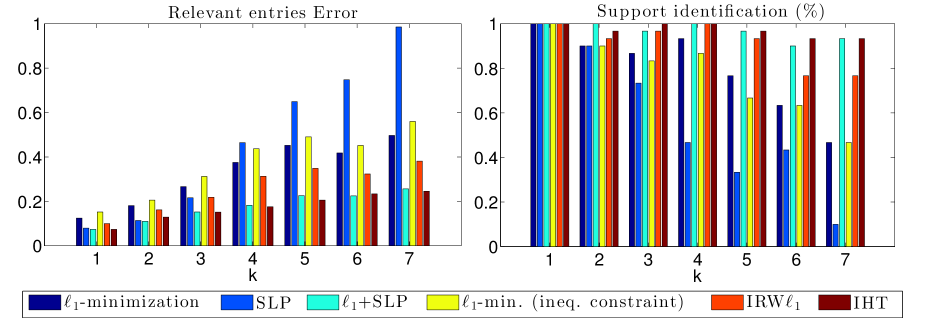
The previously presented specific examples in support of our new decoding strategies are actually typical. In order to support this work with even more impressive and convincing evidences, we present some statistical data obtained by solving series of problems. We decided to fix the parameters in order to have the most coherent data to be analyzed; in particular, we set , , , , and . The vector is composed of random entries with normal distribution and then it is rescaled in order to have . Figures 6, 7, and 8 report the results obtained considering 30 different i.i.d.Gaussian encoding matrices while Figures 9, 10, and 11 used 30 random subsampled cosine transformation encoding matrices. In the following, we use generically for the decoded vector of any method.
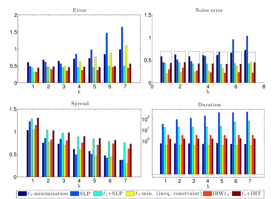
Figure 6 reports the first part of the statistics which we have collected for the Gaussian matrices. We start commenting the subfigures clockwise. The first subfigure, on the upper-left, represents the mean value of the error between the exact signal and the decoded one . For +SLP, +IHT, and IRW the absolute -norm discrepancy between original and decoded vector seems to be stable and independent of the number of large entries. These methods outperform -minimization; IRW performs slightly better. We also observe that the choice of the starting point is crucial for SLP and IHT.
The second subfigure is the mean value of the noise level and we can see exactly what we inferred looking at Figure 5: -minimization returns a larger noise level with respect to all the other methods, except SLP; and IRW has the best noise reduction property.
The third is the mean computational time, presented in logarithmic scale. All tests were implemented and run in Matlab R2013b in combination with CVX [13, 20], to solve the -minimization with equality and inequality constraint, its iteratively re-weighted version, and the QCQP. We observe that SLP and +SLP are extremely slow. However, in comparison, the good starting point for SLP provides an advantage in terms of computational time. IHT has a computational complexity in between -minimization and IRW.
The fourth plot reports the mean value of the discrepancy between noise level and the large entries of the signal, thus
. This plot shows how good the small entries are distinguished from the large ones in absolute value. We see that +SLP and +IHT perform best, which again is a result of their non-sparse noise recovery.
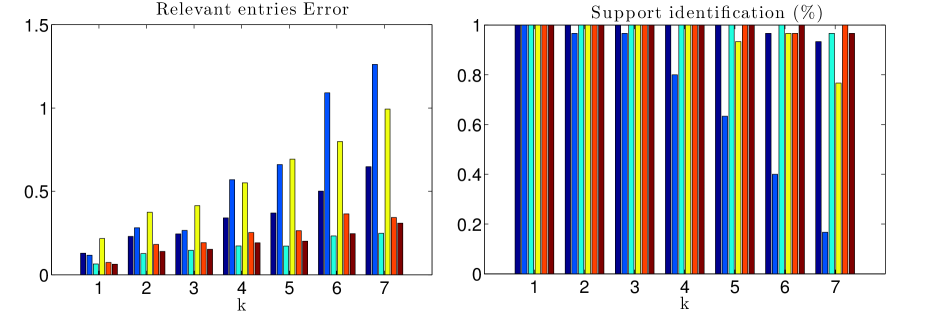
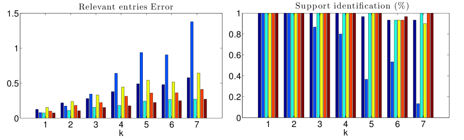
In Figure 7, we report the histogram of the mean-value of the errors on the relevant entries: the quantities on the left subfigure are computed as the mean values of where we suppose to know the largest entries of the original signal. The right subfigure shows how often the largest entries of coincided with . Notice that there might be entries below the threshold among the largest entries of . We conclude that, knowing the number of large entries, IRW, -minimization, +SLP, and +IHT recover the support with nearly 100% success. In addition, +SLP approximates best the magnitudes of the relevant entries.
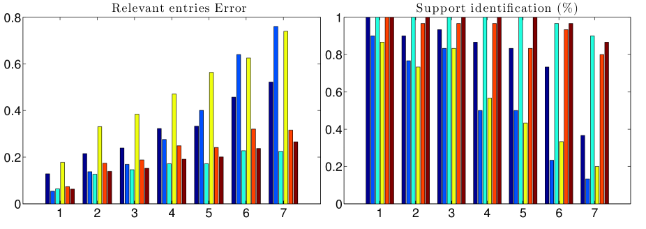
In Figure 8 we compute again the mean-value of the relevant entries, but this time without the knowledge of but the knowledge of and therefore : the quantities on the left subfigure are the mean values of . In the right subfigure we attribute a positive match in case so that the relevant entries of coincide with the ones of the original signal. By our theory, we expect +SLP and +IHT to produce a high rate of success of correctly recovered support. Actually this is confirmed by the experiments: Both methods do a very accurate recovery, as it gives us almost always of the correct result while the other methods perform worse.
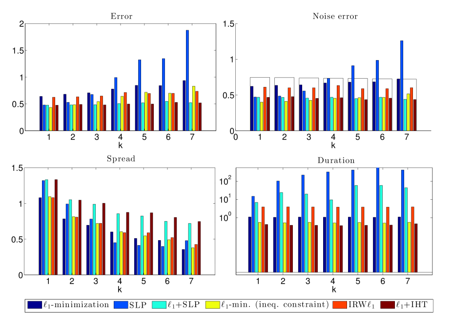
Figures 9, 10, and 11 represent the same statistical data reported respectively in the Figures 6, 7, and 8 but using random subsampled cosine transformation encoding matrices. Without describing the result in detail, we state that they are very similar for these problems as well.
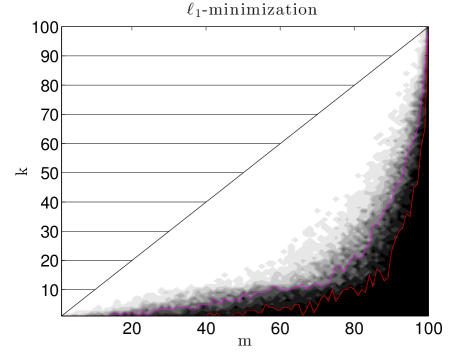
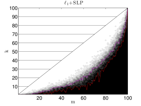
Phase transition diagrams
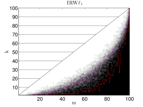
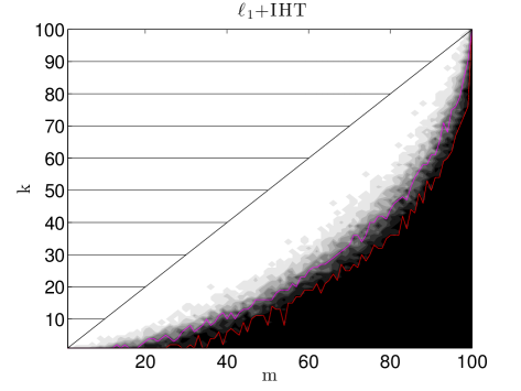
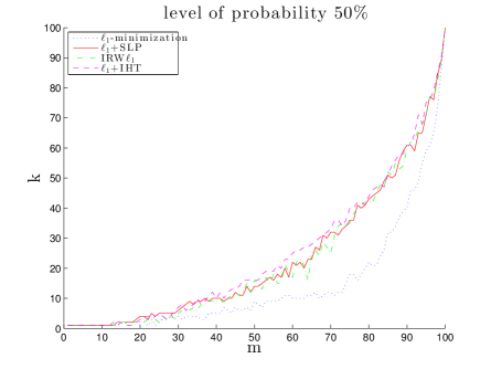
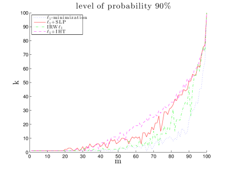
To give an even stronger support of the results in the previous paragraph, we extended the results of Figure 8 to a wider range of and . In Figure 12, we present phase transition diagrams of success rates in support recovery for -minimization, IRW, SLP, and +IHT in presence of nearly maximally allowed noise, i.e., .
To produce phase transition diagrams, we varied the dimension of the measurement vector with , and solved 20 different problems for all the admissible . We colored black all the points , with , which reported 100% of correct support identification, and gradually we reduce the tone up to white for the 0% result. The level bound of 50% and 90% is highlighted by a magenta and red line respectively. A visual comparison of the corresponding phase transitions confirms our previous expectations. In particular, +SLP and +IHT very significantly outperform -minimization in terms of correct support recovery. The difference of both methods towards IRW is less significant but still important. In Figure 13, we compare the level bounds of 50% and 90% among the four different methods. Observe that the 90% probability bound indicates the largest positive region for +IHT, followed by +SLP, and only eventually by IRW, while the bounds are much closer to each other in the case of the 50% bound. Thus, surprisingly, +IHT works in practice even better than +SLP for some range of , and offers the most stable support recovery results.
Funding
Marco Artina acknowledges the support of the International Research Training Group IGDK 1754 “Optimization and Numerical Analysis for Partial Differential Equations with Nonsmooth Structures” of the German Science Foundation. Massimo Fornasier acknowledges the support of the ERC-Starting Grant HDSPCONTR “High-Dimensional Sparse Optimal Control”. Steffen Peter acknowledges the support of the Project “SparsEO: Exploiting the Sparsity in Remote Sensing for Earth Observation” funded by Munich Aerospace.
References
- [1] B. Alexeev and R. Ward. On the complexity of Mumford-Shah-type regularization, viewed as a relaxed sparsity constraint. IEEE Trans. Image Process., 19(10):2787–2789, 2010.
- [2] E. Arias-Castro and Y. C. Eldar. Noise folding in compressed sensing. IEEE Signal Process. Lett., pages 478–481, 2011.
- [3] M. Artina, M. Fornasier, and F. Solombrino. Linearly constrained nonsmooth and nonconvex minimization. SIAM J. Opt., 23,(3):1904–1937, 2012.
- [4] R. Baraniuk. Compressive sensing. IEEE Signal Process. Magazine, 24(4):118–121, 2007.
- [5] R. G. Baraniuk, M. Davenport, R. A. DeVore, and M. Wakin. A simple proof of the restricted isometry property for random matrices. Constr. Approx., 28(3):253–263, 2008.
- [6] T. R. Bedding and H. Kjeldsen. Solar-like oscillations. Publications of the Astronomical Society of Australia, 20(2):203–212, 2003.
- [7] T. Blumensath and M. E. Davies. Iterative thresholding for sparse approximations. Journal of Fourier Analysis and Applications, 14(5-6):629–654, 2008.
- [8] E. Candes and T. Tao. The Dantzig selector: Statistical estimation when p is much larger than n. The Annals of Statistics, 35(6):2313–2351, 2007.
- [9] E. Candès and M. Wakin. An introduction to compressive sampling. IEEE Signal Process. Magazine, 25(2):21–30, 2008.
- [10] E. Candès, M. Wakin, and S. Boyd. Enhancing sparsity by reweighted minimization. Journal of Fourier Analysis and Applications, 14(5-6):877–905, 2008.
- [11] E. J. Candès, J. Romberg, and T. Tao. Stable signal recovery from incomplete and inaccurate measurements. Comm. Pure Appl. Math., 59(8):1207–1223, 2006.
- [12] A. Cohen, W. Dahmen, and R. A. DeVore. Compressed sensing and best -term approximation. J. Amer. Math. Soc., 22(1):211–231, 2009.
- [13] I. CVX Research. CVX: Matlab software for disciplined convex programming, version 2.0. http://cvxr.com/cvx, 2012.
- [14] M. Davenport. The RIP and the NSP. @Connexions. http://cnx.org/content/m37176/1.5/, Apr. 2011.
- [15] M. A. Davenport, J. N. Laska, J. R. Treichler, and R. G. Baraniuk. The pros and cons of compressive sensing for wideband signal acquisition: Noise folding vs. dynamic range. IEEE Transactions on Signal Processing, 60(9):4628–4642, 2012.
- [16] D. L. Donoho. Compressed sensing. IEEE Transactions on Information Theory, 52(4):1289–1306, 2006.
- [17] M. Fornasier and H. Rauhut. Compressive Sensing. In O. Scherzer, editor, Handbook of Mathematical Methods in Imaging, pages 187–228. Springer, 2011.
- [18] M. Fornasier and R. Ward. Iterative thresholding meets free-discontinuity problems. Found. Comput. Math., 10(5):527–567, 2010.
- [19] S. Foucart and H. Rauhut. A Mathematical Introduction to Compressive Sensing. Appl. Numer. Harmon. Anal. Birkhäuser, Boston, 2013.
- [20] M. Grant and S. Boyd. Graph implementations for nonsmooth convex programs. In V. Blondel, S. Boyd, and H. Kimura, editors, Recent Advances in Learning and Control, Lecture Notes in Control and Information Sciences, pages 95–110. Springer-Verlag Limited, 2008. http://stanford.edu/boyd/graphdcp.html.
- [21] J. Haupt, R. Baraniuk, R. Castro, and R. Nowak. Compressive distilled sensing: Sparse recovery using adaptivity in compressive measurements. In Proceedings of the 43rd Asilomar conference on Signals, systems and computers, Asilomar’09, Piscataway, NJ, USA, 2009. IEEE Press.
- [22] J. Haupt, R. Baraniuk, R. Castro, and R. Nowak. Sequentially designed compressed sensing. In Proc. IEEE/SP Workshop on Statistical Signal Processing, 2012.
- [23] J. Haupt, R. Castro, and R. Nowak. Distilled sensing: Adaptive sampling for sparse detection and estimation. IEEE Transactions on Information Theory, 57(9):6222–6235, 2011.
- [24] M. Hügel, H. Rauhut, and T. Strohmer. Remote sensing via -minimization. Preprint, 2012.
- [25] M. A. Khajehnejad, W. Xu, A. S. Avestimehr, and B. Hassibi. Improved sparse recovery thresholds with two-step reweighted minimization. In ISIT, pages 1603–1607, 2010.
- [26] S. Mallat. A Wavelet Tour of Signal Processing: The Sparse Way. Academic Press, 3rd edition, 2008.
- [27] D. Needell. Noisy signal recovery via iterative reweighted l1-minimization. In Proceedings of the 43rd Asilomar conference on Signals, systems and computers, Asilomar’09, pages 113–117, Piscataway, NJ, USA, 2009. IEEE Press.
- [28] J. Nocedal and S. J. Wright. Numerical optimization. Springer Series in Operations Research and Financial Engineering. Springer, New York, second edition, 2006.
- [29] H. Rauhut. Compressive sensing and structured random matrices. In M. Fornasier, editor, Theoretical Foundations and Numerical Methods for Sparse Recovery, volume 9 of Radon Series Comp. Appl. Math., pages 1–92. deGruyter, 2010.
- [30] J. D. Ridder, C. Barban, F. Baudin, F. Carrier, A. P. Hatzes, S. Hekker, T. Kallinger, W. W. Weiss, A. Baglin, and M. Auvergne. Non-radial oscillation modes with long lifetimes in giant stars, 2009.
- [31] M. Stojnic, W. Xu, A. S. Avestimehr, and B. Hassibi. Compressed sensing of approximately sparse signals. In ISIT, pages 2182–2186, 2008.
- [32] J. Treichler, M. A. Davenport, and R. G. Baraniuk. Application of compressive sensing to the design of wideband signal acquisition receivers. In 6th U.S. / Australia Joint Workshop on Defense Applications of Signal Processing (DASP), Lihue, Hawaii, Sept. 2009.
- [33] P. Wojtaszczyk. Stability and instance optimality for Gaussian measurements in compressed sensing. Found. Comput. Math., 10(1):1–13, 2010.
- [34] D. Wu, W.-P. Zhu, and M. Swamy. Compressive sensing based speech enhancement in nonsparse noisy environments. IET Signal Processing, 7(5):450–457, 2013.
- [35] D. Wu, W.-P. Zhu, and M. Swamy. A note on error bounds of compressed sensing in considering nonsparse noise from the time domain. preprint, 2014.