Synchronisation and liquid crystalline order in soft active fluids.

Abstract

We introduce a phenomenological theory for a new class of soft active fluids, with the ability to synchronise. Our theoretical framework describes the macroscopic behaviour of a collection of interacting anisotropic elements with cyclic internal dynamics and a periodic phase variable. This system (i) can spontaneously undergo a transition to a state with macroscopic orientational order, with the elements aligned: a liquid crystal, (ii) attain another broken symmetry state characterised by synchronisation of their phase variables or (iii) a combination of both types of order. We derive the equations describing a spatially homogeneous system and also study the hydrodynamic fluctuations of the soft modes in some of the ordered states. We find that synchronisation can promote the transition to a state with orientational order; and vice-versa. Finally, we provide an explicit microscopic realisation : a suspension of micro-swimmers driven by cyclic strokes.

Active materials are composed of self-driven units, active particles, each capable of converting stored or ambient free energy into systematic movement and performing work on their surrounding environment Marchetti et al. (2013). The interaction of active particles with each other, and with the medium they live in, gives rise to highly correlated collective motion. Examples include micro-swimmers suspended in a fluid Lauga and Powers (2009), motor protein-filaments mixtures, such as those forming the cell cytoskeleton Toner and Tu (1995); Aditi Simha and Ramaswamy (2002); Kruse et al. (2005); Ahmadi et al. (2006) and cells forming tissues Sachs (1991). They have non-conventional properties, such as anomalous viscosities Sokolov and Aranson (2009); Rafai et al. (2010), and the ability to self-organise into ordered states Sokolov et al. (2007), with local alignment, forming patterns Riedel et al. (2005) and favouring collective transport on scales larger than individual Dombrowski et al. (2004). There is wide and growing body of theoretical work focussed on investigating the collective dynamics, picturing the individuals as static force-multipoles Aditi Simha and Ramaswamy (2002); Kruse et al. (2005); Saintillan and Shelley (2008); Baskaran and Marchetti (2009) interacting in a fluid or by generic rules of alignment Ginelli et al. (2010). However at the microscopic level, the dynamics of active individuals is often time-dependent and cyclic - breaking time-translational invariance. The effect of this on their collective behaviour is much less well understood. Recently, this has been studied for swimmers with identical cycles by coarse-graining simple dynamical microscopic models Leoni and Liverpool (2010a). Whilst this has provided insight, linking the static force multipoles to time averages over the internal cycles, it is missing an important property of the system. In reality the cycles of the individual elements are only identical to within an arbitrary phase revealing another symmetry. Therefore the active constituents typically have the ability to vary their dynamic cycles and synchronise their phases via hydrodynamic (or other) interactions thus breaking this phase symmetry. The effect on the macroscopic behaviour of active fluids of this possible broken symmetry is the subject of this letter. We note that the subject of hydrodynamic synchronisation of micron-sized oscillators is a major topic in its own right with a long history going back to studies of the coordination of pairs of beating flagella or arrays of cilia beating in a fluid Taylor (1951); Guirao and Joanny (2007). There have been an increasing number of recent experimental studies of systems investigating the phenomenon in-vivo Polin et al. (2009); Goldstein et al. (2009), in vitro Sanchez et al. (2011) and in minimal artificial systems Kotar et al. (2010); Qian et al. (2009). This has been paralleled by a recent upsurge in theoretical interest  Kim and Powers (2004); Reichert and Stark (2005); Vilfan and Julicher (2006); Guirao and Joanny (2007); Niedermayer et al. (2008); Uchida and Golestanian (2010); Leoni and Liverpool (2012),

In this letter we address the interplay of phase-synchronisation and orientational dynamics in soft active fluids considering a minimal model which consists of active elements with both an orientation and an internal cycle. The cycle is characterised by a phase variable which varies slowly with time. We define synchronisation with reference to the phase dynamics and say it has occurred when the phases of different individuals are locked at a fixed phase difference. Here we shall consider only in-phase synchronisation, with the phases fixed at the same value, i.e. the phase difference is zero. Synchronisation thus viewed is then simply a type of long range order. Hence, in addition to the usual slow (Nambu-Goldstone) modes describing liquid crystalline fluids and gels de Gennes and Prost (1995); Kruse et al. (2005); Ahmadi et al. (2006), which are associated with broken rotational symmetry, a theory taking account of synchronisation of the active elements requires another slow mode which is associated with the broken symmetry of the phase and has no classical equilibrium analogue.

We identify the order parameters of the system (from the possible broken internal symmetries - $U(1)\times SO(d)$ in $d$-dimensions) and the conserved quantities, then obtain the phenomenological equations for their dynamics by including all the terms allowed by symmetry. We discuss the interplay of synchronisation and orientational dynamics and find that each type of order may promote the occurrence of the other. This is supported by a particular microscopic realisation of the system : a suspension of model swimmers driven by internal cycles with varying phase interacting via hydrodynamic interactions.

Systems where phase and orientation dynamics are uncoupled

To start, we consider a system with both orientational and phase dynamics but where the two are decoupled. For concreteness, we focus on polar fluids Kruse et al. (2005); Ahmadi et al. (2006), characterised by a mean orientational axis $\mathbf{P}$ describing states that are not invariant under transformations $\mathbf{P}\to-\mathbf{P}$. A nematic system, whose mean orientational axis $\hat{\bm{n}}$ is invariant under transformations $\hat{\bm{n}}\to-\hat{\bm{n}}$, can be dealt with using similar techniques Leoni and Liverpool (2013). We consider a large number $N$ of microscopic elements, at positions ${\bf r}_{k}(t)$, $k=1,\ldots N$ in a volume $\mathcal{V}$. Each one is characterised by both fluctuating orientations $\hat{\bm{u}}_{k}(t)$ and phases $\phi_{k}(t)\in(0,2\pi)$. The source of fluctuations is in general a combination of thermal and non-thermal effects.

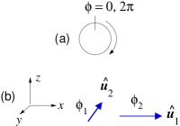
Figure 1: (a) The phase variable $\phi$ associated with the internal cycle. Two elements with orientations $\hat{\bm{u}}_{1}$ and $\hat{\bm{u}}_{2}$ and phases $\phi_{1},\phi_{2}$. To visualise the phase we schematically represent it as the length of the arrow.

A local measure of orientational order is the polar vector, $\mathbf{P}({\bf r},t):=\langle\frac{1}{N}\sum^{N}_{k=1}\hat{\bm{u}}_{k}(t)\delta({\bf r}-{\bf r}_{k})\rangle$ where $\langle\rangle$ represents an average over the fluctuations. Similarly a local measure of synchronisation is the complex-valued quantity Acebrón et al. (2005); Leoni and Liverpool (2012) $\Phi({\bf r},t):=\langle\frac{1}{N}\sum^{N}_{k=1}e^{i\phi_{k}(t)}\delta({\bf r}-{\bf r}_{k})\rangle$. In this letter, we only consider situations where the density, $\rho:=N/\mathcal{V}$ is constant.

The average (bulk) dynamics of the polar active system is captured by $\mathbf{P}_{0}(t)=\int_{r}\mathbf{P}({\bf r},t)$ with an equation of motion Kruse et al. (2005); Ahmadi et al. (2006); Leoni and Liverpool (2010a), $\partial_{t}\mathbf{P}_{0}=b\mathbf{P}_{0}-b^{{}^{\prime}}\|\mathbf{P}_{0}\|^{2}\mathbf{P}_{0}$. The coefficients $b,b^{{}^{\prime}}$ are real valued quantities. $b$ may depend on the density. For swimmers it may also depend on the sign of the average force-dipole Leoni and Liverpool (2010a) of the individuals, while $b^{{}^{\prime}}>0$ stabilises the magnitude, $P:=\|\mathbf{P}_{0}\|$ which measures the amount of orientational alignment of the elements, i.e. polar order. The transition to order is determined by the sign of the coefficient $b$ Ahmadi et al. (2006); Leoni and Liverpool (2010a): the value $b=0$ defines the boundary between the orientational disordered phase, where $b<0$ and the fixed point $P=0$ is stable; and polar phase, where $b>0$ the fixed point $P=0$ becomes unstable. A generic equation describing bulk synchronisation, $\mathbf{\Phi}_{0}(t)=\int_{r}\mathbf{\Phi}({\bf r},t)$ previously considered by us Leoni and Liverpool (2012), is $\partial_{t}\Phi_{0}=a\Phi_{0}-a^{{}^{\prime}}|\Phi_{0}|^{2}\Phi_{0}$. The coefficients $a,a^{{}^{\prime}}$, are complex valued quantities Leoni and Liverpool (2012). For the following analysis it suffices to focus on their real part $\zeta:=Re[a]$ and $\zeta^{\prime}:=Re[a^{{}^{\prime}}]$. $\zeta$ can depend on the density as well as on the isochrony  of the oscillations Leoni and Liverpool (2012). $\zeta^{\prime}>0$ is a stabilising term. Writing $\Phi_{0}=Me^{iQ}$, the magnitude $M$ is a measure of amount of synchronisation of the elements and quantifies this type of order. When $\zeta<0$ the fixed point $M=0$ is stable and the synchronisation occurs when $\zeta>0$ and $M\neq 0$. Hence $\zeta=0$ is the boundary between non-synchronised and synchronised states. The result of this uncoupled dynamics can be conveniently summarised as a phase diagram in the plane $(\zeta,b)$, where each phase (disordered, polar, synchronised $\&$ polar, synchronised) occupies exactly one quadrant, starting from $(\zeta<0,b<0)$ in clockwise order. The interplay of orientational dynamics and synchronisation can shift some of the boundaries of such a phase diagram, as we will discuss below.

Systems where phase and orientation dynamics are coupled

We consider now the average dynamics for this more general case. This system is characterised by the density, $\rho$, the polar vector, $\mathbf{P}_{0}(t)$, and the global phase $\Phi_{0}(t)$ defined above. In addition, we must introduce the complex-valued phase-orientation vector $\bm{\Pi}({\bf r},t):=\langle\frac{1}{N}\sum^{N}_{k=1}e^{i\phi_{k}(t)}\hat{\bm{u}}_{k}(t)\delta({\bf r}-{\bf r}_{k})\rangle$ which encodes the phase-orientation coupling. As before we can define a bulk value, $\bm{\Pi}_{0}(t)=\int_{r}\bm{\Pi}({\bf r},t)$. We can understand its physical significance as follows. When (i) all the orientations are identical, $\hat{\bm{u}}_{k}(t)\equiv\hat{\bm{u}}(t)$ or $(ii)$ when all the phases are locked, $e^{i\phi_{k}(t)}=e^{i\phi(t)}$ $\forall\;k$, $\bm{\Pi}_{0}(t)\equiv\Phi_{0}(t)\mathbf{P}_{0}(t)$. However, when there is partial order of both of the fields, $\bm{\Pi}_{0}(t)\neq\Phi_{0}(t)\mathbf{P}_{0}(t)$. A simple example showing that $\bm{\Pi}_{0}$ may be non-zero, despite having $\mathbf{P}_{0}=0$ and $\Phi_{0}=0$ is a system of 2 particles with values $\hat{\bm{u}}_{1}(t)=-\hat{\bm{u}}_{2}=\hat{\bm{u}}(t)$ and $e^{i\phi_{1}(t)}=-e^{i\phi_{2}(t)}=e^{i\phi(t)}$. The variables $\mathbf{P}_{0}(t)$, $\Phi_{0}(t)$ and $\bm{\Pi}_{0}(t)$ are dynamically coupled. Equations of motion can be obtained by including all the possible terms allowed by the symmetries. For simplicity we shall restrict ourselves to the leading order coupling terms, which are quadratic functions.

In presence of coupling to orientational dynamics, the equation for $\Phi_{0}$ becomes

$$\partial_{t}\Phi_{0}=a\Phi_{0}-a^{{}^{\prime}}|\Phi_{0}|^{2}\Phi_{0}+g\mathbf{P}_{0}\cdot\bm{\Pi}_{0}+\ldots$$ (1)

Here $g$ is a complex-valued coefficient. As eq (1) describes a scalar quantity, all its terms can be understood using configurations where the particles are aligned. Since it is quadratic, the last term can be understood using 2 particles. A finite $\mathbf{P}_{0}$ means that the configurations (a) $\hat{\bm{u}}_{1}(t)=\hat{\bm{u}}_{2}(t)=\hat{\bm{u}}(t)$, of fig 2(a), and (b) $\hat{\bm{u}}_{1}(t)=-\hat{\bm{u}}_{2}(t)=\hat{\bm{u}}(t)$, of fig 2(b), both of which have phases $\phi_{1}(t)$, $\phi_{2}(t)$, should contribute differently to the equation. Using the definitions above, in case (a) one finds $\mathbf{P}_{0}\cdot\bm{\Pi}_{0}=P_{0}^{2}\Phi_{0}$; whereas in case (b), $\mathbf{P}_{0}\cdot\bm{\Pi}_{0}=0$.

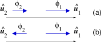
Figure 2: Elements that are aligned but have different phases. (a) and (b) contribute differently to $\bm{\Pi}_{0}\cdot\mathbf{P}_{0}$.

The dynamics of the polar vector becomes

$$\partial_{t}\mathbf{P}_{0}=b\mathbf{P}_{0}-b^{{}^{\prime}}\|\mathbf{P}_{0}\|^{2}\mathbf{P}_{0}+h\Phi_{0}^{*}\bm{\Pi}_{0}+h^{*}\Phi_{0}\bm{\Pi}_{0}^{*}+\ldots$$ (2)

where $h$ is a complex-valued coefficient. Finally, we introduce the equation for the complex polar vector $\bm{\Pi}_{0}$

$$\partial_{t}\bm{\Pi}_{0}=q\bm{\Pi}_{0}-q^{{}^{\prime}}\|\bm{\Pi}_{0}\|^{2}\bm{\Pi}_{0}+m\Phi_{0}\mathbf{P}_{0}+\ldots$$ (3)

Here the coefficients $q,q^{{}^{\prime}},m$ are complex-valued quantities. $q$ may depend on the density and we consider $Re[q^{{}^{\prime}}]>0$ providing a stabilising term. We can get a simple explanation of the last term in eq (2), coupling $\Phi_{0}$, $\bm{\Pi}_{0}$, and the last term in eq (3), coupling $\mathbf{P}_{0}$, $\Phi_{0}$, by considering 2 particles, with orientations $\hat{\bm{u}}_{1}(t),\hat{\bm{u}}_{2}(t)$ and phases $\phi_{1}(t),\phi_{2}(t)$. Then using the definition of $\mathbf{P}_{0}$ and $\bm{\Pi}_{0}$ and taking the time derivatives, $\partial_{t}\mathbf{P}_{0}=\frac{1}{2}[\dot{\hat{\bm{u}}}_{1}+\dot{\hat{\bm{u}}}_{2}]$ and $\partial_{t}\bm{\Pi}_{0}=\frac{1}{2}\sum^{N}_{k=1}e^{i\phi_{k}}[\dot{\hat{\bm{u}}}_{k}+i\dot{\phi}_{k}\hat{\bm{u}}_{k}]$, which combines both the rotational dynamics Leoni and Liverpool (2010a) and the phase dynamics Leoni and Liverpool (2012). Similarly, $\partial_{t}\Phi_{0}=\frac{i}{2}[\sum_{k=1,2}e^{i\phi_{k}}\dot{\phi}_{k}]$. We note the dynamics of orientations and phases will be of the form $\dot{\phi}_{k}=\Omega_{k}+\mathcal{G}^{(k)}(\phi_{1}-\phi_{2},\hat{\bm{u}}_{1},\hat{\bm{u}}_{2})$ and $\dot{\hat{\bm{u}}}_{k}=\bm{\mathcal{U}}^{(k)}(\phi_{1}-\phi_{2},\hat{\bm{u}}_{1},\hat{\bm{u}}_{2})$, because of time-translation invariance. The symmetry of the problem suggests an expansion in a basis of functions given by products of $e^{i(\phi_{1}-\phi_{2})}$ and orthogonal Cartesian tensors constructed from $\hat{\bm{u}}^{1},\hat{\bm{u}}^{2}$. The lowest order terms are $\bm{\mathcal{U}}^{(1)}\sim\hat{\bm{u}}_{2}(1+\lambda_{+}\cos(\phi_{1}-\phi_{2})+\lambda_{-}\sin(\phi_{1}-\phi_{2}))$ where the dynamics of one orientation is determined only by the interactions with the other element. $\bm{\mathcal{U}}^{(2)}$ is obtained by exchanging $1\leftrightarrow 2$. Similarly $\mathcal{G}^{(1)}\sim[1+(\hat{\bm{u}}_{1}\cdot\hat{\bm{u}}_{2})](1+\nu_{+}\cos(\phi_{1}-\phi_{2})+\nu_{-}\sin(\phi_{1}-\phi_{2}))$ and $\mathcal{G}^{(2)}$ is obtained by exchanging $1\leftrightarrow 2$. Inserting these expressions into the equations above and using the definitions of $\mathbf{P}_{0},\bm{\Pi}_{0}$ and $\Phi_{0}$, we get the last terms on the rhs of eqs. (1) (2) and (3).

Instead of analysing the complex dynamics resulting from the system of eqs. (1) (2), (3), we focus here on a particular subset of their state space, analysing the behaviour around the fixed points of synchronisation and polar order. To this end, we eliminate the field $\bm{\Pi}_{0}$ in favour of $\mathbf{P}_{0}$ and $\Phi_{0}$, by setting $\partial_{t}\bm{\Pi}_{0}=0$ in eq (3). This generates higher order terms in the equations for $\mathbf{P}_{0}$ and $\Phi_{0}$, using $\bm{\Pi}_{0}=-\frac{m}{q}\Phi_{0}\mathbf{P}_{0}$ (and $\bm{\Pi}_{0}^{*}=-\frac{m^{*}}{q^{*}}\Phi_{0}^{*}\mathbf{P}_{0}$). We proceed as above, writing $\Phi_{0}=Me^{iQ}$ and $\mathbf{P}_{0}=P\hat{\bm{P}}$ hence obtain coupled equations for the magnitudes $M$ (synchronisation) and $P$ (polar order)

$$\partial_{t}M=[\zeta-\zeta^{{}^{\prime}}M^{2}+\xi P^{2}]M$$

$$\partial_{t}P=[b-b^{{}^{\prime}}P^{2}+vM^{2}]P$$ (4)

where $s:=-g\frac{m}{q}$ and $v:=-2Re[h\frac{m}{q}]$ and $\xi:=Re[s]$. Here we assume $Re[q]<0$. Setting $\xi=v=0$, the terms associated with them being higher order than those with $\zeta,\zeta^{{}^{\prime}}$ and $b,b^{{}^{\prime}}$, we obtain the unperturbed fixed points of equations (4). These are: $(M_{0},P_{0})=(0,0)$, the disordered phase ; $(M_{0},P_{0})=(\tilde{M},0)$, the synchronised phase; the polar phase $(M_{0},P_{0})=(0,\tilde{P})$ and the synchronised $\&$ polar phase $(M_{0},P_{0})=(\tilde{M},\tilde{P})$. In all these cases, $\tilde{M}:=\frac{\zeta}{\zeta^{{}^{\prime}}}$ (with $\zeta>0$) and $\tilde{P}:=\frac{b}{b^{{}^{\prime}}}$ (with $b>0$). The linearised dynamics of eq (4) around the fixed points can be studied by considering small deviations $\delta P:=P-P_{0}$ and $\delta M:=M-M_{0}$. In the synchronised phase , $\delta M$ relaxes to zero. The transition to polar order, however, signalled by an instability for $\delta P$, occurs when $b+\frac{\zeta}{\zeta^{{}^{\prime}}}v>0$. Remarkably, synchronisation may promote polar order which can occur even for $b<0$, a region forbidden for the uncoupled system, provided $v>0$. An analogous behaviour is seen in the polarised phase where $\delta P$ relaxes to zero but an instability for $\delta M$, indicating the synchronisation transition, occurs when $\zeta+\frac{b}{b^{{}^{\prime}}}\xi>0$ and can happen even in the formerly forbidden region $\zeta<0$, provided $\xi>0$. A phase diagram is shown in figure 3, which also covers the regime when both $\xi,v<0$.

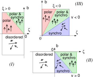
Figure 3: Phase diagram, in the plane $(\zeta,b)$: interplay between phase & orientation dynamics. We discuss 3 important cases. $(I)$ Polar order promotes the transition to synchronisation in region which is forbidden if they are decoupled provided $\xi>0$. $(II)$ Likewise, synchronisation promotes the transition to polar order in a region which is forbidden to the decoupled system, provided $v>0$. In both cases the region of both synchronisation $\&$ polar order is widened. $(III)$ The opposite situation arises when $\xi,v<0$: there synchronisation inhibits the transition to polar order; similarly, the polar order works against synchronisation. As a result the region with both synchronisation and polar order is reduced compared to the uncoupled system. Other intermediate cases are also possible.

Hydrodynamic modes & stability of bulk states

Broken symmetry states have slow dynamics of their soft modes. A full description involves studying $2d-1$ modes in $d$-dimensions so we restrict ourselves to one illustrative case. A state with macroscopic fixed polarity $\mathbf{P},{\bm{\Pi}}$ and synchronisation $\mathbf{\Phi}_{0}$ (with ${\bm{\Pi}}\neq\Phi_{0}\mathbf{P}$). We choose w.l.g the phases of $\Phi_{0},{\bm{\Pi}}$ to be zero and explore the soft modes associated with synchronisation alone, $\mathbf{\Phi}({\bf r},t)=\mathbf{\Phi}_{0}e^{i\phi({\bf r},t)}$. We consider a collection of nonlinear oscillating force dipoles with frequency $\omega$, amplitude $A$ and friction coefficient $\gamma$ suspended in an incompressible viscous fluid in creeping flow. In this oscillating state, the fluid velocity, ${\bf v}({\bf r},t)=\sum_{n=0}^{\infty}{\bf v}^{(n)}({\bf r})\sin(2\omega nt+2\phi_{n}({\bf r}))$ by the Floquet-Bloch theorem. The local phase dynamics is governed by (${\bf v}^{(n)}=0,n\neq 2$) Marchetti et al. (2013); Leoni and Liverpool (2012)

$$\eta\nabla^{2}{\bf v}({\bf r},t)-\nabla p=\nabla\cdot\bm{\sigma}^{a}\;;\;\nabla\cdot{\bf v}=0$$ (5)

$${\cal D}_{t}\phi+P_{i}\omega_{ij}\Pi_{j}=\lambda P_{i}u_{ij}\Pi_{j}+\lambda^{\prime}P_{i}u_{ij}P_{j}+D_{\phi}\nabla^{2}\phi$$ (6)

where ${\cal D}_{t}g({\bf r},t)=\partial_{t}g+(\mathbf{v}+\beta\mathbf{P}+\beta^{\prime}{\bm{\Pi}})\cdot\nabla g$, $\omega_{ij}=\frac{1}{2}(\partial_{i}v_{j}-\partial_{j}v_{i})$ and $u_{ij}=\frac{1}{2}(\partial_{i}v_{j}+\partial_{j}v_{i})$. The oscillating active stress, $\mathbf{\sigma}^{a}_{ij}(t)=P_{i}P_{j}\left(\alpha+\frac{1}{2}A^{2}\rho\gamma\omega\sin(2\omega t+2\phi)\right)$ implies $\phi=\phi_{2}$, and $\alpha=\bar{\sf Fd}$ is the average force dipole Leoni and Liverpool (2012). An instructive case has $\mathbf{P}=P\,\hat{\bm{z}}$ and ${\bm{\Pi}}=\Pi\,\hat{\bm{x}}$. With units s.t. $P=\Pi=1$, a linearized analysis of these equations then reveals modes $\phi_{\bf k}(t)=\int_{r}\phi({\bf r},t)e^{i{\bf k}\cdot{\bf r}},{\bf v}_{\bf k}(t)=\int_{r}{\bf v}^{(2)}({\bf r},t)e^{i{\bf k}\cdot{\bf r}}$ which relax as $\phi_{\bf k}(t)=\phi_{\bf k}(0)e^{-t/\tau_{\phi}(k)},{\bf v}_{\bf k}(t)={\bf v}_{\bf k}(0)e^{-t/\tau_{v}(k)}$, where $\tau_{v}^{-1}(k)=\tau_{\phi}^{-1}(k)=i\beta k_{z}+i\beta^{\prime}k_{x}+D_{\phi}k^{2}+\Lambda(k)$, with $\Lambda(k)=\alpha^{\prime}\left(\hat{k}_{x}\hat{k}_{z}(1+\lambda(1-2\hat{k}_{z}^{2}))+2\lambda^{\prime}\hat{k}_{z}^{2}(1-\hat{k}_{z}^{2})\right)$ where $\hat{k}_{i}=k_{i}/|{\bf k}|$ and $\alpha^{\prime}=\frac{1}{2\eta}A^{2}\rho\gamma\omega$. The synchronised state has a long wavelength instability to propagating phase fluctuations reminiscent of metachronal waves Yi et al. (2003). It is interesting that the propagation direction is intermediate between ${\bm{\Pi}}$ and $\mathbf{P}$, as metachronal waves tend to propagate at an angle to the beating direction Yi et al. (2003).

Microscopics

A microscopic picture of the system is provided by a dilute collection of micro-swimmers, for simplicity confined to a plane. A minimal swimmer has an oscillating force dipole in an incompressible, three-dimensional fluid (velocity ${\bf v}({\bf r},t)$) of viscosity $\eta$ and Re=0. A concrete example is given by the three-bead swimmer Najafi and Golestanian (2004). The swimmer with centre of mass at ${\bf r}$, oriented along $\hat{\bm{u}}$, is made up of three collinear spheres, of radius $\mathfrak{a}$, with coordinates $x_{1},x_{2},x_{3}$ and linked together by extensible links with negligible effect on the fluid. The spheres are subject to collinear forces $f_{1},f_{2},f_{3}$ with $f_{1}+f_{2}+f_{3}=0$ (force-free). The links, $L_{j}:=x_{j+1}-x_{j}$, for $j=1,2$, have dynamics $L_{j}=l_{i}+d_{j}(t)$ where $d_{j}(t)$ represent the swimming stroke. The forces and displacements are related by $\dot{d}_{i}=\frac{1}{\gamma}F_{i}+{\hat{\bm{u}}}\cdot({\bf v}({\bf r},t)-\dot{\bf r}),\;i=1,2$ with $\gamma=6\pi\eta\mathfrak{a}$ and $F_{1}=-[2f_{1}+f_{3}]\equiv{\sf F}$, $F_{2}:=[f_{1}+2f_{3}]$ ($d_{1}\equiv{\sf d}$). The force ${\sf F}$ evolves according to Leoni and Liverpool (2012)

$${d{\sf F}}/{dt}=-{k}{\sf d}/{\tau}+\mu(1-\sigma{\sf d}^{2}){\sf F}/{\gamma}+\alpha{\sf d}^{3}\;,$$ (7)

leading to spontaneous oscillations. To study the dynamics of ${\sf d}(t)$ we introduce a complex amplitude $A=Re^{i\varphi}$, ${\sf d}(t)=\frac{1}{2}[Ae^{i\omega t}+A^{*}e^{-i\omega t}]\Rightarrow$ $\dot{\sf d}(t)=\frac{i\omega}{2}[Ae^{i\omega t}-A^{*}e^{-i\omega t}]$. $R,\varphi\in\mathbb{R}^{1}$ are the amplitude, phase of the oscillations. $d_{2}(t)$ is a prescribed function of time: $d_{2}(t)=d\sin(\omega t+\varphi)$, and $\dot{F}_{2}\approx\gamma\ddot{d}_{2}(t)$. By averaging over the fast oscillation period $T=2\pi\omega^{-1}$ we obtain an effective description Leoni and Liverpool (2010b, a, 2012) in terms of the orientation $\hat{\bm{u}}$, phase $\varphi$ and amplitude $R$. Next we eliminate the amplitude $R$ keeping only the slower phase $\varphi$ Leoni and Liverpool (2012) and hence define $\mathbf{X}\equiv(\hat{\bm{u}},\varphi,{\bf r})$. We consider $N$ such objects characterised by $\mathbf{X}_{k}(t)$. To obtain averages we use the one-particle concentration $c(\mathbf{X},t):=\langle N^{-1}\sum^{N}_{k=1}\delta(\mathbf{X}-\mathbf{X}_{k}(t))\rangle$, the density of elements with $\mathbf{X}$ at time $t$. Performing averages over $c$ Ahmadi et al. (2006), we can obtain the quantities $\Phi({\bf r},t)$, $\mathbf{P}({\bf r},t)$ and $\bm{\Pi}({\bf r},t)$ introduced above. For this model both $v>0$ and $\xi>0$, when $R\gg d$.

In conclusion, we have extended the study of active systems to include collections of orientable units with an internal cycle characterised by a single phase variable. These show two different types of order: synchronisation where the individual phases are correlated and liquid crystalline order where their orientations are correlated. We derived phenomenological equations describing the dynamics of a spatially homogeneous mixture with hydrodynamic interactions, focussing on the interplay of phase and orientation. Our study reveals that each type of order can promote the transition to a state where both types of order are present, in a region of the parameters space that would be inaccessible if the two dynamics were decoupled. This is supported by a microscopic model of swimmers able to synchronise. From the theoretical point of view, the symmetry breaking associated with the synchronisation transition presents analogies with the physical mechanism yielding the Meissner effect in superconductivity or the Higgs mechanism in particle physics. A natural future direction is a complete description of the coupled hydrodynamic modes.

We thank S. Fürthauer and S. Ramaswamy for sharing a manuscript on a related topic and acknowledge the support of the EPSRC No. Grant EP/G026440/1.

References

- Marchetti et al. (2013) M. C. Marchetti et al., Rev. Mod. Phys. 85, 1143 (2013).
- Lauga and Powers (2009) E. Lauga and T. R. Powers, Rep. Prog. Phys. 72, 096601 (2009).
- Toner and Tu (1995) J. Toner and Y. Tu, Phys. Rev. Lett. 75, 4326 (1995).
- Aditi Simha and Ramaswamy (2002) R. Aditi Simha and S. Ramaswamy, Phys. Rev. Lett. 89, 058101 (2002).
- Kruse et al. (2005) K. Kruse et al., Eur. Phys. J E 16, 5 (2005).
- Ahmadi et al. (2006) A. Ahmadi, M. C. Marchetti, and T. B. Liverpool, Phys. Rev. E 74, 061913 (2006).
- Sachs (1991) T. Sachs, Pattern Formation in Plant Tissues. (Cambridge University Press, 1991).
- Sokolov and Aranson (2009) A. Sokolov and I. S. Aranson, Phys. Rev. Lett. 103, 148101 (2009).
- Rafai et al. (2010) S. Rafai, L. Jibuti, and P. Peyla, Phys. Rev. Lett. 104, 098102 (2010).
- Sokolov et al. (2007) A. Sokolov et al., Phys. Rev. Lett. 98, 158102 (2007).
- Riedel et al. (2005) I. H. Riedel, K. Kruse, and J. Howard, Science 309, 300 (2005).
- Dombrowski et al. (2004) C. Dombrowski et al., Phys. Rev. Lett. 93, 098103 (2004).
- Saintillan and Shelley (2008) D. Saintillan and M. J. Shelley, Physics of Fluids 20, 123304 (2008).
- Baskaran and Marchetti (2009) A. Baskaran and M. C. Marchetti, PNAS 106, 15567 (2009).
- Ginelli et al. (2010) F. Ginelli, F. Peruani, M. Bar, and H. Chaté, Phys. Rev. Lett. 104, 184502 (2010).
- Leoni and Liverpool (2010a) M. Leoni and T. B. Liverpool, Phys Rev Lett 105, 238102 (2010a).
- Taylor (1951) G. Taylor, Proc. R. Soc. Lond. A 209, 447 (1951).
- Guirao and Joanny (2007) B. Guirao and J. F. Joanny, Biophys. J. 92, 1900 (2007).
- Polin et al. (2009) M. Polin et al., Science 325, 487 (2009).
- Goldstein et al. (2009) R. E. Goldstein, M. Polin, and I. Tuval, Phys. Rev. Lett. 103, 168103 (2009).
- Sanchez et al. (2011) T. Sanchez et al., Science 333, 456 (2011).
- Kotar et al. (2010) J. Kotar et al., PNAS 107, 7669 (2010).
- Qian et al. (2009) B. Qian et al., Phys. Rev. E 80, 061919 (2009).
- Kim and Powers (2004) M. Kim and T. R. Powers, Phys. Rev. E 69, 061910 (2004).
- Reichert and Stark (2005) M. Reichert and H. Stark, Eur. Phys. J E (2005).
- Vilfan and Julicher (2006) A. Vilfan and F. Julicher, Phys. Rev. Lett. 96, 058102 (2006).
- Niedermayer et al. (2008) T. Niedermayer, B. Eckhardt, and P. Lenz, Chaos 18, 037128 (2008).
- Uchida and Golestanian (2010) N. Uchida and R. Golestanian, Phys. Rev. Lett. 104, 178103 (2010).
- Leoni and Liverpool (2012) M. Leoni and T. B. Liverpool, Phys. Rev. E 85, 040901(R) (2012).
- de Gennes and Prost (1995) P. G. de Gennes and J. Prost, The physics of liquid crystals (Oxford University Press, 1995).
- Leoni and Liverpool (2013) M. Leoni and T. Liverpool, unpublished (2013).
- Acebrón et al. (2005) J. A. Acebrón et al., Rev. Mod. Phys. 77, 137 (2005).
- Note (1) On the limit cycle, oscillations are called non-isochronous if the frequency depends on the amplitude of the oscillations.
- Note (2) If there are correlations such that flipping the orientation corresponds to a phase shift these two cases would be identical. This happens for force monopoles.
- Yi et al. (2003) W.-J. Yi, K.-S. Park, C.-H. Lee, and C.-S. Rhee, Med. Biol. Eng. Comput 41, 481 (2003).
- Najafi and Golestanian (2004) A. Najafi and R. Golestanian, Phys Rev E Stat Nonlin Soft Matter Phys 69, 062901 (2004).
- Leoni and Liverpool (2010b) M. Leoni and T. B. Liverpool, Europhys. Lett 92, 64004 (2010b).