Goldstone modes and bifurcations in phase-separated binary condensates at finite temperature

Abstract

We show that the third Goldstone mode, which emerges in binary condensates at phase-separation, persists to higher inter-species interaction for density profiles where one component is surrounded on both sides by the other component. This is not the case with symmetry-broken density profiles where one species is to entirely to the left and the other is entirely to the right. We, then, use Hartree-Fock-Bogoliubov theory with Popov approximation to examine the mode evolution at $\displaystyle T\neq 0$ and demonstrate the existence of mode bifurcation near the critical temperature. The Kohn mode, however, exhibits deviation from the natural frequency at finite temperatures after the phase separation. This is due to the exclusion of the non-condensate atoms in the dynamics.

I Introduction

The remarkable feature of binary condensates or two-species Bose-Einstein condensates (TBECs) is the phenomenon of phase separation Ho and Shenoy (1996); Trippenbach et al. (2000). This relates the system to novel phenomena in nonlinear dynamics and pattern formation, non-equilibrium statistical mechanics, optical systems and phase transitions in condensed matter systems. Experimentally, TBECs have been realized in the mixture of two different alkali atoms Modugno et al. (2002); Lercher et al. (2011); McCarron et al. (2011), and in two different isotopes Inouye et al. (1998) and hyperfine states Stamper-Kurn et al. (1998); Myatt et al. (1997) of an atom. Most importantly, in experiments, the TBEC can be steered from miscible to phase-separated domain or vice-versa Papp et al. (2008); Tojo et al. (2010) through a Feshbach resonance. These have motivated theoretical investigations on stationary states Ho and Shenoy (1996); Gautam and Angom (2011), dynamical instabilities Sasaki et al. (2009); Gautam and Angom (2010); Kadokura et al. (2012) and collective excitations Stringari (1996); Pu and Bigelow (1998); Graham and Walls (1998); Gordon and Savage (1998); Kuopanportti et al. (2012); Ticknor (2013); Takeuchi and Kasamatsu (2013)of TBECs.

In this paper, we report the development of Hartree-Fock-Bogoliubov theory with Popov (HFB-Popov) approximation Griffin (1996) for TBECs. We use it to investigate the evolution of Goldstone modes and mode energies as function of the inter-species interaction and temperature, respectively. Recent works Ticknor (2013); Takeuchi and Kasamatsu (2013) reported the existence of an additional Goldstone mode at phase separation in the symmetry-broken density profiles, which we refer to as the side-by-side density profiles. We, however, demonstrate that in the other type of density profile where one of the species is surrounded on both sides by the other, which we refer to as the sandwich type, the mode evolves very differently. To include the finite temperature effects, besides HFB-Popov approximation, there are other different approaches. These include projected Gross-Pitaevskii (GP) equation Blakie et al. (2008), stochastic GP equation(SGPE)Proukakis and Jackson (2008) and Zaremba-Nikuni-Griffin(ZNG) formalism Zaremba et al. (1999). For the present work we have chosen the HFB-Popov approximation, which is a gapless theory and satisfies the Hugenholtz-Pines theorem Hugenholtz and Pines (1959). The method is particularly well suited to examine the evolution of the low-lying modes. It has been used extensively in single species BEC to study finite temperature effects to mode energies Griffin (1996); Hutchinson et al. (1997); Dodd et al. (1998); Gies et al. (2004) and agrees well with the experimental results Jin et al. (1997) at low temperatures. In TBECs, the HFB-Popov approximation has been used in the miscible domain Pires and de Passos (2008) and in this paper, we describe the results for the phase-separated domain. Other works which have examined the finite temperature effects in TBECs use Hartree-Fock treatment with or without trapping potential Öhberg and Stenholm (1998); Zhang and Fertig (2007) and semi-classical approach Öhberg (1999). Although, HFB-Popov does have the advantage vis-a-vis calculation of the modes, it is nontrivial to get converged solutions. In the present work, we consider the TBEC of ⁸⁷Rb-¹³³Cs Lercher et al. (2011); McCarron et al. (2011), which have widely differing $\displaystyle s$-wave scattering lengths and masses. This choice does add to the severity of the convergence issues but this also makes it a good test for the methods we use. We choose the parameter domain where the system is quasi-1D and a mean-field description like HFB-Popov is applicable. The quasi-1D trapped bosons exhibit a rich phase structure as a function of density and interaction strengths Petrov et al. (2000). For comparison with the experimental results we also consider the parameters as in the experiment McCarron et al. (2011). We find that, like in Ref. Egorov et al. (2013), the quasi-1D description are in good agreement with the condensate density profiles of 3D calculations Pattinson et al. (2013).

II Theory

For a highly anisotropic cigar shaped harmonic trapping potential $\displaystyle(1/2)m(\omega_{x}^{2}x^{2}+\omega_{y}^{2}y^{2}+\omega_{z}^{2}z^{2})$, with $\displaystyle\omega_{x}=\omega_{y}=\omega_{\perp}\gg\omega_{z}$. In this case, we can integrate out the condensate wave function along $\displaystyle xy$ and reduce it to a quasi-1D system. The transverse degrees of freedom are then frozen and the system is confined in the harmonic oscillator ground state along the transverse direction for which $\displaystyle\hbar\omega_{\perp}\gg\mu_{k}$. We thus consider excitations present only in the axial direction $\displaystyle z$ Mateo and Delgado (2008, 2009). The grand-canonical Hamiltonian, in the second quantized form, describing the mixture of two interacting BECs is then

$$\displaystyle H \displaystyle= \displaystyle\sum_{k=1,2}\int dz\hat{\Psi}_{k}^{\dagger}(z,t)\bigg{[}-\frac{\hbar^{2}}{2m_{k}}\frac{\partial^{2}}{\partial z^{2}}+V_{k}(z)-\mu_{k}$$ (1)

$$\displaystyle+\frac{U_{kk}}{2}\hat{\Psi}_{k}^{\dagger}(z,t)\hat{\Psi}_{k}(z,t)\bigg{]}\hat{\Psi}_{k}(z,t)$$

$$\displaystyle+U_{12}\int dz\hat{\Psi}_{1}^{\dagger}(z,t)\hat{\Psi}_{2}^{\dagger}(z,t)\hat{\Psi}_{1}(z,t)\hat{\Psi}_{2}(z,t),$$

where $\displaystyle k=1,2$ is the species index, $\displaystyle\hat{\Psi}_{k}$’s are the Bose field operators of the two different species, and $\displaystyle\mu_{k}$’s are the chemical potentials. The strength of intra and inter-species interactions are $\displaystyle U_{kk}=(a_{kk}\lambda)/m_{k}$ and $\displaystyle U_{12}=(a_{12}\lambda)/(2m_{12})$, respectively, where $\displaystyle\lambda=(\omega_{\perp}/\omega_{z})\gg 1$ is the anisotropy parameter, $\displaystyle a_{kk}$ is the $\displaystyle s$-wave scattering length, $\displaystyle m_{k}$’s are the atomic masses of the species and $\displaystyle m_{12}=m_{1}m_{2}/(m_{1}+m_{2})$. In the present work we consider all the interactions are repulsive, that is $\displaystyle a_{kk},a_{12}>0$. The equation of motion of the Bose field operators is

$$i\hbar\frac{\partial}{\partial t}\begin{pmatrix}\hat{\Psi}_{1}\\ \hat{\Psi}_{2}\end{pmatrix}\!\!=\!\!\begin{pmatrix}\hat{h}_{1}+U_{11}\hat{\Psi}_{1}^{\dagger}\hat{\Psi}_{1}&U_{12}\hat{\Psi}_{2}^{\dagger}\hat{\Psi}_{1}\\ U_{12}\hat{\Psi}_{1}^{\dagger}\hat{\Psi}_{2}&\hat{h}_{2}+U_{22}\hat{\Psi}_{2}^{\dagger}\hat{\Psi}_{2}\end{pmatrix}\!\!\!\begin{pmatrix}\hat{\Psi}_{1}\\ \hat{\Psi}_{2}\end{pmatrix}$$

where $\displaystyle\hat{h}_{k}=(-\hbar^{2}/2m_{k})\partial^{2}/\partial z^{2}+V_{k}(z)-\mu_{k}$. For compact notations, we refrain from writing the explicit dependence of $\displaystyle\hat{\Psi}_{k}$ on $\displaystyle z$ and $\displaystyle t$. Since a majority of the atoms reside in the ground state for the temperature regime relevant to the experiments ($\displaystyle T\leqslant 0.65T_{c}$ ) Dodd et al. (1998), the condensate part can be separated out from the Bose field operator $\displaystyle\hat{\Psi}({\mathbf{r}},t)$. The non-condensed or the thermal cloud of atoms are then the fluctuations of the condensate field. Here, $\displaystyle T_{c}$ is the critical temperature of ideal gas in a harmonic confining potential. Accordingly, we define Griffin (1996), $\displaystyle\hat{\Psi}(z,t)=\Phi(z)+\tilde{\Psi}(z,t)$, where $\displaystyle\Phi(z)$ is a $\displaystyle c$-field and represents the condensate, and $\displaystyle\tilde{\Psi}(z,t)$ is the fluctuation part. In two component representation

$$\displaystyle\begin{pmatrix}\hat{\Psi}_{1}\\ \hat{\Psi}_{2}\end{pmatrix}=\begin{pmatrix}\phi_{1}\\ \phi_{2}\end{pmatrix}+\begin{pmatrix}\tilde{\psi}_{1}\\ \tilde{\psi}_{2}\\ \end{pmatrix},$$ (2)

where $\displaystyle\phi_{k}(z)$ and $\displaystyle\tilde{\psi}_{k}(z)$ are the condensate and fluctuation part of the $\displaystyle k$th species. Thus for a TBEC, $\displaystyle\phi_{k}$s are the static solutions of the coupled generalized GP equations, with time-independent HFB-Popov approximation, given by

$$\displaystyle\hat{h}_{1}\phi_{1}+U_{11}\left[n_{c1}+2\tilde{n}_{1}\right]\phi_{1}+U_{12}n_{2}\phi_{1}=0,$$ (3a)

$$\displaystyle\hat{h}_{2}\phi_{2}+U_{22}\left[n_{c2}+2\tilde{n}_{2}\right]\phi_{2}+U_{12}n_{1}\phi_{2}=0,$$ (3b)

where, $\displaystyle n_{ck}(z)\equiv|\phi_{k}(z)|^{2}$, $\displaystyle\tilde{n}_{k}(z)\equiv\langle\tilde{\psi}_{k}^{\dagger}(z,t)\tilde{\psi}_{k}(z,t)\rangle$, and $\displaystyle n_{k}(z)=n_{ck}(z)+\tilde{n}_{k}(z)$ are the local condensate, non-condensate, and total density, respectively. Using Bogoliubov transformation

$$\tilde{\psi}_{k}(z,t)=\sum_{j}\left[u_{kj}(z)\hat{\alpha}_{j}(z)e^{-iE_{j}t}-v_{kj}^{*}(z)\hat{\alpha}_{j}^{\dagger}(z)e^{iE_{j}t}\right],$$

where, $\displaystyle\hat{\alpha}_{j}$ ($\displaystyle\hat{\alpha}_{j}^{\dagger}$) are the quasi-particle annihilation (creation) operators and satisfy Bose commutation relations, $\displaystyle u_{k}$ and $\displaystyle v_{k}$ are the quasi-particle amplitudes, and $\displaystyle j$ is the energy eigenvalue index. We define the operators as common to both the species, which is natural and consistent as the dynamics of the species are coupled. Furthermore, this reproduces the standard coupled Bogoliubov-de Gennes equations at $\displaystyle T=0$ Ticknor (2013) and in the limit $\displaystyle a_{12}\rightarrow 0$, non-interacting TBEC, the quasi-particle spectra separates into two distinct sets: one set for each of the condensates. From the above definitions, we get the following Bogoliubov-de Gennes equations

$$\displaystyle\hat{{\mathcal{L}}}_{1}u_{1j}-U_{11}\phi_{1}^{2}v_{1j}+U_{12}\phi_{1}\left(\phi_{2}^{*}u_{2j}-\phi_{2}v_{2j}\right) \displaystyle= \displaystyle E_{j}u_{1j},\;\;\;\;\;\;$$ (4a)

$$\displaystyle\hat{\underline{\mathcal{L}}}_{1}v_{1j}+U_{11}\phi_{1}^{*2}u_{1j}-U_{12}\phi_{1}^{*}\left(\phi_{2}v_{2j}-\phi_{2}^{*}u_{2j}\right) \displaystyle= \displaystyle E_{j}v_{1j},\;\;\;\;\;\;$$ (4b)

$$\displaystyle\hat{{\mathcal{L}}}_{2}u_{2j}-U_{22}\phi_{2}^{2}v_{2j}+U_{12}\phi_{2}\left(\phi_{1}^{*}u_{1j}-\phi_{1}v_{1j}\right) \displaystyle= \displaystyle E_{j}u_{2j},\;\;\;\;\;\;$$ (4c)

$$\displaystyle\hat{\underline{\mathcal{L}}}_{2}v_{2j}+U_{22}\phi_{2}^{*2}u_{2j}-U_{12}\phi_{2}^{*}\left(\phi_{1}v_{1j}-\phi_{1}^{*}u_{1j}\right) \displaystyle= \displaystyle E_{j}v_{2j},\;\;\;\;\;\;$$ (4d)

where $\displaystyle\hat{{\mathcal{L}}}_{1}=\big{(}\hat{h}_{1}+2U_{11}n_{1}+U_{12}n_{2})$, $\displaystyle\hat{{\mathcal{L}}}_{2}=\big{(}\hat{h}_{2}+2U_{22}n_{2}+U_{12}n_{1}\big{)}$ and $\displaystyle\hat{\underline{\cal L}}_{k}=-\hat{\cal L}_{k}$. To solve Eq. (4) we define $\displaystyle u_{k}$ and $\displaystyle v_{k}$’s as linear combination of $\displaystyle N$ harmonic oscillator eigenstates.

$$\displaystyle u_{1j}=\sum_{i=0}^{N}p_{ij}\xi_{i},\;\;v_{1j}=\sum_{i=0}^{N}q_{ij}\xi_{i},$$

$$\displaystyle u_{2j}=\sum_{i=0}^{N}r_{ij}\xi_{i},\;\;v_{2j}=\sum_{i=0}^{N}s_{ij}\xi_{i},$$ (5)

where $\displaystyle\xi_{i}$ is the $\displaystyle i$th harmonic oscillator eigenstate and $\displaystyle p_{ij}$, $\displaystyle q_{ij}$, $\displaystyle r_{ij}$ and $\displaystyle s_{ij}$ are the coefficients of linear combination. Using this expansion the Eq. (4) is then reduced to a matrix eigenvalue equation and solved using standard matrix diagonalization algorithms. The matrix has a dimension of $\displaystyle 4N\times 4N$ and is non-Hermitian, non-symmetric and may have complex eigenvalues. In the present work, to avoid metastable states, we ensure that $\displaystyle E_{j}$’s are real during the iteration. The eigenvalue spectrum obtained from the diagonalization of the matrix has an equal number of positive and negative eigenvalues $\displaystyle E_{j}$’s. The number density $\displaystyle\tilde{n}_{k}$ of the non-condensate atoms is then

$$\tilde{n}_{k}=\sum_{j}\{[|u_{kj}|^{2}+|v_{kj}|^{2}]N_{0}(E_{j})+|v_{kj}|^{2}\},$$ (6)

where $\displaystyle\langle\hat{\alpha}_{j}^{\dagger}\hat{\alpha}_{j}\rangle=(e^{\beta E_{j}}-1)^{-1}\equiv N_{0}(E_{j})$ is the Bose factor of the quasi-particle state with real and positive energy $\displaystyle E_{j}$. The coupled Eqns. (3) and(4) are solved iteratively till the solutions converge to desired accuracy. However, it should be emphasized that, when $\displaystyle T\rightarrow 0$, $\displaystyle N_{0}(E_{j})$’s in Eq. (6) vanishes. The non-condensate density is then reduced to

$$\tilde{n}_{k}=\sum_{j}|v_{kj}|^{2}.$$ (7)

Thus, at zero temperature we need to solve the equations self-consistently as the quantum depletion term $\displaystyle|v_{kj}|^{2}$ in the above equation is non-zero. The contribution from the quantum depletion to the non-condensate is very small, it is $\displaystyle\approx 0.1\%$ for the set of parameters used in our calculations. In addition, the solutions to the equations converge in less than five iterations.

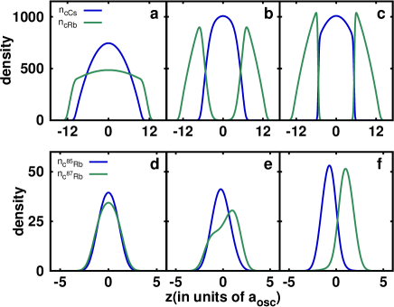
Figure 1: (Color online) Transition to phase separation and structure of the density profiles in TBEC. (a-c) show the transition from miscible to sandwich type density profile with the change in interspecies scattering length $\displaystyle a_{\rm CsRb}$ for a Cs-Rb TBEC and correspond to $\displaystyle a_{\rm CsRb}=\{200a_{0},310a_{0},420a_{0}\}$ respectively. The density profiles in (c) is referred to as the sandwich type. (d-f) show the transition from miscible to side-by-side density profile with the change in $\displaystyle a_{{}^{85}{\rm Rb}^{87}{\rm Rb}}$ for a ${}^{85}{\rm Rb}-^{87}{\rm Rb}$ TBEC and correspond to $\displaystyle a_{{}^{85}{\rm Rb}^{87}{\rm Rb}}=\{100a_{0},290a_{0},400a_{0}\}$ respectively. The density profile in (f) is referred to as the side-by-side type. In the plots density is measured in units of $\displaystyle a_{\rm osc}^{-1}$.

III Results and discussions

III.1 Numerical details

For the $\displaystyle T=0$ studies we solve the pair of coupled Eqs. (3) by neglecting the non-condensate density ($\displaystyle\tilde{n}_{k}=0$) using finite-difference methods and in particular, we use the split-step Crank-Nicholson method  Muruganandam and Adhikari (2009) adapted for binary condensates. The method when implemented with imaginary time propagation is appropriate to obtain the stationary ground state wave function of the TBEC. Using this solution, and based on Eq. (5), we cast the Eq. (4) as a matrix eigenvalue equation in the basis of the trapping potential. The matrix is then diagonalized using the LAPACK routine zgeev Anderson et al. (1999) to find the quasi-particle energies and amplitudes, $\displaystyle E_{j}$, and $\displaystyle u_{k}$’s and $\displaystyle v_{k}$’s, respectively. This step is the beginning of the first iteration for $\displaystyle T\neq 0$ calculations. In which case, the $\displaystyle u_{k}$’s and $\displaystyle v_{k}$’s along with $\displaystyle E_{j}$ are used to get the initial estimate of $\displaystyle\tilde{n}_{k}$ through Eq. (6). For this we consider only the positive energy modes. Using this updated value of $\displaystyle\tilde{n}_{k}$, the ground state wave function of TBEC $\displaystyle\phi_{k}$ and chemical potential $\displaystyle\mu_{k}$ are again re-calculated from Eq. (3). This procedure is repeated till the solutions reach desired convergence. In the present work the convergence criteria is that the change in $\displaystyle\mu_{k}$ between iterations should be less than $\displaystyle 10^{-4}$. In general, the convergence is not smooth and we encounter severe oscillations very frequently. To damp the oscillations and accelerate convergence we employ successive over (under) relaxation technique for updating the condensate (non-condensate) densitiesSimula et al. (2001). The new solutions after $\displaystyle{\rm IC}$ iteration cycle are

$$\displaystyle\phi_{\rm IC}^{\rm new}(z) \displaystyle= \displaystyle s^{\rm ov}\phi_{\rm IC}(z)+(1-s^{\rm ov})\phi_{\rm IC-1}(z),$$

$$\displaystyle\tilde{n}_{\rm IC}^{\rm new}(z) \displaystyle= \displaystyle s^{\rm un}\tilde{n}_{\rm IC}(z)+(1-s^{\rm un})\tilde{n}_{\rm IC-1}(z),$$ (8)

where $\displaystyle s^{\rm ov}>1$ ($\displaystyle s^{\rm un}<1$) is the over (under) relaxation parameter. During the calculation of the $\displaystyle u_{k}$ and $\displaystyle v_{k}$, we choose an optimal number of the harmonic oscillator basis functions. The conditions based on which we decide the optimal size are: obtaining reliable Goldstone modes; and all eigen values must be real. For the $\displaystyle T=0$ studies we find that a basis set consisting of 130 harmonic oscillator eigenstates is an optimal choice. We observe the Goldstone modes eigenenergies becoming complex, with a small imaginary component, in the eigen spectrum when the basis set is very large. So, in the present studies, we ensure that there are no complex eigenvalues with an appropriate choice of the basis set size.

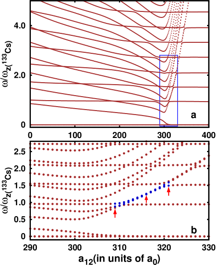
Figure 2: (Color online) The evolution of the modes as a function of the interspecies scattering length $\displaystyle a_{\rm CsRb}$ in Cs-Rb TBEC. (a) shows the evolution of the low-lying modes in the domain $\displaystyle 0\leqslant a_{\rm CsRb}\leqslant 400a_{0}$ for $\displaystyle N_{{}^{87}{\rm Rb}}=N_{{}^{133}{\rm Cs}}=10^{4}$. (b) is the enlarged view of the region enclosed within the blue colored rectangular box in figure (a) to resolve the avoided crossing and quasi-degeneracy of modes (highlighted with dark-blue points). The points marked with red arrows corresponds to interspecies scattering length $\displaystyle a_{\rm CsRb}=\{309a_{0},316a_{0},321a_{0}\}$ respectively.

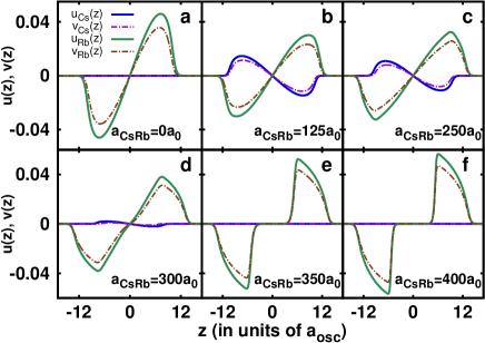
Figure 3: (Color online) Evolution of quasi-particle amplitude corresponding to the Rb Kohn mode as $\displaystyle a_{{}_{\rm CsRb}}$ is increased from 0 to 400$\displaystyle a_{0}$. For better visibility $\displaystyle u_{\rm cs}$ and $\displaystyle u_{\rm Rb}$ are scaled by a factor of 1.2. (a) When $\displaystyle a_{{}_{\rm CsRb}}=0$, it is a Kohn mode of the Rb condensate. (b-d) In the domain $\displaystyle 0<a_{{}_{\rm CsRb}}\lesssim 310a_{0}$ the mode acquires admixtures from the Cs Kohn mode (nonzero $\displaystyle u_{\rm Cs}$ and $\displaystyle v_{\rm Cs}$). (e-f) At phase separation $\displaystyle 310a_{0}\lesssim a_{{}_{\rm CsRb}}$ the mode transforms to a Goldstone mode: $\displaystyle u_{\rm Rb}$ and $\displaystyle v_{\rm Rb}$ have same profile as the $\displaystyle n_{\rm Rb}=|\phi_{\rm Rb}|^{2}$ but with a phase difference. In the plots $\displaystyle u$’s and $\displaystyle v$’s are in units of $\displaystyle a_{\rm osc}^{-1/2}$.

III.2 Mode evolution of trapped TBEC at $\displaystyle T=0$

In TBECs, phase separation occurs when $\displaystyle U_{12}>\sqrt{U_{11}U_{22}}$. For the present work, we consider Cs and Rb as the first and second species, respectively. With this identification $\displaystyle a_{11}=a_{\rm CsCs}=280a_{0}$ and $\displaystyle a_{22}=a_{\rm RbRb}=100a_{0}$, where $\displaystyle a_{0}$ is the Bohr radius, and arrive at the condition for phase separation $\displaystyle a_{12}=a_{{}_{\rm CsRb}}>261a_{0}$, which is smaller than the background value of $\displaystyle a_{{}_{\rm CsRb}}\approx 650a_{0}$ Lercher et al. (2011). To examine the nature of modes in the neighbourhood of phase separation, we compute $\displaystyle E_{j}$ at $\displaystyle T=0$ and vary $\displaystyle a_{{}_{\rm CsRb}}$, which is experimentally possible with the Rb-Cs Feshbach resonance Pilch et al. (2009). The evolution of the low-lying modes in the domain $\displaystyle 0\leqslant a_{{}_{\rm CsRb}}\leqslant 450a_{0}$ with $\displaystyle N_{\rm Rb}=N_{\rm Cs}=10^{4}$ are computed with $\displaystyle\omega_{z({\rm Rb})}=2\pi\times 3.89$Hz and $\displaystyle\omega_{z({\rm Cs})}=2\pi\times 4.55$Hz as in ref. McCarron et al. (2011); Pattinson et al. (2013). However, to form a quasi-1D system we take $\displaystyle\omega_{\perp}=50\omega_{z}$, so that $\displaystyle\hbar\omega_{\perp}\gg\mu_{k}$. For these values, the relevant quasi-1D parameters $\displaystyle\alpha=2a_{{}_{\rm CsCs}}\sqrt{(\omega_{\perp}/\omega_{z})(m\omega_{\perp}/\hbar)}\approx 0.36$ and $\displaystyle\gamma=2(a_{{}_{\rm CsCs}}/n_{\rm Cs})(m\omega_{\perp}/\hbar)\approx 10^{-5}$, so the system is in the weakly interacting TF regime Petrov et al. (2000) and mean field description through GP-equation is valid. For this set of parameters the ground state is of sandwich geometry, in which the species with the heavier mass is at the center and flanked by the species with lighter mass at the edges. An example of the sandwich profile corresponding to the experimentally relevant parameters is shown in Fig (1)(c). On the other hand for TBEC with species of equal or near equal masses and low number of atoms, in general, the ground state geometry is side-by-side. As an example the side-by-side ground state density profile of ⁸⁵Rb-⁸⁷Rb TBEC is shown in Fig.  (1)(f).

From here on we consider the same set of $\displaystyle\omega_{z}$ ($\displaystyle\omega_{z({\rm Rb})}=2\pi\times 3.89$Hz and $\displaystyle\omega_{z({\rm Cs})}=2\pi\times 4.55$Hz ), as mentioned earlier, in the rest of the calculations reported in the manuscript. In the computations we scale the spatial and temporal variables as $\displaystyle z/a_{\rm osc(Cs)}$ and $\displaystyle\omega_{z({\rm Cs})}t$ which render the equations dimensionless. When $\displaystyle a_{{}_{\rm CsRb}}=0$, the $\displaystyle U_{\rm CsRb}$ dependent terms in Eq.(4) are zero and the spectrum of the two species are independent as the two condensates are decoupled. The system has two Goldstone modes, one each for the two species. The two lowest modes with nonzero excitation energies are the Kohn modes of the two species, and these occur at $\displaystyle\hbar\omega_{z({\rm Cs})}$ and $\displaystyle 0.85\hbar\omega_{z({\rm Cs})}$ for Cs and Rb species, respectively.

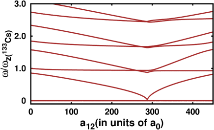
Figure 4: (Color online) Low-lying modes of ⁸⁵Rb-⁸⁷Rb for $\displaystyle N_{{}^{87}{\rm Rb}}=N_{{}^{85}{\rm Rb}}=10^{2}$ as a function of $\displaystyle a_{{}^{85}{\rm Rb}^{87}{\rm Rb}}$. At phase separation the structure of the density profiles is side-by-side and one of the modes goes soft.

III.2.1 Third Goldstone mode

The clear separation between the modes of the two species is lost and mode mixing occurs when $\displaystyle a_{{}_{\rm CsRb}}>0$. For example, the Kohn modes of the two species intermix when $\displaystyle a_{{}_{\rm CsRb}}>0$, however, there is a difference in the evolution of the mode energies. The energy of the Rb Kohn mode decreases, but the one corresponding to Cs remains steady at $\displaystyle\hbar\omega_{z({\rm Cs})}$. At higher $\displaystyle a_{{}_{\rm CsRb}}$ the energy of the Rb Kohn mode decreases further and goes soft at phase separation ($\displaystyle U_{\rm CsRb}>\sqrt{U_{\rm CsCs}U_{\rm RbRb}}$) when $\displaystyle a_{{}_{\rm CsRb}}\approx 310a_{0}$. This introduces a new Goldstone mode of the Rb BEC to the excitation spectrum. The reason is, for the parameters chosen, the density profiles at phase separation assume sandwich geometry with Cs BEC at the center and Rb BEC at the edges. So, the Rb BECs at the edges are effectively two topologically distinct BECs and there are two Goldstone modes with the same $\displaystyle|u_{\rm Rb}|$ and $\displaystyle|v_{\rm Rb}|$ but different phases. A similar result of the Kohn mode going soft was observed for single species BEC confined in a double well potential Salasnich et al. (1999). Although, the the two systems are widely different, there is a common genesis to the softening of the Kohn mode, and that is the partition of the one condensate cloud into two distinct ones. This could be, in our case by another condensate or by a potential barrier as in ref. Salasnich et al. (1999).

To examine the mode evolution with the experimentally realized parameters McCarron et al. (2011), we repeat the computations with $\displaystyle\omega_{\perp({\rm Cs})}=2\pi\times 40.2$Hz and $\displaystyle\omega_{\perp({\rm Rb})}=2\pi\times 32.2$Hz. With these parameters the system is not strictly quasi-1D as $\displaystyle\hbar\omega_{\perp k}\approx\mu_{k}$ for $\displaystyle N_{\rm Cs}=N_{\rm Rb}=10^{4}$, however, as $\displaystyle\omega_{zk}\ll\omega_{\perp k}$ there must be qualitative similarities to a quasi-1D system Egorov et al. (2013). Indeed, with the variation of $\displaystyle a_{{}_{\rm CsRb}}$ the modes evolve similar to the case of $\displaystyle\omega_{\perp k}=50\omega_{zk}$ and low-lying $\displaystyle\omega$s are shown in Fig. 2(a). The evolution of the Rb Kohn mode functions ($\displaystyle u_{\rm Rb}$ and $\displaystyle v_{\rm Rb}$) with $\displaystyle a_{{}_{\rm CsRb}}$ are shown in Fig. 3. It is evident that when $\displaystyle a_{{}_{\rm CsRb}}=0$ (Fig. 3(a)), there is no admixture from the Cs Kohn mode ( $\displaystyle u_{\rm Cs}=v_{\rm Cs}=0$). However, when $\displaystyle 0<a_{{}_{\rm CsRb}}\lesssim 310a_{0}$ the admixture from the Cs Kohn mode increases initially and then goes to zero as we approach $\displaystyle U_{\rm CsRb}>\sqrt{U_{\rm CsCs}U_{\rm RbRb}}$ (Fig. 3(b-f) ).

One striking result is, the Rb Kohn mode after going soft at $\displaystyle a_{{}_{\rm CsRb}}\approx 310a_{0}$, as shown in Fig. 2(a), continues as the third Goldstone mode for $\displaystyle 310a_{0}<a_{{}_{\rm CsRb}}$. This is different from the evolution of the zero energy mode in TBEC with side-by-side density profiles. In this case after phase separation, $\displaystyle z$-parity symmetry of the system is broken and the zero energy mode regains energy. So, there are only two Goldstone modes in the system. This is evident from Fig. 4, where we show the mode evolution of ⁸⁵Rb-⁸⁷Rb mixture with side-by-side density profiles at phase separation. The parameters of the system considered are $\displaystyle N_{{}^{85}{\rm Rb}}=N_{{}^{87}{\rm Rb}}=10^{2}$ with the same $\displaystyle\omega_{zk}$ and $\displaystyle\omega_{\perp k}$ as in the Rb-Cs mixture. Here, we use intra-species scattering lengths as $\displaystyle 99a_{0}$ and $\displaystyle 100a_{0}$ for ⁸⁵Rb and ⁸⁷Rb, respectively and tune the inter-species interaction for better comparison with the Rb-Cs results. This is, however, different from the experimental realization Papp et al. (2008), where the intra-species interaction of ⁸⁵Rb is varied. A similar result was reported in an earlier work on quasi-2D system of TBEC Ticknor (2013).

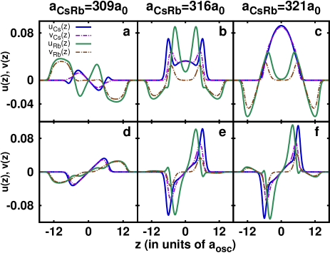
Figure 5: (Color online) The quasi-particle amplitudes of the 5th and 6th modes at quasi-degeneracy. (a-c) The quasi-particle amplitudes $\displaystyle u_{k}$’s and $\displaystyle v_{k}$’s of the $\displaystyle 5^{\rm th}$ mode for 3 values of $\displaystyle a_{{}_{\rm CsRb}}$ represented and marked by blue points and red arrows, respectively, in Fig. (2). (d-f) The quasi-particle amplitudes $\displaystyle u_{k}$’s and $\displaystyle v_{k}$’s corresponding to the $\displaystyle 6^{\rm th}$ mode for the same values of $\displaystyle a_{{}_{\rm CsRb}}$. In the plots $\displaystyle u_{k}$’s and $\displaystyle v_{k}$’s are in the units of $\displaystyle a_{\rm osc}^{-1/2}$.

III.2.2 Avoided crossings and quasi-degeneracy

From Fig. 2(a), it is evident that there are several instances of avoided level crossings as $\displaystyle a_{{}_{\rm CsRb}}$ is varied to higher values. These arise from the changes in the profile of $\displaystyle n_{ck}(z)$, the condensate densities, as the $\displaystyle u_{k}$ and $\displaystyle v_{k}$ depend on $\displaystyle n_{ck}(z)$ through the BdG equations. For this reason, the number of avoided crossings is high around the critical value of $\displaystyle a_{{}_{\rm CsRb}}$, where there is a significant change in the structure of $\displaystyle n_{ck}(z)$ due to phase separation. Another remarkable feature which emerges when $\displaystyle a_{{}_{\rm CsRb}}>310a_{0}$ are the avoided crossings involving three modes. As an example, the mode evolution around one such case involving the Kohn mode is shown in Fig. 2(b). Let us, in particular, examine the 5th and 6th modes, the corresponding mode energies in the domain of interest ($\displaystyle 309a_{0}\leqslant a_{{}_{\rm CsRb}}\leqslant 321a_{0}$) are represented by blue colored points in Fig. 2(b). At $\displaystyle a_{{}_{\rm CsRb}}=309a_{0}$, the 6th mode is the Kohn mode, which is evident from the dipolar structure of the $\displaystyle u_{k}$ and $\displaystyle v_{k}$ as shown in Fig. 5(d). The closest approach of the three modes, 4th, 5th and 6th, occurs when $\displaystyle a_{{}_{\rm CsRb}}\approx 311a_{0}$, at this point the 4th mode is transformed into Kohn mode. For $\displaystyle a_{{}_{\rm CsRb}}>311a_{0}$, the 5th and 6th mode energies are quasi degenerate and pushed to higher values. For example, at $\displaystyle a_{{}_{\rm CsRb}}=316a_{0}$ the energies of the 5th and 6th modes are 1.24$\displaystyle\hbar\omega_{z{\rm(Cs)}}$ and 1.25$\displaystyle\hbar\omega_{z{\rm(Cs)}}$, respectively. However, as shown in Fig. 5(b) and (e), the structure of the corresponding $\displaystyle u_{k}$ and $\displaystyle v_{k}$ show significant difference. It is evident that for the 5th mode $\displaystyle u_{\rm Cs}$ and $\displaystyle u_{\rm Rb}$ correspond to principal quantum number $\displaystyle n$ equal to 0 and 2, respectively. On the other hand, for the 6th mode both $\displaystyle u_{\rm Cs}$ and $\displaystyle u_{\rm Rb}$ have $\displaystyle n$ equal to 1. At $\displaystyle a_{{}_{\rm CsRb}}\approx 320a_{0}$, the two modes (5th and 6th) undergo their second avoided crossing with a third mode, the 7th mode. After wards, for $\displaystyle a_{{}_{\rm CsRb}}>320a_{0}$, the 5th mode remains steady at 1.50$\displaystyle\hbar\omega_{z{\rm(Cs)}}$, and the 6th and 7th are quasi degenerate. To show the transformation of the 5th and 6th modes beyond the second avoided crossing, the $\displaystyle u_{k}$ and $\displaystyle v_{k}$ of the modes are shown in Fig. 5(c) and (f) for $\displaystyle a_{{}_{\rm CsRb}}=321a_{0}$. It is evident from the figures that the $\displaystyle u_{\rm Cs}$ and $\displaystyle v_{\rm Cs}$ of the 5th mode undergoes a significant change in the structure: the central dip at $\displaystyle a_{{}_{\rm CsRb}}<321a_{0}$, visible in Fig 5(b), is modified to a maxima.

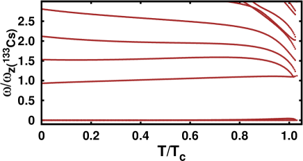
Figure 6: (Color online) Frequencies ($\displaystyle\omega_{j}$) of the low-lying modes at $\displaystyle T/T_{c}\neq 0$. The filled circles (brown) are the excitation energies from the HFB-Popov theory with $\displaystyle N_{\rm Rb}=N_{\rm Cs}=10^{3}$. The blue colored points indicate the location of the mode bifurcation.

III.3 Mode evolution of trapped TBEC at $\displaystyle T\neq 0$

For the $\displaystyle T\neq 0$ calculations, as mentioned earlier, we solve the coupled Eq. (3) and (4) iteratively till convergence. After each iteration, $\displaystyle\phi_{k}(z)$ are renormalized so that

$$\int_{-\infty}^{\infty}\left[|\phi_{k}(z)|^{2}+\tilde{n}_{k}(z)\right]dz=N_{k},$$ (9)

where $\displaystyle k$ is either Rb or Cs. To improve convergence, we use successive over relaxation, but at higher $\displaystyle T$ we face difficulties and require careful choice of the relaxation parameters. For computations, we again consider the trap parameters $\displaystyle\omega_{\perp({\rm Cs})}=2\pi\times 40.2$Hz and $\displaystyle\omega_{\perp({\rm Rb})}=2\pi\times 32.2$Hz with coinciding trap centers, the number of atoms as $\displaystyle N_{\rm Rb}=N_{\rm Cs}=10^{3}$ and $\displaystyle a_{\rm CsRb}=650a_{0}$. The evolution of $\displaystyle\omega$ (mode frequency) with $\displaystyle T$ is shown in Fig. 6, where the $\displaystyle T$ is in units of $\displaystyle T_{c}$, the critical temperature of ideal bosons in quasi-1D harmonic traps defined through the relation $\displaystyle N=(k_{\rm B}T_{c}/\hbar\omega_{z})\ln(2k_{\rm B}T_{c}/\hbar\omega_{z})$ Ketterle and van Druten (1996), where $\displaystyle N$ is the number of atoms. Considering that $\displaystyle\omega_{z({\rm Rb})}<\omega_{z({\rm Cs})}$, the critical temperature of Rb is lower than that of Cs. So, for better description we scale the temperature with respect to the $\displaystyle T_{c}$ of Rb atoms, and here after by $\displaystyle T_{c}$ we mean the critical temperature of Rb atoms. From the figure, when $\displaystyle T/T_{c}\geqslant 0.2$ the Kohn mode energy increases with $\displaystyle T/T_{c}$. This is consistent with an earlier work on HFB-Popov studies in single species condensate Gies et al. (2004), but different from the trend observed in ref. Hutchinson et al. (1997); Dodd et al. (1998). The increase in Kohn mode energy could arise from an important factor associated with the thermal atoms. In the HFB-Popov formalism the collective modes oscillates in a static thermal cloud background and dynamics of $\displaystyle\tilde{n}_{k}$ is not taken into account. In TBECs the effects of dynamics of $\displaystyle\tilde{n}_{k}$ may be larger as $\displaystyle\tilde{n}_{k}$ is large at the interface. An inclusion of the full dynamics of the thermal cloud in the theory would ensure the Kohn mode energy to be constant at all temperatures Hutchinson et al. (2000). The Goldstone modes, on the other hand, remain steadyGies et al. (2004).

The trend in the evolution of the modes indicates bifurcations at $\displaystyle T/T_{c}\approx 1$ and is consistent with the theoretical observations in single species condensates Hutchinson et al. (1997); Dodd et al. (1998); Gies et al. (2004). At this temperature, as evident from Fig. 6, the Kohn mode and the mode above it (which has principal quantum no $\displaystyle n=2$ for both the species ) merges. For brevity, the location of the mode bifurcation is indicated by the blue colored points in Fig. 6. This is one of the bifurcations emerging from the Rb atoms crossing the critical temperature, above this temperature there are no Rb condensates atoms. At $\displaystyle T>T_{c}$ the Cs condensate density is still non-zero as Cs has higher critical temperature. So, there may be another mode-bifurcation at the critical temperature of Cs. A reliable calculation for this would, however, require treating the interaction between thermal Rb atoms and Cs condensate more precisely. For this reason in the present work we do not explore temperature much higher than the $\displaystyle T_{c}$ of Rb atoms and the possibility of the second mode bifurcation shall be examined in our future works. In the case of single species calculations, at $\displaystyle T/T_{c}>1$ the mode frequencies coalesce to the mode frequencies of the trapping potential. In the present work we limit the calculations to $\displaystyle 0\leqslant T/T_{c}\leqslant 1.1$, so that $\displaystyle T/T_{c}\ll T_{d}/T_{c}$. Here, $\displaystyle T_{d}\approx(N_{\rm Rb}+N_{\rm Cs})\hbar\omega_{z}/k_{\rm B}$ is the degeneracy temperature of the system and in the present case $\displaystyle T_{d}\approx 437$nK. The results for $\displaystyle T/T_{c}>0.65$ may have significant errors as the HFB-Popov theory gives accurate results at $\displaystyle T/T_{c}\leqslant 0.65$ Dodd et al. (1998). We have, however, extended the calculations to $\displaystyle T/T_{c}>0.65$ like in Ref. Hutchinson et al. (1997) to study the mode bifurcation.

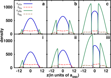
Figure 7: (Color online) Density profile of $\displaystyle n_{c}$ and $\displaystyle\tilde{n}$ at 25nK. (a), (b) and (c) correspond to $\displaystyle N_{\rm Rb}=840(N_{\rm Cs}=8570)$, $\displaystyle N_{\rm Rb}=3680(N_{\rm Cs}=8510)$, and $\displaystyle N_{\rm Rb}=15100(N_{\rm Cs}=6470)$, respectively, with coincident trap centers. (i), (ii) and (iii) correspond to same atom numbers as the previous sequence, however, the trap centers are shifted relatively by 0.8$\displaystyle a_{\rm osc(Cs)}$. In the plots density is measured in units of $\displaystyle a_{\rm osc}^{-1}$.

To examine the profiles of $\displaystyle n_{ck}$ and $\displaystyle\tilde{n}_{k}$, we compute the densities at 25nK for three cases, these are $\displaystyle N_{\rm Rb}=840(N_{\rm Cs}=8570)$, $\displaystyle N_{\rm Rb}=3680(N_{\rm Cs}=8510)$, and $\displaystyle N_{\rm Rb}=15100(N_{\rm Cs}=6470)$. The same set was used in the previous work of Pattinson, et al. at $\displaystyle T=0$ Pattinson et al. (2013) and correspond to three regimes considered ($\displaystyle N_{\rm Cs}>N_{\rm Rb}$, $\displaystyle N_{\rm Cs}\approx N_{\rm Rb}$, and $\displaystyle N_{\rm Cs}<N_{\rm Rb}$) in the experimental work of McCarron, et al. McCarron et al. (2011). Consider the trap centers, along $\displaystyle z$-axis, are coincident, then $\displaystyle\tilde{n}_{k}$ and $\displaystyle n_{ck}$ are symmetric about $\displaystyle z=0$, and are shown in Fig. 7(a-c). In all the cases, $\displaystyle n_{\rm Cs}$ is at the center. This configuration is energetically preferred as heavier atomic species at the center has smaller trapping potential energy and lowers the total energy. In the experiments, the trap centers are not exactly coincident. So, to replicate the experimental situation we shift the trap centers, along $\displaystyle z$-axis, by 0.8$\displaystyle a_{\rm osc(Cs)}$ and $\displaystyle n$ are shown in Fig. 7(i-iii). For $\displaystyle N_{\rm Rb}=840(N_{\rm Cs}=8570)$ and $\displaystyle N_{\rm Rb}=3680(N_{\rm Cs}=8510)$, Fig. 7(i-ii), the $\displaystyle n_{ck}$ and $\displaystyle\tilde{n}_{k}$ are located sideways. So, there are only two Goldstone modes in the excitation spectrum. But, for $\displaystyle N_{\rm Rb}=15100(N_{\rm Cs}=6470)$, Fig. 7 (iii), $\displaystyle n_{\rm Cs}$ is at the center with $\displaystyle n_{\rm Rb}$ at the edges forming sandwich geometry and hence has three Goldstone modes. In all the cases $\displaystyle\tilde{n}_{k}$ have maxima in the neighbourhood of the interface and the respective $\displaystyle n_{ck}$s are not negligible. So, we can expect larger $\displaystyle n_{ck}$-$\displaystyle\tilde{n}_{k}$ coupling in TBECs than single species condensates. For the $\displaystyle N_{\rm Rb}=3680(N_{\rm Cs}=8510)$ and $\displaystyle N_{\rm Rb}=15100(N_{\rm Cs}=6470)$ cases, $\displaystyle n_{ck}$ are very similar to the results of 3D calculations at $\displaystyle T=0$ Pattinson et al. (2013). However, it requires a 3D calculation to reproduce $\displaystyle n_{ck}$ for $\displaystyle N_{\rm Rb}=840(N_{\rm Cs}=8570)$ as the relative shift $\displaystyle\delta x$ is crucial in this case.

IV Conclusions

TBECs with strong inter-species repulsion with sandwich density profile at phase-separation are equivalent to three coupled condensate fragments. Because of this we observe three Goldstone modes in the system after phase-separation. At higher inter-species interactions, we predict avoided crossings involving three modes and followed with the coalescence or quasi-degeneracy of two of the participating modes. At $\displaystyle T\neq 0$ there are mode bifurcations close to the $\displaystyle T/T_{c}\approx 1$.