Alignment of the Angular Momentum Vectors of Planetary Nebulae in the Galactic Bulge

Abstract

We use high-resolution H $\alpha$ images of 130 planetary nebulae (PNe) to investigate whether there is a preferred orientation for PNe within the Galactic Bulge. The orientations of the full sample have an uniform distribution. However, at a significance level of 0.01, there is evidence for a non-uniform distribution for those planetary nebulae with evident bipolar morphology. If we assume that the bipolar PNe have an unimodal distribution of the polar axis in Galactic coordinates, the mean Galactic position angle is consistent with $90\degr$, i.e. along the Galactic plane, and the significance level is better than 0.001 (the equivalent of a $3.7\sigma$ significance level for a Gaussian distribution).

The shapes of PNe are related to angular momentum of the original star or stellar system, where the long axis of the nebula measures the angular momentum vector. In old, low-mass stars, the angular momentum is largely in binary orbital motion. Consequently, the alignment of bipolar nebulae that we have found indicates that the orbital planes of the binary systems are oriented perpendicular to the Galactic plane. We propose that strong magnetic fields aligned along the Galactic plane acted during the original star formation process to slow the contraction of the star forming cloud in the direction perpendicular to the plane. This would have produced a propensity for wider binaries with higher angular momentum with orbital axes parallel to the Galactic plane. Our findings provide the first indication of a strong, organized magnetic field along the Galactic plane that impacted on the angular momentum vectors of the resulting stellar population.

1 Introduction

Planetary nebulae (PNe) are the ionized ejecta from evolved stars. They form when a low to intermediate-mass star, ascending the Asymptotic Giant Branch, ejects its envelope in a phase of pulsational instability. The remaining stellar core evolves to high temperatures and ionizes the expanding ejecta, before its nuclear burning ceases and the star becomes a white dwarf (Herwig, 2005; van Winckel, 2003).

PNe show a variety of morphologies; they range from round to strongly elliptical, together with bipolar and (infrequently) irregular shapes (Corradi & Schwarz, 1995; Balick & Frank, 2002; Parker et al., 2006). The origin of those morphologies is disputed. The main contenders are binarity and magnetic fields (de Marco, 2009; Blackman, 2009). Magnetic fields have been detected in PNe (Sabin, Zijlstra & Greaves, 2007; Vlemmings & van Langevelde, 2008; Gómez et al., 2009) but may not be strong enough to affect the outflows. Soker (2006) has argued that magnetic fields also require binary companions for their origin. If so, ultimately, in either case, the morphology is related to angular momentum in the stellar system and the major axis of the nebula traces the direction of the angular momentum vector.

Weidmann & Díaz (2008) have reported that PNe in the direction of the Galactic centre may have a preferential orientation, in terms of an excess population at one particular orientation. An alignment between adjacent but unrelated PNe is unexpected. However, if the orientation of a PN traces the angular momentum vector of the progenitor system, such an effect could originate from the formation of the stellar population. But the orientations could also be influenced by some external factor, for instance the Galactic magnetic field. This has been argued to be important for supernova remnants (Gaensler, 1998).

Studies of the orientation of PNe have been carried out for over thirty years with conflicting results (Schwarz, Monteiro & Peterson, 2008). There has been no convincing evidence for an alignment among nearby Galactic PNe, although there have been some claims for a preferential alignment of the polar axis with the Galactic plane (Melnick & Harwit, 1975). The evidence of Weidmann & Díaz (2008) is based on a sample of 440 PNe that were either bipolar, or elliptical with a major to minor axis ratio greater than $1.2:1$ of which 262 were in the direction of the Galactic centre. Within that group they found an excess of PNe with galactic position angle (GPA) $\sim 100\degr\$.

In this paper we use a morphological survey of 130 PNe likely to be in the Galactic Bulge to test this claim. As only 19 objects are in common with Weidmann & Díaz (2008), this provides an independent test of the potential alignment. The whole of the area containing our sample of PNe lies within one of the four regions (the Galactic Centre) studied by Weidmann & Díaz (2008). A number of our objects would not be classified as elongated by those authors and the higher angular resolution of our sample enables us to use objects with a smaller angular size than is permitted in their sample.

2 The Observations

The initial sample of PNe images consisted of 161 objects observed in 2003 using the EMMI instrument of the European Southern Observatory (ESO) 3.5 m New Technology Telescope (NTT) and 37 objects observed in 2002 and 2003 using the Planetary Camera of the WFPC2 of the HST (programmes 71.D-0448(A) and 9356 respectively). After removing foreground objects as described below, the final Bulge sample used in this paper contained 96 NTT objects and 34 HST objects.

The HST targets were selected as a random subset of compact PNe in the direction of the Bulge. We selected all PNe listed in the Strasbourg-ESO catalog of Galactic planetary nebulae (Acker et al., 1992), with a listed diameter of 4 arcsec or less, or no known diameter. Every second object from this list was selected for an HST SNAPshot program. Of the 60 objects selected, just over half were observed. The observations utilized the F656N filter (2.2 nm wide at 656.4 nm). The exposure times were about 120 seconds. The images have a pixel size of 0.046 arcsec.

The NTT sample was selected from the larger nebulae in and towards the Galactic Bulge. The NTT observations utilized the #654 H $\alpha$ filter (3.3 nm wide at 655.4 nm). The images have a pixel size of 0.33 arcsec (Gonzalez, Brilliant & Pompei, 2006). The seeing was typically better than 1.5 arcsec and the exposure times were mostly 60 s but a few were of 30, 120, 180, 240 and 300 seconds.

In the region studied, 80 per cent of the selected objects are expected to belong to the Galactic Bulge (Zijlstra, 1990) leaving few foreground nebulae in the sample. However, we removed PNe from the sample if they were likely foreground (or background) objects, not related to the Bulge, on the basis of the following criteria:

1. The PN lies beyond 10° of the Galactic centre in terms of Galactic longitude and latitude.

2. The PN has a measured component of length of more than 35 arcsec; see Acker, Peyaud & Parker (2006).

3. Where a radio flux at 5 GHz was available for the PN, for that flux to lie outside the interval $\left(4.2\mathrm{~{}mJy},\>59.1\mathrm{~{}mJy}\right)$ (Siódmiak & Tylenda, 2001; Acker et al., 1992).

It should be noted that PNe remained in the sample unless there was data that could be used to exclude them. Where two catalogues gave conflicting radio fluxes the PN was retained in the sample if one of those sets of data permitted it.

The NTT images were deconvolved using the LUCY/WAVE algorithm in the ESO/MIDAS package before determining the PNe morphologies and orientations. The HST images did not require deconvolution.

We define three morphological categories: bipolar, polar, and non-polar. We had no irregular PNe for which we could fix an orientation. PNe with one or more lobes, or the remnants of lobes, generally at the 1 per cent intensity level were classified as having a bipolar morphology. The bipolar class conforms in the main to that usually used, see Corradi & Schwarz (1995). We also followed those authors in not using a separate round class and classifying what might be considered as round PNe as elliptical. Due to the high resolution of the images we were able to split the elliptical category into two distinct classes. A PN was categorized as having a polar morphology if its image showed no lobes but the intensity distribution above 10 per cent of the peak flux level showed internal structure thus assisting in the identification of the polar axis. The remaining PNe were classified as non-polar. Fig. 1 shows examples from each of the classes.

$\begin{array}[]{cc}\includegraphics[width=213.39566pt]{Figure1_TopLeft}&\includegraphics[width=213.39566pt]{Figure1_TopRight}\\ \includegraphics[width=213.39566pt]{Figure1_CentreLeft}&\includegraphics[width=213.39566pt]{Figure1_CentreRight}\\ \includegraphics[width=213.39566pt]{Figure1_BottomLeft}&\includegraphics[width=213.39566pt]{Figure1_BottomRight}\par\end{array}$

Figure 1: Examples of the classifications of the PNe. PN G 000.2-01.9 was classified as bipolar and PN G 002.7-04.8 was classified as multilobed bipolar. PN G 003.2-06.2 was also classified as bipolar, i.e point symmetry does not form a class of its own, as was PN G 359.8+05.2, a bipolar remnant, i.e. our bipolar category includes those PNe deemed to be the remnants of bilobed or multilobed PNe. PN G 352.6+03.0 was classified as polar as it has no lobes and the contours suggest less material in the north and south directions. PN G 001.7-05.7 shows no internal structure and was classified as non-polar. The greyscale has black as high flux density. The isophotes are shown in red and are based on 10 per cent intervals of the peak PN flux density. The tick marks on the images without a scale bar indicate separations of 5 arcsec and those images have north to the top and east to the left.

The PN orientation was taken to be that of the polar or major axis of the PN as measured from North to East in the image, and converted to Galactic coordinates. The angle was estimated by eye over the range $\left[0\degr\ ,180\degr\ \right)$ with the assistance of the ruler tool in the NASA HEASARC fv system. The polar angle of a bipolar PN was determined by the alignment of the lower intensity interior of its central shell and the direction of its lobes. The polar angle of a non-polar PN was taken to be that of the major axis at the 10% level, basically the main symmetry axis of the nebula as suggested in Corradi, Aznar & Mampaso (1998) and Weidmann & Díaz (2008). For the polar PN, the direction of a central cavity and/or low intensity regions suggesting the direction of mass loss was used to assist in the determination of the polar angle. We used the alignments in the high intensity structures to determine the polar angles of the bipolar remnants, except that for PN G 359.8+05.2 we took the alignment to be perpendicular to that of the high intensity structure. Isophote plots of the bipolar PNe, including the bipolar remnants, overlaid with lines indicating the PN orientation and the uncertainty in that orientation are provided online. Only PNe whose orientation could readily be determined were included in the sample. Note that projection effects were not taken into account, i.e. the angles were measured in the plane of the sky, as we have no information of structure along the line of sight. The orientations for the polar and non-polar PNe were taken to have random uncertainties of 2°. Initially we also used that value for the uncertainties in the orientations of the bipolar PNe. However, to ensure that the evidence of alignment that we obtained in the statistical tests for those PNe was not down to using uncertainties that were too small we repeated the tests on the bipolar PNe using more carefully measured uncertainties. For the bipolar PNe we used an uncertainty that is the maximum of:

1. the estimated population standard deviation of repeated measurements of the orientation of the PN;

2. the arctangent of the reciprocal of the PN’s tip-to-tip length in pixels (to allow for a minimum of 1 pixel variation to account for the image resolution); and

3. 2°.

Overall, 68 of the observed PNe were rejected due to the selection criteria, imaging problems or uncertain orientation. The data set that remained consisted of 130 PNe split into the subsamples described above.

It should be noted that 19 of the PNe, just under one sixth of our final sample, are also in the analysis presented in Weidmann & Díaz (2008). According to our criteria, 5 of those 19 are bipolar, 10 polar and 4 non-polar.

The formula presented in Corradi, Aznar & Mampaso (1998) and the galactic coordinates quoted in SIMBAD for each PN were used to convert the measured polar angles (PA) of the PNe to galactic position angles (GPA). Both sets of values are shown in Table 1 and plots of the orientations of the PNe in the sample and main subsamples are shown in Fig. 2.

Table 1: The orientations of the PNe. The measurement of the position angles and the derivation of their uncertainties and of the GPA are described in Section 2. The uncertainties in the PA and GPA are identical.

PNG	Morphology	PA/°	GPA/°		Telescope	PNG	Morphology	PA/°	GPA/°		Telescope
000.1+02.6	polar	78	135$\pm$	2	NTT	007.8 – 03.7	polar	171	53$\pm$	2	NTT
000.1+04.3	non-polar	105	162$\pm$	2	NTT	007.8 – 04.4	non-polar	111	173$\pm$	2	NTT
000.1 – 02.3	polar	70	129$\pm$	2	NTT	008.2+06.8	bipolar	68	127$\pm$	2	HST
000.2 – 01.9	bipolar	105	165$\pm$	4	NTT	008.4 – 03.6	bipolar	149	31$\pm$	2	NTT
000.3 – 04.6	bipolar	71	132$\pm$	2	NTT	008.6 – 02.6	non-polar	162	44$\pm$	2	HST
000.4 – 01.9	bipolar	35	95$\pm$	5	NTT	009.4 – 09.8	polar	86	150$\pm$	2	NTT
000.4 – 02.9	polar	174	54$\pm$	2	NTT	009.8 – 04.6	bipolar	33	95$\pm$	9	NTT
000.7+03.2	bipolar	179	57$\pm$	2	NTT	350.5 – 05.0	polar	48	107$\pm$	2	NTT
000.7 – 02.7	non-polar	133	13$\pm$	2	NTT	351.1+04.8	polar	159	32$\pm$	2	HST
000.7 – 03.7	polar	75	136$\pm$	2	NTT	351.2+05.2	bipolar	120	172$\pm$	5	NTT
000.7 – 07.4	bipolar	152	35$\pm$	4	NTT	351.6 – 06.2	polar	121	0$\pm$	2	NTT
000.9 – 02.0	non-polar	19	79$\pm$	2	NTT	351.9+09.0	bipolar	54	105$\pm$	6	NTT
000.9 – 04.8	polar	141	22$\pm$	2	NTT	351.9 – 01.9	bipolar	15	72$\pm$	2	HST
001.2+02.1	polar	12	70$\pm$	2	HST	352.0 – 04.6	non-polar	155	34$\pm$	2	NTT
001.2 – 03.0	non-polar	155	35$\pm$	2	NTT	352.1+05.1	polar	131	5$\pm$	2	NTT
001.3 – 01.2	polar	56	116$\pm$	2	NTT	352.6+03.0	polar	178	53$\pm$	2	HST
001.4+05.3	bipolar	42	99$\pm$	3	NTT	353.2 – 05.2	bipolar	46	105$\pm$	6	NTT
001.7+05.7	non-polar	116	173$\pm$	2	NTT	353.3+06.3	non-polar	33	86$\pm$	2	NTT
001.7 – 04.4	polar	84	145$\pm$	2	HST	353.7+06.3	polar	0	53$\pm$	2	NTT
002.0 – 06.2	non-polar	145	27$\pm$	2	NTT	354.5+03.3	bipolar	102	157$\pm$	2	HST
002.1 – 02.2	non-polar	117	177$\pm$	2	NTT	354.9+03.5	polar	99	154$\pm$	2	HST
002.1 – 04.2	non-polar	167	48$\pm$	2	NTT	355.1 – 06.9	bipolar	25	86$\pm$	8	NTT
002.2 – 09.4	bipolar	149	33$\pm$	4	NTT	355.4 – 02.4	bipolar	154	32$\pm$	2	HST
002.3+02.2	polar	143	21$\pm$	2	NTT	355.6 – 02.7	non-polar	90	149$\pm$	2	NTT
002.3 – 03.4	polar	163	44$\pm$	2	HST	355.9+03.6	non-polar	77	133$\pm$	2	HST
002.5 – 01.7	polar	90	150$\pm$	2	NTT	355.9 – 04.2	polar	106	165$\pm$	2	NTT
002.6+02.1	bipolar	68	127$\pm$	5	NTT	356.3 – 06.2	polar	67	128$\pm$	2	NTT
002.7 – 04.8	bipolar	33	95$\pm$	4	NTT	356.5 – 03.6	bipolar	57	117$\pm$	3	HST
002.8+01.7	polar	9	68$\pm$	2	HST	356.8+03.3	bipolar	28	84$\pm$	8	HST
002.8+01.8	polar	43	102$\pm$	2	NTT	356.8 – 05.4	polar	175	56$\pm$	2	NTT
002.9 – 03.9	polar	15	76$\pm$	2	HST	356.9+04.4	bipolar	45	100$\pm$	6	HST
003.1+03.4	polar	157	35$\pm$	2	HST	357.0+02.4	polar	139	16$\pm$	2	NTT
003.2 – 06.2	bipolar	144	26$\pm$	6	NTT	357.1+03.6	polar	40	96$\pm$	2	NTT
003.6+03.1	bipolar	26	85$\pm$	2	HST	357.1+04.4	polar	70	126$\pm$	2	NTT
003.6 – 02.3	bipolar	136	17$\pm$	5	NTT	357.1 – 04.7	bipolar	164	44$\pm$	3	HST
003.7+07.9	polar	0	57$\pm$	2	NTT	357.2+02.0	non-polar	90	147$\pm$	2	HST
003.8 – 04.3	polar	23	85$\pm$	2	NTT	357.3+04.0	non-polar	68	124$\pm$	2	NTT
003.9+01.6	polar	59	118$\pm$	2	NTT	357.5+03.1	non-polar	72	128$\pm$	2	NTT
003.9 – 02.3	polar	138	19$\pm$	2	NTT	357.5+03.2	bipolar	26	83$\pm$	5	NTT
003.9 – 03.1	polar	105	166$\pm$	2	HST	357.6 – 03.3	bipolar	32	91$\pm$	7	NTT
004.0 – 03.0	polar	81	142$\pm$	2	HST	357.9 – 03.8	polar	65	125$\pm$	2	NTT
004.1 – 03.8	non-polar	6	67$\pm$	2	HST	357.9 – 05.1	bipolar	35	96$\pm$	5	NTT
004.2 – 03.2	non-polar	51	112$\pm$	2	NTT	358.0+09.3	non-polar	16	70$\pm$	2	NTT
004.2 – 04.3	non-polar	114	176$\pm$	2	NTT	358.2+03.5	non-polar	69	125$\pm$	2	NTT
004.2 – 05.9	bipolar	39	102$\pm$	7	NTT	358.2+04.2	non-polar	150	26$\pm$	2	NTT
004.3+01.8	bipolar	37	96$\pm$	2	NTT	358.5+02.9	polar	30	87$\pm$	2	HST
004.6+06.0	non-polar	71	129$\pm$	2	NTT	358.5 – 04.2	bipolar	157	37$\pm$	4	HST
004.8+02.0	non-polar	35	95$\pm$	2	HST	358.6+07.8	non-polar	127	2$\pm$	2	NTT
004.8 – 05.0	polar	0	62$\pm$	2	NTT	358.6 – 05.5	bipolar	18	79$\pm$	5	NTT
005.0 – 03.9	polar	165	47$\pm$	2	NTT	358.7+05.2	polar	82	138$\pm$	2	HST
005.2+05.6	polar	166	44$\pm$	2	NTT	358.8+03.0	polar	90	147$\pm$	2	NTT
005.5+06.1	bipolar	31	88$\pm$	2	NTT	358.9+03.4	bipolar	73	129$\pm$	2	HST
005.5 – 04.0	polar	134	16$\pm$	2	NTT	359.0 – 04.1	polar	40	100$\pm$	2	NTT
005.8 – 06.1	polar	63	126$\pm$	2	NTT	359.1 – 02.9	bipolar	63	123$\pm$	4	NTT
005.9 – 02.6	bipolar	62	123$\pm$	3	NTT	359.2+04.7	polar	164	40$\pm$	2	HST
006.1+08.3	polar	90	147$\pm$	2	HST	359.3 – 01.8	bipolar	54	113$\pm$	5	NTT
006.3+03.3	non-polar	32	91$\pm$	2	NTT	359.6 – 04.8	polar	68	129$\pm$	2	NTT
006.3+04.4	polar	116	175$\pm$	2	HST	359.7 – 01.8	polar	129	8$\pm$	2	NTT
006.4+02.0	bipolar	4	63$\pm$	2	HST	359.8+02.4	non-polar	9	66$\pm$	2	NTT
006.8+02.3	polar	148	28$\pm$	2	NTT	359.8+03.7	bipolar	27	84$\pm$	4	NTT
006.8 – 03.4	non-polar	171	53$\pm$	2	NTT	359.8+05.2	bipolar	68	125$\pm$	5	NTT
007.0 – 06.8	bipolar	20	80$\pm$	10	NTT	359.8+05.6	bipolar	68	124$\pm$	5	NTT
007.5+04.3	non-polar	119	178$\pm$	2	HST	359.8+06.9	bipolar	156	31$\pm$	4	NTT
007.5+07.4	polar	90	148$\pm$	2	NTT	359.8 – 07.2	non-polar	124	6$\pm$	2	NTT
007.6+06.9	polar	54	112$\pm$	2	NTT	359.9 – 04.5	polar	137	18$\pm$	2	NTT

$\begin{array}[]{cc}\includegraphics[width=221.93158pt]{Figure2_TopLeft}&\includegraphics[width=221.93158pt]{Figure2_TopRight}\\ \includegraphics[width=221.93158pt]{Figure2_CentreLeft}&\includegraphics[width=221.93158pt]{Figure2_CentreRight}\\ \includegraphics[width=221.93158pt]{Figure2_BottomLeft}&\includegraphics[height=221.93158pt]{Figure2_BottomRight}\end{array}$

Figure 2: The GPA of the PNe in the samples. They are plotted on a background of contour plots of the 21 cm radio continuum polarization angles in the Galactic Bulge which are based on data (Testori, Reich & Reich, 2008) obtained from Max-Planck-Institut für Radioastronomie Survey Sampler (available from: http://www.mpifr-bonn.mpg.de/survey.html). The polarization angles are with respect to the Galactic North Pole and their magnitudes are indicated by the scale bar at the bottom right. We discuss the use of that polarization data in §4.

3 The Analysis

The analysis was performed using Matlab^®, Mathematica^® and CircStat, the circular statistics toolbox for Matlab, (Berens, 2009). The full sample and the subsamples of bipolar, elliptical, polar and non-polar PNe were analysed as were subsamples of them based on a split north and south, and east and west of the Galactic Centre.

The orientation angles occupied almost the whole semicircular range so an angle of 1°  modulo 180°  is closer to an angle of 175°  than it is to one of 10°. Consequently the circular nature of the data could not be ignored. Circular statistics techniques were used to investigate its distribution and the statistical tests needed to be invariant under a rotation of the axes.

As the orientations are axial rather than vector, the angles range only over 180 degrees. These were doubled to bring them to modulo 360° for much of the analysis, see Fisher (1995).

As an initial step, finger plots of the distribution of the GPA and rose plots (a circular form of bar chart) of the doubled angles were produced for all the samples. The finger plots provide the fine detail of the information and avoid the possibly misleading effects of grouping that can occur with any type of histogram. The plots for the overall sample and the main subsamples are presented in Figs. 3 and 4.

$\begin{array}[]{cc}\includegraphics{Figure3_TopLeft}&\includegraphics{Figure3_TopRight}\\ \includegraphics{Figure3_CentreLeft}&\includegraphics{Figure3_CentreRight}\\ \includegraphics{Figure3_BottomLeft}&\includegraphics{Figure3_BottomRight}\end{array}$

Figure 3: Finger plots of the GPA and the rose plots of the doubled GPA for the whole sample, the bipolar PNe and the elliptical (polar and non-polar) PNe over the whole area. Each dot on a finger plot represents a GPA in the subsample. The radial scale on the rose plots indicates the number of objects.

$\begin{array}[]{cc}\includegraphics{Figure4_TopLeft}&\includegraphics{Figure4_TopRight}\\ \includegraphics{Figure4_BottomLeft}&\includegraphics{Figure4_BottomRight}\end{array}$

Figure 4: Finger plots of the GPA and the rose plots of the doubled angles for the polar and non-polar PNe over the whole area. Each dot on a finger plot represents a GPA in the subsample. The radial scale on the rose plots indicates the number of objects.

Quantile–quantile (Q–Q) plots (a type of probability-probability plot) of the data for each sample were also prepared (Fisher, 1995) and those for the whole sample and the morphological subsamples are shown in Fig. 5. The plots are extended below (0,0) and above (1,1) with mirrored data from the other end of the plot. This extension is designed to avoid any misleading effect due to the linear representation of circular data. Points from an uniform distribution would lie on a 45°  line from the bottom left to top right of such a plot. Departures from that angle indicate departures from uniformity.

The mean GPA values were derived in the usual way for axial data i.e. as a vector summation over 360°  then halved.

$\begin{array}[]{cc}\includegraphics[width=230.46748pt]{Figure5_TopLeft}&\includegraphics[width=230.46748pt]{Figure5_TopRight}\\ \includegraphics[width=230.46748pt]{Figure5_CentreLeft}&\includegraphics[width=230.46748pt]{Figure5_CentreRight}\\ \includegraphics[width=230.46748pt]{Figure5_BottomLeft}&\end{array}$

Figure 5: The extended quantile-quantile (Q–Q) plots for the full sample and the principal subsamples over the whole area. Q-Q plots for the bipolar PNe in the North, South, East and West subsamples are available online.

A Rayleigh test, a Hodges-Ajne test, a Kuiper test and a Watson U² test for a null hypothesis of uniformity against an alternative hypothesis of non-uniformity were made. The Kuiper test has the advantage that it tests for randomness against any other alternative whereas the Rayleigh test assumes an unimodal alternative (Fisher, 1995). However, if the alternative is a von Mises distribution (also known as the Circular Normal Distribution), the Rayleigh test is the most powerful invariant test for uniformity (Bogdan, Bogdan & Futschik, 2002). The Hodges-Ajne test counts numbers on arbitrary semi-circles and checks for an excess on one side of the circle. It can also be used for samples from any distribution (Jammalamadaka & SenGupta, 2001; Hoenen & Gnaspini, 1999; Protheroe, 1985) and is useful when a peak in the number of events is likely to be confined to one half of the angular range. Rayleigh tests for the same null hypothesis against alternative hypotheses of an unimodal distribution with mean angles of 90° (i.e. along the Galactic Plane) and 100° , the angle of the excess found by Weidmann & Díaz (2008), were also performed. The p–values for the Kuiper and Watson U² tests were obtained using Mathematica’s ‘DistributionFitTest’. We initially used CircStat (Berens, 2009) to obtain the p–values for the Hodges-Ajne test but we then modified the procedure to work in Mathematica as using one statistical package for all the statistical tests for uniformity simplified bootstrapping. The Rayleigh tests used the formulae presented in Fisher (1995). The tests are right tail (one-sided excess) tests, where small p–values would lead us to reject $\mathrm{H}_{0}$.

In order to check the effect of the uncertainties in the orientations, the full area tests were repeated after adding randomly selected values from a $\mathrm{N}\left(0,\sigma^{2}\right)$ distribution, where $\sigma$ is the uncertainty. This process was repeated 100 000 times. We also used bootstrapping to produce a sampling distribution of the p-values. We repeated this with each of the bootstrapped angles adjusted by a value from its $\mathrm{N}\left(0,\sigma^{2}\right)$ distribution (a smoothed bootstrap).

4 Results

It can already be seen from the rose plots in Figs. 3 and 4 that the plot for the bipolar PNe is less balanced than those for the other classifications.

Some indications of the uniformity of the distributions of the GPA can be seen from the Q–Q plots in Fig. 5. The deviations from the 45°  line tend to increase as the sample size decreases, a situation that can also be seen in the plots for the area subsamples. However, the bipolar sample and its area subsamples have greater deviations than do the elliptical sample and its area subsamples. Note the pronounced deviation from a 45° slope at approximately (0.5,0.5) in the plot for the bipolar data sample.

The p–values obtained for the single sample tests are listed in Table 2 as are the sample sizes. In all five tests the null hypothesis, H₀, is that the distribution of the GPA is uniform (i.e. when the angles are doubled to cover the full circle it is isotropic). The alternative hypothesis, H₁, for the four tests for uniformity is simply that the distribution is not uniform. H₁ for the Rayleigh tests against the mean are those of an unimodal distribution with a mean angle of 90° (i.e. along the Galactic Plane) or of 100° (i.e the angle of the excess found by Weidmann & Díaz (2008)).

Table 2: The data for the PNe samples and area sub-samples together with the p–values for the single sample tests. The angles are shown rounded to the nearest $1\degr$ and the p–values have been quoted to the first significant digit. The p–values derived for the non-polar south-west subsample have been excluded as the sample size of 3 indicates that they are not meaningful. The null hypothesis (H₀) for all the tests is that the distribution of the GPA is uniform. East (E), west (W), north (N) and south (S) are with respect to Galactic coordinates on either side of 0°longitude and latitude.

				p–values
Class	Area	sample	mean	Tests for Uniformity								Rayleigh Test
		size	GPA	H1: the distribution is not uniform								H1: an unimodal mean GPA of:
			/ ∘	Rayleigh		Hodges-Ajne		Kuiper		Watson U2		90∘		100∘
All	All	130	95	0.	3	0.	4	0.	3	0.	2	0.	06	0.	06
Bipolar	All	44	93	0.	0008	0.	02	0.	0002	0.	006	0.	00009	0.	0001
Elliptical	All	86	176	0.	8	0.	9	0.	5	0.	7	0.	2	0.	3
Polar	All	55	158	0.	9	0.	9	0.	6	0.	7	0.	4	0.	4
Non-polar	All	31	8	0.	7	0.	9	0.	9	0.	9	0.	2	0.	2
All	E	72	70	0.	6	0.	5	0.	8	0.	8	0.	2	0.	3
All	W	58	109	0.	2	0.	4	0.	1	0.	1	0.	06	0.	03
All	N	61	107	0.	1	0.	3	0.	1	0.	1	0.	04	0.	02
All	S	69	63	0.	7	0.	9	0.	8	0.	7	0.	3	0.	4
All	NE	28	99	0.	3	0.	8	0.	6	0.	5	0.	07	0.	06
All	NW	33	114	0.	3	0.	5	0.	3	0.	3	0.	2	0.	08
All	SE	44	40	0.	5	0.	6	0.	5	0.	6	0.	4	0.	3
All	SW	25	100	0.	5	0.	9	0.	4	0.	5	0.	1	0.	1
Bipolar	E	21	88	0.	08	0.	2	0.	1	0.	05	0.	01	0.	02
Bipolar	W	23	97	0.	008	0.	1	0.	005	0.	01	0.	001	0.	001
Bipolar	N	19	101	0.	006	0.	05	0.	002	0.	009	0.	001	0.	0006
Bipolar	S	25	84	0.	05	0.	1	0.	04	0.	02	0.	009	0.	02
Bipolar	NE	8	92	0.	02	0.	06	0.	02	0.	02	0.	002	0.	003
Bipolar	NW	11	111	0.	1	0.	1	0.	08	0.	1	0.	07	0.	03
Bipolar	SE	13	75	0.	7	0.	5	0.	6	0.	4	0.	2	0.	3
Bipolar	SW	12	87	0.	02	0.	06	0.	03	0.	03	0.	003	0.	007
Elliptical	E	51	24	0.	7	0.	9	0.	9	0.	8	0.	3	0.	2
Elliptical	W	35	148	0.	6	0.	5	0.	4	0.	5	0.	3	0.	5
Elliptical	N	42	129	0.	8	0.	9	0.	8	0.	9	0.	4	0.	4
Elliptical	S	44	11	0.	5	0.	8	0.	5	0.	5	0.	1	0.	1
Elliptical	NE	20	136	0.	9	0.	9	1.		1.		0.	5	0.	4
Elliptical	NW	22	124	0.	9	0.	9	0.	6	0.	8	0.	4	0.	4
Elliptical	SE	31	29	0.	4	0.	7	0.	7	0.	4	0.	2	0.	1
Elliptical	SW	13	159	0.	4	0.	5	0.	6	0.	5	0.	2	0.	3
Polar	E	33	21	1.		1.		0.	6	0.	7	0.	5	0.	5
Polar	W	22	155	0.	8	0.	9	0.	8	0.	9	0.	3	0.	4
Polar	N	26	41	0.	9	0.	9	0.	9	0.	9	0.	5	0.	4
Polar	S	29	147	0.	7	0.	7	0.	6	0.	6	0.	4	0.	5
Polar	NE	14	62	0.	9	0.	7	0.	9	1.		0.	4	0.	5
Polar	NW	12	22	0.	9	1.		0.	9	1.		0.	4	0.	3
Polar	SE	19	160	1.		1.		0.	7	0.	7	0.	4	0.	4
Polar	SW	10	143	0.	5	0.	5	0.	5	0.	5	0.	4	0.	5
Non-polar	E	18	24	0.	4	0.	5	0.	5	0.	4	0.	2	0.	1
Non-polar	W	13	140	0.	7	0.	9	0.	5	0.	7	0.	4	0.	4
Non-polar	N	16	129	0.	3	0.	8	0.	4	0.	3	0.	4	0.	2
Non-polar	S	15	27	0.	05	0.	07	0.	08	0.	08	0.	08	0.	02
Non-polar	NE	6	143	0.	5	0.	2	0.	3	0.	4	0.	4	0.	5
Non-polar	NW	10	119	0.	5	0.	5	0.	4	0.	4	0.	3	0.	2
Non-polar	SE	12	34	0.	08	0.	06	0.	1	0.	1	0.	2	0.	07
Non-polar	SW	3	4

The results for the bipolar PNe are shown in Table 3. Bootstrapping increases the mean p–value but reduces the median value. Estimates of the median p-values for the GPA for the whole area samples of the three morphologies and the two combined samples are presented in Table 4. They were obtained from derived from the bootstrapped plus $\mathrm{N}\left(0,\sigma^{2}\right)$ uncertainty runs. It can be seen that the results for the bipolar PNe can be considered as significant at, at worst, the 0.005 significance level.

Table 3: Sampling distributions of the p–values for the GPA of the bipolar PNe sample. There were 100 000 such samples for each of: the measured value plus a randomly selected $\mathrm{N}\left(0,\sigma^{2}\right)$ value where $\sigma$ is the uncertainty in the PN orientation, a bootstrapped selection from the measured values with duplicates adjusted by adding multiples of $10^{-8}$ degrees and the bootstrapped selection plus the randomly selected $\mathrm{N}\left(0,\sigma^{2}\right)$ value. Quoted uncertainties in the statistics are based on the distribution of 100 subsamples of size 1 000 where that distribution is judged to be Normal using an Anderson–Darling test at a 0.5 significance level.

test	method	mean		standard		quantiles
				deviation		median		16%		84%
Rayleigh	measured + $\mathrm{N}\left(0,\sigma^{2}\right)$	0.	00123$\pm$0.00002	0.	00065$\pm$0.00002	0.	00109$\pm$0.00002	0.	00066$\pm$0.00001	0.	00178$\pm$0.00004
	bootstrapped	0.	013$\pm$0.002	0.	046$\pm$0.007	0.	00050$\pm$0.00008	0.	000007$\pm$0.000002	0.	012$\pm$0.002
	bootstrapped + $\mathrm{N}\left(0,\sigma^{2}\right)$	0.	015$\pm$0.002	0.	051$\pm$0.007	0.	0006	0.	00001	0.	015$\pm$0.002
Hodges-Ajne	measured + $\mathrm{N}\left(0,\sigma^{2}\right)$	0.	02	0.	0137$\pm$0.0003	0.	02	0.	007	0.	05
	bootstrapped	0.	025$\pm$0.002	0.	058$\pm$0.006	0.	007	0.	0001	0.	05
	bootstrapped + $\mathrm{N}\left(0,\sigma^{2}\right)$	0.	025$\pm$0.002	0.	062$\pm$0.007	0.	002	0.	0001	0.	05
Kuiper	measured + $\mathrm{N}\left(0,\sigma^{2}\right)$	0.	00089$\pm$0.00003	0.	00095$\pm$0.00007	0.	00059$\pm$0.00002	0.	00022$\pm$0.00001	0.	00149$\pm$0.00006
	bootstrapped	0.	0017$\pm$0.0003	0.	009$\pm$0.003	0.	00003	0.	0000002	0.	0009
	bootstrapped + $\mathrm{N}\left(0,\sigma^{2}\right)$	0.	0026$\pm$0.0005	0.	01	0.	00007	0.	0000009$\pm$0.0000002	0.	002
Watson U2	measured + $\mathrm{N}\left(0,\sigma^{2}\right)$	0.	00650$\pm$0.00003	0.	00076$\pm$00002	0.	00651$\pm$0.00003	0.	00573$\pm$0.00003	0.	00725$\pm$0.00004
	bootstrapped	0.	0066$\pm$0.0005	0.	015$\pm$0.003	0.	0045$\pm$0.0002	0.	0000006	0.	0086$\pm$0.0001
	bootstrapped + $\mathrm{N}\left(0,\sigma^{2}\right)$	0.	0082$\pm$0.0007	0.	020$\pm$0.004	0.	0051$\pm$0.0002	0.	00002	0.	009$\pm$0.0002
Rayleigh	measured + $\mathrm{N}\left(0,\sigma^{2}\right)$	0.	000134$\pm$0.000002	0.	000080$\pm$0.000003	0.	000120$\pm$0.000003	0.	000069$\pm$0.000002	0.	000204$\pm$0.000005
H1: $90^{\circ}$	bootstrapped	0.	0032$\pm$0.0005	0.	015$\pm$0.003	0.	00008$\pm$0.00001	0.	0000012$\pm$0.0000003	0.	0024$\pm$0.0004
unimodal	bootstrapped + $\mathrm{N}\left(0,\sigma^{2}\right)$	0.	0039$\pm$0.0006	0.	017$\pm$0.004	0.	0001	0.	000002	0.	0031$\pm$0.0005
Rayleigh	measured + $\mathrm{N}\left(0,\sigma^{2}\right)$	0.	000200$\pm$0.000004	0.	000110$\pm$0.000005	0.	000175$\pm$0.000003	0.	000105$\pm$0.000002	0.	000290$\pm$0.000007
H1: $100^{\circ}$	bootstrapped	0.	0054$\pm$0.0007	0.	023$\pm$0.004	0.	00012$\pm$0.00002	0.	000001	0.	004
unimodal	bootstrapped + $\mathrm{N}\left(0,\sigma^{2}\right)$	0.	0062$\pm$0.0008	0.	025$\pm$0.004	0.	00016$\pm$0.00003	0.	000002	0.	0050$\pm$0.0008

Table 4: The median p–values for the GPA of the five single sample tests. The values and their uncertainties were obtained by bootstrapping the GPA and adding a randomly selected $\mathrm{N}\left(0,\sigma^{2}\right)$ value, where $\sigma$ is the uncertainty in the PN orientation for the bipolar PNe and 2°  for the other PNe. The median has been used due to the distributions of the p–values being skewed. There were 100 000 bootstraps. The samples of 100 000 were each split into subsamples of 1 000 and the mean and standard deviation of the median p-value obtained. Where the distribution of the medians was judged to be Normal using an Anderson–Darling test at a 0.5 significance level its standard deviation was used as the uncertainty, otherwise the p–value has been quoted to the first significant digit. The mean GPA quoted is that of the original sample.

			median p–values
Class	sample	mean	Tests for Uniformity								Rayleigh Test with H1:
	size	GPA	Rayleigh		Hodges-Ajne		Kuiper		Watson U2		an unimodal mean GPA of:
		/ ∘									90∘		100∘
All	130	95	0.	17$\pm$0.01	0.	1	0.	038$\pm$0.003	0.	082$\pm$0.005	0.	063$\pm$0.005	0.	061$\pm$0.005
Bipolar	44	93	0.	0006	0.	002	0.	00007	0.	0051$\pm$0.0002	0.	0001	0.	00016$\pm$0.00003
Elliptical	86	176	0.	40$\pm$0.02	0.	3	0.	16$\pm$0.01	0.	22$\pm$0.01	0.	205$\pm$0.009	0.	214$\pm$0.009
Polar	55	158	0.	47$\pm$0.01	0.	4	0.	152$\pm$0.008	0.	194$\pm$0.008	0.	264$\pm$0.008	0.	264$\pm$0.008
Non-polar	31	8	0.	39$\pm$0.02	0.	5	0.	24$\pm$0.01	0.	29$\pm$0.01	0.	186$\pm$0.008	0.	183$\pm$0.008

Runs were also performed for the GPA of the bipolar sample with the uncertainties increased by 5, 10 and 20 degrees in order to check the effects of larger uncertainties. As expected, increasing the uncertainties increases the probability that the GPA for the sample come from a randomly orientated population of bipolar Bulge PNe. The results are presented in Table 5. The median p–values for uncertainties increased by no more than 10° are all below 0.01 with those for the tests against the specified mean orientations below 0.001. With added 20° uncertainties the Rayleigh tests against the alternative hypotheses of unimodal distributions with mean values of 90° and 100° respectively, still produce p–values $\leq 0.01$. Any increase in the uncertainties above those estimated from the measurements would need to be large in order to change our conclusions.

Table 5: The effect of uncertainties in the orientations on the sampling distributions of the p–values for the GPA of the bipolar PNe sample. The results indicated to have 0°  additional uncertainty are those shown in the third row for each test in Table 3. They are for 100 000 bootstrapped selections from the measured values to which were added values randomly selected from a $\mathrm{N}\left(0,\sigma^{2}\right)$ distribution, where $\sigma$ is the uncertainty in the PN orientation. Those results are compared to three further sets of 100 000 for which $\sigma$ was increased by values of 5, 10 and 20°  respectively. Quoted uncertainties in the statistics are based on the distribution of 100 subsamples of size 1 000 where that distribution is judged to be Normal using an Anderson–Darling test at a 0.5 significance level.

test	added	mean		standard		quantiles
	uncertainty/°			deviation		median		16%		84%
Rayleigh	0	0.	015$\pm$0.002	0.	051$\pm$0.007	0.	0006	0.	00001	0.	015$\pm$0.002
	5	0.	021$\pm$0.002	0.	067$\pm$0.007	0.	001	0.	00002	0.	025$\pm$0.003
	10	0.	038$\pm$0.003	0.	100$\pm$0.008	0.	003	0.	00005	0.	018$\pm$0.05
	20	0.	106$\pm$0.006	0.	190$\pm$0.009	0.	018$\pm$0.002	0.	00037$\pm$0.00009	0.	22$\pm$0.02
Hodges-Ajne	0	0.	025$\pm$0.002	0.	062$\pm$0.007	0.	002	0.	0001	0.	05
	5	0.	029$\pm$0.002	0.	075	0.	002	0.	0001	0.	05
	10	0.	043$\pm$0.003	0.	102$\pm$0.008	0.	007	0.	0001	0.	05
	20	0.	103$\pm$0.006	0.	179$\pm$0.008	0.	02	0.	0006	0.	2
Kuiper	0	0.	0026$\pm$0.0005	0.	01	0.	00007	0.	0000009$\pm$0.0000002	0.	002
	5	0.	0071$\pm$0.0008	0.	028$\pm$0.005	0.	00027$\pm$0.00004	0.	000004	0.	0066$\pm$0.0009
	10	0.	016$\pm$0.002	0.	051$\pm$0.006	0.	0008	0.	000012$\pm$0.000003	0.	02
	20	0.	050$\pm$0.004	0.	111$\pm$0.007	0.	0052$\pm$0.0007	0.	00009$\pm$0.00002	0.	085$\pm$0.009
Watson U2	0	0.	0082$\pm$0.0007	0.	020$\pm$0.004	0.	0051$\pm$0.0002	0.	00002	0.	009$\pm$0.0002
	5	0.	0132$\pm$0.0009	0.	03	0.	0062$\pm$0.0002	0.	0012$\pm$0.0002	0.	01
	10	0.	024$\pm$0.002	0.	060$\pm$0.007	0.	0074$\pm$0.0002	0.	0024$\pm$0.0003	0.	03
	20	0.	067$\pm$0.004	0.	126$\pm$0.007	0.	01	0.	0050$\pm$0.0003	0.	12$\pm$0.01
Rayleigh	0	0.	0039$\pm$0.0006	0.	017$\pm$0.004	0.	0001	0.	000002	0.	0031$\pm$0.0005
H1: $90^{\circ}$	5	0.	006	0.	024$\pm$0.004	0.	0002	0.	000004	0.	0056$\pm$0.0007
unimodal	10	0.	013$\pm$0.001	0.	041$\pm$0.004	0.	00058$\pm$0.00008	0.	000009$\pm$0.000002	0.	014$\pm$0.002
	20	0.	047$\pm$0.003	0.	093$\pm$0.004	0.	006	0.	0001	0.	090$\pm$0.008
Rayleigh	0	0.	0062$\pm$0.0008	0.	025$\pm$0.004	0.	00016$\pm$0.00003	0.	000002	0.	0050$\pm$0.0008
H1: $100^{\circ}$	5	0.	0088$\pm$0.0009	0.	032$\pm$0.004	0.	00032$\pm$0.00005	0.	000004	0.	009$\pm$0.001
unimodal	10	0.	02	0.	05	0.	0008$\pm$0.0001	0.	00001	0.	019$\pm$0.002
	20	0.	052$\pm$0.003	0.	097$\pm$0.004	0.	007	0.	0001	0.	104$\pm$0.009

We note that the NTT images were taken at a fixed equatorial orientation while the HST images have a random orientation. Instrumental effects could only have introduced Equatorial alignments for the NTT images for which we find no evidence. The conversion from Equatorial to Galactic coordinates gives some rotation of the polar direction across the area of the Bulge. We therefore repeated the tests for uniformity of the bipolar PNe using the observed (equatorial) PA in order to check for the effect of the conversion on the p–values. Those results are shown in Table 6. For all but the Hodges-Ajne test, the median p–values for the bootstrapped plus $\mathrm{N}\left(0,\sigma^{2}\right)$ distributions are larger than those for the GPA. The non-random nature of the bipolar orientations is therefore an attribute of the Galactic coordinates, and is not introduced by the Equatorial coordinates.

Table 6: Sampling distributions of the p–values for the PA of the bipolar PNe sample. There were 100 000 such samples for each of: the measured value plus a randomly selected $\mathrm{N}\left(0,\sigma^{2}\right)$ value where $\sigma$ is the uncertainty in the PN orientation, a bootstrapped selection from the measured values with duplicates adjusted by adding multiples of $10^{-8}$ degrees and the bootstrapped selection plus the randomly selected $\mathrm{N}\left(0,\sigma^{2}\right)$ value. Quoted uncertainties in the statistics are based on the distribution of 100 subsamples of size 1 000 where that distribution is judged to be Normal using an Anderson–Darling test at a 0.5 significance level.

test	method	mean		standard		quantiles
				deviation		median		16%		84%
Rayleigh	measured + $\mathrm{N}\left(0,\sigma^{2}\right)$	0.	00228$\pm$0.00004	0.	00115$\pm$0.00004	0.	00204$\pm$0.00004	0.	00126$\pm$0.00003	0.	00328$\pm$0.00008
	bootstrapped	0.	019$\pm$0.002	0.	060$\pm$0.007	0.	0010$\pm$0.0001	0.	00002	0.	022$\pm$0.003
	bootstrapped + $\mathrm{N}\left(0,\sigma^{2}\right)$	0.	022$\pm$0.002	0.	066$\pm$0.007	0.	0012$\pm$0.0002	0.	00002	0.	026$\pm$0.003
Hodges-Ajne	measured + $\mathrm{N}\left(0,\sigma^{2}\right)$	0.	0310$\pm$0.0005	0.	02	0.	02	0.	02	0.	05
	bootstrapped	0.	031$\pm$0.002	0.	071$\pm$0.005	0.	007	0.	0001	0.	05
	bootstrapped + $\mathrm{N}\left(0,\sigma^{2}\right)$	0.	037$\pm$0.002	0.	082$\pm$0.006	0.	007	0.	0006	0.	05
Kuiper	measured + $\mathrm{N}\left(0,\sigma^{2}\right)$	0.	00117$\pm$0.00005	0.	001	0.	00074$\pm$0.00003	0.	00026$\pm$0.00001	0.	0020$\pm$0.0001
	bootstrapped	0.	0024$\pm$0.0004	0.	012$\pm$0.004	0.	00006	0.	0000004	0.	002
	bootstrapped + $\mathrm{N}\left(0,\sigma^{2}\right)$	0.	0038$\pm$0.0006	0.	017$\pm$0.004	0.	0001	0.	000001	0.	0030$\pm$0.0003
Watson U2	measured + $\mathrm{N}\left(0,\sigma^{2}\right)$	0.	00721$\pm$0.00003	0.	00076$\pm$0.00002	0.	00722$\pm$0.00003	0.	00645$\pm$0.00004	0.	00796$\pm$0.00003
	bootstrapped	0.	0087$\pm$0.0006	0.	020$\pm$0.003	0.	0053$\pm$0.0002	0.	0002	0.	0093$\pm$0.0002
	bootstrapped + $\mathrm{N}\left(0,\sigma^{2}\right)$	0.	0105$\pm$0.0008	0.	025$\pm$0.004	0.	0058$\pm$0.0002	0.	0008$\pm$0.0002	0.	01

Our statistical analysis having determined that the bipolar PNe have a distribution of their orientations that is unlikely to be random we searched for a possible cause.

We used data from the Max-Planck-Institut für Radioastronomie’s Survey Sampler and the circ_corrcc function in CircStat to check for a relationship between the GPA of the PNe and the Galactic magnetic field using 21 cm polarization angles in the Galactic Bulge from the Villa Elisa survey as a tracer for the field (Testori, Reich & Reich, 2008). The correlations obtained between the polarization angles and the GPA of the sample and main subsamples have coefficients that lie in the interval $\left(-0.13,0.21\right)$. The low magnitudes of the correlation coefficients suggest that there is little, if any, relationship between the orientation of PNe and the current Galactic magnetic field. It should, however, be noted that the result does not allow for depolarization due to Faraday rotation (Testori, Reich & Reich, 2008) and that the wavelength of the Villa Elisa survey is too long to avoid that effect. Moreover the resolution of the survey is too low to match the locations of the PNe with sufficient precision so we are unable to come to any conclusion regarding a possible relationship.

As any effect from external magnetic fields is likely to become more pronounced with the age of a PN we also decided to look for any relationship between the lobe lengths of the bipolar nebulae and their orientation. We measured the lengths of the PN from lobe tip to lobe tip at (for the most part) 1 per cent of the peak intensity level. Linear regression (the procedure g02ca of The NAG Toolbox for MATLAB) was used to test for any relationship between GPA and that length. Plots of the relationship between PN orientation and PNe size are shown in Fig. 6. A plot of the orientation of the bipolar PNe against radial velocity is provided as Fig. 7 and those for the polar and non-polar PNe are provided online. The Pearson product-moment correlation coefficient from the linear regression of the GPA against length are -0.009 for the bipolar GPA against lobe length, 0.02 for the polar GPA against polar length and -0.005 for the non-polar GPA against the length along the major axis. We thus find no relationship between nebular age and orientation.

We also used linear regression to check for any relationship between the PN orientation and its radial or expansion velocity. The radial velocities were obtained from Durand, Acker & Zijlstra (1998); Malaroda, Levato & Galliani (2006); Beaulieu, Dopita & Freeman (1999); Acker et al. (1992) and the expansion velocities from Gesicki & Zijlstra (2007) and K. Gesicki (private communication). The correlation coefficients for the GPA against the radial velocity lie in the interval (-0.1,0.08) with that for the bipolar PNe being -0.092. The correlation coefficients for the GPA against expansion velocity lie in the interval (-0.2,0.3). Therefore there appears to be no relationship between orientation and either velocity.

$\begin{array}[]{cc}\includegraphics[width=230.46748pt]{Figure6_TopLeft}&\\ \includegraphics[width=230.46748pt]{Figure6_BottomLeft}&\includegraphics[width=230.46748pt]{Figure6_BottomRight}\end{array}$

Figure 6: The GPA of the PNe plotted against the lobe to lobe dimensions of the 44 bipolar PNe (red, top left), the polar lengths of the 55 polar PNe (blue, bottom left) and the lengths along the major axis of the 31 non-polar PNe (green, bottom right). The PNe appear twice in order to emphasize the axial nature of the angular data, once for the GPA and once for the GPA plus 180°. The horizontal lines at 100°and 280°are to allow comparison with the angle of excess found by Weidmann & Díaz (2008). The uncertainties forming the error bars for the lengths are dominated by the pixelation and are taken to be 1 s.d.

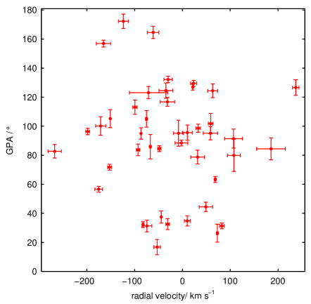
Figure 7: The GPA of the 44 bipolar PNe plotted against their Radial Velocities.The uncertainties forming the error bars for the radial velocities are taken from the catalogues. The figures for the polar and non-polar PNe are available online.

Some caution is required when considering this analysis in that the angles were measured in the plane of the sky and no adjustment to allow for projection effects was attempted. We do not have the additional data to derive the extent of the PNe along the line of sight. The fact that the data is two dimensional has two effects: First, it raises the possibility that some bipolar PNe were observed approximately along the lobes and consequently misclassified. Secondly, if we consider the angles of the PNe taken from the Galactic North Pole, through the lobe-to-lobe axis of PN towards the Galactic Plane the true angles will be more concentrated towards 90°. This can readily be seen by considering the GPA as lying on the diagonal of the front (rear) face of a cuboid with the PN stretching from the bottom right of that face to the top left of the rear (front) face see Fig. 8. From the figure we can see that:

$$r\cos\theta=l\cos\psi$$ (1)

$$r\sin\alpha\sin\theta=l\sin\psi$$ (2)

and

$$l\leq r$$ (3)

where $l$ and $r$ are the observed and actual lengths of the PN, and $\psi$, $\theta$ and $\alpha$ are the GPA, the angle from Galactic North to the axis of the PN and the angle of the axis of the PN projected onto the Galactic Plane from the PN’s Galactic longitude, respectively. We also have

$$r\leq r_{max}$$ (4)

where $r_{max}$ is the maximum permitted PN length of 35 arcsec, see §2. From equation 1 we can see that the value of the angle from Galactic North to the PN axis is closer to 90°than is the GPA.

Due to the rotation of the Bulge it seems reasonable to assume that the orientations of the projections onto the Galactic Plane are random. We created 100 000 possible samples based on our bipolar samples where, for each sample, the true length of each PN was estimated based on a random angle in the range [0,180) degrees that was taken as the (axial) orientation of its projection onto the Galactic Plane. Equations 1 to 3, the PN’s GPA and its projected length on the sky, and the maximum permitted PN length were used to ensure the validity of the angle on the Plane. We used the measured PN lengths of Rees, Zijlstra and Gesicki (in preparation) and the maximum permitted PN length of 35 arcsec (neither the observed nor maximum length changes due to the change in coordinates). The process was repeated for each PN until a ‘valid’ angle on the Plane was obtained whereupon the value of $\theta$ obtained from equation 1 was used as the angle from Galactic North down to the axis of the PN. The randomness of the angles in the sample was then checked using the same tests as in §3. The results are shown in Table 7 and suggest that the distribution of the angles from North is not random. Note that this process did not involve bootstrapping. Histograms of the derived angles are provided online.

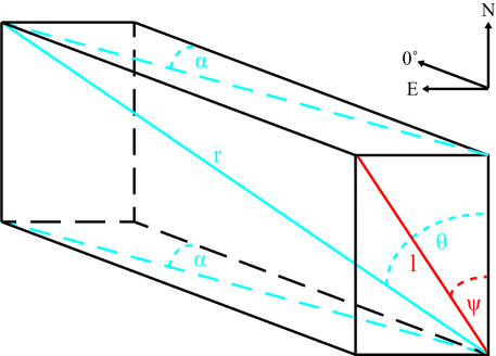
Figure 8: A schematic of the 3D situation. The axis of the PN is denoted by the blue line, its length by r and the angle from Galactic North to the axis by $\theta$. The projection onto the sky has its axis denoted by the red line, its length by l and the GPA by $\psi$. The projection onto the Galactic Plane is shown by the dotted blue line and its angle from 0°by $\alpha$. That line and its angle are repeated on the top face of the cuboid to clarify the derivation of the angle in the text. Similar schematics are valid for a PN with $\psi>90\degr$ and/or $\alpha>90\degr$.

Table 7: The p–values for the deprojected angles from Galactic North to the axes of the bipolar PNe sample. They are for 100 000 samples made up as follows. A random angle in the range [0,180) degrees was produced for each PN and used as the (axial) orientation when projection onto the Galactic Plane. The equations in §4 together with the PN’s GPA, its projected length on the sky as measured from the observations, and a maximum permitted ‘true’ PN length of 35 arcsec, see §2, were used to ensure the validity of the angle on the Plane. The process was repeated until a ‘valid’ angle on the Plane was obtained whereupon the angle from Galactic North down to the axis of the PN obtained from equation 1 was used as the sample value for the PN. The null hypothesis (H₀) for all the tests is that the distribution of the angles of the nebular axes from Galactic North is uniform. Quoted uncertainties in the statistics are based on the distribution of 100 subsamples of size 1 000 where that distribution is judged to be Normal using an Anderson–Darling test at a 0.5 significance level. The mean angle from Galactic North was estimated as $91.10\pm 0.04$°.

test	mean		standard		quantiles
			deviation		median		16%		84%
Rayleigh	$3\times 10^{-6}$		$5\times 10^{-6}$		8.	3$\pm 0.6\times 10^{-7}$	1.	2$\pm 0.1\times 10^{-7}$	4.	3$\pm 0.3\times 10^{-6}$
H1: non-uniform
Hodges-Ajne	1.	5$\pm 0.1\times 10^{-4}$	3.	9$\pm 0.6\times 10^{-4}$	$3\times 10^{-5}$		$4\times 10^{-6}$		$1\times 10^{-4}$
Kuiper	7.	1$\pm 0.4\times 10^{-6}$	1.	4$\pm 0.1\times 10^{-5}$	2.	3$\pm 0.2\times 10^{-6}$	$3\times 10^{-7}$		1.	22$\pm 0.08\times 10^{-5}$
Watson U2	$6\times 10^{-5}$		2.	5$\pm 0.2\times 10^{-4}$	$<10^{-7}$		$<10^{-7}$		$<10^{-7}$
Rayleigh	$2\times 10^{-7}$		$4\times 10^{-7}$		$6\times 10^{-8}$		$9\times 10^{-9}$		3.	3$\pm 0.03\times 10^{-7}$
H1: unimodal, $90^{\circ}$ mean

5 Discussion

5.1 Alignment

We divide the sample of PNe into three separate morphological categories. The statistics tell us that one of those categories, the bipolar PNe, shows evidence for alignment with the Galactic Plane while the other two appear to have random alignments. Our result for the bipolar PNe appears to be in reasonable conformity with that for the elongated PNe in the Galactic Centre region of Weidmann & Díaz (2008).

The GPA of the full sample of 130 PNe has an uniform distribution even with a significance level of 0.01 as used by Weidmann & Díaz (2008). This is also true for the samples of 55 polar, 31 non-polar and 86 elliptical (combined polar and non-polar) PNe and is the case for all the statistical tests for uniformity, see Tables 2 and 4.

A different result arises when we consider the bipolar subsample. If we restrict ourself to the measured values with no added uncertainties and no bootstrapping (Table 2), the Kuiper and Rayleigh tests for uniformity against a simple non-uniform alternative allow us to reject the null hypothesis of uniformity of the sample at a 0.001 significance level, the Watson U² test does so at the 0.01 level.

The Hodges-Ajne test does not let us reject uniformity. That test counts numbers on arbitrary semi-circles on the full circle and checks for an excess on one side. It has low resolution for a sample size of 44 as an increase or decrease of 1 in the minimum number on a semicircle can cause a large change in the p–value. A minimum of 11 angles on the semicircle produces a p–value of 0.02 whereas values of 10 and 12 produce p–values of 0.01 and 0.05 respectively. In effect there is a problematical step change in the p–values. The test also has higher standard deviations for the p–values than do the other tests for all the categories in Tables 3, 6 and 5. This suggests that it has less discriminatory value than other tests and we therefore place more weight on the results from them.

The Rayleigh tests for uniformity against the alternative of an unimodal distribution with mean values of 90° (i.e. along the Galactic Plane) and 100° both produce p–values below 0.0002. Fisher (1995) points out that tests with a simple non-uniformity alternative may not be very good at detecting something specific like unimodality whereas a test designed to detect that attribute may not be very good at detecting other types of non-uniformity. This difference might explain the difference in the results. The finger plots and rose plots of the bipolar sample indicate that it is reasonable to make an assumption of unimodality for it, which supports the use of the Rayleigh test against unimodal distributions.

The median p–values given in Table 4 confirm the basic result. Two of the tests for uniformity against a simple non-uniform alternative allow us to reject the null hypothesis of uniformity of the bipolar sample at the 0.001 (99.9 per cent) significance level and the other two do so at the 0.01 (99 per cent) significance level. The Rayleigh tests for uniformity against unimodal distributions with mean values of 90°and 100°both allow us to reject the null hypothesis of uniformity of the bipolar sample at the 0.0002 (99.98 per cent) significance level.

We did not pursue the results for any of the area subsamples using bootstrapping. However, the basic results, shown in Table 2, suggest that the non-random nature of the orientations is not due to some localized subset of the bipolar PNe. At the 0.01 significance level, the Rayleigh, Kuiper and Watson U² tests indicate that the orientations of the bipolar PNe are not random for either the West or North subsamples. The Rayleigh tests for uniformity against the alternative of an unimodal distribution with mean values of 90° (i.e. along the Galactic Plane) and 100°  also permit us to reject uniformity for some of the bipolar area subsamples at that significance level. We can do so for the West, North, North East and South West subsamples for both those mean orientations and for the South and East subsamples for the 90° mean orientation.

Corradi, Aznar & Mampaso (1998) found little evidence for alignments of PNe within the Galaxy. However, their sample of 209 PNe were spread around the Galaxy in terms of Galactic longitude and contained only 12 Bulge PNe. Weidmann & Díaz (2008) found an excess of elongated PNe toward the Galactic Centre that are oriented at 100°. As our sample and theirs have only 19 objects in common, of which only five are bipolar in our classification, we have an independent test of a potential alignment. We have restricted our study to PNe in the Bulge and, having taken the factors listed above into account, we consider that there is evidence that the GPA of the bipolar PNe in the Galactic Bulge do not have an uniform distribution. That is, that the two-dimensional orientation of the bipolar PNe in the Galactic Bulge is not random. Moreover, we find evidence of an alignment with a mean approximately along the Galactic Plane.

PN orientations are expected to be independent of each other because a PN’s shape is set by processes internal to the originating star or stellar system. A mechanism is required.

5.2 Orientation Changes After PN Ejection

The velocity graphs in Fig. 7 together with the small Pearson product-moment correlation coefficients for the radial and expansion velocity regressions suggest that there is no relationship between PN orientation and either PN radial velocity or PN expansion velocity. Similarly, Fig. 6 together with low Pearson product-moment correlation coefficients suggest that there is no relationship between PN orientation and size. In particular, the plot for the bipolar PNe in Fig. 6 together with a Pearson product-moment correlation coefficient of -0.009 from a simple linear regression of the GPA against the PNe angular size from lobe tip to lobe tip, demonstrates that the orientation of bipolar PNe is not related to lobe length. The variation in distance to the PNe is unlikely to be such as to change that conclusion.

The lobe length of a bipolar PN is related to the age of the PN. The lack of relation between orientation and lobe length suggests that the orientation is set during the youth of the PN or before it has formed. There is no evidence that the orientation changes during the PN evolution. The expansion velocity tends to be higher for higher-mass central stars (although this may not be important for the old stellar population of the Galactic Bulge), or for emission-line central stars (Gesicki et al., 2006). These aspects are not shown to be related to the orientation. We also found no evidence that orientation is related to radial velocity.

It has been suggested that magnetic fields in the interstellar medium (ISM) elongate stellar wind bubbles and that this is important in the production of bilateral supernova remnants (Gaensler, 1998). In the case of PNe however, that magnetic field can have little effect during the formation of the nebula due to the small size scales involved (the wind acceleration region is located within 1–10 AU from the star) and the high densities in the wind. Moreover, this mechanism would not explain why the alignment is found only for bipolar PNe.

5.3 Angular momentum

The currently favoured view for shaping non-spherical PNe is that of binary interactions (de Marco, 2009) . In this model, either an AGB star provides spherical ejecta and its interactions with a binary companion shapes those ejecta, or a close binary forms a common envelope leading to aspherical ejecta (Zijlstra, 2007). Stellar magnetic fields also provide possible shaping mechanisms, however Soker (2006) argues that sufficiently strong fields still require a companion to continuously spin up the envelope.

The distinction between bipolar and other PNe is likely related to the amount of angular momentum available for shaping. The angular momentum available for shaping is set by a balance between the orbital angular momentum and the efficiency of the transfer of momentum. Bipolar nebulae show dense tori which shape the polar flows. They may arise from intermediate $\left(\sim\!1~{}\mathrm{yr}\right)$ and short-period $\left(\leq 0.1~{}\mathrm{yr}\right)$ binaries. Shorter period binaries form common-envelope systems and nebulae ejected by them often show thin rings rather than dense tori (Zijlstra, 2007), possibly related to the lower angular momentum available in close systems. For common envelope systems the momentum transfer efficiency will be 100%; the percentage is lower for wider systems. The widest binaries $\left(\gtrsim 10~{}\mathrm{yr}\right)$ show spiral features but do not form bipolar nebulae (Maercker et al., 2012).

Although the orbit of a star around the Galaxy may change due to interactions with other bodies, the angular momentum vector of the stellar system tends to remain stable. The Kozai–Lidov mechanism (a three-body interaction) (Shappee & Thompson, 2013) could prevent the retention of any alignment of binary systems that occurs during the early stages of star formation i.e. it could randomize the alignments. However, any method of alignment of the PNe in the later stages of the lives of the systems that form them would then be required to operate over kiloparsec distances and appears implausible. Consequently, given that we have found an alignment, that alignment must have originated during the formation of the stars.

5.4 A proposed mechanism

The dense molecular clouds within about 4° of the Galactic centre tend to have their magnetic fields aligned along the Galactic plane (Morris, 1998) and these fields are quite uniform and strong. If that was also the case for the Bulge at the time of its star formation, a propensity for the stars which form the bipolar PNe to align with the magnetic field of the cloud from which they themselves are formed could provide an explanation for the non-random distribution of the PNe orientations.

A strong magnetic field embedded in a star-forming cloud slows the contraction of star-forming cores along the direction perpendicular to the magnetic field (Tang et al., 2009). The material around the collapsing young stellar objects may be expected to contract more quickly along the magnetic field. If a binary forms in the thus-flattened cloud, the separation will on average be larger perpendicular to the field. As wider binaries carry more angular momentum, this gives a preferential angular momentum vector of the binary population along the magnetic field. So the stronger the field, the greater is the propensity towards forming wide binaries with orbits perpendicular to that field. Whether this occurs in reality is controversial. Hydrodynamical models indicate that for larger fields $\left(\sim 80~{}\mu\mathrm{G}\right)$, outflows indeed become oriented along the magnetic field lines (Matsumoto, Nakazato & Tomisaka, 2006). Also, the 3D MHD simulations of Nakamura & Li (2008) appear to show that star formation in relatively diffuse clouds containing strong magnetic fields is controlled by those fields, not by turbulence.

The evidence for orientation of stellar rotation axes along interstellar magnetic field lines in nearby-clusters is not conclusive. While the T Tauri stars FU Ori and DR Tau have their stellar axes aligned with the larger magnetic field direction (Vink et al., 2005), other studies suggest that the orientation of young stellar objects in a cluster is random (Ménard & Duchêne, 2004; Jackson & Jeffries, 2010). However, no studies have been made on possible alignment of binary orbits within young clusters. Binary orbits carry far more angular momentum than does stellar rotation, and the result from the Galactic Bulge PNe could indicate that the alignment survives only in binary systems. We can also not exclude the possibility that magnetic fields within the Bulge during its formation were considerable stronger than those in the Solar neighbourhood. Matsumoto, Nakazato & Tomisaka (2006) show that the strength of the field is an important parameter, with alignment occurring above 80 $\mu\mathrm{G}$.

The alignment of bipolar PNe suggests that there was an alignment of stellar systems in the Bulge at the time of the formation of the stars, most clearly seen for those objects with the largest angular momentum. That alignment lies approximately along the Galactic plane. This implies that the binary systems in the Galactic Bulge have angular momentum vectors that are preferentially aligned along the Galactic plane. There is strong evidence for cylindrical rotation in the Bulge, with angular momentum perpendicular to the Galactic plane (Howard et al., 2009). We thus have the counter-intuitive situation that binary systems out of which bipolar PNe are formed have their angular momentum vector perpendicular to that of the Bulge in which they formed.

In conclusion, we have evidence that the orientation of bipolar PNe in the Bulge is not random. The argument that we use is that the angular momentum vectors are aligned. This effect is likely to date from the origin of the central stars of the PNe. Interstellar magnetic fields at the time of the formation of the Bulge provide a possible mechanism.

6 Summary

We have classified 130 PNe that we consider to be in the Galactic Bulge into three morphological categories. For each of those PNe, we determined a position angle for the polar direction and converted that to an angle from Galactic north to Galactic east. We then undertook a statistical analysis of those angles and found that for one of the morphological classes, the bipolar class, there is evidence for a non-random distribution of the angles at significance levels equivalent to that between $2.3\sigma$ and $3.7\sigma$ (depending on the test used) for a Gaussian distribution. The mean orientation is aligned approximately to that of the galactic plane. On the basis that the orientation of the bipolar nebulae is independent of their size we propose a mechanism for the production of that non-random distribution of orientations.

The debate on the main shaping mechanism in PNe has concentrated on binarity and magnetic fields. Currently, binary systems are seen as the dominant effect (this may be of course be influenced by the fact that binaries are easier to detect than magnetic fields), with magnetic fields having a secondary role. The hypothesis put forward in this paper is that the alignment of bipolar planetary nebulae can be understood if star formation in the Bulge occurred in the presence of strong magnetic fields oriented along the Galactic plane and if the parameters of the binary systems themselves are in part the product of magnetic fields present at their origin. This reverses again cause and effect. The long debate has shown that both effects are difficult to separate, and are to a significant degree intertwined.The estimated ages of stars in the Bulge vary with estimates from 8 to $\sim\!13$ Gyr (Rich, 2001; Minniti & Zoccali, 2008; Bensby et al., 2010). The claim in this paper is that this interaction between field and binarity dates back to the processes acting during the origin of the stars, a form of archaeomagnetism of the early Universe.

We are of the view that a similar analysis should be performed on high resolution observations of a much larger sample of bipolar PNe in the Galactic Bulge.

References

- Acker et al. (1992) Acker A., Marcout J., Ochsenbein F., Stenholm B., Tylenda R., 1992, Strasbourg - ESO catalogue of galactic planetary nebulae. Part 1; Part 2. Garching: European Southern Observatory
- Acker, Peyaud & Parker (2006) Acker A., Peyaud A. E. J., Parker Q., 2006, in Barlow M. J., Méndez R. H., eds., IAU Symposium, Vol. 234, Planetary Nebulae in our Galaxy and Beyond, p. 355
- Balick & Frank (2002) Balick B., Frank A., 2002, ARA&A, 40, 439
- Beaulieu, Dopita & Freeman (1999) Beaulieu S. F., Dopita M. A., Freeman K. C., 1999, ApJ, 515, 610
- Bensby et al. (2010) Bensby T. et al., 2010, A&A, 512, A41
- Berens (2009) Berens P., 2009, Journal of Statistical Software, 31, 1
- Blackman (2009) Blackman E. G., 2009, in Strassmeier K. G., Kosovichev A. G., Beckman J., eds., IAU Symposium, Vol. 259, Cosmic Magnetic Fields: from Planets, to Stars and Galaxies, p. 35
- Bogdan, Bogdan & Futschik (2002) Bogdan M., Bogdan K., Futschik A., 2002, Annals of the Institute of Statistical Mathematics, 54, 29