Breaking entanglement-breaking by classical correlations

Abstract

The inevitable interaction between quantum systems and environment induces effects of decoherence which may be so strong as to destroy any initial entanglement between the systems, a phenomenon known as “entanglement breaking”. Here we show the simplest examples where the combination of two entanglement-breaking channels into a joint correlated-noise environment reactivates the distribution of entanglement, with classes of entangled states which are perfectly transmitted from a middle station (Charlie) to two remote stations (Alice and Bob). Surprisingly, this reactivation is induced by the presence of purely-classical correlations in the joint environment, whose state is separable with zero discord. This paradoxical effect is proven for quantum systems with Hilbert spaces of any dimension, both finite and infinite.

I Introduction

The distribution of entanglement is a central topic of investigation in the quantum information community. Unfortunately, this distribution is also fragile: Quantum systems inevitably interact with the external environment whose decoherent action typically degrades their entanglement. The worst scenario is when decoherence is so strong as to destroy any input entanglement. Mathematically, this situation is represented by the concept of entanglement-breaking channel EBchannels ; HolevoEB . In general, a quantum channel $\mathcal{E}$ is entanglement-breaking when its local action on one part of a bipartite state always results into a separable output state. In other words, given two systems, $A$ and $B$, in an arbitrary bipartite state $\rho_{AB}$, the output state $\rho_{AB^{\prime}}=(\mathcal{I}_{A}\otimes\mathcal{E}_{B})(\rho_{AB})$ is always separable, where $\mathcal{I}_{A}$ is the identity channel applied to system $A$ and $\mathcal{E}_{B}$ is the entanglement-breaking channel applied to system $B$.

Despite entanglement-breaking channels having been the subject of an intensive study by the community, they have only been analyzed under Markovian conditions of no memory. In other words, when the distribution involves two or more systems, these systems are typically assumed to be perturbed in an independent fashion, each of them subject to the same memoryless channel. For instance, consider the scheme depicted in panel (1) of Fig. 1, where a middle station (Charlie) has a bipartite system $AB$ in some entangled state, but its communication lines with two remote parties (Alice and Bob) are affected by entanglement-breaking channels $\mathcal{E}_{A}$ and $\mathcal{E}_{B}$.

Under the assumption of memoryless channels, there is clearly no way to distribute entanglement among any of the parties. Suppose that Charlie tries to share entanglement with one of the remote parties by sending one of the two systems while keeping the other (a scenario that we call “1-system transmission” or just “single transmission”). For instance, Charlie may keep system $A$ while transmitting system $B$ to Bob. The action of $\mathcal{I}_{A}\otimes\mathcal{E}_{B}$ destroys the initial entanglement, so that systems $A$ (kept) and $B^{\prime}$ (transmitted) are separable. Symmetrically, the action of $\mathcal{E}_{A}\otimes\mathcal{I}_{B}$ destroys the entanglement between system $A^{\prime}$ (transmitted) and system $B$ (kept). Now suppose that Charlie sends system $A$ to Alice and system $B$ to Bob (a scenario that we call “2-system transmission” or “double transmission”). Since the joint action of the two channels is given by the tensor product $\mathcal{E}_{A}\otimes\mathcal{E}_{B}=(\mathcal{E}_{A}\otimes\mathcal{I}_{B})(\mathcal{I}_{A}\otimes\mathcal{E}_{B})$ quantum entanglement must necessarily be destroyed. In other words, since we have 1-system entanglement-breaking, then we must have 2-system entanglement-breaking.

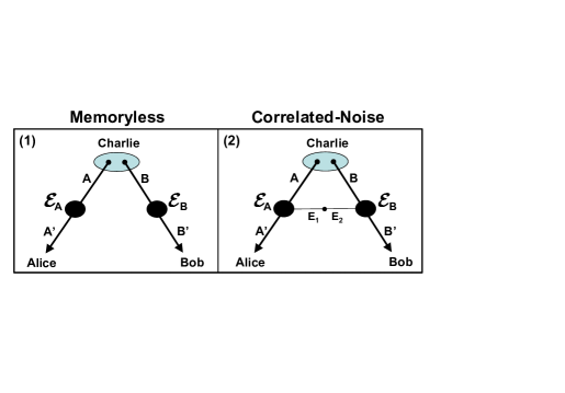
Figure 1: Symmetric scheme for entanglement distribution in memoryless (1) and correlated-noise (2) environments. Charlie is the middle station with an entangled state of systems $A$ and $B$. Alice and Bob are the remote receiving stations. Charlie may choose to keep one system and send the other to Alice or Bob (single transmission) or he may decide to send both the systems to the remote stations (double transmission). In panel (1) we consider two memoryless entanglement-breaking channels, $\mathcal{E}_{A}$ and $\mathcal{E}_{B}$. No entanglement can be distributed, neither via single transmission (Charlie $\rightarrow$ Alice or Charlie $\rightarrow$Bob), nor via double transmission (Charlie $\rightarrow$ Alice and Bob). In panel (2) we consider the presence of correlations between the two entanglement-breaking channels. In this scenario, despite entanglement cannot be distributed by single transmission (Charlie cannot be entangled with Alice or Bob), still it can be distributed via the double transmission (so that Alice and Bob can become entangled). This reactivation of entanglement distribution is possible in the presence of classical correlations, i.e., for an environment (systems $E_{1}$ and $E_{2}$) in a purely-classical state (separable, with zero-discord).

In this paper we show that the previous implication is false when we introduce correlations (i.e., a memory) between the two entanglement-breaking channels. In other words, in the presence of correlated-noise environments, the double transmission can successfully distribute entanglement despite the single transmission being subject to entanglement-breaking. This is equivalent to say that Charlie can transmit entanglement to Alice and Bob, despite not being able to share any entanglement with them. The most interesting fact is that the entanglement distribution via the double transmission is reactivated by the presence of separable and purely-classical correlations in the joint environment. This effect is proven for quantum systems with Hilbert spaces of any dimension, both finite (qudits) and infinite (continuous variable systems BraREV2 ; RMP ).

In particular, here we are interested in showing the simplest examples of correlated-noise environments which allow for a perfect distribution of entanglement via the double transmission (2-system entanglement-preserving) while preventing any entanglement distribution via the single transmission (1-system entanglement-breaking). These environments are constructed by using the so-called twirling operators $U\otimes U$ (or $U\otimes U^{\ast}$). A random unitary $U$ is applied to system $A$ and the same unitary (or its conjugate) is applied to system $B$. While the local action of a random unitary ($U\otimes I$ or $I\otimes U$) is entanglement-breaking, the correlated action ($U\otimes U$) perfectly preserves specific classes of entangled states (belonging to decoherent-free subspaces of the joint correlated environment).

Since these “twirling environments” are based on local operations and classical communication (LOCC), they are expected to introduce correlations which are separable (local) and, more precisely, purely-classical. This feature can be checked by considering a unitary dilation where an explicit system for the environment is introduced. For the twirling environments, such a system can be described by a classical state, i.e., separable with zero quantum discord.

Twirling environments can easily be constructed for quantum systems of any dimension. In the case of two qudits (each with Hilbert space of dimension $d$), the randomization of the twirling operators $U\otimes U$ (or $U\otimes U^{\ast}$) is performed over the entire unitary group. In this case, it is easy to identify states which are invariant under $U\otimes U$-twirling (Werner states Werner ) and $U\otimes U^{\ast}$-twirling (isotropic states HOROs ). In the specific case of qubits ($d=2$), we can restrict the randomization to the basis of the Pauli operators, with the qubit Werner state being invariant under Pauli twirling. Things are less trivial for infinite dimension, in particular, for bosonic modes. In this case, we restrict the twirling operators to the compact group of orthogonal symplectic transformations, i.e., phase-space rotations. The bosonic twirling environment so defined is non-Gaussian. It is interesting to see that, only for the $U\otimes U^{\ast}$-twirling, we can identify Gaussian states which are invariant and entangled: These are the two mode squeezed vacuum states, also known as Einstein-Podolsky-Rosen (EPR) states EPR ; RMP .

In terms of potential impact, our work opens new possibilities for entanglement distribution in correlated-noise environments and memory channels, where the presence of correlations can be exploited to recover from entanglement breaking. Since entanglement recovery can be achieved by the injection of separable purely-classical correlations, our work poses fundamental questions on the intimate relations between local and nonlocal correlations and, more generally, between classical and quantum correlations.

The paper is structured as follows. In Sec. II, we consider qubits and we show the simplest twirling environments (correlated Pauli environments). In Sec. III, we consider the general case of qudits evolving in multidimensional twirling environments. These results can also be applied to the case of qubits. Then, in Sec. IV, we consider bosonic systems and their evolution under non-Gaussian twirling environments which are based on correlated phase-space rotations. Finally, Sec. V is for conclusion, with a number of Appendices A, B, C, D and E containing simple proofs and technical details.

II Qubits in correlated Pauli environments

The most strikingly simple example can be constructed for qubits considering the basis of the four Pauli operators $I$, $X$, $Y=iXZ$ and $Z$ Nielsen . Given an arbitrary input state $\rho_{AB}$ of two qubits, we consider the correlated Pauli channel

$$\mathcal{E}(\rho_{AB})=\sum_{k=0}^{3}p_{k}~{}(P_{k}\otimes P_{k})\rho_{AB}(P_{k}\otimes P_{k})^{\dagger}~{},$$ (1)

where $P_{k}\in\{I,X,Y,Z\}$ and $p_{k}$ are probabilities. This channel is clearly simulated by random LOCCs. In fact, it is equivalent to extract a random variable $K=\{k,p_{k}\}$, apply the Pauli unitary $P_{k}$ to qubit $A$, communicate $k$ and then apply the same unitary $P_{k}$ to qubit $B$. It is easy to check that the two-qubit channel of Eq. (1) does not change if we replace the Pauli twirling operator $P_{k}\otimes P_{k}$ with the alternative operator $P_{k}\otimes P_{k}^{\ast}$.

It is easy to write the unitary dilation of the correlated Pauli channel. It is sufficient to introduce an environment composed by two systems $E_{1}$ and $E_{2}$, each being a qudit with dimension $d=4$ and orthonormal basis $\{\left|k\right\rangle\}_{k=0}^{3}$. Then, we can write

$$\mathcal{E}(\rho_{AB})=\mathrm{Tr}_{E_{1}E_{2}}\left[U(\rho_{AB}\otimes\rho_{E_{1}E_{2}})U^{\dagger}\right]~{},$$ (2)

where the environment is prepared in the correlated state

$$\rho_{E_{1}E_{2}}=\sum_{k=0}^{3}p_{k}\left|k\right\rangle_{E_{1}}\left\langle k\right|\otimes\left|k\right\rangle_{E_{2}}\left\langle k\right|~{},$$ (3)

and the unitary interaction $U=U_{E_{1}A}\otimes U_{E_{2}B}$ is a tensor product of two control-Pauli unitaries,

$$U_{E_{1}A}=\sum_{k=0}^{3}\left|k\right\rangle_{E_{1}}\left\langle k\right|\otimes P_{k},~{}U_{E_{2}B}=\sum_{k=0}^{3}\left|k\right\rangle_{E_{2}}\left\langle k\right|\otimes P_{k}.$$ (4)

As evident from Eq. (3), the state of the environment is separable, which means that only separable (i.e., local-type) correlations are injected into the travelling qubits. More precisely, since $\rho_{E_{1}E_{2}}$ is expressed as a convex combination of orthogonal projectors, it is a purely-classical state, i.e., a state with zero quantum discord RMPdis . As a result, this environment contains correlations which are not only local but also purely classical.

Now we show the conditions under which the correlated Pauli environment is simultaneously one-qubit entanglement-breaking and two-qubit entanglement preserving. We start by considering the transmission of one qubit only, e.g., qubit $A$. In this case, Eq. (1) reduces to a depolarizing channel

$$(\mathcal{E}_{A}\otimes\mathcal{I}_{B})(\rho_{AB})=\sum_{k=0}^{3}p_{k}(P_{k}\otimes I)\rho_{AB}(P_{k}^{\dagger}\otimes I)$$

$$=p_{0}\rho_{AB}+\sum_{k=1}^{3}p_{k}(P_{k}\otimes I)\rho_{AB}(P_{k}^{\dagger}\otimes I).$$ (5)

It is easy to show that $\mathcal{E}_{A}$ is entanglement-breaking when $p_{k}\leq 1/2$ for any $k$ (see Appendix A for a simple proof). A particular choice can be $p_{0}\leq 1/2$ and $p_{1}=p_{2}=p_{3}=(1-p_{0})/3$ as for instance used in Ref. Sacchi .

Assuming the condition of one-qubit entanglement-breaking ($p_{k}\leq 1/2$), Charlie is clearly not able to share any entanglement with Alice or Bob. Can he still distribute entanglement to Alice and Bob? Yes, this is possible because we can identify a class of entangled states which are invariant under the action of the correlated map (1). This class is simply given by the Werner states

$$\rho_{AB}(\gamma):=(1-\gamma)\frac{I_{AB}}{4}+\gamma\left|-\right\rangle_{AB}\left\langle-\right|~{},$$ (6)

with parameter $-1/3\leq\gamma\leq 1$, where $I_{AB}/4$ is the maximally-mixed state and

$$\left|-\right\rangle_{AB}=\frac{1}{\sqrt{2}}\left(\left|0\right\rangle_{A}\left|1\right\rangle_{B}-\left|1\right\rangle_{A}\left|0\right\rangle_{B}\right)$$ (7)

is the maximally-entangled (singlet) state. For $\gamma>1/3$, the two-qubit state $\rho_{AB}(\gamma)$ is known to be entangled and distillable. Since qubit Werner states are invariant under any twirling operator $U\otimes U$, i.e.,

$$(U\otimes U)\rho_{AB}(\gamma)(U\otimes U)^{\dagger}=\rho_{AB}(\gamma)~{},$$ (8)

for any unitary $U$, they are fixed points of the correlated map (1) or, in other words, they represent a decoherence-free subspace of the correlated Pauli environment. Thus, if Charlie sends Werner states with $\gamma>1/3$, these entangled states are perfectly distributed to Alice and Bob (two-qubit entanglement preserving).

III Qudits in multidimensional twirling environments

In this section we consider quantum systems whose Hilbert space has finite dimension $d$, i.e., qudits (in particular, we have qubits for $d=2$). For these systems, we can easily construct classically-correlated environments which are simultaneously 1-qudit entanglement-breaking and 2-qudit entanglement-preserving.

Consider two qudits, $A$ and $B$, with same dimension $d$ and prepared in a bipartite state $\rho_{AB}$. Then, we call $U\otimes U$ twirling channel the following completely positive trace-preserving map

$$\mathcal{E}_{UU}(\rho_{AB})=\int_{\mathcal{U}(d)}dU~{}(U\otimes U)\rho_{AB}(U\otimes U)^{\dagger}~{},$$ (9)

where the integral is over the entire unitary group $\mathcal{U}(d)$ acting on the $d$-dimensional Hilbert space, and $dU$ is the Haar measure. This channel is clearly realizable by random LOCCs. In fact, it is equivalent to choose a random unitary $U$, apply it to the local system $A$, and then apply the same $U$ to the other local system $B$ (where the coordination of the two local unitaries is mediated by classical communication). Similarly, we can define a $U\otimes U^{\ast}$ twirling channel, by replacing the twirling operator $U\otimes U$ with the alternative twirling $U\otimes U^{\ast}$ in the definition of Eq. (9). Compactly, we refer to the $U\otimes V$ twirling channel

$$\mathcal{E}_{UV}(\rho_{AB})=\int_{\mathcal{U}(d)}dU~{}(U\otimes V)\rho_{AB}(U\otimes V)^{\dagger}~{},$$ (10)

where $V=U$ or $V=U^{\ast}$.

In order to study its correlation properties we dilate this channel into an environment. Note that, since we have an integral in Eq. (10), the dilation of the channel seems to involve the introduction of continuous variable systems. In fact, the unitary group $\mathcal{U}(d)$ is described by $d^{2}$ real parameters UnitaryPAR , which means that we would need to employ $d^{2}$ continuous variable systems for the environment. Actually, this continuous dilation is not necessary, since can always replace the previous Haar integral with a discrete sum over a finite number of suitably-chosen unitaries. In fact, any twirling channel (10) can be written as

$$\mathcal{E}_{UV}(\rho_{AB})=\frac{1}{K}\sum_{k=0}^{K-1}(U_{k}\otimes V_{k})\rho_{AB}(U_{k}\otimes V_{k})^{\dagger}~{},$$ (11)

where $U_{k}$ belongs to the set of unitary 2-design $\mathcal{D}$ Designs ; Des2 and $V_{k}=U_{k}$ or $V_{k}=U_{k}^{\ast}$. The set $\mathcal{D}$ has a finite number of elements which depends of the dimension of the Hilbert space $K=K(d)$ (too see how the cardinality $K$ scales with the dimension $d$, see for instance Ref. Gross ). The proof of the equivalence between Eqs. (10) and (11) can be found in Ref. Designs for the $U\otimes U$ twirling channel. See Appendix B for a simple extension of the proof to the other $U\otimes U^{\ast}$ twirling channel. Note that, in the case of qubits ($d=2$), an example of unitary 2-design is provided by the Clifford group Designs ; Clifford3 , which is the normalizer of the Pauli group and typically employed in quantum error correction Clifford1 ; Clifford2 .

Now using the unitary 2-design, we can dilate the twirling channel into an environment made by finite-dimensional systems, i.e., two larger qudits $E_{1}$ and $E_{2}$, each with dimension $K$ and orthonormal basis $\{\left|k\right\rangle\}_{k=0}^{K-1}$. In fact, we can write

$$\mathcal{E}_{UV}(\rho_{AB})=\mathrm{Tr}_{E_{1}E_{2}}\left[U(\rho_{AB}\otimes\rho_{E_{1}E_{2}})U^{\dagger}\right]~{},$$ (12)

where the environment is prepared in the uniformly correlated state

$$\rho_{E_{1}E_{2}}=\frac{1}{K}\sum_{k=0}^{K-1}\left|k\right\rangle_{E_{1}}\left\langle k\right|\otimes\left|k\right\rangle_{E_{2}}\left\langle k\right|~{},$$ (13)

and the unitary interaction $U=U_{E_{1}A}\otimes U_{E_{2}B}$ is a tensor product of two control-unitaries

$$U_{E_{1}A}=\sum_{k=0}^{K-1}\left|k\right\rangle_{E_{1}}\left\langle k\right|\otimes U_{k},~{}U_{E_{2}B}=\sum_{k=0}^{K-1}\left|k\right\rangle_{E_{2}}\left\langle k\right|\otimes V_{k},$$ (14)

where $U_{k}\in\mathcal{D}$ and $V_{k}=U_{k}$ or $V_{k}=U_{k}^{\ast}$. As evident from Eq. (13), the state of the environment is separable and purely-classical (zero discord). In other words, twirling environments only contain purely-classical correlations.

Once we have characterized the correlation properties of these environments, we show the conditions under which they are simultaneously one-qudit entanglement-breaking and two-qudit entanglement preserving. First of all, let us explicitly show that one-qudit transmission is always subject to entanglement breaking. Suppose that only qudit $A$ is transmitted by Charlie. Then, for any input state $\rho_{AB}$, the output state of Alice and Charlie is given by

$$(\mathcal{E}_{A}\otimes\mathcal{I}_{B})(\rho_{AB}) =$$

$$\int_{\mathcal{U}(d)}dU~{}(U\otimes I)\rho_{AB}(U^{\dagger}\otimes I) =\frac{1}{d}I\otimes\mathrm{Tr}_{A}(\rho_{AB})~{},$$ (15)

which means that the random map $U\otimes I$ represents an entanglement-breaking channel (similar result holds for the other random map $I\otimes V$ involved in the transmission of the other qudit $B$). As shown in Appendix C, the proof of Eq. (15) is a simple application of the identity

$$\left\langle O\right\rangle_{U}:=\int_{\mathcal{U}(d)}dU~{}UOU^{\dagger}=\frac{\mathrm{Tr}(O)}{d}I~{},$$ (16)

which is the Haar average of a linear operator $O$. In turn, Eq. (16) is a simple consequence of Schur’s lemma and the invariance of the Haar measure Chiri .

The next step is to consider two-qudit transmission from Charlie to Alice and Bob. In this case, we search for entangled states which are preserved by the correlated action of the twirling environment. Luckily, we can easily find states which are invariant under the action of the twirling operator $U\otimes V$, i.e.,

$$(U\otimes V)\rho_{AB}(U\otimes V)^{\dagger}=\rho_{AB}~{}.$$ (17)

Thanks to this invariance, such states are fixed points of the $U\otimes V$ twirling channel of Eq. (10).

In the specific case of $V=U$, it is well known that the unique solution of Eq. (17) is provided by the multidimensional Werner states, which are themselves defined as those states invariant under $U\otimes U$ twirling Werner . Given two isodimensional qudits, $A$ and $B$, their $d\times d$ Werner state is a one-parameter class defined by Werner ; Synak

$$\rho_{AB}(\mu):=\frac{1}{d^{2}+d\mu}(I_{AB}+\mu V)$$ (18)

where $-1\leq\mu\leq 1$ and $V$ is the unitary flip operator $V\left|\varphi\right\rangle_{A}\otimes\left|\psi\right\rangle_{B}=\left|\psi\right\rangle_{A}\otimes\left|\varphi\right\rangle_{B}$. This state is known to be entangled for $\mu<-d^{-1}$. Thus, if Charlie has a Werner state $\rho_{AB}(\mu)$ with suitable $\mu$ (in the entanglement regime), he is able to perfectly transmit his state to Alice and Bob, who can then share and distill entanglement. This entanglement distribution from Charlie to Alice and Bob is possible, despite Charlie cannot share any entanglement with the remote parties due to the entanglement breaking condition of Eq. (15).

Coming back to Eq. (17), one can find a similar solution for $V=U^{\ast}$. In fact, as shown in Ref. HOROs , there exist states which are invariant under $U\otimes U^{\ast}$-twirling. These are called isotropic states, and they are defined by the one-parameter class HOROs

$$\rho_{AB}(\gamma):=(1-\gamma)\frac{I_{AB}}{d^{2}}+\gamma\left|\psi\right\rangle_{AB}\left\langle\psi\right|~{},$$ (19)

where the maximally mixed state $d^{-2}I_{AB}$ and the maximally entangled state

$$\left|\psi\right\rangle_{AB}=\frac{1}{\sqrt{d}}\sum_{k=0}^{d-1}\left|k\right\rangle_{A}\left|k\right\rangle_{B}~{},$$ (20)

are combined with parameter $-(d^{2}-1)^{-1}\leq\gamma\leq 1$. In general, it is entangled and distillable for $\gamma>(1+d)^{-1}$. Thus, if Charlie has an isotropic state $\rho_{AB}(\gamma)$ with suitable $\gamma$ (i.e., in the entanglement regime), he is able to perfectly transmit this state to Alice and Bob, who therefore can share and distill entanglement. Again, this is possible despite the transmission of a single qudit is subject to an entanglement-breaking channel, as expressed by Eq. (15).

It is clear that these results can be specialized to the case of qubits ($d=2$). For qubits, the classes of multidimensional Werner states of Eq. (18) and isotropic states of Eq. (19) coincide up to a local unitary HOROs . Multidimensional Werner states reduce to the qubit Werner state of Eq. (6) which is $U\otimes U$-invariant. In fact, for $d=2$, we have $(I_{AB}+\mu V)=(\mu+1)I_{AB}-2\mu\left|-\right\rangle_{AB}\left\langle-\right|$ which, replaced in Eq. (18), gives the state of Eq. (6) by setting $\gamma=-\mu/(2+\mu)$.

On the other hand, isotropic states reduce to Eq. (6), proviso that the singlet $\left|-\right\rangle_{AB}$ is replaced by the triplet

$$\left|+\right\rangle_{AB}=\frac{1}{\sqrt{2}}\left(\left|0\right\rangle_{A}\left|0\right\rangle_{B}+\left|1\right\rangle_{A}\left|1\right\rangle_{B}\right)~{}.$$ (21)

This state is $U\otimes U^{\ast}$-invariant and known as Werner-like state. Since singlet and triplet states are connected by a local unitary, there is no difference in the quantum correlations which are contained in the state according to the two definitions. More generally, in a Werner-like state, any maximally entangled state could be considered in the place of the singlet.

IV Bosonic twirling environments

Here we extend the analysis to the case of continuous variable systems, i.e., quantum systems with infinite dimensional Hilbert spaces ($d=\infty$). In particular, we consider the case of two bosonic modes of the electromagnetic field. The simplest generalization of the notion of twirling environment involves the use of rotations in the phase space. Given a single bosonic mode with number operator $\hat{n}$, the rotation operator is defined as $\hat{R}_{\theta}=\exp(-i\theta\hat{n})$. In the phase space, the action of this operator is described by the well-known rotation matrix

$$\mathbf{R}_{\theta}=\left(\begin{array}[c]{cc}\cos\theta&\sin\theta\\ -\sin\theta&\cos\theta\end{array}\right)~{}.$$ (22)

In terms of the second-order statistical moments, we have that the covariance matrix (CM) $\mathbf{V}$ of the input mode is transformed via the congruence

$$\mathbf{V}\rightarrow\mathbf{R}_{\theta}\mathbf{VR}_{\theta}{}^{T}~{}.$$ (23)

Now, given an input state $\rho_{AB}$ of two modes, $A$ and $B$, we can synchronize two random rotations and define the bosonic twirling channel

$$\mathcal{E}_{\theta\theta^{\prime}}(\rho_{AB})=\int\frac{d\theta}{2\pi}~{}(\hat{R}_{\theta}\otimes\hat{R}_{\theta^{\prime}})\rho_{AB}(\hat{R}_{\theta}\otimes\hat{R}_{\theta^{\prime}})^{\dagger},$$ (24)

where $\theta^{\prime}=\theta$ or $\theta^{\prime}=-\theta$. This is a non-Gaussian channel, since the twirling operator $\hat{R}_{\theta}\otimes\hat{R}_{\theta^{\prime}}$, despite Gaussian, is not averaged using a Gaussian distribution but a uniform one. It is clearly based on random LOCCs, since random rotations are locally applied to each bosonic mode and they are correlated via classical communication.

It is interesting that the unitary dilation of this channel can be restricted to a finite-dimensional environment. The reason is because the single-mode rotation operator $\hat{R}_{\theta}$ belongs to the compact subgroup of the orthogonal symplectic transformations $\mathcal{K}(2)=\mathcal{S}p(2)\cap\mathcal{O}(2)$ (which are passive Gaussian unitaries, i.e., unitary transformations preserving both the Gaussian statistics and the energy of the state). Then, $\mathcal{K}(2)$ is isomorphic to the unitary group $\mathcal{U}(1)$, which is the multiplicative group composed by all complex numbers with module 1, also known as the circle group. For this reason, a unitary 2-design $\mathcal{D}\subset\mathcal{U}(1)$ can be mapped into a unitary 2-design for $\mathcal{K}(2)$ Gross . As a result, we can write

$$\mathcal{E}_{\theta\theta^{\prime}}(\rho_{AB})=\frac{1}{K}\sum_{k=0}^{K-1}(\hat{R}_{\theta_{k}}\otimes\hat{R}_{\theta_{k}^{\prime}})\rho_{AB}(\hat{R}_{\theta_{k}}\otimes\hat{R}_{\theta_{k}^{\prime}})^{\dagger},$$ (25)

for a suitable set of angles $\{\theta_{0},\ldots,\theta_{K-1}\}$ and where $\theta_{k}^{\prime}=\theta_{k}$ or $\theta_{k}^{\prime}=-\theta_{k}$. In this form, the channel is manifestly non Gaussian. Then, as before, it can be represented using two environmental qudits, $E_{1}$ and $E_{2}$, prepared in a correlated state $\rho_{E_{1}E_{2}}$ as in Eq. (13) and interacting with the two bosonic modes via two control-unitaries as in Eq. (14), where now the unitaries are rotations in the phase space. The environmental state is not only separable but also purely-classical (zero discord), which means that only classical correlations are injected by the bosonic twirling environment.

It is easy to show that one-mode transmission is always subject to entanglement-breaking in this environment. For instance, if mode $A$ is transmitted from Charlie to Alice, then the output state

$$\rho_{A^{\prime}B}=\int\frac{d\theta}{2\pi}~{}(\hat{R}_{\theta}\otimes I)\rho_{AB}(\hat{R}_{\theta}\otimes I)^{\dagger}$$ (26)

is separable, no matter what the input state $\rho_{AB}$ is. Indeed it is easy to prove that a uniformly dephasing channel as that of Eq. (26) is entanglement-breaking. For the sake of completeness, we give this simple proof in Appendix D.

The next step is to find two-mode states which are invariant under correlated phase rotations

$$(\hat{R}_{\theta}\otimes\hat{R}_{\theta^{\prime}})\rho_{AB}(\hat{R}_{\theta}\otimes\hat{R}_{\theta^{\prime}})^{\dagger}=\rho_{AB}~{},$$ (27)

so that they are perfectly transmitted by the bosonic twirling environment

$$\mathcal{E}_{\theta\theta^{\prime}}(\rho_{AB})=\rho_{AB}~{}.$$ (28)

For simplicity we restrict our search to zero-mean Gaussian states, therefore completely characterized by their CMs. Let us call $\mathbf{V}_{AB}$ the CM of an input Gaussian state $\rho_{AB}$. Then, finding a solution of Eq. (27) is equivalent to solve

$$(\mathbf{R}_{\theta}\mathbf{\oplus R}_{\theta^{\prime}})\mathbf{V}_{AB}(\mathbf{R}_{\theta}\mathbf{\oplus R}_{\theta^{\prime}})^{T}=\mathbf{V}_{AB}~{}.$$ (29)

Depending on the type of environment, i.e., $\theta^{\prime}=\theta$ (perfect correlation) or $\theta^{\prime}=-\theta$ (perfect anti-correlation), we have two different classes of invariant Gaussian states.

Unfortunately, in the case of the $\hat{R}_{\theta}\otimes\hat{R}_{\theta}$ environment, the invariant Gaussian states are separable. In fact, it is easy to check that, for $\theta^{\prime}=\theta$ and arbitrary $\theta$, the unique solution of Eq. (29) is given by the quasi-normal form

$$\mathbf{V}_{AB}:=\left(\begin{array}[c]{cc}\mathbf{A}&\mathbf{C}\\ \mathbf{C}^{T}&\mathbf{B}\end{array}\right)=\left(\begin{array}[c]{cccc}\alpha&&\omega&\varphi\\ &\alpha&-\varphi&\omega\\ \omega&-\varphi&\beta&\\ \varphi&\omega&&\beta\end{array}\right)~{},$$ (30)

with $\alpha,\beta\geq 1$ and $\omega,\delta$ are real numbers (which must satisfy a set of bona-fide conditions in order to make the previous matrix a quantum CM TwomodePRA ). It is easy to check that the previous CM can only describe separable Gaussian states. See Appendix E to see how to derive the CM of Eq. (30) and check its separability.

Thus, despite there exist two-mode Gaussian states $\rho_{AB}$ which are invariant under perfectly-correlated phase rotations $\hat{R}_{\theta}\otimes\hat{R}_{\theta}$, these states must be separable. This negative result can be generalized: No entangled Gaussian state is invariant under twirlings of the form $U\otimes U$, with $U$ Gaussian unitary (apart from the trivial case $U=\pm I$). In fact, suppose that we have an input Gaussian state $\rho_{AB}$ with mean value $\mathbf{\bar{x}}_{AB}$ and covariance CM $\mathbf{V}_{AB}$. The action of two Gaussian unitaries $U\otimes U$ on $\rho_{AB}$ corresponds to apply two identical displacements to its mean value

$$\mathbf{\bar{x}}_{AB}\rightarrow\mathbf{\bar{x}}_{AB}+(\mathbf{d},\mathbf{d})^{T}~{},$$ (31)

and two identical symplectic matrices to its CM

$$\mathbf{V}_{AB}\rightarrow(\mathbf{S\oplus S})\mathbf{V}_{AB}(\mathbf{S\oplus S})^{T}~{}.$$ (32)

In general, there is clearly no possibility to find an invariant Gaussian state, since any nonzero displacement $\mathbf{d}$ maps the input state into a different output state. We then restrict the search to considering canonical Gaussian unitaries ($\mathbf{d=0}$) which are one-to-one with the symplectic transformations. Unfortunately, this is still not the case. According to Euler’s decomposition RMP , any single-mode symplectic transformation $\mathbf{S}$ is generally decomposed into a orthogonal rotation $\mathbf{R}_{\theta}$, a single-mode squeezing $\mathbf{S}_{r}$, and another orthogonal rotation $\mathbf{R}_{\omega}$, where $\theta,\omega$ are angles and $r\geq 1$ is a squeezing parameter. As long as squeezing is present ($r>1$), we have that the trace of the CM changes (physically this corresponds to injecting energy into the state). As a result, the CM and, therefore, the Gaussian state must change. Thus, the only possibility is to find Gaussian states which are invariant under rotations only (which are passive transformations, i.e., preserving the trace). However, we have already seen that, despite they exist, these Gaussian states must be separable.

Luckily, the scenario is completely different when we consider the other type of environment. We can easily find entangled Gaussian states which are invariant under anti-correlated phase rotations $\hat{R}_{\theta}\otimes\hat{R}_{-\theta}$. One can check that, for $\theta^{\prime}=-\theta$ and arbitrary $\theta$, the unique solution of Eq. (29) is given by the CM

$$\mathbf{V}_{AB}:=\left(\begin{array}[c]{cc}\mu\mathbf{I}&\sqrt{\mu^{2}-1}\mathbf{Z}\\ \sqrt{\mu^{2}-1}\mathbf{Z}&\mu\mathbf{I}\end{array}\right)~{},$$ (33)

where $\mu\geq 1$, $\mathbf{I}$ is the $2\times 2$ identity matrix, and $\mathbf{Z}=\mathrm{diag}(1,-1)$ is the reflection matrix. This is the CM of a two-mode squeezed vacuum state, i.e., an EPR state RMP . Thus, in the presence of a $\hat{R}_{\theta}\otimes\hat{R}_{-\theta}$ twirling channel, despite Charlie is not able to share any entanglement with Alice or Bob (one-mode entanglement breaking), he is still able to distribute entanglement to them by transmitting EPR states perfectly (two-mode entanglement preserving). As discussed in Ref. PIRarxiv , a more general class of $\hat{R}_{\theta}\otimes\hat{R}_{-\theta}$ invariant states is given by the continuous variable Werner states (which are generally non-Gaussian, and they are constructed by mixing an EPR state with a tensor product of thermal states).

V Conclusion and discussion 

In conclusion, we have investigated the distribution of entanglement in the presence of correlated-noise environments, in particular, twirling environments. We have considered quantum systems with Hilbert spaces of any dimension, i.e., qubits, qudits, and bosonic systems. We have assumed the condition of one-system entanglement breaking, meaning that the transmission of a single system, e.g., from Charlie to Alice, cannot distribute any entanglement. Despite this, we have shown that the distribution of entanglement is still possible when we consider the double transmission, i.e., from Charlie to both Alice and Bob. In particular, we can identify classes of entangled states which are invariant under the action of the composite environment, which means that the entanglement is perfectly preserved in the two-system transmission.

This effect must be ascribed to the correlations which are injected into the travelling systems by the twirling environment. Interestingly, these environmental noise-correlations are separable, i.e., local-type, and more precisely purely-classical, since no quantum discord can be found in the state of the environment. The fact that separability, and in particular, classicality, can be exploited to recover from entanglement-breaking is a paradoxical behavior which poses fundamental questions on the intimate relations between classical and quantum correlations.

It is important to note that, despite twirling environments being very simple examples, they are also quite artificial. As a matter of fact, such kind of perfectly correlated quantum operations are typically used by Alice and Bob in protocols of entanglement distillation (where the random twirling $U\otimes U$ is applied to transform bipartite states into Werner states, which are then distilled into maximally entangled states).

Luckily, we can also prove that the reactivation of entanglement distribution occurs in more realistic scenarios. An important non-trivial example can be given for bosonic systems. Ref. PIRarxiv considers a realistic model of correlated-noise Gaussian environment, which generalizes the standard memoryless thermal-loss environment. In this Gaussian environment, the presence of weak separable correlations is sufficient to reactivate the distribution of entanglement from Charlie to Alice and Bob, despite the thermal noise present in the single transmissions (Charlie-Alice or Charlie-Bob) being entanglement-breaking. This case is non-trivial also because we cannot identify any decoherent-free subspace of entangled Gaussian states, which means that Gaussian entanglement cannot be preserved in the double transmission. Despite perfect preservation of entanglement being not possible, Charlie can still use the double transmission to distribute a distillable amount of entanglement to the remote parties by sending EPR states with sufficiently large squeezing.

VI Acknowledgements

This work has been supported by EPSRC under the research grant HIPERCOM (EP/J00796X/1). Special thanks of the author are for S. L. Braunstein, M. Paternostro and C. Ottaviani. The author would also like to thank (in random order) P. Horodecki, O. Oreshkov, A. Furusawa, G. Spedalieri, G. Adesso, S. Mancini, G. Chiribella, O. Hirota, B. Munro, N. Metwally, R. Namiki, P. Tombesi, S. Guha, M. J. W. Hall, S. Danilishin, R. G. Patron, M. Bellini, R. Filip, and J. Eschner for discussions, suggestions and comments.

Appendix A Entanglement-Breaking conditions for qubit depolarizing channels

Here we show the conditions under which the depolarizing channel of Eq. (5) becomes an entanglement-breaking channel. This means to find a specific regime for the probabilities $p_{k}$ characterizing the channel.

First of all note that, for Hilbert spaces of finite dimension $d$, a simple way to check if a quantum channel $\mathcal{E}$ is entanglement-breaking is to test it on the maximally-entangled state $\left|\psi\right\rangle_{AB}$ of Eq. (20). In other words, if $(\mathcal{E}_{A}\otimes\mathcal{I}_{B})\left|\psi\right\rangle_{AB}\left\langle\psi\right|$ is separable, then $(\mathcal{E}_{A}\otimes\mathcal{I}_{B})\rho_{AB}$ is separable for any input state $\rho_{AB}$ EBchannels . In the case of qubits, we can test the channel on the triplet state $\left|+\right\rangle_{AB}$ of Eq. (21). We then compute the output state

$$\Phi :=(\mathcal{E}_{A}\otimes\mathcal{I}_{B})(\left|+\right\rangle_{AB}\left\langle+\right|)$$

$$=\sum_{k=0}^{3}p_{k}(P_{k}\otimes I)\left|+\right\rangle_{AB}\left\langle+\right|(P_{k}^{\dagger}\otimes I)$$

$$=p_{0}\left|+\right\rangle_{AB}\left\langle+\right|$$

$$+p_{1}(X\otimes I)\left|+\right\rangle_{AB}\left\langle+\right|(X\otimes I)$$ (34)

$$+p_{2}(Y\otimes I)\left|+\right\rangle_{AB}\left\langle+\right|(Y^{\dagger}\otimes I)$$

$$+p_{3}(Z\otimes I)\left|+\right\rangle_{AB}\left\langle+\right|(Z\otimes I)~{}.$$ (35)

Adopting the computational basis $\{\left|00\right\rangle,\left|01\right\rangle,\left|10\right\rangle,\left|11\right\rangle\}$ and using $X\left|u\right\rangle=\left|u\oplus 1\right\rangle$, $Z\left|u\right\rangle=(-1)^{u}\left|u\right\rangle$ and $Y=iXZ$, we get

$$\Phi=\sum_{ijkl}\Phi_{ijkl}\left|i,j\right\rangle_{AB}\left\langle k,l\right|~{},$$ (36)

where the coefficients $\Phi_{ijkl}=\left\langle i,j\right|\Phi\left|k,l\right\rangle$ are the elements of the following density matrix

$$\boldsymbol{\Phi}=\frac{1}{2}\left(\begin{array}[c]{cccc}p_{0}+p_{3}&0&0&p_{0}-p_{3}\\ 0&p_{1}+p_{2}&p_{1}-p_{2}&0\\ 0&p_{1}-p_{2}&p_{1}+p_{2}&0\\ p_{0}-p_{3}&0&0&p_{0}+p_{3}\end{array}\right)~{}.$$ (37)

To check the separability properties we adopt the Peres-Horodecki criterion PERES ; HOROsep . This corresponds to compute the partial transposition (PT) of the state which is given by the following linear map

$$\Phi =\sum_{ijkl}\Phi_{ijkl}\left|i\right\rangle_{A}\left\langle k\right|\otimes\left|j\right\rangle_{B}\left\langle l\right|$$

$$\rightarrow\mathrm{PT}(\Phi)=\sum_{ijkl}\Phi_{ijkl}\left|i\right\rangle_{A}\left\langle k\right|\otimes(\left|j\right\rangle_{B}\left\langle l\right|)^{T}$$

$$=\sum_{ijkl}\Phi_{ijkl}\left|i\right\rangle_{A}\left\langle k\right|\otimes\left|l\right\rangle_{B}\left\langle j\right|$$

$$=\sum_{ijkl}\Phi_{ilkj}\left|i\right\rangle_{A}\left\langle k\right|\otimes\left|j\right\rangle_{B}\left\langle l\right|~{}.$$ (38)

At the level of the density matrix we then have

$$\boldsymbol{\Phi}=((\Phi_{ijkl}))\rightarrow\mathrm{PT}(\boldsymbol{\Phi})=((\Phi_{ilkj}))~{},$$ (39)

i.e., $j\longleftrightarrow l$ swapping. It is easy to check that the partially-transpose matrix

$$\mathrm{PT}(\boldsymbol{\Phi})=\frac{1}{2}\left(\begin{array}[c]{cccc}p_{0}+p_{3}&0&0&p_{1}-p_{2}\\ 0&p_{1}+p_{2}&p_{0}-p_{3}&0\\ 0&p_{0}-p_{3}&p_{1}+p_{2}&0\\ p_{1}-p_{2}&0&0&p_{0}+p_{3}\end{array}\right)$$ (40)

has eigenvalues

$$\lambda_{k}=\frac{1}{2}-p_{k}~{}~{}(k=0,1,2,3)~{}.$$ (41)

Thus the partially-transposed state has the following spectral decomposition

$$\mathrm{PT}(\Phi)=\sum_{k=0}^{3}\left(\frac{1}{2}-p_{k}\right)\left|\eta_{k}\right\rangle\left\langle\eta_{k}\right|~{},$$ (42)

with $\left|\eta_{k}\right\rangle$ orthogonal eigenstates. This operator is positive ($\geq 0$) if and only if

$$p_{k}\leq\frac{1}{2}~{},~{}\text{for}~{}k=0,1,2,3~{}.$$ (43)

As a result, the output state $\Phi$ is separable (and the channel is entanglement-breaking) if and only if $p_{k}\leq 1/2$ for any $k$, as reported in the main text.

Appendix B Unitary $2$-design for the $U\otimes U^{\ast}$ twirling channel

Let us consider two qudits with the same dimension $d$, so that the composite system is described by an Hilbert space $\mathcal{H}=\mathcal{H}_{A}\otimes\mathcal{H}_{B}$ with finite dimension $d^{2}$. From the literature Designs ; Gross , we know that we can write the following equality for any input state $\rho_{AB}$

$$\mathcal{E}_{UU}(\rho_{AB}) :=\int_{\mathcal{U}(d)}dU~{}(U\otimes U)\rho_{AB}(U\otimes U)^{\dagger}$$ (44)

$$=\frac{1}{K}\sum_{k=0}^{K-1}(U_{k}\otimes U_{k})\rho_{AB}(U_{k}\otimes U_{k})^{\dagger}~{},$$ (45)

which is valid for $U_{k}\in\mathcal{D}$, where $\mathcal{D}$ is a unitary 2-design with $K$ elements. Here we can easily show that

$$\mathcal{E}_{UU^{\ast}}(\rho_{AB}) :=\int_{\mathcal{U}(d)}dU~{}(U\otimes U^{\ast})\rho_{AB}(U\otimes U^{\ast})^{\dagger}$$ (46)

$$=\frac{1}{K}\sum_{k=0}^{K-1}(U_{k}\otimes U_{k}^{\ast})\rho_{AB}(U_{k}\otimes U_{k}^{\ast})^{\dagger}~{},$$ (47)

where $U_{k}$ belongs to the same design $\mathcal{D}$ as before. In a few words, the two twirling channels, $\mathcal{E}_{UU}$ and $\mathcal{E}_{UU^{\ast}}$, can be decomposed using the same unitary 2-design.

In the first step of the proof we show that $\mathcal{E}_{UU}$ and $\mathcal{E}_{UU^{\ast}}$ are connected by a partial transposition. Consider an arbitrary input state $\rho_{AB}$ decomposed in the orthonormal basis of $\mathcal{H}$ Notation

$$\rho_{AB}=\sum_{ijkl}\rho_{ij}^{kl}\left|i\right\rangle_{A}\left\langle j\right|\otimes\left|k\right\rangle_{B}\left\langle l\right|~{}.$$ (48)

Its partial transposition corresponds to the transposition of system $B$ only, i.e.,

$$\mathrm{PT}(\rho_{AB})=\sum_{ijkl}\rho_{ij}^{kl}\left|i\right\rangle_{A}\left\langle j\right|\otimes\left|l\right\rangle_{B}\left\langle k\right|~{}.$$ (49)

Then, we prove that

$$\mathcal{E}_{UU^{\ast}}(\rho_{AB})=\mathrm{PT}\{\mathcal{E}_{UU}[\mathrm{PT}(\rho_{AB})]\}~{}.$$ (50)

In fact, by linearity we have

$$\mathcal{E}_{UU}[\mathrm{PT}(\rho_{AB})]=\int_{\mathcal{U}(d)}dU~{}(U\otimes U)\mathrm{PT}(\rho_{AB})(U\otimes U)^{\dagger}$$

$$=\sum_{ijkl}\rho_{ij}^{kl}\int_{\mathcal{U}(d)}dU~{}U\left|i\right\rangle_{A}\left\langle j\right|U^{\dagger}\otimes U\left|l\right\rangle_{B}\left\langle k\right|U^{\dagger}.$$ (51)

Since $[U\left|l\right\rangle_{B}\left\langle k\right|U^{\dagger}]^{T}=U^{\ast}\left|k\right\rangle_{B}\left\langle l\right|(U^{\ast})^{\dagger}$ we get

$$\mathrm{PT}\{\mathcal{E}_{UU}[\mathrm{PT}(\rho_{AB})]\}=$$

$$=\sum_{ijkl}\rho_{ij}^{kl}\int_{\mathcal{U}(d)}dU~{}U\left|i\right\rangle_{A}\left\langle j\right|U^{\dagger}\otimes U^{\ast}\left|k\right\rangle_{B}\left\langle l\right|(U^{\ast})^{\dagger}$$

$$=\int_{\mathcal{U}(d)}dU(U\otimes U^{\ast})\rho_{AB}(U\otimes U^{\ast})^{\dagger}=\mathcal{E}_{UU^{\ast}}(\rho_{AB})~{}.$$ (52)

Now the second step is to combine Eq. (50) with the unitary $2$-design for $\mathcal{E}_{UU}$. First it is important to note that the equivalence between Eqs. (44) and (45) is valid not only when $\rho_{AB}$ is a density operator but, more generally, when it is an Hermitian linear operator. This extension is straightforward to prove. Suppose that the linear operator $O:\mathcal{H}\rightarrow\mathcal{H}$ is Hermitian. Then its spectral decomposition involves real eigenvalues and orthonormal eigenvectors, i.e., we can write

$$O=\sum_{n}O_{n}\left|\phi_{n}\right\rangle\left\langle\phi_{n}\right|~{},$$ (53)

where $O_{n}\in\mathbb{R}$ and $\left\langle\phi_{n}\right|\left.\phi_{m}\right\rangle=\delta_{nm}$. Now we can write

$$\mathcal{E}_{UU}(O):=\int_{\mathcal{U}(d)}dU~{}(U\otimes U)O(U\otimes U)^{\dagger}$$ (54)

$$=\sum_{n}O_{n}\int_{\mathcal{U}(d)}dU~{}(U\otimes U)\left|\phi_{n}\right\rangle\left\langle\phi_{n}\right|(U\otimes U)^{\dagger}$$ (55)

$$=\sum_{n}O_{n}\frac{1}{K}\sum_{k=0}^{K-1}(U_{k}\otimes U_{k})\left|\phi_{n}\right\rangle\left\langle\phi_{n}\right|(U_{k}\otimes U_{k})^{\dagger}$$ (56)

$$=\frac{1}{K}\sum_{k=0}^{K-1}(U_{k}\otimes U_{k})O(U_{k}\otimes U_{k})^{\dagger}~{},$$ (57)

where (54)$\rightarrow$(55) by linearity, (55)$\rightarrow$(56) by the fact that $\left|\phi_{n}\right\rangle\left\langle\phi_{n}\right|$ are projectors (and therefore states) and (56)$\rightarrow$(57) by linearity again.

As a result, we can apply the equivalence between Eqs. (54) and (57) to the linear operator $\mathrm{PT}(\rho_{AB})$ which fails to be a density operator when $\rho_{AB}$ is entangled but still it is Hermitian (and unit trace) in the general case. Thus, we can write

$$\mathcal{E}_{UU}[\mathrm{PT}(\rho_{AB})]=\frac{1}{K}\sum_{t=0}^{K-1}(U_{t}\otimes U_{t})\mathrm{PT}(\rho_{AB})(U_{t}\otimes U_{t})^{\dagger}$$

$$=\frac{1}{K}\sum_{t=0}^{K-1}\sum_{ijkl}\rho_{ij}^{kl}U_{t}\left|i\right\rangle_{A}\left\langle j\right|U_{t}^{\dagger}\otimes U_{t}\left|l\right\rangle_{B}\left\langle k\right|U_{t}^{\dagger}~{}.$$ (58)

Now, using the connection in Eq. (50) and the fact that $[U_{t}\left|l\right\rangle_{B}\left\langle k\right|U_{t}^{\dagger}]^{T}=U_{t}^{\ast}\left|k\right\rangle_{B}\left\langle l\right|(U_{t}^{\ast})^{\dagger}$, we can write

$$\mathcal{E}_{UU^{\ast}}(\rho_{AB})=\mathrm{PT}\{\mathcal{E}_{UU}[\mathrm{PT}(\rho_{AB})]\}$$

$$=\frac{1}{K}\sum_{t=0}^{K-1}\sum_{ijkl}\rho_{ij}^{kl}U_{t}\left|i\right\rangle_{A}\left\langle j\right|U_{t}^{\dagger}\otimes U_{t}^{\ast}\left|k\right\rangle_{B}\left\langle l\right|(U_{t}^{\ast})^{\dagger}$$

$$=\frac{1}{K}\sum_{t=0}^{K-1}(U_{t}\otimes U_{t}^{\ast})\rho_{AB}(U_{t}\otimes U_{t}^{\ast})^{\dagger}~{},$$ (59)

which gives the equivalence between Eqs. (46) and (47).

Appendix C Partial Haar average of a linear operator

In this short appendix we give a simple proof of Eq. (15). Consider an Hilbert space $\mathcal{H}=\mathcal{H}_{A}\otimes\mathcal{H}_{B}$ with finite dimension $d_{A}d_{B}$ (where $d_{A}$ and $d_{B}$ are generally different). Given a linear operator $T:\mathcal{H}\rightarrow\mathcal{H}$, we can always decompose it in an orthonormal basis

$$T=\sum_{ijkl}T_{ij}^{kl}\left|i\right\rangle_{A}\left\langle j\right|\otimes\left|k\right\rangle_{B}\left\langle l\right|~{}.$$ (60)

Then, we can write the following partial Haar average, where only system $A$ is averaged on the unitary group

$$\left\langle T\right\rangle_{U\otimes I} :=\int_{\mathcal{U}(d)}dU(U\otimes I)T(U^{\dagger}\otimes I)$$

$$=\sum_{ijkl}T_{ij}^{kl}\left(\int_{\mathcal{U}(d)}dU~{}U\left|i\right\rangle_{A}\left\langle j\right|U^{\dagger}\right)\otimes\left|k\right\rangle_{B}\left\langle l\right|.$$ (61)

Now we use Eq. (16) with linear operator $O=\left|i\right\rangle_{A}\left\langle j\right|$, which gives

$$\int_{\mathcal{U}(d)}dU~{}U\left|i\right\rangle_{A}\left\langle j\right|U^{\dagger}=\delta_{ij}\frac{I}{d_{A}}~{}.$$ (62)

Then, by replacing this expression in Eq. (61), we get

$$\left\langle T\right\rangle_{U\otimes I} =\frac{I}{d_{A}}\otimes\sum_{ikl}T_{ii}^{kl}\left|k\right\rangle_{B}\left\langle l\right|$$

$$=\frac{I}{d_{A}}\otimes\mathrm{Tr}_{A}\left(T\right)~{}.$$ (63)

This is a simple extension of Eq. (16) to considering the presence of a second (unaveraged) system $B$. In particular, for $T$ density operator, we have the result of Eq. (15).

Appendix D Uniformly dephasing channel is entanglement-breaking

Here we prove that the uniformly dephasing channel of Eq. (26) is entanglement-breaking. First consider a pure input state $\rho_{AB}=\left|\varphi\right\rangle_{AB}\left\langle\varphi\right|$ expressed in the Fock basis of the two modes

$$\left|\varphi\right\rangle_{AB}=\sum_{kj}c_{kj}\left|k\right\rangle_{A}\otimes\left|j\right\rangle_{B}~{},~{}\sum_{kj}\left|c_{kj}\right|^{2}=1~{}.$$ (64)

Since $\hat{R}_{\theta}\left|k\right\rangle=\exp(-i\theta k)\left|k\right\rangle$, we get

$$\rho_{A^{\prime}B} =\sum_{kjk^{\prime}j^{\prime}}c_{kj}c_{k^{\prime}j^{\prime}}^{\ast}\left(\int\frac{d\theta}{2\pi}e^{-i\theta(k-k^{\prime})}\left|k\right\rangle_{A}\left\langle k^{\prime}\right|\right)\otimes\left|j\right\rangle_{B}\left\langle j^{\prime}\right|$$

$$=\sum_{kjk^{\prime}j^{\prime}}c_{kj}c_{k^{\prime}j^{\prime}}^{\ast}\delta(k-k^{\prime})\left|k\right\rangle_{A}\left\langle k\right|\otimes\left|j\right\rangle_{B}\left\langle j^{\prime}\right|$$

$$=\sum_{kjj^{\prime}}c_{kj}c_{kj^{\prime}}^{\ast}\left|k\right\rangle_{A}\left\langle k\right|\otimes\left|j\right\rangle_{B}\left\langle j^{\prime}\right|~{}.$$ (65)

Then, by re-distributing the sum, we get

$$\rho_{A^{\prime}B} =\sum_{k}\left(\sum_{j}c_{kj}\left|kj\right\rangle\right)\otimes\left(\sum_{j^{\prime}}c_{kj^{\prime}}^{\ast}\left\langle kj^{\prime}\right|\right)$$

$$=\sum_{k}d_{k}\left(\sum_{j}\frac{c_{kj}}{\sqrt{d_{k}}}\left|kj\right\rangle\right)\otimes\left(\sum_{j^{\prime}}\frac{c_{kj^{\prime}}^{\ast}}{\sqrt{d_{k}}}\left\langle kj^{\prime}\right|\right)~{},$$ (66)

where we have introduced $d_{k}:=\sum_{j}\left|c_{kj}\right|^{2}$ in the last step (clearly $\sum_{k}d_{k}=1$). Now introducing the pure state

$$\left|\eta_{k}\right\rangle:=\sum_{j}\frac{c_{kj}}{\sqrt{d_{k}}}\left|kj\right\rangle,$$ (67)

we can write the following spectral decomposition for the output state

$$\rho_{A^{\prime}B}=\sum_{k}d_{k}\left|\eta_{k}\right\rangle\left\langle\eta_{k}\right|~{}.$$ (68)

Now we note that we can always write the tensor product

$$\left|\eta_{k}\right\rangle=\left|k\right\rangle\otimes\left|\xi(k)\right\rangle,~{}\left|\xi(k)\right\rangle:=\sum_{j}\frac{c_{kj}}{\sqrt{d_{k}}}\left|j\right\rangle,$$ (69)

so that the output state is manifestly in separable form

$$\rho_{A^{\prime}B}=\sum_{k}d_{k}\left|k\right\rangle_{A^{\prime}}\left\langle k\right|\otimes\left|\xi(k)\right\rangle_{B}\left\langle\xi(k)\right|~{}.$$ (70)

Proof can trivially be extended to mixed states via their spectral decomposition into pure states.

Appendix E $\hat{R}_{\theta}\otimes\hat{R}_{\theta}$-invariant Gaussian states are separable

To derive the CM of Eq. (30) just check that a $2\times 2$ real matrix $\mathbf{M}$ is invariant under rotations $\mathbf{R}_{\theta}\mathbf{MR}_{\theta}^{T}=\mathbf{M}$ (or, equivalently, it commutes with rotations $[\mathbf{M},\mathbf{R}_{\theta}]=0$) if and only if it takes the asymmetric form

$$\mathbf{M}=\left(\begin{array}[c]{cc}m&t\\ -t&m\end{array}\right)~{},$$ (71)

with $m,t$ real numbers. Thus, the $\mathbf{A},\mathbf{B},\mathbf{C}$ blocks of the CM (30) must have this general form, with $\mathbf{A}$ and $\mathbf{B}$ diagonal by the further condition of symmetry.

Then, it is easy to check that CM of Eq. (30) describes a separable Gaussian state. In fact, using suitable local rotations $\mathbf{R}_{x}\mathbf{\oplus R}_{y}$ (therefore not changing the separability properties of the state), we can transform $\mathbf{V}_{AB}$ into the simpler form

$$\mathbf{V}_{AB}^{\prime}(\alpha,\beta,\gamma)=\left(\begin{array}[c]{cc}\alpha\mathbf{I}&\gamma\mathbf{I}\\ \gamma\mathbf{I}&\beta\mathbf{I}\end{array}\right)~{},$$ (72)

where $\gamma=\sqrt{\omega^{2}+\varphi^{2}}$. Without loss of generality, suppose that $\beta\geq\alpha$ and set $\beta-\alpha:=\delta$. We can always generate $\rho_{AB}^{\prime}$ with CM $\mathbf{V}_{AB}^{\prime}(\alpha,\beta,\gamma)$ by applying local Gaussian channels $\mathcal{I}_{A}\otimes\mathcal{G}_{B}$ to the symmetric Gaussian state $\rho_{AB}^{\prime\prime}$ with CM $\mathbf{V}_{AB}^{\prime\prime}=\mathbf{V}_{AB}^{\prime}(\alpha,\alpha,\gamma)$. It is sufficient to choose the identity channel $\mathcal{I}_{A}$ and a Gaussian channel $\mathcal{G}_{B}$ with additive noise $\delta$ (also known as canonical B2 form RMP ). It is now trivial to check that the state $\rho_{AB}^{\prime\prime}$ is separable. In fact, $\mathbf{V}_{AB}^{\prime\prime}$ is a bona-fide quantum CM when its parameters $\alpha$ and $\gamma$ satisfy the conditions $\alpha\geq 1$ and $|\gamma|\leq\alpha-1$. Then, one can check that the partially-transposed symplectic eigenvalues of $\mathbf{V}_{AB}^{\prime\prime}$ are greater than $1$, i.e., the state is separable, when $|\gamma|\leq\sqrt{\alpha^{2}-1}$, which is a condition always satisfied. Now, since $\rho_{AB}^{\prime\prime}$ is separable, then also $\rho_{AB}^{\prime}$ and $\rho_{AB}$ must be separable (local operations cannot create entanglement).

References

• (1) M. Horodecki, P. W. Shor, and M. B. Ruskai, Rev. Math. Phys 15, 629-641 (2003).
• (2) A. S. Holevo, Problems of Information Transmission 44, 3-18 (2008).
• (3) S. L. Braunstein and P. van Loock, Rev. Mod. Phys. 77, 513 (2005).
• (4) C. Weedbrook, S. Pirandola, R. Garcia-Patron, N. J. Cerf, T. C. Ralph, J. H. Shapiro, and S. Lloyd, Rev. Mod. Phys. 84, 621 (2012).
• (5) R. Werner, Phys. Rev. A 40, 4277 (1989).
• (6) M. Horodecki and P. Horodecki, Phys. Rev. A 59, 4206–4216 (1999).
• (7) A. Einstein, B. Podolsky, and N. Rosen, Phys. Rev. 47, 777 (1935).
• (8) M. A. Nielsen and I. L. Chuang, Quantum Computation and Quantum Information (Cambridge University Press, Cambridge, 2000).
• (9) K. Modi, A. Brodutch, H. Cable, T. Paterek, and V. Vedral, Rev. Mod. Phys. 84, 1655-1707 (2012).
• (10) M. Sacchi, Phys. Rev. A 72, 014305 (2005).
• (11) Ch. Spengler, M. Huber and B.C. Hiesmayr, J. Phys. A: Math. Theor. 43, 385306 (2010).
• (12) C. Dankert, Efficient Simulation of Random Quantum States and Operators, MSc thesis, University of Waterloo (2005). See also arXiv quant-ph/0512217.
• (13) C. Dankert, R. Cleve, J. Emerson and E. Livine, Phys. Rev. A 80, 012304 (2009).
• (14) D. Gross, K. Audenaert, J. Eisert, J. Math. Phys. 48, 052104 (2007).
• (15) D. P. DiVincenzo, D. W. Leung, and B. M. Terhal, IEEE Trans. on Inf. Theory 48, 580–599 (2002).
• (16) D. Gottesman, Stabilizer Codes and Quantum Error Correction, Ph.D. thesis, CalTech (1997).
• (17) A. R. Calderbank, E. M. Rains, P. W. Shor, and N. J. A. Sloane, IEEE Trans. on Inf. Theory 44, 1369–1387 (1998).
• (18) G. Chiribella, Optimal Estimation of Quantum Signals in the Presence of Symmetry, PhD thesis, Pavia (2006).
• (19) B. Synak, K. Horodecki, and M. Horodecki, J. Math. Phys. 46, 082107 (2005).
• (20) S. Pirandola, A. Serafini, and S. Lloyd, Phys. Rev. A 79, 052327 (2009).
• (21) S. Pirandola, preprint arXiv:1210.2119.
• (22) A. Peres, Phys. Rev. Lett. 77, 1413–1415 (1996).
• (23) M. Horodecki, P. Horodecki, R. Horodecki, Physics Letters A 223, 1-8 (1996).
• (24) Minor remark on matrix notation. We use $\rho_{ijkl}$ when we refer to kets $\left|i,j\right\rangle$ and bras $\left\langle k,l\right|$. We prefer to use $\rho_{ij}^{kl}$ when we distinguish between system $A$ ($\left|i\right\rangle_{A}\left\langle j\right|$) and system $B$ ($\left|k\right\rangle_{B}\left\langle l\right|$). Clearly, we have $\rho_{ijkl}=\rho_{ik}^{jl}$.