Dimension Reduction via Colour Refinement

Abstract

Colour refinement is a basic algorithmic routine for graph isomorphism testing, appearing as a subroutine in almost all practical isomorphism solvers. It partitions the vertices of a graph into “colour classes” in such a way that all vertices in the same colour class have the same number of neighbours in every colour class. Tinhofer [27], Ramana, Scheinerman, and Ullman [23] and Godsil [12] established a tight correspondence between colour refinement and fractional isomorphisms of graphs, which are solutions to the LP relaxation of a natural ILP formulation of graph isomorphism.

We introduce a version of colour refinement for matrices and extend existing quasilinear algorithms for computing the colour classes. Then we generalise the correspondence between colour refinement and fractional automorphisms and develop a theory of fractional automorphisms and isomorphisms of matrices.

We apply our results to reduce the dimensions of systems of linear equations and linear programs. Specifically, we show that any given LP $L$ can efficiently be transformed into a (potentially) smaller LP $L^{\prime}$ whose number of variables and constraints is the number of colour classes of the colour refinement algorithm, applied to a matrix associated with the LP. The transformation is such that we can easily (by a linear mapping) map both feasible and optimal solutions back and forth between the two LPs. We demonstrate empirically that colour refinement can indeed greatly reduce the cost of solving linear programs.

1 Introduction

Colour refinement (a.k.a. “naive vertex classification” or “colour passing”) is a basic algorithmic routine for graph isomorphism testing. It iteratively partitions, or colours, the vertices of a graph according to an iterated degree sequence: initially, all vertices get the same colour, and then in each round of the iteration two vertices that so far have the same colour get different colours if for some colour $c$ they have a different number of neighbours of colour $c$. The iteration stops if in some step the partition remains unchanged; the resulting partition is known as the coarsest equitable partition of the graph. By refining the partition asynchronously using Hopcroft’s strategy of “processing the smaller half” (for DFA-minimisation [13]), the coarsest equitable partition of a graph can be computed very efficiently, in time $O((n+m)\log n)$ [9, 21] (also see [3] for a matching lower bound). A beautiful result due to Tinhofer [27], Ramana, Scheinerman, and Ullman [23] and Godsil [12] establishes a tight correspondence between equitable partitions of a graph and fractional automorphisms, which are solutions to the LP relaxation of a natural ILP formulation of graph isomorphism.

In this paper, we introduce a version of colour refinement for matrices (to be outlined soon) and develop a theory of equitable partitions and fractional automorphisms and isomorphisms of matrices. A surprising application of the theory is a method to reduce the dimensions of systems of linear equations and linear programs.

When applied in the context of graph isomorphism testing, the goal of colour refinement is to partition the vertices of a graph as finely as possible; ideally, one would like to compute the partition of the vertices into the orbits of the automorphism group of the graph. In this paper, our goal is to partition the rows and columns of a matrix as coarsely as possible. We show that by “factoring” a matrix associated with a system of linear equations or a linear program through an “equitable partition” of the variables and constraints, we obtain a smaller system or LP equivalent to the original one, in the sense that feasible and optimal solutions can be transferred back and forth between the two via linear mappings that we can compute efficiently. Hence we can use colour refinement as a simple and efficient preprocessing routine for linear programming, transforming a given linear program into an equivalent one in a lower dimensional space and with fewer constraints. We demonstrate the effectiveness of this method experimentally.

Due to the ubiquity of linear programming, our method potentially has a wide range of applications. Of course not all linear programs show the regularities needed by our method to be effective. Yet some do. This work grew out of applications in machine learning, or more specifically, inference problems in graphical models. Actually, many problems arising in a wide variety of other fields such as semantic web, network communication, computer vision, and robotics can also be modelled using graphical models. The models often have inherent regularities, which are not exploited by classical inference approaches such as loopy belief propagation. Symmetry-aware approaches, see e.g. [25, 15, 1, 8], run (a modified) loopy belief propagation on the quotient model of the (fractional) automorphisms of the graphical model and have been proven successful in several applications such as link prediction, social network analysis, satisfiability and boolean model counting problems. Some of these approaches have natural LP formulations, and the method proposed here is a strengthening of the symmetry-aware approaches applied by the second and third author (jointly with Ahmadi) in [20].

Colour Refinement on Matrices

Consider a matrix $A\in\mathbb{R}^{V\times W}$. We iteratively compute partitions (or colourings) $\mathcal{P}_{i}$ and $\mathcal{Q}_{i}$ of the rows and columns of $A$, that is, of the sets $V$ and $W$. We let $\mathcal{P}_{0}=\{V\}$ and $\mathcal{Q}_{0}=\{W\}$ be the trivial partitions. To define $\mathcal{P}_{i+1}$, we put two rows $v,v^{\prime}$ in the same class if they are in the same class of $\mathcal{P}_{i}$ and if for all classes $Q$ of $\mathcal{Q}_{i}$,

$$\sum_{w\in Q}A_{vw}=\sum_{w\in Q}A_{v^{\prime}w}.$$ (1.1)

Similarly, to define $\mathcal{Q}_{i+1}$, we put two columns $w,w^{\prime}$ in the same class if they are in the same class of $\mathcal{Q}_{i}$ and if for all classes $P$ of $\mathcal{P}_{i}$,

$$\sum_{v\in P}A_{vw}=\sum_{v\in P}A_{vw^{\prime}}.$$ (1.2)

Clearly, for some $i\leq|V|+|W|$ we have $(\mathcal{P}_{i},\mathcal{Q}_{i})=(\mathcal{P}_{i+1},\mathcal{Q}_{i+1})=(\mathcal{P}_{j},\mathcal{Q}_{j})$ for all $j\geq i$. We let $(\mathcal{P}_{\infty},\mathcal{Q}_{\infty}):=(\mathcal{P}_{i},\mathcal{Q}_{i})$. To see that this is a direct generalisation of colour refinement on graphs, suppose that $A$ is a $0$-$1$-matrix, and view it as the adjacency matrix of a bipartite graph $B_{A}$ with vertex set $V\cup W$ and edge set $\{vw\mid A_{vw}\neq 0\}$. Then the coarsest equitable partition of $A$ is equal to the partition of $V(B_{A})$ obtained by running colour refinement on $B_{A}$ starting from the partition $\{V,W\}$. More generally, we may view every matrix as a weighted bipartite graph, and thus colour refinement on matrices is just a generalisation of standard colour refinement from graphs to weighted bipartite graphs. All of our results also have a version for arbitrary weighted directed graphs, corresponding to square matrices, but for the ease of presentation we focus on the bipartite case here.

Adopting Paige and Tarjan’s [21] algorithm for colour refinement on graphs, we obtain an algorithm that, given a sparse representation of a matrix $A$, computes $(\mathcal{P}_{\infty},\mathcal{Q}_{\infty})$ in time $O((n+m)\log n)$, where $n=|V|+|W|$ and $m$ is the total bitlength of all nonzero entries of $A$ (so that the input size is $O(n+m)$).

Slightly abusing terminology, we say that a partition of a matrix $A\in\mathbb{R}^{V\times W}$ is a pair $(\mathcal{P},\mathcal{Q})$ of partitions of $V$, $W$, respectively. Such a pair partitions the matrix into “combinatorial rectangles”. A partition $(\mathcal{P},\mathcal{Q})$ of $A$ is equitable if for all $P\in\mathcal{P}$, $Q\in\mathcal{Q}$ and all $v,v^{\prime}\in P$, $w,w^{\prime}\in Q$ equations (1.1) and (1.2) are satisfied. It is easy to see that the partition $(\mathcal{P}_{\infty},\mathcal{Q}_{\infty})$ computed by colour refinement is the coarsest equitable partition, in the sense that it is equitable and all other equitable partitions refine it.

The key result that enables us to apply colour refinement to reduce the dimensions of linear programs is a correspondence between equitable partitions and fractional automorphisms of a matrix. We view an automorphism of a matrix $A\in\mathbb{R}^{V\times W}$ as a pair of permutations of the rows and columns that leaves the matrix invariant, or equivalently, a pair $(X,Y)\in\mathbb{R}^{V\times V}\times\mathbb{R}^{W\times W}$ of permutation matrices such that

$$XA=AY.$$ (1.3)

A fractional automorphism of $A$ is a pair $(X,Y)\in\mathbb{R}^{V\times V}\times\mathbb{R}^{W\times W}$ of doubly stochastic matrices satisfying (1.3). We shall prove (Theorem 4.1) that every equitable partition of a matrix yields a fractional automorphism and, conversely, every fractional isomorphism $(X,Y)$ yields an equitable partition. The classes of this equitable partition are simply the strongly connected components of the directed graphs underlying the square matrices $X,Y$. This basic result is the foundation for everything else in this paper.

We proceed to studying fractional isomorphisms between matrices. Our goal is to be able to compare matrices across different dimensions, for example, we would like to call the $(1\times 1)$-matrix with entry $2$ and the $(2\times 2)$-matrix with four $1$-entries fractionally isomorphic. The notion of fractional isomorphism we propose may not be the most obvious one, but we show that it is fairly robust. In particular, we prove a correspondence between fractional isomorphisms and balanced equitable joint partitions of two matrices. Furthermore, we prove that fractionally isomorphic matrices are equivalent when it comes to the solvability of linear programs.

However, fractional isomorphism is still too fine as an equivalence relation if we want to capture the solvability of linear programs. We propose an even coarser equivalence relation between matrices that we call partition equivalence. The idea is that two matrices are equivalent if they have “isomorphic” equitable partitions. We prove that two linear programs with associated matrices that are partition equivalent are equivalent in the sense that there are two linear mappings that map the feasible solutions of one LP to the feasible solutions of the other, and these mappings preserve optimality.

Application to Linear Programming

Every matrix $A$ is partition equivalent to a matrix $[A]$ obtained by “factoring” $A$ through its coarsest equitable partition; we call $[A]$ the core factor of $A$. We can repeat this factoring process and go to matrices $[[A]],[[[A]]]]$, et cetera, until we finally arrive at the iterated core factor $\llbracket A\rrbracket$. Now suppose that $A$ is associated with an LP $L$, then $\llbracket A\rrbracket$ is associated with an LP $\llbracket L\rrbracket$. To solve $L$, we compute $\llbracket L\rrbracket$, which we can do efficiently using colour refinement. The colour refinement procedure also yields the matrices that we need to translate between the solution spaces of $L$ and $\llbracket L\rrbracket$. Then we solve $\llbracket L\rrbracket$ and translate the solution back to a solution of $L$.

The potential of our method has been confirmed by our computational evaluation on a number of benchmark LPs with symmetries present. Actually, the time spent in total on solving the LPs — reducing an LP and solving the reduced LP — is often an order of magnitude smaller than solving the original LP directly. We have compared our method with a method of symmetry reduction for LPs due to Bödi, Grundhöfer and Herr [4]; the experiments show that our method is substantially faster.

Example 1.1.

We consider a linear program in standard form:

$$\begin{array}[]{rl}\text{min }&c^{{\textsf{t}}}x\\ \text{subject to }&Ax=b,\;x\geq 0,\end{array} L$$ ()

where

$$A=\left(\begin{array}[]{ccccccccccccc}3&-1&1&\frac{1}{4}&\frac{1}{4}&\frac{1}{4}&\frac{1}{4}&0&0&3&-2&\frac{1}{2}&\frac{1}{2}\\ -1&1&3&\frac{1}{4}&\frac{1}{4}&\frac{1}{4}&\frac{1}{4}&0&0&-2&3&\frac{1}{2}&\frac{1}{2}\\ 1&3&-1&\frac{1}{4}&\frac{1}{4}&\frac{1}{4}&\frac{1}{4}&0&0&\frac{1}{2}&\frac{1}{2}&\frac{1}{2}&\frac{1}{2}\\ 0&\frac{1}{3}&\frac{2}{3}&0&\frac{3}{2}&0&\frac{3}{2}&2&0&1&0&-1&0\\ \frac{1}{3}&\frac{1}{3}&\frac{1}{3}&\frac{3}{2}&0&\frac{3}{2}&0&2&0&0&1&0&-1\\ \frac{1}{3}&\frac{1}{3}&\frac{1}{3}&0&\frac{3}{2}&0&\frac{3}{2}&0&2&-1&0&1&0\\ \frac{2}{3}&\frac{1}{3}&0&\frac{3}{2}&0&\frac{3}{2}&0&0&2&0&-1&0&1\end{array}\right),\quad b=\begin{pmatrix}1\\ 1\\ 1\\ 1\\ 1\\ 1\\ 1\end{pmatrix},\quad c=\begin{pmatrix}2\\ 2\\ 2\\ \frac{3}{2}\\ \frac{3}{2}\\ \frac{3}{2}\\ \frac{3}{2}\\ 1\\ 1\\ \frac{1}{2}\\ \frac{1}{2}\\ \frac{1}{2}\\ \frac{1}{2}\end{pmatrix}$$

We combine $A,b,c$ in a matrix

$$\widetilde{A}=\left(\begin{array}[]{ccc|cccc|cc|cccc|c}3&-1&1&\frac{1}{4}&\frac{1}{4}&\frac{1}{4}&\frac{1}{4}&0&0&3&-2&\frac{1}{2}&\frac{1}{2}&1\\ -1&1&3&\frac{1}{4}&\frac{1}{4}&\frac{1}{4}&\frac{1}{4}&0&0&-2&3&\frac{1}{2}&\frac{1}{2}&1\\ 1&3&-1&\frac{1}{4}&\frac{1}{4}&\frac{1}{4}&\frac{1}{4}&0&0&\frac{1}{2}&\frac{1}{2}&\frac{1}{2}&\frac{1}{2}&1\\ \hline\cr 0&\frac{1}{3}&\frac{2}{3}&0&\frac{3}{2}&0&\frac{3}{2}&2&0&1&0&-1&0&1\\ \frac{1}{3}&\frac{1}{3}&\frac{1}{3}&\frac{3}{2}&0&\frac{3}{2}&0&2&0&0&1&0&-1&1\\ \frac{1}{3}&\frac{1}{3}&\frac{1}{3}&0&\frac{3}{2}&0&\frac{3}{2}&0&2&-1&0&1&0&1\\ \frac{2}{3}&\frac{1}{3}&0&\frac{3}{2}&0&\frac{3}{2}&0&0&2&0&-1&0&1&1\\ \hline\cr 2&2&2&\frac{3}{2}&\frac{3}{2}&\frac{3}{2}&\frac{3}{2}&1&1&\frac{1}{2}&\frac{1}{2}&\frac{1}{2}&\frac{1}{2}&\infty\end{array}\right)$$

by putting $b,c^{\textsf{t}}$ in the last column, row, respectively. The lines subdividing the matrix indicate the coarsest equitable partition. As the core factor of $\widetilde{A}$ we obtain the matrix

$$[\widetilde{A}]=\left(\begin{array}[]{cc|cc|c}3&1&0&2&1\\ 1&3&2&0&1\\ \hline\cr 6&6&2&2&\infty\end{array}\right).$$

Again, the lines subdividing the matrix indicate the coarsest equitable partition. The core factor of $[\widetilde{A}]$, which turns out to be the iterated core factor of $\widetilde{A}$, is

$$\llbracket\widetilde{A}\rrbracket=[[\widetilde{A}]]=\begin{pmatrix}4&2&1\\ 12&4&\infty\end{pmatrix}$$

This matrix corresponds to the LP

$$\begin{array}[]{rl}\text{min }&(c^{\prime})^{{\textsf{t}}}x^{\prime}\\ \text{subject to }&A^{\prime}x^{\prime}=b^{\prime},\;x^{\prime}\geq 0,\end{array} L^{\prime}$$ ()

where

$$A^{\prime}=(4\;\;2),\qquad b^{\prime}=(1),\qquad c^{\prime}=\begin{pmatrix}12\\ 4\end{pmatrix}.$$

An optimal solution to ($L^{\prime}$) is $x^{\prime}=(0,\frac{1}{2})^{\textsf{t}}$. To map $x^{\prime}$ to a solution of the original LP ($L$), we multiply it with the following matrix.

$$D:=\begin{pmatrix}1&0&0&0\\ 1&0&0&0\\ 1&0&0&0\\ 0&1&0&0\\ 0&1&0&0\\ 0&1&0&0\\ 0&1&0&0\\ 0&0&1&0\\ 0&0&1&0\\ 0&0&0&1\\ 0&0&0&1\\ 0&0&0&1\\ 0&0&0&1\end{pmatrix}\begin{pmatrix}1&0\\ 1&0\\ 0&1\\ 0&1\end{pmatrix}=\begin{pmatrix}1&0\\ 1&0\\ 1&0\\ 1&0\\ 1&0\\ 1&0\\ 1&0\\ 0&1\\ 0&1\\ 0&1\\ 0&1\\ 0&1\\ 0&1\end{pmatrix}$$ (1.4)

We will see later where this matrix comes from. It can be checked that

$$x:=Dx^{\prime}=(0,0,0,0,0,0,0,\frac{1}{2},\frac{1}{2},\frac{1}{2},\frac{1}{2},\frac{1}{2},\frac{1}{2})^{\textsf{t}}$$

is indeed $x$ is a minimal solution to ($L$).

Related Work

Using automorphisms to speed-up solving optimisation problems has attracted a lot of attention in the literature (e.g. [5, 6, 7, 10, 17, 22]). Most relevant for us is work focusing on integer and linear programming. For ILPs, methods typically focus on pruning the search space to eliminate symmetric solutions, see e.g. [19] for a survey). In linear programming, however, one takes advantage of convexity and projects the LP into the fixed space of its symmetry group [5]. As we will see (in Section 7.2), our approach subsumes this method. The second and third author (together with Ahmadi) observed that equitable partitions can compress LPs, as they preserve message-passing computations within the log-barrier method [20]. The present paper builds upon that observation, giving a rigorous theory of dimension reduction using colour-refinement, and connecting to existing symmetry approaches through the notion of fractional automorphisms. Moreover, we show that the resulting theory yields a more general notion of fractional automorphism that ties in nicely with the linear-algebra framework and potentially leads to even better reductions than the purely combinatorial approach of [20].

2 Preliminaries

We use a standard notation for graphs and digraphs. In a graph $G$, we let $N^{G}(v)$ denote the set of neighbours of vertex $v$, and in a digraph $D$ we let $N_{+}^{D}(v)$ and $N_{-}^{D}(v)$ denote, respectively, the sets of out-neighbours and in-neighbours of $v$.

We have already introduced some basic matrix notation in the introduction. A permutation matrix is a $0$-$1$-matrix that has exactly one $1$ in every row and column. We call two matrices $A^{1}\in\mathbb{R}^{V^{1}\times W^{1}}$ and $A^{2}\in\mathbb{R}^{V^{2}\times W^{2}}$ isomorphic (and write $A^{1}\cong A^{2}$) if there are bijective mappings $\pi:V^{1}\to V^{2}$ and $\rho:W^{1}\to W^{2}$ such that $A^{1}_{vw}=A^{2}_{\pi(v)\rho(w)}$ for all $v\in V^{1},w\in W^{1}$. Equivalently, $A^{1}$ and $A^{2}$ are isomorphic if there are permutation matrices $X\subseteq\mathbb{R}^{V^{2}\times V^{1}}$ and $Y\subseteq\mathbb{R}^{W^{2}\times W^{1}}$ such that $XA^{1}=A^{2}Y$.

A matrix $X\in\mathbb{R}^{V\times W}$ is stochastic if it is nonnegative and $\sum_{w\in W}X_{vw}=1$ for all $v\in V$. It is doubly stochastic if both $X$ and its transpose $X^{{\textsf{t}}}$ are stochastic. Observe that a doubly stochastic matrix is always square.

The direct sum of two matrices $A^{1}\in\mathbb{R}^{V^{1}\times W^{1}}$ and $A^{2}\in\mathbb{R}^{V^{2}\times W^{2}}$ is the matrix

$$A^{1}\oplus A^{2}:=\begin{pmatrix}A^{1}&0\\ 0&A^{2}\end{pmatrix}$$

With every matrix $A\subseteq\mathbb{R}^{V\times W}$ we associate its bipartite graph $B_{A}$ with vertex set $V\cup W$ and edge set $\{vw\mid A_{vw}\neq\emptyset\}$. The matrix $A$ is connected if $B_{A}$ is connected. (Sometimes, this is called decomposable.) Note that $A$ is not connected if and only if it is isomorphic to matrix that can be written as the direct sum of two matrices. A connected component of $A$ is a submatrix $A^{\prime}$ whose rows and columns form the vertex set of a connected component of the bipartite graph $B_{A}$. With every square matrix $A\in\mathbb{R}^{V\times V}$ we associate two more graphs: the directed graph $D_{A}$ has vertex set $V$ and edge set $\{(v,v^{\prime})\mid A_{vv^{\prime}}\neq 0\}$. The graph $G_{A}$ is the underlying undirected graph of $D_{A}$. We call $A$ strongly connected if the graph $D_{A}$ is strongly connected. (Sometimes, this is called irreducible.) It is not hard to see that a doubly stochastic matrix $X$ is strongly connected if and only if the graph $G_{A}$ is connected.

Let $A\in\mathbb{R}^{V\times W}$. For all subsets $P\subseteq V,Q\subseteq W$, we let

$$F^{A}(P,Q)=\sum_{(v,w)\in P\times Q}A_{vw}.$$ (2.1)

If we interpret $A$ as a weighted bipartite graph, then $F^{A}(P,Q)$ is the total weight of the edges from $P$ to $Q$. We write $F^{A}(v,Q)$, $F^{A}(P,w)$ instead of $F^{A}(\{v\},Q)$, $F^{A}(P,\{w\})$. Recall that a partition of $A$ is a pair $(\mathcal{P},\mathcal{Q})$, where $\mathcal{P}$ is a partition of the set $V$ of row indices and $\mathcal{Q}$ is a partition of the set $W$ of column indices. Using the function $F$, we can express the conditions (1.1) and (1.2) for a partition being equitable as

$$F(v,Q) =F(v^{\prime},Q) \text{for all }v,v^{\prime}\in P;$$ (2.2)

$$F(P,w) =F(P,w^{\prime}) \text{for all }w,w^{\prime}\in Q.$$ (2.3)

for all $P\in\mathcal{P},Q\in\mathcal{Q}$.

A convex combination of numbers $a_{i}$ is a sum $\sum_{i}\lambda_{i}a_{i}$ where $\lambda_{i}\geq 0$ for all $i$ and $\sum_{i}\lambda_{i}=1$. If $\lambda_{i}>0$ for all $i$, we call the convex combination positive. We need the following simple (and well-known) lemma about convex combinations.

Lemma 2.1.

Let $D$ be a strongly connected digraph. Let $f:V(D)\rightarrow\mathbb{R}$, such that for every $v\in V(D)$, the number $f(v)$ is a positive convex combination of all $f(w)$ for $w\in N_{+}(v)$. Then $f$ is constant.

Proof.

Suppose for contradiction that $f$ satisfies the assumptions, but is not constant. Let $v\in V(D)$ be a vertex with maximum value $f(v)$ and $w\in V(D)$ such that $f(w)<f(v)$. Let $P$ be a path from $v$ to $w$. Then $P$ contains an edge $v^{\prime}w^{\prime}$ such that $f(v)=f(v^{\prime})>f(w^{\prime})$. By the maximality of $f(v)$, for all $w^{\prime\prime}\in N_{+}(v^{\prime})$ it holds that $f(v^{\prime})\geq f(w^{\prime\prime})$, and this contradicts $f(v^{\prime})$ being a positive convex combination of the $f(w^{\prime\prime})$ for $w^{\prime\prime}\in N_{+}(v^{\prime})$. ∎

Sometimes, we consider matrices with entries from $\overline{\mathbb{R}}=\mathbb{R}\cup\{\infty\}$. We will only form linear combinations of elements of $\overline{\mathbb{R}}$ with nonnegative real coefficients, using the rules $r+\infty=\infty+r=\infty$ for all $r\in\overline{\mathbb{R}}$ and $0\cdot\infty=0$, $r\cdot\infty=\infty$ for $r>0$.

All our results hold for rational and real matrices and vectors. For the algorithms, we assume the input matrices and vectors to be rational. To analyse the algorithms, we use a standard RAM model.

3 Colour Refinement in Quasilinear Time

In this section, we describe an algorithm that computes the coarsest equitable partition of a matrix $A\in\mathbb{R}^{V\times W}$ in time $O((n+m)\log n)$. Here $n:=|V|+|W|$ and $m$ is the total bitlength of all nonzero entries of $A$. (We use this notation for the rest of this section.)

To describe the algorithm, we view $A$ as a weighted bipartite graph with vertex set $V\cup W$ and edges with nonzero weights representing the nonzero matrix entries. For every vertex $u\in V\cup W$ and every set $C\subseteq V\cup W$ of vertices, we let $F^{*}(u,C)$ be the sum of the weights of the edges incident with $u$. That is, $F^{*}(v,C)=F(v,C\cap W)$ for $v\in V$ and $F^{*}(w,C)=F(C\cap V,w)$ for $w\in W$. Moreover, for every subset $C\subseteq V\cup W$, we let $m_{C}$ be the total bitlength of the weight of all edges incident with a vertex in $C$. For a vertex $u$, we write $m_{u}$ instead of $m_{\{u\}}$. Note that $m=\sum_{u\in V}m_{u}=\sum_{u\in W}m_{u}$.

We consider the problem of computing the coarsest equitable partition of $A$. A naive implementation of the iterative refinement procedure described in the introduction would yield a running time that is (at least) quadratic: in the worst case, we need $n$ refinement rounds, and each round takes time $\Omega(n+m)$.

A significant improvement can be achieved if the refinement steps are carried out asynchronously, using a strategy that goes back to Hopcroft’s algorithm for minimising deterministic finite automata [13]. The idea is as follows. The algorithm maintains partitions $\mathcal{C}$ of $V\cup W$. We call the classes of $\mathcal{C}$ colours. Initially, $\mathcal{C}=\{V,W\}$. Furthermore, the algorithm keeps a stack $S$ that holds some colours that we still want to use for refinement in the future. Initially, $S$ holds $V,W$ (in either order). In each refinement step, the algorithm pops a colour $D$ from the stack. We call $D$ the refining colour of this refinement step. For all $u\in V\cup W$ we compute the value $F^{*}(v,D)$. Then for each colour $C$ in the current partition that has at least one neighbour in $D$, we partition $C$ into new classes $C_{1},\ldots,C_{k}$ according to the values $F^{*}(u,D)$. Then we replace $C$ by $C_{1},\ldots,C_{k}$ in the partition $\mathcal{C}$. Moreover, we add all classes among $C_{1},\ldots,C_{k}$ except for the largest to the stack $S$. If we use the right data structures, we can carry out such a refinement step with refining colour $D$ in time $O(|D|+m_{D})$. Compared to the standard, unweighted version of colour refinement, the weights add some complication when it comes to computing the partition $C_{1},\ldots,C_{k}$ of $C$. We can handle this by standard vector partitioning techniques, running in time linear in the total bitlength of the weights involved. By not adding the largest among the classes $C_{1},\ldots,C_{k}$ to the stack, we achieve that every vertex $u$ appears at most $\log n$ times in a refining colour $D$. Whenever $u$ appears in the refining colour, it contributes $O(1+m_{u})$ to the cost of that refinement step. Thus the overall cost is $\sum_{u\in V\cup W}O(1+m_{u})\log n=O((n+m)\log n)$. We refer the reader to [3, 21] for details on the algorithm (for the unweighted case) and its analysis.

Theorem 3.1.

There is an algorithm that, given a sparse representation of a matrix $A$, computes the coarsest equitable partition of $A$ in time $O((n+m)\log n)$.

4 Fractional Automorphisms

Recall that a fractional automorphism of a matrix $A\in\mathbb{R}^{V\times W}$ is a pair $(X,Y)\in\mathbb{R}^{V\times V}\times\mathbb{R}^{W\times W}$ of doubly stochastic matrices such that

$$XA=AY.$$ (4.1)

In this section, we prove the theorem relating fractional automorphisms to equitable partitions. For every pair $(X,Y)\in\mathbb{R}^{V\times V}\times\mathbb{R}^{W\times W}$ of matrices we let $\mathcal{P}_{X}$ be the partition of $V$ into the strongly connected components of $X$, and we let $\mathcal{Q}_{Y}$ be the partition of $W$ into the strongly connected components of $Y$. Conversely, for every partition $(\mathcal{P},\mathcal{Q})$ of $A$, we let $X_{\mathcal{P}}\in\mathbb{R}^{V\times V}$ be the matrix with entries $X_{vv^{\prime}}:=1/|P|$ if $v,v^{\prime}\in P$ for some $P\in\mathcal{P}$ and $X_{vv^{\prime}}:=0$ otherwise, and we let $Y_{\mathcal{Q}}\in\mathbb{R}^{W\times W}$ be the matrix with entries $Y_{ww^{\prime}}:=1/|Q|$ if $w,w^{\prime}\in Q$ for some $Q\in\mathcal{Q}$ and $Y_{vv^{\prime}}:=0$ otherwise.

Theorem 4.1.

Let $A\in\mathbb{R}^{V\times W}$.

1. If $(\mathcal{P},\mathcal{Q})$ is an equitable partition of $A$, then $(X_{\mathcal{P}},Y_{\mathcal{Q}})$ is a fractional automorphism.

2. If $(X,Y)$ is a fractional automorphism of $A$, then $(\mathcal{P}_{X},\mathcal{Q}_{Y})$ is an equitable partition.

Proof of Theorem 4.1.

To prove (1), let $(\mathcal{P},\mathcal{Q})$ be an equitable partition of $A$, and let $X:=X_{\mathcal{P}}$ and $Y:=Y_{\mathcal{Q}}$. Let $v\in V,w\in W$, and let $P\in\mathcal{P}$ and $Q\in\mathcal{Q}$ be the classes of $v$ and $w$, respectively. Then

$$(XA)_{vw}=\sum_{v^{\prime}\in P}\frac{1}{|P|}\cdot A_{v^{\prime}w}=\frac{1}{|P|}\cdot F(P,w)\overset{(a)}{=}\frac{1}{|Q|}\cdot F(v,Q)=\sum_{w^{\prime}\in Q}A_{vw^{\prime}}\cdot\frac{1}{|Q|}=(AY)_{vw}$$ (4.2)

Equality $(a)$ can be established by a double-counting argument: we have $F(P,Q)=\sum_{v^{\prime}\in P}F(v^{\prime},Q)=|P|\cdot F(v,Q)$ by (2.2) and $F(P,Q)=\sum_{w^{\prime}\in Q}F(P,w^{\prime})=|Q|\cdot F(P,w)$ by (2.3).

To prove (2), let $(X,Y)$ be a fractional automorphism of $A$. Let $P\in\mathcal{P}_{X}$ and $Q\in\mathcal{Q}_{Y}$. We need to prove that $P,Q$ satisfy (2.2) and (2.3).

We first prove (2.2). For every $v\in P$, we have

$$\begin{split}F(v,Q)&=\sum_{w^{\prime}\in Q}A_{vw^{\prime}}\overset{(b1)}{=}\sum_{w^{\prime}\in Q}A_{vw^{\prime}}\sum_{w\in Q}Y_{w^{\prime}w}=\sum_{w\in Q}\sum_{w^{\prime}\in Q}A_{vw^{\prime}}Y_{w^{\prime}w}\\ &\overset{(b2)}{=}\sum_{w\in Q}\sum_{v^{\prime}\in P}X_{vv^{\prime}}A_{v^{\prime}w}=\sum_{v^{\prime}\in P}X_{vv^{\prime}}\underbrace{\sum_{w\in Q}A_{v^{\prime}w}}_{=F(v^{\prime},Q)}\overset{(b3)}{=}\sum_{v^{\prime}\in N^{D_{X}}_{+}(v)}X_{vv^{\prime}}\cdot F(v^{\prime},Q),\end{split}$$ (4.3)

Equation $(b1)$ holds because $\sum_{w\in W}Y_{w^{\prime}w}=1$ and $Y_{w^{\prime}w}=0$ for $w^{\prime}\in Q,w\not\in Q$. Here we use that $Q$, which by definition is a strongly connected component of the digraph $D_{Y}$, is also a connected component of the undirected graph $G_{Y}$. Equation $(b2)$ holds by $XA=AY$ and $Y_{w^{\prime}w}=0$ for $w^{\prime}\not\in Q,w\in Q$ and $X_{vv^{\prime}}=0$ for $v\in P,v^{\prime}\not\in P$. Equation $(b3)$ holds, because $N^{D_{X}}_{+}(v)\subseteq P$ and $X_{vv^{\prime}}\neq 0\iff v^{\prime}\in N^{D_{X}}_{+}(v)$. As the matrix $X$ is stochastic, this implies that $F(v,Q)$ is a positive convex combination of the $F(v^{\prime},Q)$ for $v^{\prime}\in N^{D_{X}}_{+}(v)$. As $P$ is the vertex set of a strongly connected component of $D_{X}$, by Lemma 2.1, it follows that $F(v,Q)=F(v^{\prime},Q)$ for all $v,v^{\prime}\in P$. This proves (2.2).

(2.3) can be proved similarly. ∎

5 Fractional Isomorphisms

In this section, we want to relate different matrices by “fractional isomorphisms”. Let us first review the natural notion of fractional isomorphisms of graphs: if $G^{1}$ and $G^{2}$ are (undirected) graphs with vertex sets $V^{1},V^{2}$, respectively, and $A^{1}\in\{0,1\}^{V^{1}\times V^{1}}$, $A^{2}\in\{0,1\}^{V^{2}\times V^{2}}$ are their adjacency matrices, then $G^{1}$ and $G^{2}$ are fractionally isomorphic if there is a doubly stochastic matrix $X\in\mathbb{R}^{V^{2}\times V^{1}}$ such that $XA^{1}=A^{2}X$. Note that this implies $|V^{1}|=|V^{2}|$, because doubly stochastic matrices are square. Viewing matrices as weighted bipartite graphs, it is straightforward to generalise this notion of fractional isomorphism to pairs of matrices of the same dimensions: let $A^{1}\in\mathbb{R}^{V^{1}\times W^{1}}$, $A^{2}\in\mathbb{R}^{V^{2}\times W^{2}}$ with $|V^{1}|=|V^{2}|$ and $|W^{1}|=|W^{2}|$. We could call $A^{1}$ and $A^{2}$ fractionally isomorphic if there is a pair $(X,Y)\in\mathbb{R}^{V^{2}\times V^{1}}\times\mathbb{R}^{W^{2}\times W^{1}}$ of doubly stochastic matrices such that

$$XA^{1} =A^{2}Y$$ (5.1)

$$X^{{\textsf{t}}}A^{2} =A^{1}Y^{{\textsf{t}}}.$$ (5.2)

(We need both equations because the full adjacency matrix of the weighted bipartite graph represented by a matrix $A$ is $\begin{pmatrix}0&A\\ A^{{\textsf{t}}}&0\end{pmatrix}$.) If we were only interested in fractional isomorphisms between matrices of the same dimensions, this would be a perfectly reasonable definition. It is not clear, though, how to generalise it to matrices of different dimensions, and in a sense this whole paper is about similarities between matrices of different dimensions. If the matrices have different dimensions, we need to drop the requirement of $X,Y$ being doubly stochastic. The first idea would be to require $X,Y$ to be stochastic matrices with constant column sums. The resulting notion of fractional isomorphism is the right one for connected matrices, but has the backdraw that it is not closed under direct sums. That is, there are matrices $A^{1},A^{2},A^{3},A^{4}$ such that $A^{1},A^{2}$ and $A^{3},A^{4}$ are fractionally isomorphic in this sense, but the direct sums $A^{1}\oplus A^{3}$ and $A^{2}\oplus A^{4}$ are not (see Example 5.9). However, closure under direct sums is something we might expect of something called “isomorphism”.

There is an alternative approach to defining fractional isomorphisms that is more robust, but equivalent for connected matrices. The starting point is the observation that isomorphisms between two graphs correspond to automorphisms of their disjoint union where each vertex of the first graph is mapped to a vertex of the second and vice versa. Replacing automorphisms by fractional automorphisms, this leads to the following definition. As above, we consider matrices $A^{1}\in\mathbb{R}^{V^{1}\times W^{1}}$ and $A^{2}\in\mathbb{R}^{V^{2}\times W^{2}}$, where we assume the sets $V^{1},V^{2},W^{1},W^{2}$ to be mutually disjoint. A fractional isomorphism from $A^{1}$ to $A^{2}$ is a fractional automorphism $(X,Y)$ of the direct sum

$$A^{1}\oplus A^{2}=\begin{pmatrix}A^{1}&0\\ 0&A^{2}\end{pmatrix}\in\mathbb{R}^{(V^{1}\cup V^{2})\times(W^{1}\cup W^{2})}$$

such that, for $j=1,2$, for every $v^{j}\in V^{j}$ there is a $v^{3-j}\in V^{3-j}$ with $X_{v^{j}v^{3-j}}\neq 0$ and for every $w^{j}\in W^{j}$ there is a $w^{3-j}\in W^{3-j}$ with $Y_{w^{j}w^{3-j}}\neq 0$. The matrices $A^{1}$ and $A^{2}$ are fractionally isomorphic (we write $A^{1}\simeq A^{2}$) if there is a fractional isomorphism from $A^{1}$ to $A^{2}$. It is not obvious that fractional isomorphism is an equivalence relation; this will be a consequence of the characterisation of fractional isomorphism by equitable partitions (see Corollary 5.5). It is also not clear that for connected matrices this notion of fractional isomorphism coincides with the one discussed above; this is the content of Theorem 5.8.

Example 5.1.

The following five matrices are fractionally isomorphic:

$$A^{1}=\begin{pmatrix}2\end{pmatrix},\quad A^{2}=\begin{pmatrix}1&1\\ 1&1\end{pmatrix},\quad A^{3}=\begin{pmatrix}1&1&0\\ 1&0&1\\ 0&1&1\end{pmatrix},\quad A^{4}=\begin{pmatrix}1&1&0&0\\ 1&0&1&0\\ 0&1&0&1\\ 0&0&1&1\end{pmatrix},\quad A^{5}=\begin{pmatrix}1&1&0&0&0\\ 1&1&0&0&0\\ 0&0&1&1&0\\ 0&0&1&0&1\\ 0&0&0&1&1\end{pmatrix}$$

For all $i,j\in[5]$, a pair of matrices with all identical entries is a fractional isomorphism.

We now relate fractional isomorphisms to the colour refinement algorithm and equitable partitions. The standard way of running colour refinement on two graphs is to run it on their disjoint union. We do the same for matrices, using the direct sum instead of the disjoint union. Let $A^{1}\in\mathbb{R}^{V^{1}\times W^{1}}$ and $A^{2}\in\mathbb{R}^{V^{2}\times W^{2}}$, where $V^{1},W^{1},V^{2},W^{2}$ are mutually disjoint. A joint partition of $A^{1},A^{2}$ is a partition of $A^{1}\oplus A^{2}$, that is, a pair $(\mathcal{P},\mathcal{Q})$ of partitions of $V^{1}\cup V^{2}$ and $W^{1}\cup W^{2}$, respectively. A joint partition $(\mathcal{P},\mathcal{Q})$ of $A^{1},A^{2}$ is balanced if all $P\in\mathcal{P}$ have a nonempty intersection with both $V^{1}$ and $V^{2}$ and all $Q\in\mathcal{Q}$ have a nonempty intersection with both $W^{1}$ and $W^{2}$. A joint partition $(\mathcal{P},\mathcal{Q})$ of $A^{1},A^{2}$ is equitable if it is an equitable partition of $A^{1}\oplus A^{2}$. We can compute the coarsest equitable joint partition of $A^{1},A^{2}$ using colour refinement.

Theorem 5.2.

For all matrices $A^{1},A^{2}$, the following three statements are equivalent.

1. $A^{1}$ and $A^{2}$ are fractionally isomorphic.

2. $A^{1}$ and $A^{2}$ have a balanced equitable joint partition.

3. The coarsest equitable joint partition of $A^{1}$ and $A^{2}$ is balanced.

Proof.

The implication (3)$\implies$(2) is trivial.

The converse implication (2)$\implies$(3) follows from the observation that if some equitable joint partition is balanced, then the coarsest equitable joint partition is balanced as well.

To prove (1)$\implies$(2), suppose that $A^{1}$ and $A^{2}$ are fractionally isomorphic. Let $(X,Y)$ be a fractional isomorphism. Let $(\mathcal{P}_{X},\mathcal{Q}_{Y})$ be the corresponding partition of $A^{1}\oplus A^{2}$. By Theorem 4.1, this partition is equitable and hence an equitable joint partition of $A^{1},A^{2}$. Recall that the parts of the partition $\mathcal{P}_{X}$ are the connected components of the undirected graph $G_{X}$, because $X$ is doubly stochastic. As for every $j\in[2]$ and $v^{j}\in V^{j}$ there is a $v^{3-j}\in V^{3-j}$ with $X_{v^{j}v^{3-j}}\neq 0$, every connected component of $G_{X}$ has a nonempty intersection with both $V^{1}$ and $V^{2}$. Similarly, every part of $\mathcal{Q}_{Y}$ has a nonempty intersection with $W^{1}$ and $W^{2}$. Thus $(\mathcal{P}_{X},\mathcal{Q}_{Y})$ is balanced.

To prove that (2)$\implies$(1), let $(\mathcal{P},\mathcal{Q})$ be a balanced equitable joint partition of $(A^{1},A^{2})$. Then by Theorem 4.1, the pair $(X_{\mathcal{P}},Y_{\mathcal{Q}})$ of matrices is a fractional automorphism of $A^{1}\oplus A^{2}$. As $(\mathcal{P},\mathcal{Q})$ is balanced, for every $j\in[2]$ and $v^{j}\in V^{j}$ there is a $v^{3-j}\in V^{3-j}$ with $(X_{\mathcal{P}})_{v^{j}v^{3-j}}\neq 0$, and for every $j\in[2]$ and $w^{j}\in W^{j}$ there is a $w^{3-j}\in W^{3-j}$ with $(Y_{\mathcal{Q}})_{w^{j}w^{3-j}}\neq 0$. Thus $(X_{\mathcal{P}},Y_{\mathcal{Q}})$ is a fractional isomorphism from $A^{1}$ to $A^{2}$. ∎

Corollary 5.3.

Let $A^{1},A^{2},A^{3},A^{4}$ be matrices such that $A^{1}\simeq A^{2}$ and $A^{3}\simeq A^{4}$. Then $A^{1}\oplus A^{2}\simeq A^{3}\oplus A^{4}$.

Lemma 5.4.

Let $(\mathcal{P},\mathcal{Q})$ be the coarsest equitable joint partition of $A^{1},A^{2}$. Then for $i=1,2$, the restriction of $(\mathcal{P},\mathcal{Q})$ to $A^{i}$ is the coarsest equitable partition of $A^{i}$.

Proof.

Let $(\mathcal{P},\mathcal{Q})$ be the coarsest equitable joint partition of $A^{1},A^{2}$. Let $(\mathcal{P}^{i},\mathcal{Q}^{i})$ be the restriction of $(\mathcal{P},\mathcal{Q})$ to $A^{i}$, that is, $\mathcal{P}^{i}=\{P\cap V^{i}\mid P\in\mathcal{P}\}$ and $\mathcal{Q}^{i}=\{Q\cap W^{i}\mid Q\in\mathcal{Q}\}$. We know that $(\mathcal{P}^{i},\mathcal{Q}^{i})$ is an equitable partition of $A^{i}$.

Assume, for the purpose of contradiction, the partition $(\mathcal{P}^{1},\mathcal{Q}^{1})$ is not the coarsest one on $A^{1}$. (The case for $A^{2}$ is symmetric.) Let $(\mathcal{R}^{1},\mathcal{S}^{1})$ be an equitable partition of $A^{1}$ that is strictly coarser than $(\mathcal{P}^{1},\mathcal{Q}^{1})$.

For classes $P,P^{\prime}\in\mathcal{P}$ we write $P\sim P^{\prime}$ if $P\cap V^{1}$ and $P^{\prime}\cap V^{1}$ are subsets of the same class in $\mathcal{R}^{1}$. Similarly, for classes $Q,Q^{\prime}\in\mathcal{Q}$ we write $Q\sim Q^{\prime}$ if $Q\cap W^{1}$ and $Q^{\prime}\cap W^{1}$ are subsets of the same class in $\mathcal{S}^{1}$. For $v\in V^{1}\cup V^{2}$, let $[v]$ denote the class of $v$ in $\mathcal{P}$. Similarly, for $w\in W^{1}\cup W^{2}$, let $[w]$ denote the class of $w$ in $\mathcal{Q}$. Consider the joint partition $(\mathcal{R},\mathcal{S})$ of $A^{1},A^{2}$, where $\mathcal{R}$ is induced by the equivalence relation $\{(v,v^{\prime})\mid[v]\sim[v^{\prime}]\}$ and $\mathcal{S}$ is induced by the equivalence relation $\{(w,w^{\prime})\mid[w]\sim[w^{\prime}]\}$. The partition $(\mathcal{R},\mathcal{S})$ is equitable and coarser than $(\mathcal{P},\mathcal{Q})$, which is a contradiction. ∎

From the above Lemma, it follows immediately that fractional isomorphism is transitive. As it is trivially reflexive and symmetric, we obtain the following corollary.

Corollary 5.5.

Fractional isomorphism is an equivalence relation.

Lemma 5.6.

For $j=1,2$, let $A^{j}\in\mathbb{R}^{V^{j}\times W^{j}}$ such that $A^{1}$ is connected. Let $(\mathcal{P},\mathcal{Q})$ be a balanced equitable joint partition of $A^{1}$ and $A^{2}$. Then for all $P\in\mathcal{P},Q\in\mathcal{Q}$,

$$\frac{|V^{1}|}{|V^{2}|}=\frac{|P\cap V^{1}|}{|P\cap V^{2}|}=\frac{|Q\cap W^{1}|}{|Q\cap W^{2}|}=\frac{|W^{1}|}{|W^{2}|}.$$

Proof.

As usual, for $j=1,2$ we let $F^{j}=F^{A^{j}}$. Furthermore, for $P\in\mathcal{P}$, and $Q\in\mathcal{Q}$ we let $P^{j}:=P\cap V^{j}$ and $Q^{j}:=Q\cap W^{j}$. For all $P\in\mathcal{P},Q\in\mathcal{Q}$, let $f_{PQ}:=F^{j}(v^{j},Q^{j})$ for some (and hence all) $j\in[2]$, $v^{j}\in P^{j}$ and $g_{PQ}:=F^{j}(P^{j},w^{j})$ for some (and hence all) $j\in[2]$, $w^{j}\in Q^{j}$. Then for $j=1,2$ we have

$$|P^{j}|\cdot f_{PQ}=F^{j}(P^{j},Q^{j})=|Q^{j}|\cdot g_{PQ}.$$

Since the joint partition $(\mathcal{P},\mathcal{Q})$ is balanced, we have $|P^{j}|,|Q^{j}|\neq 0$, and thus $f_{PQ}=0\iff g_{PQ}=0$. Furthermore, if $f_{PQ}\neq 0$ then

$$\frac{|P^{1}|}{|Q^{1}|}=\frac{|P^{2}|}{|Q^{2}|}=\frac{g_{PQ}}{f_{PQ}}.$$ (5.3)

Let $\mathcal{B}$ be the bipartite graph with vertex set $\mathcal{P}\cup\mathcal{Q}$ and (undirected) edges $PQ$ for all $P\in\mathcal{P},Q\in\mathcal{Q}$ such that $f_{PQ}\neq 0$. As the bipartite graph $B_{A^{1}}$ is connected, the graph $\mathcal{B}$ is connected as well.

This implies that for all $P\in\mathcal{P},Q\in\mathcal{Q}$ we have

$$\frac{|P^{1}|}{|P^{2}|}=\frac{|Q^{1}|}{|Q^{2}|}.$$ (5.4)

As $\mathcal{B}$ is connected, it suffices to prove this for $PQ\in E(\mathcal{B})$, and for such $PQ$ it follows immediately from (5.3).

As $\sum_{P\in\mathcal{P}}|P^{j}|=|V^{j}|$, this implies for all $P\in\mathcal{P}$,

$$\frac{|P^{1}|}{|P^{2}|}=\frac{|V^{1}|}{|V^{2}|}.$$ (5.5)

Similarly, for all $Q\in\mathcal{Q}$,

$$\frac{|Q^{1}|}{|Q^{2}|}=\frac{|W^{1}|}{|W^{2}|}.$$ (5.6)

∎

Lemma 5.7.

Let $A^{1}\in\mathbb{R}^{V^{1}\times W^{1}}$ and $A^{2}\in\mathbb{R}^{V^{2}\times W^{2}}$ be nonzero matrices such that there exists a pair $(X,Y)\in\mathbb{R}^{V^{2}\times V^{1}}\times\mathbb{R}^{W^{2}\times W^{1}}$ of stochastic matrices with constant column sums satisfying (5.1) and (5.2). Then

$$\frac{|V^{1}|}{|V^{2}|}=\frac{|W^{1}|}{|W^{2}|}.$$

Proof.

Suppose for contradiction that $c:=\frac{|V^{1}|}{|V^{2}|}\neq\frac{|W^{1}|}{|W^{2}|}=:d$. Let us assume that $c>d$, the proof for the case $c<d$ is similar.

Observe that (5.1) and (5.2) imply

$$(XX^{{\textsf{t}}})^{n}XA^{1}=A^{2}Y(Y^{{\textsf{t}}}Y)^{n}$$

for all $n\geq 0$. An easy calculation shows that the matrix $(XX^{{\textsf{t}}})$ is a matrix with constant row an column sums $1/c$, and the matrix $(YY^{{\textsf{t}}})$ is a matrix with constant row an column sums $1/d$. Let $C:=c(XX^{{\textsf{t}}})$ and $D:=d(YY^{{\textsf{t}}})$ and $M:=XA^{1}=A^{2}Y$. Then for all $n\geq 0$ we have

$$\left(\frac{d}{c}\right)^{n}C^{n}M=MD^{n}.$$

As both $C$ and $D$ are doubly stochastic and $M$ is nonzero and $\frac{d}{c}<1$, this leads to a contradiction. ∎

Theorem 5.8.

For $j=1,2$, let $A^{j}\in\mathbb{R}^{V^{j}\times W^{j}}$. Suppose that $A^{1}$ is connected. Then $A^{1},A^{2}$ are fractionally isomorphic if and only if there is a pair $(X,Y)\in\mathbb{R}^{V^{2}\times V^{1}}\times\mathbb{R}^{W^{2}\times W^{1}}$ of stochastic matrices with constant column sums satisfying (5.1) and (5.2).

Proof.

To prove the forward direction, let $(\mathcal{P},\mathcal{Q})$ be a balanced equitable joint partition of $A^{1},A^{2}$. For all $j\in[2]$, $P\in\mathcal{P}$, and $Q\in\mathcal{Q}$, we let $P^{j}:=P\cap V^{j}$ and $Q^{j}:=Q\cap W^{j}$. By Lemma 5.6, we have

$$\frac{|V^{1}|}{|V^{2}|}=\frac{|P^{1}|}{|P^{2}|}=\frac{|Q^{1}|}{|Q2|}=\frac{|W^{1}|}{|W^{2}|}$$

For all $P\in\mathcal{P},Q\in\mathcal{Q}$, let $f_{PQ}:=F^{j}(v^{j},Q^{j})$ for some (and hence all) $j\in[2]$, $v^{j}\in P^{j}$ and $g_{PQ}:=F^{j}(P^{j},w^{j})$ for some (and hence all) $j\in[2]$, $w^{j}\in Q^{j}$. Then for $j=1,2$ we have

$$|P^{j}|\cdot f_{PQ}=F^{j}(P^{j},Q^{j})=|Q^{j}|\cdot g_{PQ}.$$ (5.7)

We define $X\in\mathbb{R}^{V^{2}\times V^{1}}$ by $X_{v^{2}v^{1}}:=1/|P^{1}|$ if $v^{2},v^{1}\in P$ for some $P\in\mathcal{P}$ and $X_{v^{2}v^{1}}:=0$ otherwise. Similarly, we define $Y\in\mathbb{R}^{W^{2}\times W^{1}}$ by $Y_{w^{2}w^{1}}:=1/|Q^{1}|$ if $w^{2},w^{1}\in Q$ for some $Q\in\mathcal{Q}$ and $Y_{w^{2}w^{1}}:=0$ otherwise. Then for all $v^{2}\in V^{2}$,

$$\sum_{v^{1}\in V^{1}}X_{v^{2}v^{1}}=\sum_{v^{1}\in P^{1}}\frac{1}{|P^{1}|}=1,$$

where $P\in\mathcal{P}$ such that $v^{2}\in P$. For all $v^{1}\in V^{1}$,

$$\sum_{v^{2}\in V^{2}}X_{v^{2}v^{1}}=\sum_{v^{2}\in P^{2}}\frac{1}{|P^{1}|}=\frac{|P^{2}|}{|P^{1}|}=\frac{|V^{2}|}{|V^{1}|},$$

where $P\in\mathcal{P}$ such that $v^{1}\in P$. Thus $X$, and similarly $Y$, are stochastic matrices with constant column sums. We claim that $(X,Y)$ satisfies the equations (5.1) and (5.2). To prove (5.1), let $v^{2}\in V^{2}$ and $w^{1}\in W^{1}$, and let $P\in\mathcal{P},Q\in\mathcal{Q}$ such that $v^{2}\in P^{2}$ and $w^{1}\in Q^{1}$. Then

$$(XA^{1})_{v^{2}w^{1}}=\sum_{v^{1}\in V^{1}}X_{v^{2}v^{1}}A^{1}_{v^{1}w^{1}}=\sum_{v^{1}\in P^{1}}\frac{1}{|P^{1}|}A^{1}_{v^{1}w^{1}}=\frac{F^{1}(P^{1},w^{1})}{|P^{1}|}=\frac{g_{PQ}}{|P^{1}|}=\frac{f_{PQ}}{|Q^{1}|}=(A^{2}Y)_{v^{2}w^{1}},$$

where $\frac{g_{PQ}}{|P^{1}|}=\frac{f_{PQ}}{|Q^{1}|}$ follows from (5.7). Equation (5.2) can be proved similarly.

To prove the backward direction, let $(X,Y)$ be a pair of stochastic matrices with constant column sums satisfying (5.1) and (5.2). By Lemma 5.7, we have $|V^{1}|/|V^{2}|=|W^{1}|/|W^{2}|=:c$. Then the column sums of both $X$ and $Y$ are $1/c$.

Case 1:

$c\geq 1$.
Let $C$ be the $V^{1}\times V^{1}$ diagonal matrix with all diagonal entries $1-1/c$, and let $D$ be the $W^{1}\times W^{1}$ diagonal matrix with all diagonal entries $1-1/c$. Then

$$\left(\;\begin{pmatrix}C&X^{{\textsf{t}}}\\ X&0\end{pmatrix},\;\begin{pmatrix}D&Y^{{\textsf{t}}}\\ Y&0\end{pmatrix}\;\right)$$

is a fractional automorphism from $A^{1}$ to $A^{2}$.

Case 2:

$c<1$.
In this case, let $C$ be the $V^{2}\times V^{2}$ diagonal matrix with all diagonal entries $1-c$, and let $D$ be the $W^{2}\times W^{2}$ diagonal matrix with all diagonal entries $1-c$. Then

$$\left(\;\begin{pmatrix}0&cX^{{\textsf{t}}}\\ cX&C\end{pmatrix},\;\begin{pmatrix}0&cY^{{\textsf{t}}}\\ cY&D\end{pmatrix}\;\right)$$

is a fractional automorphism from $A^{1}$ to $A^{2}$. ∎

The following example shows that the condition in Theorem 5.8, that $A^{1}$ (or equivalently $A^{2}$) be connected is necessary, even for $0$-$1$-matrices.

Figure 5.1: Bipartite graphs of the matrices in Example 5.9

Example 5.9.

The matrices

$$A^{1}=\begin{pmatrix}1&0&0&0\\ 0&1&0&0\\ 0&0&1&1\\ 0&0&1&1\end{pmatrix},\qquad A^{2}=\begin{pmatrix}1&0&0&0\\ 0&1&1&0\\ 0&1&0&1\\ 0&0&1&1\end{pmatrix},$$

whose bipartite graphs are displayed in Figure 5.1, are easily seen to be fractionally isomorphic, but there is no pair $(X,Y)$ of doubly stochastic matrices satisfying (5.1) and (5.2). We leave it to the reader to prove these claims.

6 Factor Matrices and Partition Equivalence

For our applications, fractional isomorphism is an equivalence relation that is still too fine. In this section, we introduce a coarser equivalence relation that we will call partition equivalence. For the applications in the next section, it will be helpful to develop partition equivalence for matrices with entries from $\overline{\mathbb{R}}=\mathbb{R}\cup\{\infty\}$.

6.1 Partition Matrices and Factor Matrices

A partition matrix is a $0$-$1$ matrix that has exactly one $1$-entry in each row and at least one $1$-entry in each column. We usually denote partition matrices by $\Pi$ or $C,D$. With each partition matrix $\Pi\subseteq\{0,1\}^{V\times T}$ we associate a partition $\{P_{t}\mid t\in T\}$ of $V$ into parts $P_{t}=\{v\in V\mid\Pi_{vt}=1\}$. Conversely, with every partition $\mathcal{P}$ of $V$ we associate the partition matrix $\Pi_{\mathcal{P}}\in\{0,1\}^{V\times\mathcal{P}}$ defined by $(\Pi_{\mathcal{P}})_{vP}=1\iff v\in P$, for all $v\in V$ and $P\in\mathcal{P}$.

Note that partition matrices are stochastic, but, in general, not doubly stochastic. (The only doubly stochastic partition matrices are the permutation matrices.) For every partition matrix $\Pi\in\mathbb{R}^{V\times T}$, we define its scaled transpose to be the matrix $\Pi^{{\textsf{s}}}\in\mathbb{R}^{T\times V}$ with entries

$$\Pi^{{\textsf{s}}}_{tv}:=\frac{\Pi_{vt}}{\sum_{v^{\prime}\in V}\Pi_{v^{\prime}t}}.$$

Then $\Pi^{{\textsf{s}}}$ is the transpose of $\Pi$ scaled to a stochastic matrix. Observe that the matrix $\Pi\Pi^{{\textsf{s}}}\in\mathbb{R}^{V\times V}$ is symmetric and doubly stochastic. Indeed, if $\Pi=\Pi_{\mathcal{P}}$ for a partition $\mathcal{P}$ of $V$, then

$$(\Pi\Pi^{{\textsf{s}}})_{vv^{\prime}}=\begin{cases}1/|P|&\text{if }v,v^{\prime}\in P\text{ for some }P\in\mathcal{P},\\ 0&\text{otherwise}.\end{cases}$$ (6.1)

This is precisely the matrix $X_{\mathcal{P}}$ defined on page 4. Thus we obtain the following corollary of Theorem 4.1.

Corollary 6.1.

Let $(\mathcal{P},\mathcal{Q})$ be an equitable partition of a matrix $A\in\mathbb{R}^{V\times W}$, and let $C:=\Pi_{\mathcal{P}}$ and $D:=\Pi_{\mathcal{Q}}$. Then $(CC^{{\textsf{s}}},DD^{{\textsf{s}}})$ is a fractional automorphism of $A$.

A factor matrix of a matrix $A\in\overline{\mathbb{R}}^{V\times W}$ is a matrix

$$B=\Pi_{\mathcal{P}}^{{\textsf{s}}}A\Pi_{\mathcal{Q}}\in\overline{\mathbb{R}}^{\mathcal{P}\times\mathcal{Q}},$$

where $(\mathcal{P},\mathcal{Q})$ is an equitable partition of $A$. The asymmetry in the definition (multiplying with $\Pi_{\mathcal{P}}^{{\textsf{s}}}$ rather than $\Pi_{\mathcal{P}}^{{\textsf{t}}}$) may seem strange first, but turns out to be necessary in several places. An immediate advantage of it is that we multiply with stochastic matrices from both sides. Note that for all $P\in\mathcal{P},Q\in\mathcal{Q}$,

$$B_{PQ}=\frac{1}{|P|}F^{A}(P,Q)=F^{A}(v,Q)$$ (6.2)

for some (and hence for all) $v\in P$. (This is the number we sometimes denote by $f_{PQ}$.) We will see that factor matrices still carry all information about a matrix necessary to solve systems of linear equations and linear programs.

As the dimensions of $B$ are determined by the number of classes of the partition, there is a unique smallest factor matrix

$$[A]:=\Pi_{\mathcal{P}_{\infty}}^{{\textsf{s}}}A\Pi_{\mathcal{Q}_{\infty}},$$

where, as usual, $(\mathcal{P}_{\infty},\mathcal{Q}_{\infty})$ denotes the coarsest equitable partition of $A$. We call $[A]$ the core factor of $A$. Theorem 3.1 implies that we can compute the core factor in quasilinear time.

Corollary 6.2.

There is an algorithm that, given a sparse representation of a matrix $A$, computes the core factor $[A]$ in time $O((n+m)\log n)$.

6.2 Partition Equivalence

We define the relation $\approx$ on the class of all matrices by letting $A^{1}\approx A^{2}$ if there are factor matrices $B^{1}$ of $A^{1}$ and $B^{2}$ of $A^{2}$ such that $B^{1}$ and $B^{2}$ are isomorphic. Observe that for every matrix $A\in\overline{\mathbb{R}}^{V\times W}$,

$$A\approx[A],$$ (6.3)

because $I[A]I^{\prime}$, where $I,I^{\prime}$ denote the identity matrices of the right dimensions.

Moreover, for all matrices $A^{1}\in\overline{\mathbb{R}}^{V^{1}\times W^{1}}$ and $A^{2}\in\overline{\mathbb{R}}^{V^{2}\times W^{2}}$ we have

$$A^{1}\simeq A^{2}\implies A^{1}\approx A^{2}.$$ (6.4)

To see this, suppose that $A^{1}\simeq A^{2}$ and let $(\mathcal{P},\mathcal{Q})$ be a balanced equitable joint partition of $A^{1}$ and $A^{2}$. For $j=1,2$, let $\mathcal{P}^{j}:=\{P\cap V^{j}\mid P\in\mathcal{P}\}$ and $\mathcal{Q}^{j}:=\{Q\cap W^{j}\mid Q\in\mathcal{Q}\}$. Then $(\mathcal{P}^{j},\mathcal{Q}^{j})$ is an equitable partition of $A^{j}$. Let $C^{j}:=\Pi_{\mathcal{P}^{j}}$ and $D^{j}:=\Pi_{\mathcal{Q}^{j}}$ and

$$B^{j}:=(C^{j})^{{\textsf{s}}}A^{j}D^{j}.$$

We claim that $B^{1}\cong B^{2}$ via the isomorphism $P^{1}\mapsto P^{2}$, $Q^{1}\mapsto Q^{2}$. To see this, let $P\in\mathcal{P},Q\in\mathcal{Q}$. Then by (6.2) and (2.2)

$$B^{1}_{P^{1}Q^{1}}=F^{A^{1}}(v^{1},Q^{1})=F^{A^{1}\oplus A^{2}}(v^{1},Q)=F^{A^{1}\oplus A^{2}}(v^{2},Q)=F^{A^{2}}(v^{2},Q^{2})=B^{2}_{P^{2}Q^{2}}$$

for some (and hence for all) $v^{1}\in P^{1},v^{2}\in P^{2}$.

Maybe surprisingly, the relation $\approx$ is not an equivalence relation. It is obviously reflexive and symmetric, but the next example shows that it is not transitive.

Example 6.3.

Consider the matrix $\widetilde{A}$ of Example 1.1 and the factor matrices $[\widetilde{A}]$ and $[[\widetilde{A}]]$. By (6.3), we have $\widetilde{A}\approx[\widetilde{A}]$ and $[\widetilde{A}]\approx[[\widetilde{A}]]$. However, we clearly have $\widetilde{A}\not\approx[[\widetilde{A}]]$, because there is no factor of $\widetilde{A}$ and thus no matrix $B$ with $\widetilde{A}\approx B$ that is smaller than the core factor.

We let $\approx^{*}$ be the transitive closure of $\approx$ and call two matrices $A^{1},A^{2}$ partition equivalent if $A^{1}\approx^{*}A^{2}$.

Let $A\in\overline{\mathbb{R}}^{V\times W}$. We let $[A]_{0}:=A$ and $[A]_{i+1}:=[[A]_{i}]$ for every $i\geq 0$. Then there is an $i\leq|V|+|W|$ such that $[A]_{i}=[A]_{i+1}$. We denote $[A]_{i}$ by $\llbracket A\rrbracket$ and call it the iterated core factor of $A$. Observe that (6.3) implies that

$$A\approx^{*}\llbracket A\rrbracket.$$ (6.5)

The following example shows that $A^{1}\approx^{*}A^{2}$ does not necessarily imply $\llbracket A^{1}\rrbracket\cong\llbracket A^{2}\rrbracket$ and that $\llbracket A\rrbracket$ is not necessarily the smallest matrix partition equivalent to $A$. This is unfortunate, because it leaves us without an efficient way of deciding partition equivalence.

Example 6.4.

Consider the matrices

$$A^{1}=\left(\begin{array}[]{cccc|cc}0&0&1&0&1&0\\ 0&0&0&1&1&0\\ 1&0&0&0&0&1\\ 0&1&0&0&0&1\\ \hline\cr 1&1&0&0&0&0\\ 0&0&1&1&0&0\end{array}\right)\quad\text{and}\quad A^{2}=\begin{pmatrix}1&1\\ 2&0\end{pmatrix}$$

Suppose that for $j=1,2$ the rows and columns of the matrix $A^{j}$ are indexed by $v_{i}^{j},w_{i}^{j}$.

The matrices $A^{1}$ and $A^{2}$ are partition equivalent: for the equitable partition (indicated by the lines in $A^{1}$)

$$(\mathcal{P},\mathcal{Q}):=\Big{(}\big{\{}\{v_{1}^{1},v_{2}^{1},v_{3}^{1},v_{4}^{1}\},\{v_{5}^{1},v_{6}^{1}\}\big{\}},\big{\{}\{w_{1}^{1},w_{2}^{1},w_{3}^{1},w_{4}^{1}\},\{w_{5}^{1},w_{6}^{1}\}\big{\}}\Big{)}$$

of $A^{1}$ we have

$$\Pi^{{\textsf{s}}}_{\mathcal{P}}A^{1}\Pi_{\mathcal{Q}}=\begin{pmatrix}\frac{1}{4}&\frac{1}{4}&\frac{1}{4}&\frac{1}{4}&0&0\\ 0&0&0&0&\frac{1}{2}&\frac{1}{2}\end{pmatrix}\begin{pmatrix}0&0&1&0&1&0\\ 0&0&0&1&1&0\\ 1&0&0&0&0&1\\ 0&1&0&0&0&1\\ 1&1&0&0&0&0\\ 0&0&1&1&0&0\end{pmatrix}\begin{pmatrix}1&0\\ 1&0\\ 1&0\\ 1&0\\ 0&1\\ 0&1\end{pmatrix}=\begin{pmatrix}1&1\\ 2&0\end{pmatrix}\cong A^{2}.$$

Thus $A^{1}\approx A^{2}$.

The coarsest equitable partition of $A^{1}$ is the trivial partition $\Big{(}\big{\{}\{v_{1}^{1},\ldots,v_{6}^{1}\}\big{\}},\big{\{}\{w_{1}^{1},\ldots,w_{6}^{1}\}\big{\}}\Big{)}$, and thus

$$\llbracket A^{1}\rrbracket=[A^{1}]=(2).$$

The coarsest equitable partition of $A^{2}$ is the identity partition $\Big{(}\big{\{}\{v_{1}^{2}\},\{v_{2}^{2}\}\big{\}},\big{\{}\{w_{1}^{2}\},\{w_{2}^{2}\}\big{\}}\Big{)}$, which yields

$$\llbracket A^{2}\rrbracket=A^{2}.$$

Thus $\llbracket A^{1}\rrbracket\not\cong\llbracket A^{2}\rrbracket$.

Note that this also means that the smallest matrix partition equivalent to $A^{2}$ is not $\llbracket A^{2}\rrbracket$, as one might have expected, but $\llbracket A^{1}\rrbracket$.

It remains an open question whether partition equivalence is decidable, or even decidable in polynomial time. Note, however, that we can compute $\llbracket A\rrbracket$ from $A$ in time $O(n(n+m)\log n)$. It is conceivable that this can be improved to $O((n+m)\log n)$, but this remains open as well.

7 Reducing the Dimension of a Linear Program

In this section, we will apply our theory of fractional automorphisms and partition equivalence to solving systems of linear equations and linear programs. Let $A\in\mathbb{R}^{V\times W}$, $b\in\mathbb{R}^{V}$, $c\in\mathbb{R}^{W}$, and $x=(x_{w}\mid w\in W)$. We consider the system ($E_{A,b}$)

$$Ax=b E_{A,b}$$ ()

of linear equations, the linear program ($L_{A,b,c}$) in standard form

$$\begin{array}[]{rl}\text{min }&c^{{\textsf{t}}}x\\ \text{subject to }&Ax=b,\;x\geq 0,\end{array} L_{A,b,c}$$ ()

and the linear program ($D_{A,b,c}$) in dual form

$$\begin{array}[]{rl}\text{max }&c^{{\textsf{t}}}x\\ \text{subject to }&Ax\leq b.\end{array} D_{A,b,c}$$ ()

Our results actually extend to arbitrary linear programs, but we focus on these for the ease of presentation.

We need to take the vectors $b$ and $c$ into account. Let $A,b,c$ be as above. We define a matrix $\widetilde{A}=\widetilde{A}(A,b,c)\in\overline{\mathbb{R}}^{(V\cup\{v_{\infty}\})\times(W\cup\{w_{\infty}\})}$, where we assume $v_{\infty},w_{\infty}\not\in V\cup W$ and $v_{\infty}\neq w_{\infty}$, by

$$\widetilde{A}_{vw}:=\begin{cases}A_{vw}&\text{if }v\in V,w\in W,\\ c_{w}&\text{if }v=v_{\infty},w\in W,\\ b_{v}&\text{if }v\in V,w=w_{\infty},\\ \infty&\text{if }v=v_{\infty},w=w_{\infty}\end{cases}$$

(see Example 1.1). As $A$ is a real matrix (that does not contain $\infty$ as an entry), every equitable partition $(\widetilde{\mathcal{P}},\widetilde{\mathcal{Q}})$ of $\widetilde{A}$ contains $\{v_{\infty}\}$ and $\{w_{\infty}\}$ as separate classes. If we let $\mathcal{P}:=\widetilde{\mathcal{P}}\setminus\{v_{\infty}\}$ and $\mathcal{Q}:=\widetilde{\mathcal{Q}}\setminus\{w_{\infty}\}$, then $(\mathcal{P},\mathcal{Q})$ is an equitable partition of $A$ satisfying

$$b_{v} =b_{v^{\prime}} \text{for all }P\in\mathcal{P},v,v^{\prime}\in P,$$ (7.1)

$$c_{w} =c_{w^{\prime}} \text{for all }Q\in\mathcal{Q},w,w^{\prime}\in Q.$$ (7.2)

Furthermore, if $(\widetilde{\mathcal{P}},\widetilde{\mathcal{Q}})$ is the coarsest equitable partition of $\widetilde{A}$ then $(\mathcal{P},\mathcal{Q})$ is the coarsest equitable partition of $A$ that satisfies (7.1) and (7.2).

Lemma 7.1 (Reduction Lemma).

Let $A,b,c,\widetilde{A}$ as above. Let $(\widetilde{\mathcal{P}},\widetilde{\mathcal{Q}})$ an equitable partition of $\widetilde{A}$ and $\mathcal{P}:=\widetilde{\mathcal{P}}\setminus\{v_{\infty}\}$, $\mathcal{Q}:=\widetilde{\mathcal{Q}}\setminus\{w_{\infty}\}$. Furthermore, let $C:=\Pi_{\mathcal{P}}$ and $D:=\Pi_{\mathcal{Q}}$ and $A^{\prime}:=C^{{\textsf{s}}}AD$, $b^{\prime}:=C^{{\textsf{s}}}b$, and $c^{\prime}:=D^{{\textsf{t}}}c$.

1. If $x\in\mathbb{R}^{W}$ is a solution to ($E_{A,b}$) or a feasible solution to ($L_{A,b,c}$) or ($D_{A,b,c}$), then $x^{\prime}:=D^{{\textsf{s}}}x$ is a solution to ($E_{A^{\prime},b^{\prime}}$) or a feasible solution to ($L_{A^{\prime},b^{\prime},c^{\prime}}$) or ($D_{A^{\prime},b^{\prime},c^{\prime}}$), respectively.

   Moreover, if $x$ is an optimal solution to ($L_{A,b,c}$) or ($D_{A,b,c}$), then $x^{\prime}$ is an optimal solution to ($L_{A^{\prime},b^{\prime},c^{\prime}}$) or ($D_{A^{\prime},b^{\prime},c^{\prime}}$), respectively.

2. If $x^{\prime}\in\mathbb{R}^{\mathcal{Q}}$ is a solution to ($E_{A^{\prime},b^{\prime}}$) or a feasible solution to ($L_{A^{\prime},b^{\prime},c}$) or ($D_{A^{\prime},b^{\prime},c^{\prime}}$), then $x:=Dx^{\prime}$ is a solution to ($E_{A,b}$) or a feasible solution to ($L_{A,b,c}$) or ($D_{A,b,c}$), respectively.

   Moreover, if $x^{\prime}$ is an optimal solution to ($L_{A^{\prime},b^{\prime},c}$) or ($D_{A^{\prime},b^{\prime},c^{\prime}}$), then $x$ is an optimal solution to ($L_{A,b,c}$) or ($D_{A,b,c}$), respectively.

Proof.

We only prove this for the linear programs ($L_{A,b,c}$) and ($L_{A^{\prime},b^{\prime},c}$) in standard form; the proofs for systems of linear equations and linear programs in dual form are similar.

Observe first that $C^{{\textsf{s}}}CC^{{\textsf{s}}}=C^{{\textsf{s}}}$. To see this, recall from (6.1) that $(CC^{{\textsf{s}}})_{v^{\prime}v}=\frac{1}{|P|}$ if $v,v^{\prime}\in P$ for some $P\in\mathcal{P}$ and $(CC^{{\textsf{s}}})_{v^{\prime}v}=0$ otherwise. Let $v\in V$ and $P\in\mathcal{P}$. Then

$$(C^{{\textsf{s}}}CC^{{\textsf{s}}})_{Pv}=\sum_{v^{\prime}\in V}C^{{\textsf{s}}}_{Pv^{\prime}}(C^{{\textsf{s}}}C)_{v^{\prime}v}=\sum_{v^{\prime}\in P}\frac{1}{|P|}(C^{{\textsf{s}}}C)_{v^{\prime}v}=\left\{\begin{array}[]{ll}\sum_{v^{\prime}\in P}\left(\frac{1}{|P|}\right)^{2}=\frac{1}{|P|}&\text{if }v\in P,\\ 0&\text{otherwise}.\end{array}\right\}=C^{{\textsf{s}}}_{Pv}.$$

Similarly, $DD^{{\textsf{s}}}D=D$.

To prove (1), let $x\in\mathbb{R}^{W}$ be a feasible solution to ($L_{A,b,c}$) and $x^{\prime}:=D^{{\textsf{s}}}x\in\mathbb{R}^{\mathcal{Q}}$. Then $x^{\prime}\geq 0$ because $x\geq 0$ and $D^{{\textsf{s}}}$ is nonnegative. Furthermore,

$$A^{\prime}x^{\prime}=C^{{\textsf{s}}}ADD^{{\textsf{s}}}x\overset{(a)}{=}C^{{\textsf{s}}}CC^{{\textsf{s}}}Ax\overset{(b)}{=}C^{{\textsf{s}}}b=b^{\prime}.$$

Here (a) holds because $(CC^{{\textsf{s}}},DD^{{\textsf{s}}})$ is a fractional automorphism of $A$ and (b) holds because $C^{{\textsf{s}}}CC^{{\textsf{s}}}=C^{{\textsf{s}}}$ and $Ax=b$. Thus $x^{\prime}$ is a feasible solution to ($L_{A^{\prime},b^{\prime},c}$).

Before we prove the second assertion of (1) regarding optimal solutions, we prove the first assertion of (2). Let $x^{\prime}\in\mathbb{R}^{\mathcal{Q}}$ be a feasible solution to ($L_{A^{\prime},b^{\prime},c}$) and $x:=Dx^{\prime}\in\mathbb{R}^{W}$. Then $x\geq 0$ because $x^{\prime}\geq 0$ and $D$ is nonnegative. Furthermore,

$$Ax=ADx^{\prime}\overset{(c)}{=}ADD^{{\textsf{s}}}Dx^{\prime}\overset{(d)}{=}CC^{{\textsf{s}}}ADx^{\prime}=CA^{\prime}x^{\prime}=Cb^{\prime}=CC^{{\textsf{s}}}b\overset{(e)}{=}b.$$

Here (c) holds, because $DD^{{\textsf{s}}}D=D$, and (d) holds, because $(CC^{{\textsf{s}}},DD^{{\textsf{s}}})$ is a fractional automorphism of $A$. To prove (e), let $v\in V$, and let $P\in\mathcal{P}$ such that $v\in P$. By (7.1), we have

$$b_{v}=\frac{1}{|P|}\sum_{v^{\prime}\in P}b_{v^{\prime}}=(CC^{{\textsf{s}}}b)_{v}.$$

Thus $x$ is a feasible solution to ($L_{A,b,c}$).

It remains to prove the two assertions about optimal solutions. Suppose first that $x\in\mathbb{R}^{W}$ is an optimal solution to ($L_{A,b,c}$), and let $x^{\prime}:=D^{{\textsf{s}}}x$. Then $x^{\prime}$ is a feasible solution to ($L_{A^{\prime},b^{\prime},c}$). We claim that it is optimal. Let $y^{\prime}$ be another feasible solution to ($L_{A^{\prime},b^{\prime},c}$). We shall prove that $(c^{\prime})^{{\textsf{t}}}x^{\prime}\leq(c^{\prime})^{{\textsf{t}}}y^{\prime}$. Let $y=Dy^{\prime}$. Then $y$ is a feasible solution to ($L_{A,b,c}$), and thus $c^{{\textsf{t}}}x\leq c^{{\textsf{t}}}y$ by the optimality of $x$. Thus

$$(c^{\prime})^{\mathrm{t}}x^{\prime}=c^{{\textsf{t}}}DD^{{\textsf{s}}}x\overset{(f)}{=}c^{{\textsf{t}}}x\leq c^{{\textsf{t}}}y=c^{{\textsf{t}}}Dy^{\prime}=(c^{\prime})^{{\textsf{t}}}y^{\prime}.$$

Here (f) holds because $c^{{\textsf{t}}}DD^{{\textsf{s}}}=c^{{\textsf{t}}}$. To see this, let $w\in W$ and $Q\in\mathcal{Q}$ such that $w\in Q$. Then by (7.2),

$$c^{{\textsf{t}}}_{w}=\frac{1}{|Q|}\sum_{w^{\prime}\in Q}c_{w^{\prime}}=(c^{{\textsf{t}}}DD^{{\textsf{s}}})_{w}.$$

Suppose conversely that $x^{\prime}\in\mathbb{R}^{\mathcal{Q}}$ is an optimal solution to ($L_{A^{\prime},b^{\prime},c}$) and let $x:=Dx^{\prime}$. Then $x$ is a feasible solution to ($L_{A,b,c}$). Let $y$ be another feasible solution. Then $y^{\prime}:=D^{{\textsf{s}}}y$ is a feasible solution to ($L_{A^{\prime},b^{\prime},c}$), and by the optimality of $x^{\prime}$ we have $(c^{\prime})^{{\textsf{t}}}x^{\prime}\leq(c^{\prime})^{{\textsf{t}}}y^{\prime}$. Thus

$$c^{{\textsf{t}}}x\overset{(f)}{=}c^{{\textsf{t}}}DD^{{\textsf{s}}}x=(c^{\prime})^{{\textsf{t}}}x^{\prime}\leq(c^{\prime})^{{\textsf{t}}}y^{\prime}=c^{{\textsf{t}}}DD^{{\textsf{s}}}y\overset{(f)}{=}c^{{\textsf{t}}}y.$$

The two equations marked (f) hold, because $c^{{\textsf{t}}}DD^{{\textsf{s}}}=c^{{\textsf{t}}}$, as we have seen above. ∎

Note that if we apply the reduction lemma to a system ($E_{A,b}$) of linear equations, then the vector $c$ is irrelevant, and we can simply let $c=0$.

For simplicity, in the following we state our results only for linear programs in standard form. The corresponding results for linear programs in dual form or systems of linear equations hold as well.

Theorem 7.2.

For $j=1,2$, let $A^{j}\in\mathbb{R}^{V^{j}\times W^{j}}$ and $b^{j}\in\mathbb{R}^{V^{j}}$ and $c^{j}\in\mathbb{R}^{W^{j}}$ and $\widetilde{A}^{j}:=\widetilde{A}(A^{j},b^{j},c^{j})$. Suppose that

$$\widetilde{A}^{1}\approx^{*}\widetilde{A}^{2}.$$

Then for $j=1,2$ there is a matrix $M^{j}\in\mathbb{R}^{W^{3-j}\times W^{j}}$ such that for all $x\in\mathbb{R}^{W^{j}}$, if $x$ is a feasible solution to ($L_{A^{j},b^{j},c^{j}}$) then $M^{j}x$ is a feasible solution to ($L_{A^{3-j},b^{3-j},c^{3-j}}$).

Furthermore, if $x$ is an optimal solution to ($L_{A^{j},b^{j},c^{j}}$) then $M^{j}x$ is an optimal solution to ($L_{A^{3-j},b^{3-j},c^{3-j}}$).

Proof.

Assume first that $\widetilde{A}^{1}\approx\widetilde{A}^{2}$. For $j=1,2$, let $(\widetilde{\mathcal{P}}^{j},\widetilde{\mathcal{Q}}^{j})$ be an equitable partition of $A^{j}$ such that

$$\widetilde{B}^{1}:=\Pi^{{\textsf{s}}}_{\widetilde{\mathcal{P}}^{1}}\widetilde{A}^{1}\Pi^{{\textsf{s}}}_{\widetilde{\mathcal{Q}}^{1}}\cong\Pi^{{\textsf{s}}}_{\widetilde{\mathcal{P}}^{2}}\widetilde{A}^{2}\Pi^{{\textsf{s}}}_{\widetilde{\mathcal{Q}}^{2}}=:\widetilde{B}^{2}.$$

Let $\widetilde{\pi}:\widetilde{\mathcal{P}}^{1}\to\widetilde{\mathcal{P}}^{2}$ and $\widetilde{\rho}:\widetilde{\mathcal{Q}}^{1}\to\widetilde{\mathcal{Q}}^{2}$ be bijections such that $\widetilde{B}^{1}_{PQ}=\widetilde{B}^{2}_{\widetilde{\pi}(P)\widetilde{\rho}(Q)}$ for all $P\in\widetilde{\mathcal{P}}^{1},Q\in\widetilde{\mathcal{Q}}^{1}$. Let $v_{\infty}^{j},w_{\infty}^{j}$ be the indices of the row and column of $\widetilde{A}^{j}$ such that $\widetilde{A}^{j}_{v_{\infty}^{j}w_{\infty}^{j}}=\infty$. Recall that $P_{\infty}^{j}:=\{v_{\infty}^{j}\}$ and $Q_{\infty}^{j}:=\{w_{\infty}^{j}\}$ are classes in $\widetilde{\mathcal{P}}^{j},\widetilde{\mathcal{Q}}^{j}$, respectively. Observe that $\widetilde{B}^{j}_{P_{\infty}^{j}Q_{\infty}^{j}}=\infty$ and that all other entries of $\widetilde{B}^{j}$ are real. Thus $\widetilde{\pi}(P_{\infty}^{1})=P_{\infty}^{2}$ and $\widetilde{\rho}(Q_{\infty}^{1})=Q_{\infty}^{2}$.

Let $\mathcal{P}^{j}:=\widetilde{\mathcal{P}}^{j}\setminus\{P_{\infty}^{j}\}$ and $\mathcal{Q}^{j}:=\widetilde{\mathcal{P}}^{j}\setminus\{P_{\infty}^{j}\}$ and $C^{j}:=\Pi_{\mathcal{P}^{j}},D^{j}:=\Pi_{\mathcal{Q}^{j}}$. Let $B^{j}=(C^{j})^{{\textsf{s}}}A^{j}D^{j}\in\mathbb{R}^{\mathcal{P}^{j}\times\mathcal{Q}^{j}}$. Then $B^{j}_{PQ}=\widetilde{B}^{j}_{PQ}$ for all $P\in\mathcal{P}^{j},Q\in\mathcal{Q}^{j}$. Let $d^{j}:=(C^{j})^{{\textsf{s}}}b^{j}$. Then $d^{j}_{P}=\widetilde{B}^{j}_{PQ_{\infty}^{j}}$ for all $P\in\mathcal{P}^{j}$. Let $e^{j}:=(D^{j})^{\textsf{t}}c^{j}$. Then $e^{j}_{Q}=\widetilde{B}^{j}_{P_{\infty}^{j}Q}$ for all $Q\in\mathcal{Q}^{j}$.

Now let $\pi:\mathcal{P}^{1}\to\mathcal{P}^{2}$ be the restriction of $\widetilde{\pi}$ to $\mathcal{P}$, and let $\rho:\mathcal{Q}^{1}\to\mathcal{Q}^{2}$ be the restriction of $\widetilde{\rho}$ to $\mathcal{Q}$. Then for all $P\in\mathcal{P}^{1},Q\in\mathcal{Q}^{1}$ we have $B^{1}_{PQ}=B^{2}_{\pi(P)\rho(Q)}$ and $d^{1}_{P}=d^{2}_{\pi(P)}$ and $e^{1}_{Q}=e^{2}_{\rho(Q)}$. Let $X\in\mathbb{R}^{\mathcal{P}^{1}\times\mathcal{P}^{2}}$ and $Y\in\mathbb{R}^{\mathcal{Q}^{1}\times\mathcal{Q}^{2}}$ be permutation matrices corresponding to the bijections $\pi,\rho$, respectively. Then $X^{{\textsf{t}}}B^{1}Y=B^{2}$ and $X^{{\textsf{t}}}b^{1}=b^{2}$ and $Y^{{\textsf{t}}}c^{1}=c^{2}$.

Now let $M^{1}:=D^{2}Y^{{\textsf{t}}}(C^{1})^{{\textsf{s}}}$ and $M^{2}:=D^{1}Y(C^{2})^{{\textsf{s}}}$. It follows from the Reduction Lemma 7.1 that these matrices satisfy the conditions of the lemma.

Let us now consider the general case $A^{1}\approx^{*}A^{2}$. Then there is a sequence $\widetilde{A}^{1}=B^{1},B^{2},\ldots,B^{m}=\widetilde{A}^{2}$ of matrices such that $B^{i}\approx B^{i+1}$ for all $i\in[m-1]$. The reason the claim does not follow immediately from the claim for matrices $A^{1}\approx A^{2}$ by multiplying the chain of matrices $M^{j}$ is that the intermediate matrices $B^{i}$ may not be of the form $\widetilde{A}(A,b,c)$. Observe that a matrix $B$ is of this form if and only if it has exactly one $\infty$-entry. As $\infty$ appears in $A^{1}$, it is clear that all $B^{i}$ have at least one $\infty$-entry. But they may have more than one. We can handle this by collapsing all $\infty$-entries to a single one. To make this precise, consider a matrix $B\in\overline{\mathbb{R}}^{V\times W}$. Let $V_{\infty}\subseteq V$ be the set of all indices of rows with at least one $\infty$-entry, and let $W_{\infty}\subseteq W$ be the set of all indices of columns with at least one $\infty$-entry. Observe that every equitable partition of $B$ refines the partition $(\{V_{\infty},V\setminus V_{\infty}\},\{W_{\infty},W\setminus W_{\infty}\})$. Let $v_{\infty}\in V_{\infty}$ and $w_{\infty}\in W_{\infty}$ be arbitrary, and let $\overline{V}:=(V\setminus V_{\infty})\cup\{v_{\infty}\}$ and $\overline{W}:=(W\setminus W_{\infty})\cup\{w_{\infty}\}$. We define the matrix $\overline{B}\in\mathbb{R}^{\overline{V}\times\overline{W}}$ by

$$\overline{B}_{vw}:=\begin{cases}B_{vw}&\text{if }v\in V\setminus V_{\infty},w\in W\setminus W_{\infty},\\ \frac{1}{|V_{\infty}|}\sum_{v^{\prime}\in V_{\infty}}B_{v^{\prime}w}&\text{if }v=v_{\infty},w\in W\setminus W_{\infty},\\ \sum_{w^{\prime}\in W_{\infty}}B_{vw^{\prime}}&\text{if }v\in V\setminus V_{\infty},w=w_{\infty},\\ \infty&\text{if }v=v_{\infty},w=w_{\infty}.\end{cases}$$

It is not hard to prove that for all matrices $B,B^{\prime}$,

$$B\approx B^{\prime}\implies\overline{B}\approx\overline{B}^{\prime}.$$

Thus, coming back to the sequence $\widetilde{A}^{1}=B^{1},B^{2},\ldots,B^{m}=\widetilde{A}^{2}$, we have

$$A^{1}=\overline{A}^{1}=\overline{B}^{1}\approx\overline{B}^{2}\approx\ldots\approx\overline{B}^{m}=\overline{A}^{2}=A^{2}.$$

We have $A^{j}=\overline{A}^{j}$, because $A^{j}$ only has one $\infty$-entry. The assertion of the lemma follows. ∎

Example 1.1 illustrates how the theorem can be applied. The matrix $D$ in (1.4) is the product of the partition matrices corresponding to the coarsest equitable partitions of $\widetilde{A}$ and $[\widetilde{A}]$.

7.1 Implementation

Note that Theorem 7.2 is not algorithmic, because we do not know how to decide partition equivalence. Fortunately, this is not a problem for the main application, where we only apply the Reduction Lemma 7.1 once to the coarsest equitable partition. We believe that the gain we may have by searching for a smaller partition equivalent matrix than the core factor, for example the iterated core factor, is almost always outweighed by the additional time spent to find such a matrix. But we have not yet conducted any systematic experiments in this direction yet.

Let us briefly describe our implementation. We are given $A\in\mathbb{R}^{V\times W}$, $b\in\mathbb{R}^{V}$, $c\in\mathbb{R}^{W}$ and want to solve the linear program ($L_{A,b,c}$). To apply the Reduction Lemma, instead of computing the coarsest equitable partition of the matrix $\widetilde{A}(A,b,c)$, we directly compute the coarsest equitable partition $(\mathcal{P},\mathcal{Q})$ of $A$ that refines an initial partition $(\mathcal{P}_{0},\mathcal{Q}_{0})$ depending on the vectors $b$ and $c$: $\mathcal{P}_{0}$ is the partition of $V$ where $v$ and $v^{\prime}$ are in the same class if $b_{v}=b_{v^{\prime}}$, and $\mathcal{Q}_{0}$ is defined similarly from $c$. (Then $(\mathcal{P}\cup\{\{v_{\infty}\}\},\mathcal{Q}\cup\{\{w_{\infty}\}\})$ is the coarsest equitable partition of $\widetilde{A}$.) We compute $(\mathcal{P},\mathcal{Q})$ using colour refinement starting from the initial partition $(\mathcal{P}_{0},\mathcal{Q}_{0})$.

Our colour refinement implementation is based on the algorithm described in Section 3.

7.2 Comparison with Symmetry Reduction

Bödi, Grundhöfer and Herr [4] proposed the following method of symmetry reduction for linear programs. They define an automorphism of ($L_{A,b,c}$) to be a pair $(X,Y)$ of permutation matrices such that $XA=AY$ and $Xb=b$ and $Y^{\textsf{t}}c=c$. Automorphisms have an obvious group structure; let $\operatorname{Aut}(L)$ denote the group of all automorphisms. Bödi et al. observe that for every feasible solution $x$ to ($L_{A,b,c}$),

$$x^{\prime}=\frac{1}{|\operatorname{Aut}(L)|}\sum_{(X,Y)\in\operatorname{Aut}(L)}Yx$$

is a feasible solution as well, and if $x$ is an optimal solution then $x^{\prime}$ is an optimal solution. They argue that $x^{\prime}$ is in the intersection $E$ of the $1$-eigenspaces of all matrices $Y$ such that $(X,Y)\in\operatorname{Aut}(L)$ for some $X$. If there are many automorphisms, the dimension of $E$ can be expected to be much smaller than $n$, and thus we can reduce the number of variables of the linear program by projecting to $E$.

To see that this method of symmetry reduction is subsumed by our Reduction Lemma, observe that the pair $(X,Y)$ of matrices defined by

$$X:=\frac{1}{|\operatorname{Aut}(L)|}\sum_{(X^{\prime},Y^{\prime})\in\operatorname{Aut}(L)}X^{\prime}\quad\text{and}\quad Y:=\frac{1}{|\operatorname{Aut}(L)|}\sum_{(X^{\prime},Y^{\prime})\in\operatorname{Aut}(L)}Y^{\prime}$$ (7.3)

is a fractional automorphism of $A$ with $Xb=b$ and $Y^{\textsf{t}}c=c$, and thus it yields a fractional automorphism of $\widetilde{A}$. By Theorem 4.1, $(\mathcal{P}_{X},\mathcal{Q}_{Y})$ is an equitable partition of $A$. The dimension of the $E$ is equal to the rank of $Y$, which is at least $|\mathcal{Q}_{Y}|$ and thus at least $|\mathcal{Q}|$ for the coarsest equitable partition $(\mathcal{P},\mathcal{Q})$ of $A$ satisfying (7.1) and (7.2). Thus the dimension of the linear program we obtain via the Reduction Lemma is at most that of the linear program that Bödi et al. project to. The additional benefit of our method is that colour refinement is much more efficient than computing the automorphism group of a linear program. (Our experiments, described in the next section, show that this last point is what makes our method significantly more efficient in practice.)

8 Computational Evaluation

Our intention here is to investigate the computational benefits of colour refinement for solving linear programs in the presence of symmetries. To this aim, we realised our colour refinement based on the Saucy [14], where the unweighted version is already implemented as a preprocessing heuristic for automorphism group computation. We modified the code to return the colour classes after preprocessing and not proceed with the actual automorphism search. From the colour classes we computed the reduced LPs according to Lemma 7.1. We used CVXOPT (http://cvxopt.org/) for solving the original and reduced linear programs. We report on the dimensions of the linear programs and on the running times when solving the original linear programs (without compression) as well as the reduced ones using colour refinement. We additionally compare the results to the symmetry reduction approach due to Bödi et al. [4] described in Section 7.2 (which we also implemented using Saucy). All experiments were conducted on a standard Linux desktop machine with a 3 GHz Intel Core2-Duo processor and 8GB RAM.

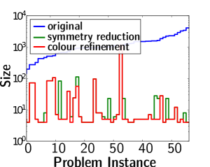
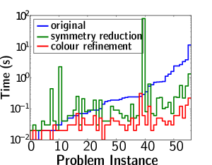
(a)	(b)
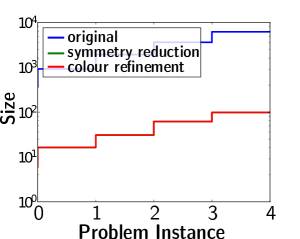
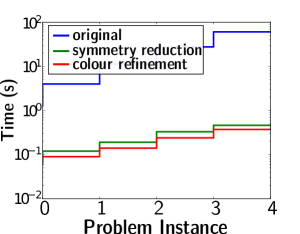
(c)	(d)

Figure 8.1: Computational results on the different linear programs (x-axis). (a) The dimension (number of variables and constraints in log-scale) of the linear programs used for the evaluation. (b) The running times in (log-scaled) seconds (including the time for reduction) for solving the linear programs. Note that for clarity, the values in (a,b) are sorted according to the baseline independently for each figure. We refer the reader to the table in the appendix for the exact numbers. (c,d) Same figures for computing the value functions of the grid Markov decision processes.

The linear programs chosen for the evaluation are relaxed versions of the integer programs available at Francois Margot’s website http://wpweb2.tepper.cmu.edu/fmargot/lpsym.html. They encode combinatorial optimisation problems with applications in coding theory, statistical design and graph theory such as computing maximum cardinality binary error correcting codes, edge colourings, minimum dominating sets in Hamming graphs, and Steiner-triple systems.

The results are summarised in Fig. 8.1(a,b). One can clearly see that colour refinement reduces the dimension of the linear programs at least as much as the symmetry reduction, in many cases — as expected — even more. Looking at the running times, this reduction also results in faster total computations, often an order of magnitude faster. Overall, solving all linear programs took 38 seconds without dimension reduction. Using the symmetry to reduce the dimensions, running all experiments actually increased to 89 seconds, whereas using colour refinement it only took 2 seconds. Indeed, the higher running time when using the symmetry reduction is due to few instances only but also illustrates the benefit of running a guaranteed quasilinear method such as colour refinement for reducing the dimension of linear programs.

Next, we considered the computation of the value function of a Markov Decision Problem modelling decision making in situations where outcomes of actions are partly random. As shown in e.g. [18], the LP is $\operatorname{max}\nolimits_{x}\ 1^{{\textsf{t}}}x,\ \ \text{s.t.}\ \ x_{i}\leq x_{i}^{k}+\gamma\sum\nolimits_{j}p_{ij}^{k}x_{j}\;,$ where $x_{i}$ is the value of state $i$, $c_{i}^{k}$ is the reward that the agent receives when carrying out action $k$ in $i$, and $p_{ij}^{k}$ is the probability of transferring from state $i$ to state $j$ by the action $k$. The MDP instance that we used is the well-known Gridworld, see e.g. [26]. Here, an agent navigates within a grid of $n\times n$ states. Every state has an associated reward $R(s)$. Typically there is one or several states with high rewards, considered the goals, whereas the other states have zero or negative associated rewards. We induced symmetries by putting a goal in every corner of the grid. The results for different grid sizes $n$ are summarised in Fig. 8.1(c,d) and confirm our previous results. Indeed, as expected, colour refinement and automorphisms result in the same partitions but colour refinement is faster.

Finally, triggered by [20], we considered MAP inference in Markov logic networks (MLNs) [24] via the standard LP relaxation for MAP of the induced graphical model, see e.g. [11]. Specifically, we used Richardson and Domingos’ smoker-friends MLN encoding that friends have similar smoking habits. The so-called Frucht (among $12$ people) and McKay (among $8$ people) graphs were used to encode the social network, i.e., who are friends. The induced LPs were of sizes $1710$ resp. $729$. Solving them took $0.35$ resp. $0.05$ seconds. Using symmetry reduction, the sizes reduced to $1590$ resp. $247$. Reducing and solving them took $0.34$ resp $0.02$ seconds. Colour refinement, however, reduced the sizes to $46$ resp $114$. Reducing and solving the corresponding LPs took $0.02$ seconds in both cases.

9 Conclusions

We develop a theory of fractional automorphisms and equitable partitions of matrices and show how it can be used to reduce the dimension of linear programs. The main point is that there is no need to compute full symmetries (that is, automorphisms) to do a symmetry reduction for linear programs, an equitable partition will do, and that colour refinement can compute the coarsest equitable partition very efficiently. We demonstrate experimentally that the gain of our method can be significant, also in comparison with other symmetry reduction methods.

In particular, we benefit from the fact that the colour refinement algorithm on which we rely is very efficient, running in quasilinear time. For really large scale applications, however, it would be desirable to implement the algorithm in a distributed fashion. Towards this end, in [16] we viewed graph isomorphism as a convex optimisation problem and showed that colour refinement can be viewed as a variant of the Franke-Wolfe convex optimisation algorithm. We also gave an algorithm computing the coarsest equitable partition by a variant of the power iteration algorithm for computing eigenvalues.

Our method works well if colour refinement has few colour classes. A key to understanding when this happens might be Atserias and Maneva’s [2] notion of local linear programs. In particular, for local linear programs we may have a substantial reduction for higher levels of the Sherali-Adams hierarchy.

Another interesting open question is whether there exist “approximate versions” of colour refinement that can be used to solve (certain) linear programs approximately and can be implemented even more efficiently.

Appendix A Experimental Results

The following table shows the results of our first series of experiments with Margot’s benchmark (see http://wpweb2.tepper.cmu.edu/fmargot/lpsym.html) in some more detail. The filenames refer to Margot’s benchmark. We run three different solvers: Columns marked “N” refer to the original LP without any reduction. Columns marked “Sr” refer to the LP reduced by symmetry reduction, and columns marked “Cr” refer to the LP reduced by colour refinement. We list the total time for solving the the LPs, including the time for the reduction, the number of variables, and the number of constraints.

	Solution time			Variables			Constraints
Filename	N	Sr	Cr	N	Sr	Cr	N	Sr	Cr
O4_35.lp	0.23	0.03	0.02	280	1	1	840	5	4
bibd1152.lp	0.71	0.21	0.04	462	1	1	1034	4	4
bibd1154.lp	0.72	0.22	0.04	462	1	1	1034	4	4
bibd1331.lp	0.22	0.05	0.01	286	1	1	728	4	4
bibd1341.lp	2.36	0.22	0.05	715	1	1	1586	4	4
bibd1342.lp	2.36	0.23	0.05	715	1	1	1586	4	4
bibd1531.lp	0.74	0.09	0.03	455	1	1	1120	4	4
bibd738.lp	0.0	0.0	0.01	35	1	1	112	4	4
bibd933.lp	0.01	0.01	0.0	84	1	1	240	4	4
ca36243.lp	0.01	0.02	0.01	64	1	1	368	3	3
ca57245.lp	0.05	0.08	0.02	128	1	1	816	3	3
ca77247.lp	0.06	0.07	0.02	128	1	1	816	3	3
clique9.lp	0.21	0.04	0.02	288	1	1	720	5	4
cod105.lp	11.18	1.31	0.21	1024	1	1	3072	3	3
cod105r.lp	2.62	0.55	0.11	638	3	3	1914	9	9
cod83.lp	0.19	0.06	0.02	256	1	1	768	3	3
cod83r.lp	0.16	0.03	0.02	219	6	6	657	18	18
cod93.lp	1.28	0.15	0.03	512	1	1	1536	3	3
cod93r.lp	1.1	0.1	0.02	466	7	7	1398	21	21
codbt06.lp	3.28	0.21	0.04	729	1	1	2187	3	3
codbt24.lp	0.34	0.07	0.02	324	1	1	972	3	3
cov1053.lp	0.18	0.11	0.04	252	1	1	679	5	5
cov1054.lp	0.23	0.13	0.04	252	1	1	889	6	6
cov1054sb.lp	0.24	0.3	0.3	252	252	252	898	898	898
cov1075.lp	0.05	0.24	0.06	120	1	1	877	7	7
cov1076.lp	0.06	0.2	0.04	120	1	1	835	7	7
cov1174.lp	0.52	0.61	0.11	330	1	1	1221	6	6
cov954.lp	0.04	0.05	0.02	126	1	1	507	6	6
flosn52.lp	0.17	0.03	0.02	234	4	1	780	19	4
flosn60.lp	0.23	0.04	0.01	270	4	1	900	19	4
flosn84.lp	0.58	0.06	0.01	378	4	1	1260	19	4
jgt18.lp	0.02	0.01	0.01	132	19	19	402	87	87
jgt30.lp	0.13	0.03	0.0	228	20	10	690	92	46
mered.lp	1.57	0.06	0.02	560	4	1	1680	19	4
oa25332.lp	0.18	0.08	0.03	243	1	1	1026	4	4
oa25342.lp	0.23	0.05	0.02	243	1	1	1296	4	4
oa26332.lp	3.74	0.53	0.12	729	1	1	2538	4	4
oa36243.lp	0.01	0.03	0.02	64	1	1	608	4	4
oa56243.lp	0.01	0.03	0.01	64	1	1	608	4	4
oa57245.lp	0.09	0.18	0.04	128	1	1	1376	4	4
oa66234.lp	0.01	0.02	0.01	64	16	16	212	56	56
oa67233.lp	0.03	0.03	0.01	128	20	20	384	64	64
oa68233.lp	0.18	0.08	0.03	256	24	24	698	72	72
oa76234.lp	0.0	0.01	0.0	64	16	16	212	56	56
oa77233.lp	0.03	0.03	0.01	128	20	20	384	64	64
oa77247.lp	0.08	0.18	0.05	128	1	1	1376	4	4
of5_14_7.lp	0.06	0.02	0.01	175	15	1	490	68	4
of7_18_9.lp	0.7	0.05	0.02	441	5	1	1134	23	4
ofsub9.lp	0.08	0.02	0.01	203	7	7	527	32	32
pa36243.lp	0.0	0.02	0.01	64	1	1	368	3	3
pa57245.lp	0.07	0.08	0.02	128	1	1	816	3	3
pa77247.lp	0.08	0.08	0.02	128	1	1	816	3	3
sts135.lp	0.28	79.18	0.05	135	1	1	3285	7	3
sts27.lp	0.0	0.01	0.0	27	1	1	171	3	3
sts45.lp	0.01	0.43	0.0	45	1	1	420	7	3
sts63.lp	0.02	2.22	0.01	63	1	1	777	5	3
sts81.lp	0.04	0.05	0.02	81	1	1	1242	3	3

References

- [1] B. Ahmadi, K. Kersting, M. Mladenov, and S. Natarajan. Exploiting symmetries for scaling loopy belief propagation and relational training. Machine Learning Journal, 92:91–132, 2013.
- [2] A. Atserias and E. Maneva. Sherali–Adams relaxations and indistinguishability in counting logics. SIAM Journal on Computing, 42(1):112–137, 2013.
- [3] C. Berkholz, P. Bonsma, and M. Grohe. Tight lower and upper bounds for the complexity of canonical colour refinement. In Proceedings of the 21st Annual European Symposium on Algorithms, 2013. To appear.
- [4] R. Bödi, T. Grundhöfer, and K. Herr. Symmetries of linear programs. Note di Matematica, 30(1):129–132, 2010.
- [5] Richard Bödi, Katrin Herr, and Michael Joswig. Algorithms for highly symmetric linear and integer programs. Mathematical Programming, 137(1-2):65–90, 2013.
- [6] Stephen Boyd, Persi Diaconis, and Lin Xiao. Fastest mixing markov chain on a graph. SIAM REVIEW, 46:667–689, 2003.
- [7] David Bremner, Mathieu Dutour Sikiric, and Achill Schürmann. Polyhedral representation conversion up to symmetries. In CRM proceedings, volume 48, pages 45–72. American Mathematical Society, Providence, 2009.
- [8] H.H. Bui, T.N. Huynh, and S. Riedel. Automorphism groups of graphical models and lifted variational inference. In Proc. of the 29th Conference on Uncertainty in Artificial Intelligence (UAI-2013), 2013. (To appear).
- [9] A. Cardon and M. Crochemore. Partitioning a graph in . Theoretical Computer Science, 19(1):85 – 98, 1982.
- [10] Karin Gatermann and Pablo A. Parrilo. Symmetry groups, semidefinite programs, and sums of squares. Journal of Pure and Applied Algebra, 192(1–3):95 – 128, 2004.
- [11] A. Globerson and T. Jaakkola. Fixing max-product: Convergent message passing algorithms for map LP-relaxations. In Proc. of the 21st Annual Conf. on Neural Inf. Processing Systems (NIPS), 2007.
- [12] C.D. Godsil. Compact graphs and equitable partitions. Linear Algebra and its Applications, 255:259–266, 1997.
- [13] J.E. Hopcroft. An n log n algorithm for minimizing states in a finite automaton. In Z. Kohavi and A. Paz, editors, Theory of Machines and Computations, pages 189–196. Academic Press, 1971.
- [14] Hadi Katebi, Karem A. Sakallah, and Igor L. Markov. Graph symmetry detection and canonical labeling: Differences and synergies. In Andrei Voronkov, editor, Turing-100, volume 10 of EPiC Series, pages 181–195. EasyChair, 2012.
- [15] K. Kersting, B. Ahmadi, and S. Natarajan. Counting Belief Propagation. In Proc. of the 25th Conf. on Uncertainty in Artificial Intelligence (UAI–09), 2009.
- [16] K. Kersting, M. Mladenov, R. Garnet, and M. Grohe. Power iterated color refinement. In Proceedings of the 28th AAAI Conference on Artificial Intelligence, 2014. To appear.
- [17] Leo Liberti. Reformulations in mathematical programming: automatic symmetry detection and exploitation. Mathematical Programming, 131(1-2):273–304, 2012.
- [18] M.L. Littman, T.L. Dean, and L. Pack Kaelbling. On the complexity of solving markov decision problems. In Proc. of the 11th International Conference on Uncertainty in Artificial Intelligence (UAI-95), pages 394–402, 1995.
- [19] François Margot. Symmetry in integer linear programming. In Michael Jünger, Thomas M. Liebling, Denis Naddef, George L. Nemhauser, William R. Pulleyblank, Gerhard Reinelt, Giovanni Rinaldi, and Laurence A. Wolsey, editors, 50 Years of Integer Programming 1958-2008, pages 647–686. Springer Berlin Heidelberg, 2010.
- [20] M. Mladenov, B. Ahmadi, and K. Kersting. Lifted linear programming. In 15th Int. Conf. on Artificial Intelligence and Statistics (AISTATS 2012), pages 788–797, 2012. Volume 22 of JMLR: W&CP 22.
- [21] R. Paige and R.E. Tarjan. Three partition refinement algorithms. SIAM Journal on Computing, 16(6):973–989, 1987.
- [22] J.-F. Puget. Automatic detection of variable and value symmetries. In Peter Beek, editor, Principles and Practice of Constraint Programming - CP 2005, volume 3709 of Lecture Notes in Computer Science, pages 475–489. Springer Berlin Heidelberg, 2005.
- [23] M.V. Ramana, E.R. Scheinerman, and D. Ullman. Fractional isomorphism of graphs. Discrete Mathematics, 132:247–265, 1994.
- [24] M. Richardson and P. Domingos. Markov Logic Networks. Machine Learning, 62:107–136, 2006.
- [25] P. Singla and P. Domingos. Lifted First-Order Belief Propagation. In Proc. of the 23rd AAAI Conf. on Artificial Intelligence (AAAI-08), pages 1094–1099, Chicago, IL, USA, July 13-17 2008.
- [26] R.S. Sutton and A.G. Barto. Reinforcement Learning: An Introduction. The MIT Press, 1998.
- [27] G. Tinhofer. A note on compact graphs. Discrete Applied Mathematics, 30:253–264, 1991.