An asymptotic theory for waves guided by diffraction gratings or along microstructured surfaces

Abstract

Plasmonics, Homogenization, Rayleigh-Bloch waves

An effective surface equation, that encapsulates the detail of a microstructure, is developed to model microstructured surfaces. The equations deduced accurately reproduce a key feature of surface wave phenomena, created by periodic geometry, that are commonly called Rayleigh-Bloch waves, but which also go under other names such as Spoof Surface Plasmon Polaritons in photonics. Several illustrative examples are considered and it is shown that the theory extends to similar waves that propagate along gratings. Line source excitation is considered and an implicit long-scale wavelength is identified and compared to full numerical simulations. We also investigate non-periodic situations where a long-scale geometric variation in the structure is introduced and show that localised defect states emerge which the asymptotic theory explains.

1 Introduction

It has been known for many years that surface waves, that is, waves propagating along a surface, and exponentially decaying in amplitude perpendicular to the surface, are created by geometric periodic corrugations, or perturbations, to the surface Barlow & Karbowiak (1954); Hurd (1954); Brekhovskikh (1959) in situations where a surface wave would otherwise not exist. Such surface waves also exist for diffraction gratings and for trapped modes in waveguides; these are all very similar problems mathematically McIver et al. (1998); Porter & Evans (1999) and differ just in their setting. These surface waves have been discovered in many different areas of wave mechanics and go under names such as edge waves Evans & Linton (1993) for water waves localised to periodic coastlines, spoof surface plasmon polaritons, SPPs, Pendry et al. (2004); Fernandez-Dominguez et al. (2011) in modern applications of plasmonics, array guided surface waves Sengupta (1959) in Yagi-Uda antenna theory, Rayleigh-Bloch surface waves Wilcox (1984); Porter & Evans (1999) for diffraction gratings amongst other areas: We will call them Rayleigh-Bloch waves as surface waves are typically called Rayleigh waves and Bloch waves arise due to periodicity. They can also be identified in lattice defect arrays, in discrete settings Joseph & Craster (2013), and are ubiquitous across wave mechanics, it is important to clearly delineate them from surface waves, such as Rayleigh waves, that are present in the absence of periodic geometric features and which arise due to material mismatch or from wave mode coupling at the surface.

Naturally, as these are eigenfunctions of a diffraction problem and have implications for the uniqueness of solutions they have been the subject of numerous existence studies Wilcox (1984); Bonnet-Bendhia & Starling (1994); Linton & McIver (2002) with the conclusion that they are a generic property of periodic surfaces and gratings that have Neumann boundary conditions: The non-existence for Dirichlet cases is shown in Wilcox (1984).

As well as being ubiquitous in wave mechanics, Rayleigh-Bloch waves are important in applications; their dispersion characteristics can be carefully tuned by altering only the geometry as in SPPs Fernandez-Dominguez et al. (2011), or are important through the coupling of incident waves into Rayleigh-Bloch waves causing near resonant effects for finite arrays as in water waves Maniar & Newman (1997). These effects, and in particular the possibility to tune or de-tune them, rely upon being able to simulate and determine dispersion characteristics; there is advantage in being able to represent and model them using an effective medium approach that replaces the microstructure.

The classical route to replace a microstructured medium with an effective continuum representation is homogenization theory, and for bulk media this is detailed in many monographs, for instance Sanchez-Palencia (1980); Bakhvalov & Panasenko (1989); Bensoussan et al. (1978); Panasenko (2005) and essentially relies upon the wavelength being much larger than the microstructure which is usually assumed to be perfectly periodic: The theory has been very versatile and has been widely applied. Naturally there were extensions of this theory to surfaces, notably by Nevard & Keller (1997), again with the wavelength limitation, unfortunately this long-wave low frequency limit is not particularly useful at the high frequencies used in applications such as photonics Joannopoulos et al. (2008) and plasmonics Maier (2007); Enoch & Bonod (2012): This motivated the development of high frequency homogenization (HFH) in Craster et al. (2010a). HFH breaks free of the low frequency long-wave limitation and, for bulk media, creates effective long-scale equations that encapsulate the microstructural behaviour, which can be upon the same scale as the wavelength, through integrated quantities that are no longer simple averages. The methodology relies upon there being some basic underlying periodic structure so that Bloch waves, and standing wave frequencies, encapsulate the multiple scattering between elements of the microstructure on the short scale, and this is then modulated by a long scale function that satisfies an anisotropic frequency dependent partial differential equation; the technique has been successfully applied to acoustics/ electromagnetics Craster et al. (2011); Antonakakis et al. (2013), elastic plates that support bending waves Antonakakis & Craster (2012), frames Nolde et al. (2011) and to discrete media Craster et al. (2010b). The advantage of having an effective equation for a microstructured bulk medium or surface is that one need no longer model the detail of each individual scatterer, as they are subsumed into a parameter on the long-scale, and attention can then be given to the overall physics of the structure and one can identify, or design for, novel physics.

The HFH theory of Craster et al. (2010a) is not alone: There is considerable interest in creating effective continuum models of microstructured media, in various related fields, that break free from the conventional low frequency homogenisation limitations. This desire has created a suite of extended homogenization theories originating in applied analysis, for periodic media, called Bloch homogenisation Conca et al. (1995); Allaire & Piatnitski (2005); Birman & Suslina (2006); Hoefer & Weinstein (2011). There is also a flourishing literature on developing homogenized elastic media, with frequency dependent effective parameters, also based upon periodic media as in Nemat-Nasser et al. (2011). Those approaches notwithstanding, our aim here is to extend the HFH theory to microstructured surfaces and obtain frequency dependent effective surface conditions that capture the main features of the surface waves that exist.

Our aim herein is to generate a surface HFH theory for structured surfaces in the context of perfect surfaces, importantly one can modify the theory, as done for bulk waves in Craster et al. (2011); Antonakakis & Craster (2012); Makwana & Craster (2012), to pull out defect states associated with non-periodic variation. It is also important to note that the HFH theory has a deep connection with the high frequency long wavelength near cutoff theory of waveguides Craster et al. (2013) and the defect states are related to localisation by deformed waveguides Gridin et al. (2004); Kaplunov et al. (2005); Gridin et al. (2005). We also naturally extend the HFH theory to diffraction gratings. In section 2 the theory is created culminating in the effective equation that encapsulates the surface behaviour. Illustrative examples, in section 3, then show the efficacy of the methodology versus the dispersion relations found numerically. An interesting practical situation is where some geometric variation occurs, then one expects the possibility of trapped modes along the structure occuring at a set of discrete frequencies, and we consider a comb-like structure where the teeth have varying length in section 4; the asymptotic theory is compared to full numerical simulations. Finally, concluding comments and remarks are drawn together in section 5.

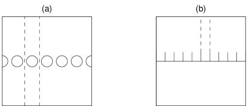
Figure 1: A diffraction grating of cylinders shown in (a), and (b) shows a periodic “comb” surface that supports spoof surface plasmons. Both panels have the elementary strip shown as the dashed lines.

2 General theory

For perfect infinite linear arrays, diffraction gratings or surface structures arranged periodically, one focuses attention on a single elementary strip of material that then repeats (see Fig. 1 for illustrative cases); quasi-periodic Floquet-Bloch boundary conditions describe the phase-shift across the strip as a wave moves from strip to strip through the material. Rayleigh-Bloch waves are special as they consist of waves that also decay exponentially in the perpendicular direction away from the array. Dispersion relations then relate the Floquet-Bloch wavenumber, the phase-shift, to frequency. Although the problem is truly two-dimensional, the assumption of exponential decay in the perpendicular renders it quasi-one dimensional with the wavenumber remaining scalar; this contrasts with the theory of Bloch waves in photonic crystals Joannopoulos et al. (2008) where a vector wavenumber and the Brillouin zone are more natural descriptions.

We shall approach the problem tangentially and generate an asymptotic theory, importantly we take Neumann boundary conditions on the lattice or surface; physically, this can be considered as TE (transverse electric) polarization for a perfectly conducting surface which is a good model for microwaves Petit (1980).

A time harmonic dependence of propagation $\exp(-i\omega t)$, with frequency $\omega$, is assumed throughout, and henceforth suppressed, and after non-dimensionalisation one arrives at

$$\nabla^{2}_{{\bf x}}u({\bf x})+\Omega^{2}u({\bf x})=0,\qquad\text{with}\quad\Omega=\frac{\omega l}{c},$$ (1)

where $l$ is the lengthscale of the micro-scale and $c$ is the wavespeed, as the governing equation of interest. We consider the half-space $-\infty<x_{1}<\infty$, $0<x_{2}<\infty$, and for the grating extend to $-\infty$ in $x_{2}$. In (1), $\Omega$ is the non-dimensional frequency and $u$ is the out-of-plane displacement in elasticity or the $H_{3}$ component of the magnetic field in TE polarisation.

The two-scale nature of the problem is incorporated using small and large length scales to define two new independent coordinates namely $X=x_{1}/L$, and $(\xi_{1},\xi_{2})=(x_{1},x_{2})/l$. The implicit assumption is that there is a small scale, characterized by $l$, and a long scale characterized by $L$ where $\epsilon=l/L\ll 1$. As the structure is quasi-one dimensional, with the mismatch in the scales being just along the structure, we only introduce a single long-scaled variable in $X$; we do not introduce a long-scale $Y$ in the $x_{2}$ direction as it is redundant.

Under this rescaling, equation (1) then becomes,

$$\left[\frac{\partial^{2}}{\partial\xi_{1}^{2}}+2\epsilon\frac{\partial^{2}}{\partial\xi_{1}\partial X}+\epsilon^{2}\frac{\partial^{2}}{\partial X^{2}}+\frac{\partial^{2}}{\partial\xi_{2}^{2}}+\Omega^{2}\right]u(X,\xi_{1},\xi_{2})=0.$$ (2)

Standing waves, that exponentially decay perpendicular to the surface/ grating, can occur when there are periodic (or anti-periodic) boundary conditions across the elementary strip (in the ${\bm{\xi}}$ coordinates) and these standing waves encode the local information about the multiple scattering that occurs by the neighbouring strips. The asymptotic technique we create is a perturbation about these standing wave solutions, as these are associated with periodic and anti-periodic boundary conditions, which are respectively in-phase and out-of-phase waves across the strip, the conditions on the short-scale ${\bm{\xi}}$ on the edges of the strip, $\partial S_{1}$, are known:

$$u|_{\xi_{1}=1}=\pm u|_{\xi_{1}=-1}\quad\text{and}\quad u_{,\xi_{1}}|_{\xi_{1}=1}=\pm u_{,\xi_{1}}|_{\xi_{1}=-1},$$ (3)

where $u_{,\xi_{i}}$ denotes differentiation of $u$ with respect to variable $\xi_{i}$ and with the $+,-$ for periodic or anti-periodic cases respectively. There is therefore a local solution on the small scale that incorporates the multiple scattering of a periodic medium and that will then be modulated by a long-scale function that satisfies a differential equation. Typically, the periodic case corresponds to long-waves relative to the structure - this case is not particularly interesting and is captured by conventional low-frequency homogenisation. We therefore concentrate upon the anti-periodic case.

We pose an ansatz for the field and the frequency,

$$u(X,{\bm{\xi}})=u_{0}(X,{\bm{\xi}})+\epsilon u_{1}(X,{\bm{\xi}})+\epsilon^{2}u_{2}(X,{\bm{\xi}})+\ldots,$$

$$\Omega^{2}=\Omega_{0}^{2}+\epsilon\Omega_{1}^{2}+\epsilon^{2}\Omega_{2}^{2}+\ldots$$ (4)

The $u_{i}(X,{\bm{\xi}})$’s adopt the boundary conditions (3) on the short-scale, with the minus sign for anti-periodicity, on the edge of the strip. An ordered hierarchy of equations emerge in powers of $\epsilon$, and are treated in turn

$$u_{0,\xi_{i}\xi_{i}}+\Omega_{0}^{2}u_{0}=0,$$ (5)

$$u_{1,\xi_{i}\xi_{i}}+\Omega_{0}^{2}u_{1}=-2u_{0,\xi_{1}X}-\Omega_{1}^{2}u_{0},$$ (6)

$$u_{2,\xi_{i}\xi_{i}}+\Omega_{0}^{2}u_{2}=-u_{0,XX}-2u_{1,\xi_{1}X}-\Omega_{1}^{2}u_{1}-\Omega_{2}^{2}u_{0}.$$ (7)

The leading order equation (5) is independent of the long-scale $X$ and is a standing wave on the elementary strip existing at a specific eigenfrequency $\Omega_{0}$ and has associated eigenmode $U_{0}({\bm{\xi}};\Omega_{0})$, modulated by a long-scale function $f_{0}(X)$ and so we expect to get an ordinary differential equation (ODE) for $f_{0}$ as an effective boundary, or interface, condition characterising the grating when viewed from afar: To leading order

$$u_{0}(X,{\bm{\xi}})=f_{0}(X)U_{0}({\bm{\xi}};\Omega_{0}).$$ (8)

The entire aim is to arrive at an ODE for $f_{0}$ posed entirely upon the long-scale, but with the microscale incorporated through coefficients that are integrated, not necessarily averaged, quantities.

Before we continue to next order, equation (6), we define the Neumann boundary conditions on the inclusions, or the micro-structured surface, $\partial S_{2}$, as

$$\frac{\partial u}{\partial{\bf n}}=u_{,x_{i}}n_{i}|_{\partial S_{2}}=0,$$ (9)

using Einstein’s notation for summation over repeated indices, and where ${\bf n}$ is the outward pointing normal, which in terms of the two-scales and $u_{i}(X,{\bm{\xi}})$ become

$$U_{0,\xi_{i}}n_{i}=0,\quad U_{0}f_{0,X}n_{1}+u_{1,\xi_{i}}n_{i}=0,\quad u_{1,X}n_{1}+u_{2,\xi_{i}}n_{i}=0.$$ (10)

The leading order eigenfunction $U_{0}({\bm{\xi}};\Omega_{0})$ must satisfy the first of these conditions and it is relatively straightforward to extract this either numerically, as we do later, or using semi-analytic methods such as the residue calculus technique Hurd (1954).

Moving to the first order equation (6) we invoke a solvability condition by integrating over the elementary strip, which is on the short-scale ${\bm{\xi}}$, the product of equation (6) and $U_{0}$ minus the product of equation (5) and $u_{1}/f_{0}({X})$: The result is that the eigenvalue $\Omega_{1}$ is identically zero.

We then solve for $u_{1}=f_{0,X}U_{1}({\bm{\xi}})$, so $U_{1}$ satisfies

$$\nabla_{{\bm{\xi}}}^{2}U_{1}+\Omega_{0}^{2}U_{1}=-2U_{0,\xi_{1}}$$ (11)

subject to the boundary condition

$${\bf n}\cdot\nabla_{{\bm{\xi}}}U_{1}=-U_{0}n_{1},$$ (12)

on $\partial S_{2}$. Again solutions can be found numerically or using semi-analytic methods.

Going to second-order, a similar solvability condition to that used at first order is applied using equation (7); after some algebra we obtain the desired ordinary differential equation for $f_{0}$

$$Tf_{0,XX}+\Omega_{2}^{2}f_{0}=0$$ (13)

posed entirely on the long-scale $X$. The coefficient $T$ is constructed from integrals over the elementary strip in ${{\bm{\xi}}}$ and is ultimately independent of ${\bm{\xi}}$. The formula for $T$ is

$$T{\int\int_{S}U_{0}^{2}dS}=\int\int_{S}(U_{0}^{2}+2U_{1,\xi_{1}}U_{0})dS-\int_{\partial S_{2}}U_{1}U_{0}n_{1}ds,$$ (14)

which using Green’s Theorem, with vector field ${\bf F}=(U_{1}U_{0},0)$, simplifies to,

$$T{\int\int_{S}U_{0}^{2}dS}=\int\int_{S}(U_{0}^{2}+U_{1,\xi_{1}}U_{0}-U_{0,\xi_{1}}U_{1})dS.$$ (15)

For an infinite perfect grating, the Bloch grating, one sets $f_{0}(X)=\exp(i[\pi/2-\kappa]X/\epsilon)$ and equation (13) simplifies to $\Omega_{2}^{2}=[\pi/2-\kappa]^{2}T/\epsilon^{2}$ and from (4) the asymptotic dispersion relation relating frequency, $\Omega$, to Bloch wavenumber, $\kappa$, is

$$\Omega\sim\Omega_{0}+\frac{T}{2\Omega_{0}}[\pi/2-\kappa]^{2}.$$ (16)

In (16) $T$ is invariably negative, c.f Table 1 for some illustrative values, as is $\Omega_{2}^{2}$, the latter should not be confused with having negative frequencies as it is just a frequency perturbation. Therefore, if the surface or grating supports Rayleigh-Bloch waves then they are represented as an effective string or membrane equation (13) where the effective stiffness (or effective inverse of permittivity in the context of photonics) of the string is $T$; all the microstructural and geometrical information is contained in this asymptotic result and one can then extend it to be used for finite arrays or for slightly non-periodic arrays, or forced problems etc, but our aim here is to now demonstrate that this theory is well-founded.

Figure 2: The dispersion branches for the comb-like structure. Solid-lines are from (21), and the light-line $\Omega=\kappa$ is the dotted line. Panels (a), (b), (c) and (d) are for $a=1$, $3$, $5$ and $7$ respectively. Asymptotics from HFH (16), with $T$ given in Table 1 for $a=7$ (d), are shown as dashed curves.

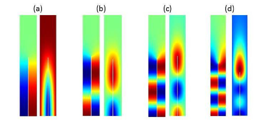
Figure 3: The eigenfunctions $U_{0}$, and $U_{1}$ shown for the comb-like structure with $a=7$ c.f. Fig. 2(d). These are for the standing wave frequencies $\Omega_{0}$ in Table 1 with (a)-(d) for ascending $\Omega_{0}$. In each panel $U_{0}$ is shown on the left and $U_{1}$ on the right.

$T$	$\Omega_{0}$
$-0.006485497624108$	$0.210161050669707$
$-0.067470169867289$	$0.629209426388598$
$-0.280897588912595$	$1.043323585456635$
$-2.350025233704123$	$1.440535862845912$

Table 1: The four standing wave frequencies for the comb-like structure with $a=7$, c.f. Fig. 2(d), together with associated values for $T$.

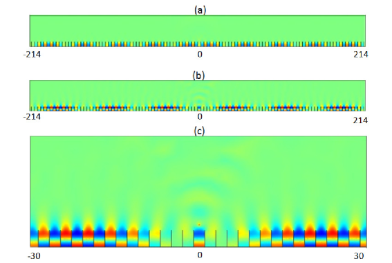
Figure 4: Plots of real$(u)$ from finite element simulations for a comb grating with $a=3$ c.f. Fig. 2(b): (a) Fields generated by a line source with $\Omega=0.4509$ ($\Omega_{0}=0.45127$); (b) Fields generated by a line source with $\Omega=1.3138$ ($\Omega_{0}=1.31510$);(c) Detail of real $(u)$ at $\Omega=1.3138$.

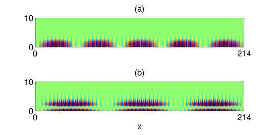
Figure 5: Plots of real$(u)$ from HFH for a comb with $a=3$, c.f. Fig. 4, generated by a line source at (a) $\Omega=0.4509$ and (b) $\Omega=1.3138$ respectively.

2.1 The classical long wave zero frequency limit

The current theory simplifies dramatically in the classical long wave, low frequency, limit where $\Omega^{2}\sim O(\epsilon^{2})$, this is a periodic case on the short-scale: $U_{0}$ becomes uniform, and without loss of generality, is set to be unity over the elementary strip. The final equation is again (13) where $T$ simplifies to

$$T\int\int_{S}dS=\int\int_{S}dS+\int\int_{S}U_{1,\xi_{1}}dS.\quad$$ (17)

$U_{1_{i}}$ satisfies the Laplacian $U_{1,\xi_{i}\xi_{i}}=0$ and $U_{1}$ has boundary conditions $U_{1,\xi_{i}}n_{i}=-n_{1}$ on $\partial S_{2}$. Rearranging equation (17) yields, using a rectangular strip of height $y^{*}$ for $S$,

$$T=1+\frac{\int\int_{S}U_{1,\xi_{i}}dS}{\lim\limits_{y^{*}\to+\infty}\int_{0}^{y^{*}}2dy}\rightarrow 1,$$ (18)

from which $\Omega=\kappa$ and thus the light-line of unit slope emerging from the origin arises asymptotically.

Figure 6: The dispersion branches, for the symmetric mode, ($\Omega=\kappa$ as dotted line) are shown in panel (a) for cylinders with radii of $0.7$ (dashed bold), $0.5$ (bold) and $0.4$ (solid). The corresponding asymptotic curves, from (16), are shown as dashed lines. Panel (b) shows the standing wave eigensolution $U_{0}$ for $r=0.5$.

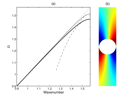
Figure 7: The dispersion branches, for the antisymmetric mode, ($\Omega=\kappa$ as dotted line) are shown in panel (a) for cylinders with radii of $0.95$ (solid line) and $0.99$ (bold solid line). The asymptotics are shown as dashed lines. In panel (b) the antisymmetric eigensolution $U_{0}$ is shown for $r=0.95$.

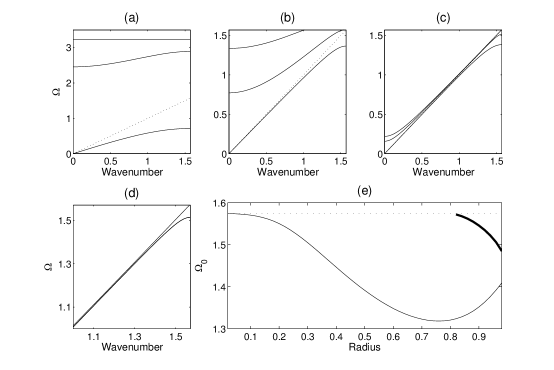
Figure 8: The dispersion curves for cylinders placed in a rectangular array are shown for Bloch waves in the $x_{1}$ direction. The lowest three dispersion branches, as solid lines, and $\Omega=\kappa$ as dotted, are shown in (a), (b) and (c) for rectangle heights of $2$, $6$ and $30$ respectively where the cylinder radius is $0.95$. Panel (d) shows the dispersion curves for a cell of height $30$, in solid the second modes for the respective radii of $0.4$ and $0.95$ and the lightline in dashed. Panel (e) shows the variation of standing wave frequencies for the symmetric (solid) and asymmetric (bold) modes versus cylinder radius for the infinite strip.

Figure 9: Plots of real $(u)$ for a diffraction grating consisting of cylinders of radius $r=0.95$: (a) Asymmetric fields generated by a dipole source for $\Omega=1.508$ ($\Omega_{0}=1.51445$); (b) Detail close to the dipole source showing the micro-scale asymmetry; (c) Detail of the real part (upper panel) and absolute value (lower panel) of the asymmetric $u$ at $\Omega=1.508$; (d) Symmetric fields generated by a line source at frequency $\Omega=1.38$ ($\Omega_{0}=1.38407$).

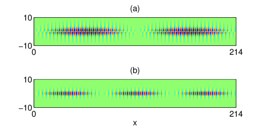
Figure 10: Plots of real $(u)$ from HFH for a cylinder of radius $r=0.95$, c.f. Fig. 9, generated by a line source at (a) $\Omega=1.508$ and (b) $\Omega=1.38$ respectively

2.2 A dynamic characteristic length scale

As we will see later, in section 3, equation (16) is an excellent asymptotic approximation for the dispersion diagrams of such gratings which verifies the validity of HFH. Ultimately one wishes to homogenize a periodic, or nearly periodic, surface and this is achieved with equation (13) transformed back in the original coordinates together with the replacement of $\Omega_{2}$ using the asymptotic expansion in equation (4). The effective medium equation resulting from such operations is,

$$Tf_{0,xx}+(\Omega^{2}-\Omega_{0}^{2})f_{0}=0.$$ (19)

The solutions of equation (19) are harmonic with argument $\sqrt{(\Omega^{2}-\Omega_{0}^{2})/{T}}$ provided $\Omega<\Omega_{0}$ and $T<0$. It is now clear that if the excitation frequency is slightly away from the standing wave frequency there will be an oscillation with wavelength $\lambda=2\pi\sqrt{T/(\Omega^{2}-\Omega_{0}^{2})}$ which will represent a characteristic length scale for such an infinite periodic medium. That length scale not only depends on the excitation and standing wave frequencies but also on the homogenized parameter $T$ that represents dynamically averaged material parameters. Therefore one observes highly oscillatory behaviour with each neighbouring strip out-of-phase but modulated by a long-scale oscillation of wavelength $\lambda/2$ reminiscent of a beat frequency but induced by the microstructure; the $\lambda/2$ arises as one observes both $f_{0}$ and $-f_{0}$.

3 Illustrative examples

We now illustrate the theory using linear arrays of cylinders, split ring resonators (SRR) and a comb-like surface structure as these are exemplars of the situations seen in practice.

3.1 The classical comb

An early example for which Rayleigh-Bloch waves were found explicitly is that of a Neumann comb-like surface consisting of periodic thin plates of finite length, $a$, perpendicular to a flat wall and distant by $2l$ from each other. This was initially studied by Hurd (1954) with later modifications by DeSanto (1972); Evans & Linton (1993); Evans & Porter (2002): It is a canonical example and can be considered as a diffraction grating if extended to the negative half-plane by reflexion symmetry.

We will concentrate upon non-embedded Rayleigh-Bloch waves in $\Omega<\kappa$ and Hurd’s dispersion relation

$$\Omega a/l=(n+1/2)\pi+2\Omega/\pi\ln 2+\chi(\kappa,2\Omega)$$ (20)

where

$$\chi(\kappa,\Omega)=-\sin^{-1}(\Omega/\kappa)+\sum_{n=1}^{\infty}\left(\sin^{-1}(\Omega/n\pi)-\sin^{-1}(\Omega/(\kappa+2n\pi))-\sin^{-1}(\Omega/|\kappa-2n\pi|)\right)$$ (21)

provides a highly accurate approximation; dispersion branches are shown in Fig. 2 using Hurd’s formulae. There exists an even more accurate result from Evans & Linton (1993) which is virtually indistinguishable from that of Hurd, and it is possible, as we also do here, to use finite elements to model the comb numerically, the only detail of note is that the comb teeth have finite width of $0.05$ in the finite element simulations to avoid any numerical issues at the tip of the teeth, and all these methods give coincident results. The dispersion equations (21) come from a Fourier series approach and we also investigate this approach numerically and provide results in Tables 2,3. The parameter $a$ is the length of the tooth, and the curves are locally quadratic near $\pi$ as we expect from (16); clearly the HFH asymptotics provide an excellent representation of the dispersion curves close to the standing wave frequency as illustrated by the dashed curves in Fig. 2. The standing wave frequencies $\Omega_{0}$ and the effective parameter $T$ are given in Table 1 for the case $a=7$. Increasing $a$ corresponds to more dispersion curves appearing and the eigensolutions for $a=7$ are shown in Fig. 3 together with their $U_{1}$ counterparts, and the reason for the increasing number of surface modes is immediately apparent being intimately connected with the number of modes the open waveguide supports. The $U_{0}$ modes decay rapidly as they exit the open waveguide particularly for the lowest standing wave frequencies.

This physical interpretation then motivates a Fourier series approach and using a rescaling of lengths and frequencies, $\hat{\xi}=\xi/2$, $\hat{y}=y/2$, $\hat{a}=a/2$, $\hat{\Omega}=2\Omega$ and $\hat{\kappa}=2\kappa$ gives the geometry investigated by Evans & Linton (1993). The full Rayleigh-Bloch solution for $u$ is obtained as

$$u(\hat{\xi},\hat{y})=\left\{\begin{array}[]{ll}\displaystyle{\sum_{n=0}^{\infty}A_{n}\cos p_{n}\hat{\xi}\cosh\alpha_{n}\hat{y}}&0\leq\hat{y}\leq\hat{a}\\[10.00002pt] \displaystyle{\sum_{n=-\infty}^{\infty}B_{n}{\rm e}^{{\rm i}\kappa_{n}\hat{\xi}}{\rm e}^{-\gamma_{n}(\hat{y}-\hat{a})}}&\hat{y}\geq\hat{a}\end{array}\right.$$ (22)

where $p_{n}=n\pi$, $\alpha_{n}=\sqrt{p_{n}^{2}-\hat{\Omega}^{2}}$, $\kappa_{n}=(2n\pi+\hat{\kappa})$, and $\gamma_{n}=\sqrt{\kappa_{n}^{2}-\hat{\Omega}^{2}}$. The coefficients are determined by imposing continuity of $u$ and $\partial u/\partial\hat{y}$ at $\hat{y}=\hat{a}$, multiplying by $\cos p_{m}\hat{\xi}$ and integrating across the cell width, which allows the $A_{n}$ to be eliminated and leaves a set of linear equations for the $\kappa_{n}B_{n}$ coefficients which are written in matrix notation as

$$\bf{M}\hskip 4.30554pt(\boldmath{\kappa B})=\bf{0}{\rm,}$$ (23)

where ${\bf M}$ is a matrix that can be deduced from Evans & Linton (1993). The dispersion relation is obtained by fixing values of $\hat{\kappa}$ and finding the corresponding values of $\hat{\Omega}$ for which $\det({\bf M})=0$, and then obtaining the eigensolutions for the coefficients $\kappa_{n}B_{n}$. The standing wave eigensolution $u_{0}$ is the case where $\kappa=\pi/2$, $\hat{\kappa}=\pi$, $\Omega=\Omega_{0}$, and some of the rows of $\bf{M}$ exhibit singularites. This then requires modifications and the limiting value of the corresponding equations must then be utilised in place of those of Evans & Linton (1993). Numerically the infinite summations are truncated for some value of $N$ of modes and the infinite summations are replaced by $\sum_{-N}^{N-1}$ and $\sum_{0}^{2N}$. For the standing waves the $A_{n}$ are non-zero only for even values of $n$, and the $B_{n}$ satisfy $B_{n}+B_{-(n+1)}=0$. As a consequence, $u_{0}$ is non-zero on the teeth of the comb for $\hat{y}\leq\hat{a}$, and when repeated in the next strip with a sign change exhibits a discontinuity at $\hat{y}=\hat{a}$. The Fourier series converges to the mid-value, $0$, there, but the discontinuity results in Gibb’s phenomenon and requires a (fairly) large number of terms, $N$, to be included in the summation to establish continuity of $u_{0}$ and $\partial u_{0}/\partial\hat{y}$ for $0\leq\hat{\xi}\leq 1$ at $\hat{y}=\hat{a}$. The discontinuity in $u_{0}$ at $y=a$ if insufficient terms are included in the summation is illustrated in figure 11(a), which shows $N=2$. When $N=40$, shown in figure 11(b), there is good agreement.

The expansion

$$u_{1}(\hat{\xi},\hat{y})=\left\{\begin{array}[]{ll}\displaystyle{-\sum_{n=0}^{\infty}A_{n}\hat{\xi}\cos p_{n}\hat{\xi}\cosh\alpha_{n}\hat{y}+\sum_{n=0}^{\infty}X_{n}\cos p_{n}\hat{\xi}\cosh\alpha_{n}\hat{y}}&0\leq\hat{y}\leq\hat{a}\\[10.00002pt] \displaystyle{{\rm i}\sum_{n=-\infty}^{\infty}\frac{B_{n}\kappa_{n}}{\gamma_{n}}\hat{y}{\rm e}^{{\rm i}\kappa_{n}\hat{\xi}}{\rm e}^{-\gamma_{n}(\hat{y}-\hat{a})}+\sum_{n=-\infty}^{\infty}Y_{n}{\rm e}^{{\rm i}\kappa_{n}\hat{\xi}}{\rm e}^{-\gamma_{n}(\hat{y}-\hat{a})}}&\hat{y}\geq\hat{a}\end{array}\right.$$ (24)

satisfies the differential equation for $u_{1}$ (6) and the Bloch boundary conditions: For $U_{1}$ we again need to choose $\kappa=\pi/2$. The coefficients $X_{n}$ and $Y_{n}$ are to be determined by requiring continuity of $u_{1}$ and $\partial u_{1}/\partial\hat{y}$ at $\hat{y}=\hat{a}$. This leads to a matrix equation for the $Y_{n}$ coefficients

$$\bf{M}\hskip 4.30554pt(\boldmath{\kappa Y})=\bf{F}{\rm.}$$ (25)

where $\bf{M}$ is the same (singular) matrix as in (23) and $\bf{F}$ depends on the known coefficients $A_{n}$ and $B_{n}$. Hence, the solution for $u_{1}$ is arbitrary with respect to additional multiples of $u_{0}$, but these extra terms do not contribute to the coefficient $T$ and may be safely ignored. The integrals required to calculate $T$ are expressed in terms of the coefficients as:

$$\int\int_{S}u_{0}^{2}dS=\frac{A_{0}^{2}\hat{a}}{2}\left(1+\frac{\sinh 2\alpha_{0}\hat{a}}{2\alpha_{0}\hat{a}}\right)+\frac{\hat{a}}{4}\sum_{2}^{2N-1}A_{n}^{2}\left(1+\frac{\sinh 2\alpha_{n}\hat{a}}{2\alpha_{n}\hat{a}}\right)-\frac{1}{2}\sum_{-N}^{N-1}\frac{B_{n}^{2}}{\gamma_{n}}{\rm,}$$ (26)

and

$$\int\int_{S}u_{1,\xi_{1}}u_{0}-u_{0,\xi_{1}}u_{1}dS = -\frac{A_{0}^{2}\hat{a}}{2}\left(1+\frac{\sinh 2\alpha_{0}\hat{a}}{2\alpha_{0}\hat{a}}\right)-\frac{\hat{a}}{4}\sum_{2}^{2N-1}A_{n}^{2}\left(1+\frac{\sinh 2\alpha_{n}\hat{a}}{2\alpha_{n}\hat{a}}\right)$$ (27)

$$+\sum_{\stackrel{{\scriptstyle n=0}}{{even}}}^{2N-1}\!\!A_{n}\!\!\sum_{\stackrel{{\scriptstyle m=1}}{{odd}}}^{2N-1}\!\!X_{m}\left(\frac{n^{2}+m^{2}}{n^{2}-m^{2}}\right)\left(\frac{\sinh(\alpha_{n}+\alpha_{m})\hat{a}}{\alpha_{n}+\alpha_{m}}+\frac{\sinh(\alpha_{n}-\alpha_{m})\hat{a}}{\alpha_{n}-\alpha_{m}}\right)$$

$$+\sum_{-N}^{N-1}\frac{B_{n}\kappa_{n}}{\gamma_{n}}\left(-{\rm i}Y_{n}+\frac{B_{n}\kappa_{n}}{2\gamma_{n}^{2}}\left(2\gamma_{n}\hat{a}+1\right)\right){\rm.}$$

(a)                                                        (b)

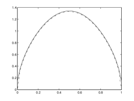
Figure 11: Dependence on number of terms in Fourier series for $u_{0}$ at $y=a$. Solid line from $y\leq a$ expansion. Dashed line from $y\geq a$ expansion. (a) $N=2$, (b) $N=40$

$N$	2	5	10	20	40
$\Omega_{0}$	0.2085	0.2101	0.2106	0.2108	0.2109
$\Omega_{0}$	0.6244	0.6290	0.6305	0.6312	0.6315
$\Omega_{0}$	1.0355	1.0431	1.0454	1.0466	1.0471
$\Omega_{0}$	1.4307	1.4404	1.4433	1.4447	1.4454

Table 2: The four standing wave frequencies for the comb-like structure with $a=7$ calculated from Fourier series expansion with the convergence shown by increasing the modes used.

$N$	2	5	10	20	40
$T$	-0.0068	-0.0066	-0.0066	-0.0066	-0.0066
$T$	-0.0704	-0.0687	-0.0686	-0.0686	-0.0686
$T$	-0.2877	-0.2843	-0.2849	-0.2856	-0.2860
$T$	-2.2022	-2.3602	-2.4267	-2.4628	-2.4816

Table 3: The values of $T$ associated with the four standing wave frequencies for the comb-like structure with $a=7$ calculated from Fourier series expansion with with the convergence shown by increasing the modes used.

The calculations of the standing wave frequencies and the coefficient $T$ are shown in tables  2 and 3 for different values of $N$ between 2 and 40 and demonstrate that these values are relatively insensitive to the value of $N$ used. There is good agreement with the values obtained from the full numerical simulation and the asymptotic approximation.

In Table 1 the values of $T$ used in equation (19), which combined with the standing wave ($\Omega_{0}$) and excitation ($\Omega$) frequencies yield an effective medium equation. Fig. 4 shows the appearance of a new length scale when a periodic comb-like structure with $a=7$, is excited with a line source at the frequencies of $\Omega=0.4509$ and $\Omega=1.3138$ respectively in Fig. 4 (a) and (b). The standing wave eigensolutions closest to these frequencies are shown in Fig. 3(a), (b) and show that on the microscale one expects no oscillation or one oscillation along the open waveguide formed by the comb teeth in one strip, and this local behaviour is indeed seen in Fig. 4. There is also clearly a long-scale oscillation along the comb and the calculation of the apparent pseudo wavelength is possible by HFH as explained in section 22.2 and yields the respective wavelengths $\lambda/2\sim 43.4$ and $\lambda/2\sim 73$. These are in accordance with panels (a) and (b) of Figs. 4 and 5 where the latter shows a complete reproduction by HFH of the numerical results, obtained by plotting Real$(u)$.

3.2 Array of cylinders

Similarly to the comb structure one can also have a diffraction grating constructed from a linear array of obstacles where surface wave modes can again occur. We consider a linear periodic array of cylinders, as in say Evans & Porter (1998), where Rayleigh-Bloch modes are observed.

The first mode, which is symmetric about $y=0$, is shown in Fig. 6(b) and exists for all radii $r_{0}$ of the cylinders such that $r_{0}\in]0,1[$. Fig. 6(a) shows the dispersion branches for radii $r_{0}=0.4$, $0.5$ and $0.7$ and the associated HFH asymptotics. If the radius is greater than $r_{0}\sim 0.81$ a second Rayleigh-Bloch mode appears, illustrated in Fig. 7(b), which is anti-symmetric about $y=0$. To motivate how this occurs we turn to a two-dimensional rectangular lattice of cylinders, as a generalization of Antonakakis et al. (2013), so instead of a grating we consider the dispersion diagram of a doubly periodic structure where the width of the rectangles is fixed to $2$ and the height is gradually increased until a grating-like strip is obtained. Fig. 8(a), (b) and (c) show the first three modes, and the light line $\Omega=\kappa$, for the respective cell heights of $h=2$, $6$ and $30$ and each with a centered hole of radius $r_{0}=0.95$. Both dispersion modes initially above the light line converge to the latter as the height of the cell increases and eventually one emerges beneath it. Upon inspection the Bloch mode, for the rectangular array, that passes beneath the light line has the appropriate symmetry and limits to the anti-symmetric mode for the grating. As discussed in Evans & Porter (1998) the critical radius value is $\sim 0.81$ and beyond this there is the emergence of the antisymmetric trapped mode; this is illustrated in Fig. 8(d) which shows the anti-symmetric mode, for a rectangular array height of $h=30$, for radii $r_{0}=0.4$, $0.81$ and $0.95$ respectively. For radii $r_{0}=0.4$ and $0.81$ the mode merges with the light line, but the mode related to $0.95$ emerges below the light line and one then observes this anti-symmetric Rayleigh Bloch mode. For all radii less than $\sim 0.81$ all modes, bar the first, will collapse on the lightline. Fig. 8(e) shows a summary of the variation of the standing wave frequencies with radius, and the appearance of this anti-symmetric mode for radii in the interval $[0.81,1[$ is evident. Notably, the asymptotic HFH theory captures the behaviour of the dispersion curves in this case too as shown in Fig. 7(a).

To illustrate further HFH and the emergence of the long-scale oscillation we performed large-scale finite element simulations summarised in Fig. 9. The asymmetric mode was generated using a dipole source, to trigger the asymmetry, and the symmetric mode using a line source. The chosen frequencies are slightly away from the standing wave frequencies and are respectively $\Omega=1.508$ and $\Omega=1.38$ for panels (a) and (b). Once again the apparent lengthscales are evaluated by HFH to be $\lambda/2=109.4$ and $\lambda/2=72.7$ which are confirmed by the numerics as well as in Fig. 10.

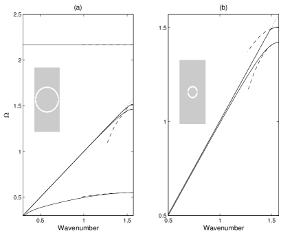
Figure 12: The dispersion branches for the SRR structure. Results from numerical simulations shown as solid lines, the asymptotics as dashed and the light line is dotted. Panel (a) is for a large SRR of outer radius $R_{out}=0.95$ and inner radius $R_{in}=0.85$ and panel (b) is for a smaller SRR with $R_{out}=0.4$ and $R_{in}=0.3$.

$T$	$\Omega_{0}$
$-0.145181377783699$	$0.550884858382472$
$-12.037628085319582$	$1.465518146041600$
$-25.144195967619925$	$1.517732423423271$
$-0.003773469173013$	$2.167224509645187$

Table 4: The four standing wave frequencies, below the cutoff, for a SRR grating with $R_{out}=0.95$ and $R_{in}=0.85$, c.f. Fig. 12(a), together with associated values for $T$.

Figure 13: The eigenfunctions $U_{0}$, and $U_{1}$ shown for the SRR structure, with outer, inner radius $R_{out}=0.95$, $R_{in}=0.85$ c.f. Fig. 12(a). These are for the $\Omega_{0}$ in Table 4 with (a)-(d) for ascending $\Omega_{0}$. In each panel $U_{0}$ is shown on the left and $U_{1}$ on the right.

3.3 Array of Split Ring Resonators

SRR are extensively used to achieve left handed materials used in electromagnetism Ramakrishna (2005). For SRRs here we choose to use a simple cylindrical annulus with two ligaments connecting the inner cylinder to the outer material. The weak coupling between the inner cylinder through these two thin ligaments is important as this arrangement can act as local resonators and this micro-resonance is important in photonic applications and in metamaterials Pendry et al. (1999). In SRR gratings Rayleigh-Bloch modes occur at frequencies above the cutoff due to this resonance behaviour within the inner part of the SRR as shown in the fourth mode of Figs. 12(a) and the resonance is clear in the eigensolution shown in 13(d). The ultra-flat dispersion curve, Fig. 12(a), is associated with dipole localized modes in every SRR of the grating and it can be predicted using a geometric asymptotic technique discussed in Antonakakis et al. (2013); Movchan & Guenneau (2004).

The modes that arise for the grating of SRR split into two families, one which is very similar to those of the cylinders of the last section, that is, Fig. 13(b) and (c) are respectively similar to those of Figs. 6(b) and 7(b). The lowest mode, whose eigensolution is shown in Fig. 13(a), is again one primarily associated with the inner cylinder and vibrations of the ligaments.

HFH is used to generate the asymptotics and Table 4 shows the standing wave frequencies and respective values of $T$ for the first four modes of a SRR grating with outer radius of $R_{out}=0.95$. The asymptotics of the dispersion curves again show pleasing accuracy.

Numerical finite element solutions for line source excitation show plainly this separation into exterior modes akin to those of the cylinder Figs. 14(a,b,c) and those localised almost entirely within the SRR as in Figs 14(d,e,f): In these latter cases the array acts very clearly as an oscillating string. The smaller SRR illustrated in Fig 15 gives an even more pronounced locally anti-periodic oscillation with long-scale oscillation. The excitation frequencies are chosen to be close to those of standing waves and the long-scale behaviour extracted using HFH as seen in the Fig. 16. The wavelengths associated with Fig. 16 are in the panel’s order of appearance, $\lambda/2=51.2,11,69.6,119.1$.

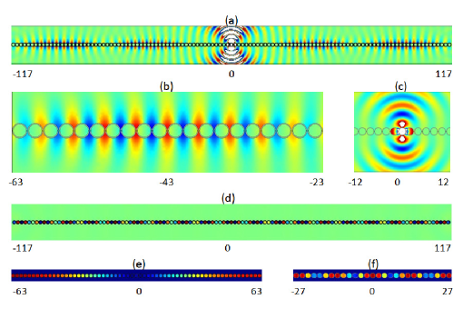
Figure 14: Plots of real $(u)$ for a SRR grating with SRR of inner and outer radii $0.85$ and $0.95$ respectively and ligaments of thickness $0.06$ (standing wave frequencies in Table 4): (a) Field generated by a line source at $\Omega=1.45$; (b,c) Detail of real $(u)$ at $\Omega=1.45$ centered around $x=-43$ showing the developed field (b) and around the source (c); (d) Field generated by a line source at $\Omega=0.54$; (e,f) Close up on the absolute value of field $u$ at frequency $\Omega=0.55,\Omega=0.54$ respectively.

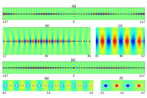
Figure 15: Plots of real $(u)$ for a SRR grating with SRR of inner and outer radii $0.3$ and $0.4$ and ligamets of thickness $0.06$: (a) Fields generated by a line source at $\Omega=1.50$ ($\Omega_{0}=1.50295$); (b,c) Detail of $u$ at $\Omega=1.50$ centered around $x=49$ showing the developed field ; (d) Field generated by a line source at $\Omega=1.42$ ($\Omega_{0}=1.42199$); (e,f) Detail of real $(u)$ at frequency $\Omega=1.42$

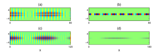
Figure 16: Panels (a) and (b) show real $(u)$ from HFH for a SRR, with inner and outer radii of $R_{in}=0.85$ and $R_{out}=0.95$, c.f. Fig. 14, generated by a line source at $\Omega=1.45$ and $\Omega=0.54$ respectively. Panels (c) and (d) show real $(u)$ from HFH for a SRR, with inner and outer radii of $R_{in}=0.3$ and $R_{out}=0.4$, c.f. Fig. 15, generated by a line source at $\Omega=1.50$ and $\Omega=1.42$ respectively.

4 Defect states in quasi periodic gratings

The previous examples illustrate HFH for perfectly periodic media but its applications go further than this. In section 3 HFH asymptotics and the resulting effective media successfully homogenise perfect periodic arrays, but one could also obtain analytical or numerical solutions fairly quickly at least for simple geometries. The real power of HFH lies in its capability to move away from perfect periodicity, we now take the comb of section 33.1, but now vary the height of the comb’s teeth with respect to the $x$ coordinate by a function $g(X)$, so that their height is $a(1-\epsilon^{2}g(X))$ and ask the question of whether localized states exist at specific frequencies in such quasi-periodic media, that is, are there finite energy states that have exponential decay along the array? We make the following change of coordinates in order to transform the varying tooth height in $x_{2}$ to constant height pins in the new coordinate $\xi_{2}$ such that,

$$\xi_{1}=\frac{x_{1}}{l}\text{,}\quad X=\frac{x_{1}}{L}\text{,}\quad\xi_{2}=\frac{x_{2}}{l}\left[1-\epsilon^{2}g(X)\right].$$ (28)

This sleight of hand transforms the medium and moves the tooth heights to a constant within this transformed medium. Following through the asymptotic procedure, as in section 2, we obtain three equations ordered in $\epsilon$, the only change is at second order where (7) becomes

$$u_{2,\xi_{i}\xi_{i}}+\Omega_{0}^{2}u_{2}=-u_{0,XX}-2u_{1,\xi_{1}X}+2g(X)u_{0,\xi_{2}\xi_{2}}-\Omega_{1}^{2}u_{1}-\Omega_{2}^{2}u_{0}$$ (29)

which contains an additional term. Neumann boundary conditions remain unchanged for leading and first order but in second order yield,

$$u_{1,X}n_{1}+u_{2,\xi_{i}}n_{i}-g(X)u_{0,\xi_{2}}n_{2}=0.$$ (30)

Using a solvability condition we obtain an equation for $f_{0}$ as,

$$Tf_{0,XX}+f_{0}[\alpha g(X)+\Omega_{2}^{2}]=0,\quad\text{with}\quad\alpha=\frac{\int\int_{S}(U_{0,\xi_{2}}^{2}-U_{0}U_{0,\xi_{2}\xi_{2}})dS}{\int\int_{S}U_{0}^{2}dS},$$ (31)

where $T$ is given in (15). This is a Schroedinger equation and for specific choices of $g(X)$ exact solutions exist notably for $g(X)=-{\rm sech}^{2}X$ as in Infeld & Hull (1951); Craster et al. (2010b), hence adopting this variation an asymptotic value of the lowest defect mode frequency is explicitly

$$\Omega^{2}=\Omega_{0}^{2}-\frac{T\epsilon^{2}}{4}\left(1-\sqrt{1-4\alpha/T}\right)^{2}$$ (32)

provided that $\alpha/T$ is always negative, which occurs as $T$ is always negative and $\alpha$ positive. The associated solutions for $f_{0}(X)$ are Infeld & Hull (1951),

$$f_{0}(X)=\pi^{-\frac{1}{4}}\bigg{(}\frac{\Gamma(\gamma)}{\Gamma(\gamma-1/2)}\bigg{)}^{\frac{1}{2}}{\rm cosh}^{-\gamma+1/2}X,$$ (33)

where for the lowest defect mode $\gamma=\sqrt{1/4-\alpha/T}$ and $\Gamma(\gamma)$ is the Gamma function Abramowitz & Stegun (1964).

For $a=7$ Table 5 shows the predictions of the frequencies at which these defect states arise versus values extracted from finite element simulations which are reassuringly accurate, and these defect mode frequencies are above the standing wave frequencies as one would expect. Perhaps more compelling are the illustrative solutions shown in Fig. 17 which show $f_{0}$ versus the numerical eigensolutions; as both solutions are arbitrary to within a multiplicative constant we normalise to have $\max(f_{0})$ equal to the maximum value from the numerics.

$\epsilon$	$\Omega_{HFH}$	$\Omega_{num}$
$0.125$	$0.21247$	$0.21252$
$0.0625$	$0.21074$	$0.21079$

Table 5: The predicted frequencies of the localized defect mode near the first standing wave frequency ($\Omega_{0}=0.210161050669707$, c.f. Table 1) for the comb-like structure with $a=7$ c.f. Fig. 2(d). The frequencies $\Omega_{HFH}$ come from the asymptotics (32) whereas $\Omega_{num}$ gives predictions from FEM simulations. The parameter $\epsilon$ controls the variation of tooth height in (28).

Figure 17: The localized defect mode shown for the comb-like structure withvariation of tooth height for $a=7$. The variation follows equation (28) with $\epsilon=0.125$ in panel (a) and $\epsilon=0.0625$ in panel (b). In solid are solutions from FEM simulations of $u$ along $x$ and for $y=7$, and in dashed are from equation (33).

5 Concluding remarks

It is shown here that one can take a microstructured surface, or diffraction grating Popov (2012); Petit (1980), and close to the standing wave frequencies that occur, one can represent the surface as an effective string, or membrane. The standing waves can occur at high frequencies and as a result the effective stiffness is not simply an average but involves the integrals over a microscale, importantly the effective equation is posed entirely on the long-scale with the short-scale built in through integrated quantities. Thus we extend homogenization in two distinct directions enabling microstructed surfaces, instead of the more usual bulk media, to be modelled and away from the usual low-frequency limit. Given the effective equation description one can then concentrate numerical efforts on modeling instead of capturing the fine scale detail. Indeed, as shown in section 4, one can use the effective description to capture analytically features such as defect states caused by non-periodic behaviour.

There are several practical directions that could be pursued using this analysis, notably the surface wave for line source excitation demonstrates the two-scale behaviour beautifully with a short-scale oscillation from one neighbouring strip to the next and, in some sense, chooses its own longer wavelength. The current theory neatly encapsulates this and this information could be used as part of an inverse problem to determine the quality of microscale or nanoscale surfaces, and the defect states could identify local damage. Importantly, questions related to tuning a surface to have designer properties can be encapsulated into how the coefficient $T$ behaves and that too avoids lengthy computations using numerical methods for gratings such as Fourier Li (1996) or differential Lalanne (1997) methods.

In summary, one can now take a microstructured surface, or diffraction grating, that is periodic, or nearly so, and replace it by a continuum description that captures the surface Rayleigh-Bloch waves.

References

- Abramowitz & Stegun (1964) Abramowitz, M. & Stegun, I. A. 1964 Handbook of Mathematical Functions. Washington: National Bureau of Standards.
- Allaire & Piatnitski (2005) Allaire, G. & Piatnitski, A. 2005 Homogenisation of the Schrödinger equation and effective mass theorems. Commun. Math. Phys. 258, 1–22.
- Antonakakis & Craster (2012) Antonakakis, T. & Craster, R. V. 2012 High frequency asymptotics for microstructured thin elastic plates and platonics. Proc. R. Soc. Lond. A 468, 1408–1427.
- Antonakakis et al. (2013) Antonakakis, T., Craster, R. V. & Guenneau, S. 2013 Asymptotics for metamaterials and photonic crystals. Proc. R. Soc. Lond. A 469, 20120533.
- Bakhvalov & Panasenko (1989) Bakhvalov, N. & Panasenko, G. 1989 Homogenization: Averaging Processes in Periodic Media. Amsterdam: Kluwer.
- Barlow & Karbowiak (1954) Barlow, H. E. M. & Karbowiak, A. E. 1954 An experimental investigation of the properties of corrugated cylindrical surface waveguides. Proc. IEE 101, 182–188.
- Bensoussan et al. (1978) Bensoussan, A., Lions, J. & Papanicolaou, G. 1978 Asymptotic analysis for periodic structures. North-Holland, Amsterdam.
- Birman & Suslina (2006) Birman, M. S. & Suslina, T. A. 2006 Homogenization of a multidimensional periodic elliptic operator in a neighborhood of the edge of an internal gap. Journal of Mathematical Sciences 136, 3682–3690.
- Bonnet-Bendhia & Starling (1994) Bonnet-Bendhia, A. S. & Starling, F. 1994 Guided waves by electromagnetic gratings and nonuniqueness examples for the diffraction problem. Math. Meth. Appl. Sci. 17, 305–338.
- Brekhovskikh (1959) Brekhovskikh, L. M. 1959 Surface waves in acoustics. Sov. Phys. Acoust. 5, 3–12.
- Conca et al. (1995) Conca, C., Planchard, J. & Vanninathan, M. 1995 Fluids and Periodic structures. Res. Appl. Math., Masson, Paris.
- Craster et al. (2013) Craster, R. V., Joseph, L. M. & Kaplunov, J. 2013 Long-wave asymptotic theories: The connection between functionally graded waveguides and periodic media. Under review.
- Craster et al. (2011) Craster, R. V., Kaplunov, J., Nolde, E. & Guenneau, S. 2011 High frequency homogenization for checkerboard structures: Defect modes, ultra-refraction and all-angle-negative refraction. J. Opt. Soc. Amer. A 28, 1032–1041.
- Craster et al. (2010a) Craster, R. V., Kaplunov, J. & Pichugin, A. V. 2010a High frequency homogenization for periodic media. Proc R Soc Lond A 466, 2341–2362.
- Craster et al. (2010b) Craster, R. V., Kaplunov, J. & Postnova, J. 2010b High frequency asymptotics, homogenization and localization for lattices. Q. Jl. Mech. Appl. Math. 63, 497–519.
- DeSanto (1972) DeSanto, J. A. 1972 Scattering from a periodic corrugated structure II. Thin comb with hard boundaries. J. Math. Phys. 13, 336–341.
- Enoch & Bonod (2012) Enoch, S. & Bonod, N. 2012 Plasmonics: From Basics to Advanced Topics. Springer Series in Optical Sciences, Vol. 167.
- Evans & Linton (1993) Evans, D. V. & Linton, C. M. 1993 Edge waves along periodic coastlines. QJMAM 46, 643–656.
- Evans & Porter (1998) Evans, D. V. & Porter, R. 1998 Trapping and near-trapping by arrays of cylinders in waves. J. Engng Math. 35, 149–179.
- Evans & Porter (2002) Evans, D. V. & Porter, R. 2002 On the existence of embedded surface waves along arrays of parallel plates. QJMAM 55, 481–494.
- Fernandez-Dominguez et al. (2011) Fernandez-Dominguez, A. I., Garcia-Vidal, F. & Martin-Moreno, L. 2011 Structured surfaces as optical metamaterials, Ed. A. A. Maradudin, chap. Surface electromagnetic waves on structured perfectly conducting surfaces. CUP.
- Gridin et al. (2004) Gridin, D., Adamou, A. T. I. & Craster, R. V. 2004 Electronic eigenstates in quantum rings: Asymptotics and numerics. Phys Rev B 69, 155317.
- Gridin et al. (2005) Gridin, D., Craster, R. V. & Adamou, A. T. I. 2005 Trapped modes in curved elastic plates. Proc R Soc Lond A 461, 1181–1197.
- Hoefer & Weinstein (2011) Hoefer, M. A. & Weinstein, M. I. 2011 Defect modes and homogenization of periodic Schrödinger operators. SIAM J. Math. Anal. 43, 971–996.
- Hurd (1954) Hurd, R. A. 1954 The propagation of an electromagnetic wave along an infinite corrugated surface. Can. J. Phys. 32, 727–734.
- Infeld & Hull (1951) Infeld, L. & Hull, T. E. 1951 The factorization method. Rev. Modern Phys. 23, 21–68.
- Joannopoulos et al. (2008) Joannopoulos, J. D., Johnson, S. G., Winn, J. N. & Meade, R. D. 2008 Photonic Crystals, Molding the Flow of Light, 2nd edn. Princeton University Press, Princeton.
- Joseph & Craster (2013) Joseph, L. M. & Craster, R. V. 2013 Asymptotics for Rayleigh-Bloch waves along lattice line defects. Multiscale Modeling and Simulation.
- Kaplunov et al. (2005) Kaplunov, J. D., Rogerson, G. A. & Tovstik, P. E. 2005 Localized vibration in elastic structures with slowly varying thickness. Quart. J. Mech. Appl. Math. 58, 645–664.
- Lalanne (1997) Lalanne, P. 1997 Convergence performance of the coupled-wave and the differential method for thin gratings. J. Opt. Soc. Am. A 14, 1583–1591.
- Li (1996) Li, L. 1996 Use of Fourier series in the analysis of discontinuous periodic structures. J. Opt. Soc. Am. A 13, 1870–1876.
- Linton & McIver (2002) Linton, C. M. & McIver, M. 2002 The existence of Rayleigh-Bloch surface waves. J. Fluid Mech. 470, 85–90.
- Maier (2007) Maier, S. A. 2007 Plasmonics: Fundamentals and Applications. Springer-Verlag.
- Makwana & Craster (2012) Makwana, M. & Craster, R. V. 2012 Localized defect states for high frequency homogenized lattice models. Quart. J. Mech. Appl. Math. To appear: doi:10.1093/qjmam/hbt005.
- Maniar & Newman (1997) Maniar, H. D. & Newman, J. N. 1997 Wave diffraction by a long array of cylinders. J. Fluid Mech. 339, 309–330.
- McIver et al. (1998) McIver, P., Linton, C. M. & McIver, M. 1998 Construction of trapped modes for wave guides and diffraction gratings. Proc. R. Soc. Lond. A 454, 2593–2616.
- Movchan & Guenneau (2004) Movchan, A. B. & Guenneau, S. 2004 Split-ring resonators and localized modes. Phys. Rev. B 70, 125116.
- Nemat-Nasser et al. (2011) Nemat-Nasser, S., Willis, J. R., Srivastava, A. & Amirkhizi, A. V. 2011 Homogenization of periodic elastic composites and locally resonant sonic materials. Phys. Rev. B 83, 104103.
- Nevard & Keller (1997) Nevard, J. & Keller, J. B. 1997 Homogenization of rough boundaries and interfaces. SIAM J. Appl. Math. 57, 1660–1686.
- Nolde et al. (2011) Nolde, E., Craster, R. V. & Kaplunov, J. 2011 High frequency homogenization for structural mechanics. J. Mech. Phys. Solids 59, 651–671.
- Panasenko (2005) Panasenko, G. 2005 Multi-scale modelling for structures and composites. Dordrecht: Springer.
- Pendry et al. (1999) Pendry, J. B., Holden, A. J., Stewart, W. J. & Youngs, I. 1999 Magnetism from conductors and enhanced nonlinear phenomena. IEEE Trans. Micr. Theo. Tech. 47, 2075.
- Pendry et al. (2004) Pendry, J. B., Martin-Moreno, L. & Garcia-Vidal, F. J. 2004 Mimicking surface plasmons with structured surfaces. Science 305, 847–848.
- Petit (1980) Petit, R. 1980 Electromagnetic theory of gratings, Topics in current physics. Springer-Verlag, Berlin.
- Popov (2012) Popov, E. 2012 Gratings: Theory and Numerical Applications. Aix-Marseille University.
- Porter & Evans (1999) Porter, R. & Evans, D. V. 1999 Rayleigh-Bloch surface waves along periodic gratings and their connection with trapped modes in waveguides. J. Fluid Mech. 386, 233–258.
- Ramakrishna (2005) Ramakrishna, S. A. 2005 Physics of negative refractive index materials. Rep. Prog. Phys. 68, 449–521.
- Sanchez-Palencia (1980) Sanchez-Palencia, E. 1980 Non-homogeneous media and vibration theory. Berlin: Springer-Verlag.
- Sengupta (1959) Sengupta, D. 1959 On the phase velocity of wave propagation along an infinite Yagi structure. IRE Trans. Antennas Propagat 7, 234–239.
- Wilcox (1984) Wilcox, C. H. 1984 Scattering theory for diffraction gratings. Springer-Verlag.