Optimal Recombination in Genetic Algorithms

Abstract

This paper surveys results on complexity of the optimal recombination problem (ORP), which consists in finding the best possible offspring as a result of a recombination operator in a genetic algorithm, given two parent solutions. We consider efficient reductions of the ORPs, allowing to establish polynomial solvability or NP-hardness of the ORPs, as well as direct proofs of hardness results.

Keywords:
1) Genetic Algorithm
2) Optimal Recombination
3) Complexity
4) Crossover

1 Introduction

The genetic algorithms (GAs) originally suggested by J. Holland [32] are randomized heuristic search methods using an evolving population of sample solutions, based on analogy with the genetic mechanisms in nature. Various modifications of GAs have been widely used in operations research, pattern recognition, artificial intelligence, and other areas (see e.g. [43, 49, 50]). Despite numerous experimental studies of these algorithms, the theoretical analysis of their efficiency is currently at an early stage [11]. Efficiency of GAs depends significantly on the choice of crossover operator, that combines the given parent solutions, aiming to produce "good" offspring solutions (see e.g. [34]). Originally the crossover operator was proposed as a simple randomized procedure [32], but subsequently the more elaborated problem-specific crossover operators emerged [43].

This paper is devoted to complexity and solution methods of the Optimal Recombination Problem (ORP), which consists in finding the best possible offspring as a result of a crossover operator, given two feasible parent solutions. The ORP is a supplementary problem (usually) of smaller dimension than the original problem, formulated in view of the basic principles of crossover [42].

The first GAs using the optimal recombination appeared in the works of C.C. Agarwal, J.B. Orlin and R.P. Tai [1] and M. Yagiura and T. Ibaraki [49]. These works provide GAs for the Maximum Independent Set problem and several permutation problems. Subsequent results in [8, 16, 19, 24, 27] and other works added more experimental support to expediency of solving the optimal recombination problems in crossover operators.

Interestingly, it turned out that a number of NP-hard optimization problems have efficiently solvable ORPs. The present paper contains a survey of results focused on the issue of efficient solvability vs. intractability of the ORPs.

The paper is structured as follows. The formal definition of the ORP for NP optimization problems is introduced in Section 2. Then, using efficient reductions between the ORPs it is shown in Section 3 that the optimal recombination is computable in polynomial time for the Maximum Weight Set Packing Problem, the Minimum Weight Set Partition Problem and for one of the versions of the Simple Plant Location Problem. In Section 3 we also propose an efficient optimal recombination operator for the Boolean Linear Programming Problems with at most two variables per inequality. In Section 4 we consider a number of NP-hard ORPs for the Boolean Linear Programming Problems. The computational complexity of ORP for the Travelling Salesman Problem is considered in Section 5 both for the symmetric and for the general case. Strong NP-hardness of these optimal recombination problems is proven and solving approaches are proposed. A closely related problem of Makespan Minimization on Single Machine is considered in Section 6: it is shown that on one hand this ORP problem is strongly NP-hard, on the other hand, almost all of its instances are efficiently solvable. Section 7 is devoted to the concluding remarks and issues for further research.

2 Optimal Recombination in Genetic Algorithms

We will employ the standard definition of an NP optimization problem (see e.g. [5]). By $\{0,1\}^{*}$ we denote the set of all strings with symbols from $\{0,1\}$ and arbitrary string length. For a string $S\in\{0,1\}^{*}$, the symbol $|S|$ will denote its length. The term polynomial time stands for the computation time which is upper bounded by a polynomial in length of the input data. Let ${\mathbb{R}}_{+}$ denote the set of non-negative reals.

Definition 1

An NP optimization problem $\Pi$ is a triple ${\Pi=(\mbox{\rm Inst},\mbox{\rm Sol},f_{I})}$, where $\mbox{\rm Inst}\subseteq\{0,1\}^{*}$ is the set of instances of $\Pi$ and:

1. The relation Inst is computable in polynomial time.

2. Given an instance $I\in\mbox{\rm Inst}$, $\mbox{\rm Sol}(I)\subseteq\{0,1\}^{n(I)}$ is the set of feasible solutions of $I$, where $n(I)$ stands for the dimension of the space of solutions. Given $I\in\mbox{\rm Inst}$ and $\mbox{\bf x}\in\{0,1\}^{n(I)}$, the decision whether $\mbox{\bf x}\in\mbox{\rm Sol}(I)$ may be done in polynomial time, and $n(I)\leq\mbox{\rm poly}(|I|)$ for some polynomial poly.

3. Given an instance $I\in\mbox{\rm Inst}$, $f_{I}:\mbox{\rm Sol}(I)\to{\mathbb{R}}_{+}$ is the objective function (computable in polynomial time) to be maximized if $\ \Pi$ is an NP maximization problem or to be minimized if $\ \Pi$ is an NP minimization problem.

For the sake of compactness of notation we will simply put ${\rm Sol}$ instead of ${\rm Sol}(I)$, $n$ instead of $n(I)$ and $f$ instead of $f_{I}$, when it is clear what problem instance is implied.

Throughout the paper we use the term efficient algorithm as a synonym for polynomial-time algorithm. A problem which is solved by such an algorithm is polynomially solvable.

Often it is possible to formulate an NP optimization problem as a Boolean Linear Programming Problem:

$$\mbox{max}\ \ f(\mbox{\bf x})=\sum_{j=1}^{n}c_{j}x_{j},$$ (1)

subject to

$$\sum_{j=1}^{n}a_{ij}x_{j}\leq b_{i},\quad i=1,\dots,m,$$ (2)

$$x_{j}\in\{0,1\},\quad j=1,\dots,n.$$ (3)

In the context of Boolean Linear Programming Problem, $\mbox{\bf x}\in\{0,1\}^{n}$ is treated as a column vector of Boolean variables $x_{1},\dots,x_{n}$, which belongs to ${\rm Sol}$ iff the constraints (2) are satisfied. The similar problems where instead of "$\leq$" in (2) stands "$\geq$" or "$=$" for some indices $i$ (or for all $i$) can be easily transformed to formulation (1)–(3). The minimization problems can be considered, using the goal function with coefficients $c_{j}$ of opposite sign. Where appropriate, we will use a more compact notation for problem (1)–(3):

$$\max\left\{{\bf cx}:{\bf Ax}\leq{\bf b},\ {\bf x}\in\{0,1\}^{n}\right\},$$

where A is an ($m\times n$)-matrix with elements $a_{ij}$, ${\bf b}=(b_{1},\dots,b_{m})^{T}$ and ${\bf c}=(c_{1},\dots,c_{n})$.

2.1 Genetic Algorithms

The simple GA proposed in [32] has been intensively studied and exploited over four decades (see e.g. [44]). This algorithm operates with populations $X^{t},\ t=1,2,\dots$ of binary strings in $\{0,1\}^{n}$ traditionally called genotypes. Each population consists of a fixed number of genotypes $N$, which is assumed to be even. In a selection operator ${\rm Sel}$, each parent is drawn from the previous population $X^{t}$ independently with probability distribution assigning each genotype a probability proportional to its fitness, where fitness is measured by the value of the objective function or a composition of the objective function with some monotonic function.

A pair of offspring genotypes is created through recombination and mutation stages (see Fig 1). In the recombination stage, a crossover operator ${\rm Cross}$ exchanges random substrings between pairs of parent genotypes $\xi,\eta$ with a given constant probability $P_{\rm c}$ so that

$${\bf P}\left\{\xi^{\prime}=(\xi_{1},...,\xi_{j},\eta_{j+1},...,\eta_{n}),\ \eta^{\prime}=(\eta_{1},...,\eta_{j},\xi_{j+1},...,\xi_{n})\right\}=\frac{P_{\rm c}}{n-1},\ j=1,...,n-1,$$

$${\bf P}\{\xi^{\prime}=\xi,\ \eta^{\prime}=\eta\}=1-P_{\rm c}.$$

In the mutation operator ${\rm Mut}$, each bit of an offspring genotype may be flipped with a constant mutation probability $P_{\rm m}$, which is usually chosen relatively small. When the whole population $X^{t+1}$ of $N$ offspring is constructed, the GA proceeds to the next iteration $t+1$. An initial population $X^{0}$ is generated randomly with independent choice of all bits in genotypes.

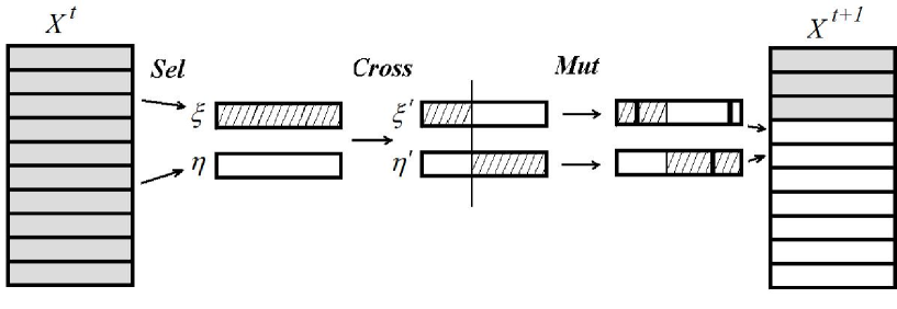
Figure 1: Selection, crossover and mutation in Simple Genetic Algorithm.

A plenty of variants of GA have been developed since publication of the simple GA in [32], sharing the basic ideas, but using different population management strategies, selection, crossover and mutation operators [44]. The practice shows that the best results are obtained when the GAs are designed in view of the specific features of the optimization problem to be solved. A number of such problem-specific GAs make use of crossover operators that find exact or at least approximate solution to the optimal recombination problem.

2.2 Formulation of Optimal Recombination Problem

In this paper, the ORPs are considered assuming binary representation of solutions in genotypes being identical to the solutions encoding of the NP optimization problem. Besides that, it will be assumed that $X^{0}$ consists of feasible solutions and operators ${\rm Cross}$ and ${\rm Mut}$ maintain feasibility of solutions, i. e. ${\rm Cross}:{\rm Sol}^{2}\to{\rm Sol}^{2},\ {\rm Mut}:{\rm Sol}\to{\rm Sol}$. Therefore the term "genotype" will mean an element of the set of feasible solutions ${\rm Sol}$.

Note that there may be a number of NP optimization problems, essentially corresponding to the same problem in practice. Such formulations are usually easy to transform to each other but the solution representations may be quite different in the degree of degeneracy, the number of local optima for some standard neighborhood definitions, the length of encoding strings and other parameters important for heuristic algorithms. Since the method of solutions representation is crucial for recombination operators, in what follows we will always explicitly indicate what solutions encoding is used in formulation of an NP optimization problem.

In general, an instance of an NP optimization problem may have no feasible solutions. However, w.r.t. the optimal recombination problem such cases are not meaningful, since there exist no feasible parent solutions. Therefore, in the context of optimal recombination below we will always assume that ${\rm Sol}\neq\emptyset$.

The following definition of optimal recombination problem is motivated by the principles of (strictly) gene transmitting recombination formulated by N. Radcliffe [42].

Definition 2

Given an NP optimization problem $\Pi=(\mbox{\rm Inst},{\rm Sol},f)$, the optimal recombination problem for $\Pi$ is the NP optimization problem $\overline{\Pi}=(\overline{\rm Inst},\overline{\rm Sol},\overline{f})$, where for every instance ${\overline{I}=(I,{\bf p}^{1},{\bf p}^{2})\in\overline{\rm Inst}}$ holds $I\in{\rm Inst}$, ${{\bf p}^{1}=(p_{1}^{1},\dots,p_{n(I)}^{1})\in{\rm Sol}(I)},\ {{\bf p}^{2}=(p_{1}^{2},\dots,p_{n(I)}^{2})\in{\rm Sol}(I)}$, and it is assumed that

$$\overline{\rm Sol}(\overline{I})=\{\mbox{\bf x}\in{\rm Sol}(I)|\ x_{j}=p^{1}_{j}\ \mbox{or}\ x_{j}=p^{2}_{j},\ j=1,\dots,{n(I)}\}.$$ (4)

The optimization criterion in $\overline{I}$ is the same as in $I$, i. e.  $\overline{f}_{\overline{I}}\equiv f_{I}$.

The feasible solutions ${\bf p}^{1},{\bf p}^{2}$ to problem $I$ are called the parent solutions for the problem $\overline{I}=(I,{\bf p}^{1},{\bf p}^{2})$. In what follows, we denote the set of coordinates, where the parent solutions have different values, by $D(\mbox{\bf p}^{1},\mbox{\bf p}^{2})=\{j:p^{1}_{j}\neq p^{2}_{j}\}.$ These are the variables subject to optimization in the ORP. All other variables are "fixed" in the ORP being equal to the values of the corresponding coordinates in the parent solutions.

Other formulations of recombination subproblem, that may be found in literature, are the examples of allelic dynastically optimal recombination [15]. In particular, in [12, 13, 21, 39] promising experimental results were demonstrated by GAs where the recombination subproblem is defined by "fixing" only those genes, where both parent genotypes contain zeros.

3 Efficiently Solvable Optimal Recombination Problems

As the first examples of efficiently solvable ORPs we will consider the following three well-known problems. Given a graph $G=(V,E)$ with vertex weights $w(v),\ v\in V$,

• the Maximum Weight Independent Set Problem asks for a subset ${S\subseteq V}$, such that each edge ${e\in E}$ has at least one endpoint outside $S$ (i.e. $S$ is an independent set) and the weight $\sum_{v\in S}w(v)$ of $S$ is maximized;

• the Maximum Weight Clique Problem asks for a maximum weight subset ${Q\subseteq V}$, such that any two vertices $u,v$ in $Q$ are adjacent (i. e. $Q$ is a clique);

• the Minimum Weight Vertex Cover Problem asks for a minimum weight subset ${C\subseteq V}$, such that any edge ${e\in E}$ is incident at least to one of the vertices in $C$ (i. e. $C$ is a vertex cover).

Suppose, the vertices of graph $G$ are ordered. We will consider these three problems using the standard binary representation of solutions by the indicator vectors, assuming $n=|V|$ and $x_{j}=1$ iff vertex $v_{j}$ belongs to the subset represented by x. The following result is due to E. Balas and W. Niehaus.

Theorem 1

[6] The ORP for the Maximum Weight Clique Problem is solvable in time ${O(|D(\mbox{\bf p}^{1},\mbox{\bf p}^{2})|^{3}+n)}$.

Proof. Consider the Maximum Weight Clique Problem on a given graph $G$ with two parent cliques $Q_{1}$ and $Q_{2}$, represented by binary vectors $\mbox{\bf p}^{1}$ and $\mbox{\bf p}^{2}$. An offspring solution $Q$ should contain the whole set of vertices $Q_{1}\cap Q_{2}$, besides that $Q$ should not contain the elements from the set $V\setminus(Q_{1}\cup Q_{2})$, while the vertices with indices from the set $D({\bf p}^{1},{\bf p}^{2})$ should be chosen optimally. The latter task can be formulated as a Maximum Weight Clique Problem in subgraph $H=(V^{\prime},E^{\prime})$, which is induced by the subset of vertices with indices from $D({\bf p}^{1},{\bf p}^{2})$. To find a clique of maximum weight in $H$, it is sufficient to find a minimum weight vertex cover $C^{\prime}$ in the complement graph $\bar{H}$ and take $V^{\prime}\backslash C^{\prime}$. Note that $\bar{H}$ is a bipartite graph, so let $V^{\prime}_{1},V^{\prime}_{2}$ be the subsets of vertices in this bipartition.

The Minimum Weight Vertex Cover $C^{\prime}$ for $\bar{H}$ can be found by solving the $s$-$t$-Minimum Cut Problem on a supplementary network ${\cal N}$, based on $\bar{H}$, as described e.g. in [30]: in this network, an additional vertex $s$ is connected by outgoing arcs with the vertices of set $V^{\prime}_{1}$, and the other additional vertex $t$ is connected by incoming arcs to the subset $V^{\prime}_{2}$. The capacities of the new arcs are equal to the weights of the adjacent vertices in $\bar{H}$. Each edge of $\bar{H}$ is viewed as an arc, directed from its endpoint $u\in V_{1}^{\prime}$ to the endpoint $v\in V_{2}^{\prime}$. The arc capacity is set to $\max\{w(u),w(v)\}$. This $s$-$t$-Minimum Cut Problem can be solved in ${O(|D(\mbox{\bf p}^{1},\mbox{\bf p}^{2})|^{3})}$ time using the maximum-flow algorithm due to A.V. Karzanov – see e.g. [40]. We will assume that the $s$-$t$-minimum cut contains only the arcs outgoing from $s$ or incoming into $t$, because if some arc $(u,v),$ $u\in V^{\prime}_{1},v\in V^{\prime}_{2}$ enters the $s$-$t$-minimum cut, one can substitute it by $(s,u)$ or $(v,t)$, and this will not increase the weight of the cut. Finally, it is easy to verify that $(V^{\prime}_{1}\cup V^{\prime}_{2})\backslash C^{\prime}$ joined with $Q_{1}\cap Q_{2}$ defines the required ORP solution. Since the parent solutions are given by the $n$-dimensional indicator vectors $\mbox{\bf p}^{1}$ and $\mbox{\bf p}^{2}$, we get the overall time complexity ${O(|D(\mbox{\bf p}^{1},\mbox{\bf p}^{2})|^{3}+n)}$. $\Box$

Note that if all vertex weights are equal, then the time complexity of Karzanov’s algorithm for the networks of simple structure (as the one constructed in the proof of Theorem 1) reduces to ${O(|D(\mbox{\bf p}^{1},\mbox{\bf p}^{2})|^{2.5})}$ – see [40].

The Maximum Weight Independent Set and the Minimum Weight Vertex Cover Problems are closely related to the Maximum Weight Clique Problem (see e.g. [26]). It is sufficient to consider the complement graph and to change the optimization criterion accordingly. Then there is a bijection between the set of feasible solutions of each of these problems and the set of feasible solutions of the corresponding Maximum Weight Clique Problem. In the case of Maximum Weight Independent Set, the bijection is an identity mapping, while in the case of the Minimum Weight Vertex Cover, the bijection alters each bit in x. In the first case the mapped feasible solutions retain thir objective function values, while in the second case the original objective function values are subtracted from the weight of all vertices. In view of these relationships Theorem 1 implies that the ORPs for the Maximum Weight Independent Set and the Minimum Weight Vertex Cover Problems are solvable in time ${O(|D(\mbox{\bf p}^{1},\mbox{\bf p}^{2})|^{3}+n)}$ as well. Indeed, it suffices to consider the corresponding instance of the ORP for the Maximum Clique Problem, solve this ORP in ${O(|D(\mbox{\bf p}^{1},\mbox{\bf p}^{2})|^{3}+n)}$ time and map the obtained solution back into the set of feasible solutions of the original problem.

The above arguments illustrate that when one NP-optimization problem transforms efficiently to another one, the corresponding ORPs may reduce efficiently as well. The following subsection is devoted to analysis of the situations where such arguments apply.

3.1 Reductions of Optimal Recombination Problems

The usual approach to spreading a class of polynomially solvable (or intractable) problems consists in building chains of efficient problem reductions. In order to apply this approach to optimal recombination problems we shall first formulate a relatively general reducibility condition for NP optimization problems.

Proposition 1

Let ${\Pi_{1}={({\rm Inst}_{1},{\rm Sol}_{1},f_{I})}}$ and $\Pi_{2}={({\rm Inst}_{2},{\rm Sol}_{2},g_{I^{\prime}})}$ be NP optimization problems with maximization (minimization) criteria and there exists a mapping ${\alpha:{\rm Inst}_{1}\to{\rm Inst}_{2}}$ and an injective mapping ${\beta\ :\ {\rm Sol}_{1}(I)\to{\rm Sol}_{2}(\alpha(I))}$, such that given $I\in{\rm Inst}_{1}$,

1. for any $\mbox{\bf x},\mbox{\bf x}^{\prime}\in{\rm Sol}_{1}(I)$, satisfying the condition

   $$f_{I}(\mbox{\bf x})>f_{I}(\mbox{\bf x}^{\prime}),$$ (5)

   the following inequality holds

   $$g_{\alpha(I)}(\beta(\mbox{\bf x}))>g_{\alpha(I)}(\beta(\mbox{\bf x}^{\prime}))$$ (6)

   (if $\Pi_{1}$ is a minimization problem, the inequality sign in (5) changes into "$<$"; if $\Pi_{2}$ is a minimization problem, the inequality sign in (6) changes into "$<$");

2. if $\mbox{\bf y}\in\beta({\rm Sol}_{1}(I))$, $\mbox{\bf y}^{\prime}\in{\rm Sol}_{2}(\alpha(I))$, and

   $$g_{\alpha(I)}(\mbox{\bf y}^{\prime})\geq g_{\alpha(I)}(\mbox{\bf y}),$$ (7)

   then $\mbox{\bf y}^{\prime}\in\beta({\rm Sol}_{1}(I))$ (if $\Pi_{2}$ is a minimization problem, the inequality sign in (7) changes into "$\leq$" ).

Then $\Pi_{1}$ transforms to $\Pi_{2}$, so that any instance $I\in{\rm Inst}_{1}$ can be solved in time $O(T_{\alpha}(I)+T_{\beta^{-1}}(I)+T(I))$, where $T_{\alpha}(I)$ is the computation time of $\alpha(I)$; $T_{\beta^{-1}}(I)$ is an upper bound on the computation time of $\beta^{-1}(\mbox{\bf y}),$ $\mbox{\bf y}\in\beta({\rm Sol}_{1}(I))$; $T(I)$ is the time complexity of solving the problem $\alpha(I)$.

Proof. Suppose $I\in{\rm Inst}_{1}$ and consider an optimal solution $\mbox{\bf y}^{*}$ to problem $\alpha(I)$. According to condition 2, if ${\rm Sol}_{1}(I)\neq\emptyset$, then $\mbox{\bf y}^{*}\in\beta({\rm Sol}_{1}(I))$. By proof from the contrary, in view of condition 1, we conclude that if ${\rm Sol}_{1}(I)\neq\emptyset$, then $\beta^{-1}(\mbox{\bf y}^{*})$ is an optimal solution to $I$. $\Box$

Note that condition 2 in Proposition 1 implies that the set of feasible solutions of problem $\Pi_{1}$ is mapped into a set of "sufficiently good" feasible solutions to $\Pi_{2}$ (in terms of objective function). This property is observed in many transformations involving penalization of "undesired" solutions to $\Pi_{2}$ (see e.g. [9, 38]).

If the computation times $T_{\alpha}(I)$ and $T_{\beta^{-1}}(I)$ are polynomially bounded w.r.t. $|I|$, then Proposition 1 provides a sufficient condition of polynomial reducibility of one NP optimization to another.

The following proposition is aimed at obtaining efficient reductions of one ORP to another, when there exist efficient transformations between the corresponding NP optimization problems.

Proposition 2

Let ${\Pi_{1}=({\rm Inst}_{1},{\rm Sol}_{1},f_{I})}$ and ${\Pi_{2}=({\rm Inst}_{2},{\rm Sol}_{2},g_{I^{\prime}})}$ be both NP optimization problems, where ${\rm Sol}_{1}(I)\subseteq\{0,1\}^{n_{1}(I)}$, ${\rm Sol}_{2}(I^{\prime})\subseteq\{0,1\}^{n_{2}(I^{\prime})}$ and there exist the mappings $\alpha$ and $\beta$ for which the condition of Proposition 1 holds and besides that:

(i) For any $j=1,\dots,n_{1}(I)$ there exists such $k(j)$ that $\beta^{-1}(\mbox{\bf y})_{j}$ is a function of $y_{k(j)}$, when ${\bf y}=(y_{1},\dots,y_{n_{2}})\in\beta({\rm Sol}_{1}(I))$.

(ii) For any $k=1,\dots,n_{2}(\alpha(I))$ there exists such $j(k)$ that $\beta(\mbox{\bf x})_{k}$ is a function of $x_{j(k)}$, when ${\bf x}=(x_{1},\dots,x_{n_{1}})\in{\rm Sol}_{1}(I)$.

Then $\overline{\Pi}_{1}$ reduces to $\overline{\Pi}_{2}$, and any instance $\overline{I}=(I,\mbox{\bf p}^{1},\mbox{\bf p}^{2})$ from ORP $\overline{\Pi}_{1}$ is solvable in time $O(T_{\alpha}(I)+T_{\beta}(I)+T_{\beta^{-1}}(I)+\overline{T}(I,\mbox{\bf p}^{1},\mbox{\bf p}^{2}))$, where $\overline{T}(I,\mbox{\bf p}^{1},\mbox{\bf p}^{2})$ is the time complexity of solving ORP $(\alpha(I),\beta(\mbox{\bf p}^{1}),\beta(\mbox{\bf p}^{2}))$, and $T_{\beta}(I)$ is an upper bound on computation time of $\beta(\mbox{\bf x}),\ \mbox{\bf x}\in{\rm Sol}_{1}(I)$.

Proof. Without loss of generality we shall assume that $\Pi_{1}$ and $\Pi_{1}$ are maximization problems. Suppose, an instance $I$ of problem $\Pi_{1}$ and two parent solutions $\mbox{\bf p}^{1},\mbox{\bf p}^{2}\in{\rm Sol}_{1}(I)$ are given. These solutions correspond to feasible solutions ${\bf q}^{1}=\beta({\bf p}^{1})$, ${\bf q}^{2}=\beta({\bf p}^{2})$ to problem $\alpha(I)$.

Now let us consider the ORP for instance $\alpha(I)$ of $\Pi_{2}$ with parent solutions ${\bf q}^{1},{\bf q}^{2}$. Optimal solution to this ORP ${\bf y^{\prime}}\in{\rm Sol}_{2}(\alpha(I))$ can be transformed in time $T_{\beta^{-1}}$ into a feasible solution $\mbox{\bf z}=\beta^{-1}(\mbox{\bf y}^{\prime})\in{\rm Sol}_{1}(I)$.

Note that for all $j\not\in D(\mbox{\bf p}^{1},\mbox{\bf p}^{2})$ hold $z_{j}=p^{1}_{j}=p^{2}_{j}$. Indeed, by condition (i), for any $j=1,\dots,n_{1}(I)$ there exists such $k(j)$ that

(I) either $\beta^{-1}({\bf y})_{j}=y_{k(j)}$ for all ${\bf y}\in\beta({\rm Sol}_{1}(I))$, or

(II) $\beta^{-1}({\bf y})_{j}=1-y_{k(j)}$ for all ${\bf y}\in\beta({\rm Sol}_{1}(I))$, or

(III) $\beta^{-1}({\bf y})_{j}$ is constant on $\beta({\rm Sol}_{1}(I))$.

In the case (I) for all $j\not\in D(\mbox{\bf p}^{1},\mbox{\bf p}^{2})$ we have $z_{j}=y^{\prime}_{k(j)}$. Now $y^{\prime}_{k(j)}=q^{1}_{k(j)}$ by the definition of the ORP, since $q^{1}_{k(j)}=p^{1}_{j}=p^{2}_{j}=q^{2}_{k(j)}$. So, $z_{j}=q^{1}_{k(j)}=p^{1}_{j}=p^{2}_{j}.$ The case (II) is treated analogously. Finally, the case (III) is trivial since $\mbox{\bf z},\mbox{\bf p}^{1},\mbox{\bf p}^{2}\in\beta^{-1}(\beta({\rm Sol}_{1}(I)))$. So, z is a feasible solution to the ORP for $\Pi_{1}$.

To prove the optimality of z for instance $\overline{I}$ from the ORP $\overline{\Pi}_{1}$ we will assume by contradiction that there exists a feasible solution ${\bf z}^{\prime}=(z^{\prime}_{1},\dots,z^{\prime}_{n_{1}})\in{\rm Sol}_{1}(I)$ such that ${\bf z}^{\prime}_{j}=p^{1}_{j}=p^{2}_{j}$ for all $j\not\in D(\mbox{\bf p}^{1},\mbox{\bf p}^{2})$, and $f_{I}({\bf z}^{\prime})>f_{I}({\bf z}^{\prime})$. Then $g_{\alpha(I)}(\beta({\bf z}^{\prime}))>g_{\alpha(I)}(\beta(\mbox{\bf z}))=g_{\alpha(I)}(\mbox{\bf y}^{\prime})$. But $\beta({\bf z}^{\prime})$ coincides with $\mbox{\bf q}^{1}$ and $\mbox{\bf q}^{2}$ in all coordinates $k\not\in D(\mbox{\bf q}^{1},\mbox{\bf q}^{2})$ according to condition (ii) (it is sufficient to consider three cases similar to (I) – (III) in order to verify this). Thus $\mbox{\bf y}^{\prime}$ is not an optimal solution to the ORP for $\alpha(I)$, which is a contradiction. $\Box$

The special case of this proposition where $n_{1}(I)\equiv n_{2}(I^{\prime})$ and $k(j)\equiv j,\ j(k)\equiv k$ appears to be the most applicable, as it is demonstrated in what follows.

Let us use Proposition 2 to obtain an efficient optimal recombination algorithm for the Maximum Weight Set Packing Problem:

$$\max\left\{f_{\rm pack}(\mbox{\bf x})={\bf cx}:{\bf Ax}\leq{\bf e},\mbox{\bf x}\in\{0,1\}^{n}\right\},$$ (8)

where ${\bf A}$ is a given $(m\times n)$-matrix of zeros and ones. Here and below ${\bf e}$ is an $m$-dimensional column vector of ones. The transformation $\alpha$ from the Set Packing to the Maximum Weight Independent Set Problem (with the standard binary solutions encoding) consists in building a graph on a set of vertices $v_{1},\dots,v_{n}$ with weights $c_{1},\dots,c_{n}$. Each pair of vertices $v_{j},v_{k}$ is connected by an edge iff $j$ and $k$ both belong at least to one of the subsets $N_{i}=\{j:a_{ij}\neq 0\}.$ In this case $\beta$ is an identical mapping. Application of Proposition 2 leads to

Corollary 1

[22] The ORP for the Maximum Weight Set Packing Problem (8) is solvable in time $O(|D(\mbox{\bf p}^{1},\mbox{\bf p}^{2})|^{3}+n^{2}m)$.

Now we can prove the polynomial solvability of the next two problems in Boolean linear programming formulations.

The first problem is the Minimum Weight Set Partition Problem:

$$\min\left\{f_{\rm part}(\mbox{\bf x})={\bf cx}:{\bf Ax}={\bf e},\mbox{\bf x}\in\{0,1\}^{n}\right\},$$ (9)

where ${\bf A}$ is a given $(m\times n)$-matrix of zeros and ones.

The second problem is the Simple Plant Location Problem. Suppose there are $n$ sites of potential facility location for production of some uniform product. The cost of opening a facility at location $i$ is $C_{i}\geq 0$. Each open facility can provide an unlimited amount of commodity.

Suppose there are $m$ customers that require service and the cost of serving a client $j$ by facility $i$ is $c_{ij}\geq 0$. The goal is to determine a set of sites where the facilities should be opened so as to minimize the total opening and service cost. This problem can be formulated as a nonlinear Boolean Programming Problem:

$$\mbox{min}\ \ f_{\rm splp}({\bf x})=\sum\limits_{i=1}^{n}C_{i}x_{i}+\sum\limits_{j=1}^{m}\min\limits_{i:x_{i}=1}c_{ij},$$ (10)

s. t.

$$\sum\limits_{i=1}^{n}x_{i}\geq 1.$$ (11)

Here the vector of variables ${\bf x}=(x_{1},\dots,x_{n})\in\{0,1\}^{n}$ is an indicator vector for the set of opened facilities. Note that given a vector of open facilities, a least cost assignment of clients to these facilities is easy to find. An optimal solution to the Simple Plant Location Problem in the above formulation is denoted by ${\bf x}^{*}$.

The Simple Plant Location Problem is strongly NP-hard even if the matrix $(c_{ij})$ satisfies the triangle inequality [37]. Interconnections of this problem to other well-known optimization problems may be found in [9, 38] and the references provided there.

Alternatively, the Simple Plant Location Problem may be formulated as a Boolean Linear Programming Problem:

$$\mbox{min}\ \ f_{\rm splp}({\bf Y},{\bf u})=\sum_{k=1}^{K}\sum_{\ell=1}^{L}c_{k\ell}y_{k\ell}+\sum_{k=1}^{K}C_{k}u_{k},$$ (12)

$$\sum_{k=1}^{K}y_{k\ell}=1,\quad\ell=1,\dots,L,$$ (13)

$$u_{k}\geq y_{k\ell},\quad k=1,\dots,K,\ \ell=1,\dots,L,$$ (14)

$$y_{k\ell}\in\{0,1\},\ u_{k}\in\{0,1\},\quad k=1,\dots,K,\ \ell=1,\dots,L.$$ (15)

Here and below, we denote the ($K\times L$)-matrix of Boolean variables $y_{k\ell}$ by ${\bf Y}$, and the $K$-dimensional vector of Boolean variables $u_{k}$ is denoted by ${\bf u}$. This formulation of the Simple Plant Location Problem is equivalent to (10) – (11). However, according to Definition 1, the NP optimization problem (10)–(11) is different from problem (12)–(15), since in the first case the feasible solutions are encoded by vectors $\mbox{\bf x}\in\{0,1\}^{n}$ while in the second case the feasible solutions are encoded by pairs $({\bf Y},{\bf u})$.

On one hand, in Section 4 it will be shown that the ORP for the Simple Plant Location Problem (10)–(11) is NP-hard. On the other hand, the following corollary shows that the ORP for Simple Plant Location Problem (12)–(15) is efficiently solvable, as well as the ORP for the Set Partition Problem (9).

Corollary 2

[22]

(i) The ORP for the Minimum Weight Set Partition Problem (9) is solvable in time $O(|D(\mbox{\bf p}^{1},\mbox{\bf p}^{2})|^{3}+n^{2}m)$.

(ii) The ORP for the Simple Plant Location Problem in Boolean Linear Programming formulation (12)–(15) is solvable in polynomial time.

Proof. For both cases we will use the well-known transformations of the corresponding NP optimization problems to the Minimum Weight Set Packing Problem (see e.g. the transformations T2 and T5 in [38]).

(i) Let us denote the Minimum Weight Set Partition Problem by $\Pi_{1}$ and let the Set Packing Problem be $\Pi_{2}$. Since ${\rm Sol}_{1}(I)\neq\emptyset$, the problem $I$ is equivalent to

$$\mbox{min}\ \ \sum_{j=1}^{n}c_{j}x_{j}+\lambda\sum_{i=1}^{m}w_{i},$$

subject to

$$\sum_{j=1}^{n}a_{ij}x_{j}+w_{i}=1,\ i=1,\dots,m,$$

$$x_{j}\in\{0,1\},\ j=1,\dots,n;\ \ w_{i}\geq 0,\ i=1,\dots,m,$$

where $\lambda>2\sum_{j=1}^{n}|c_{j}|$ is a penalty factor which assures that all "artificial" slack variables $w_{i}$ become zeros in the optimal solution. By substitution of $w_{i}$ into the objective function, the latter model transforms into

$$\min\left\{\lambda m+\sum_{j=1}^{n}\left(c_{j}-\lambda\sum_{i=1}^{m}a_{ij}\right)x_{j}:\mbox{\bf A}\mbox{\bf x}\leq\mbox{\bf e},\ \mbox{\bf x}\in\{0,1\}^{n}\right\},$$

which is equivalent to the following instance $\alpha(I)$ of the Set Packing Problem $\Pi_{2}$:

$$\max\left\{g(\mbox{\bf x})=\sum_{j=1}^{n}\left(\lambda\sum_{i=1}^{m}a_{ij}-c_{j}\right)x_{j}:\mbox{\bf A}\mbox{\bf x}\leq\mbox{\bf e},\ \mbox{\bf x}\in\{0,1\}^{n}\right\}.$$

Assume that $\beta$ is an identical mapping. Then each feasible solution x of the Set Partition Problem is a feasible solution to problem $\Pi_{2}$ with the objective function value $g(\mbox{\bf x})=\lambda m-f_{\rm part}(\mbox{\bf x})>\lambda(m-1/2).$ At the same time, if a vector $\mbox{\bf x}^{\prime}$ is feasible for problem $\Pi_{2}$ but infeasible for $\Pi_{1}$, it will have the objective function value $g(\mbox{\bf x}^{\prime})=\lambda(m-k)-f_{\rm part}(\mbox{\bf x}^{\prime}),$ where $k$ is the number of constraints of the form $\sum_{j=1}^{n}a_{ij}x_{j}=1,$ which are violated by $\mbox{\bf x}^{\prime}$. So, $\beta$ is a bijection from ${\rm Sol}_{1}(I)$ to a set of feasible solutions with sufficiently high values of the objective function:

$$\{{\bf x}\in{\rm Sol}_{2}(\alpha(I))\ |\ g({\bf x})>\lambda(m-1/2)\}.$$

The complexity of ORP for $\Pi_{2}$ is bounded by Corollary 1. Thus, application of Proposition 2 completes the proof of part (i).

(ii) Let $\Pi^{\prime}_{1}$ be the Simple Plant Location Problem. Analogously to the case (i) we will convert equations (13) into inequalities. To this end, we rewrite (13) as $\sum_{k=1}^{K}y_{k\ell}+w_{\ell}=1,\ \ell=1,\dots,L,$ with nonnegative slack variables $w_{\ell}$ and ensure all of them turn into zero in the optimal solution, by means of a penalty term $\lambda\sum_{\ell=1}^{L}w_{\ell}$ added to the objective function. Here

$$\lambda>\sum_{k=1}^{K}C_{k}+\sum_{\ell=1}^{L}\max_{k=1,\dots,K}c_{k\ell}.$$

Eliminating variables $w_{\ell}$ we substitute (13) by $\sum_{k=1}^{K}y_{k\ell}\leq 1,\ \ell=1,\dots,L,$ and change the penalty term into $\lambda L-\lambda\sum_{\ell=1}^{L}\sum_{k=1}^{K}y_{k\ell}$. Multiplying the criterion by $-1$ and introducing a new set of variables $\overline{u}_{k}=1-u_{k},\ k=1,\dots,K$, we obtain the following NP maximization problem $\Pi^{\prime}_{2}$:

$$\mbox{max}\ \ g^{\prime}({\bf Y},\overline{\bf u})=\sum_{k=1}^{K}\sum_{\ell=1}^{L}(\lambda-c_{k\ell})y_{k\ell}+\sum_{k=1}^{K}C_{k}\overline{u}_{k}-\lambda L-\sum_{k=1}^{K}C_{k},$$ (16)

subject to

$$\sum_{k=1}^{K}y_{k\ell}\leq 1,\quad\ell=1,\dots,L,$$ (17)

$$\overline{u}_{k}+y_{k\ell}\leq 1,\quad k=1,\dots,K,\ \ell=1,\dots,L,$$ (18)

$$y_{k\ell}\in\{0,1\},\ \overline{u}_{k}\in\{0,1\},\quad k=1,\dots,K,\ \ell=1,\dots,L,$$ (19)

where $\overline{\bf u}=(\overline{u}_{1},\dots,\overline{u}_{K})$. Obviously, $\Pi^{\prime}_{2}$ is a special case of the Set Packing Problem, up to an additive constant $-\lambda L-\sum_{k=1}^{K}C_{k}$ in the objective function. Thus, we have defined the mapping $\alpha(I)$.

Assume that $\beta$ maps identically all variables $y_{k\ell}$ and transforms the variables $u_{k}$ into $\overline{u}_{k}=1-u_{k},\ k=1,\dots,K$. Then each feasible solution $({\bf Y},{\bf u})$ of the Simple Plant Location Problem is mapped into a feasible solution to problem $\Pi^{\prime}_{2}$ with an objective function value $g^{\prime}({\bf Y},\overline{\bf u})=-f_{\rm splp}({\bf Y},{\bf u})>-\lambda$. If a pair $({\bf Y},\overline{\bf u})$ is feasible for problem $\Pi^{\prime}_{2}$ but $({\bf Y},{\bf u})$ is infeasible in $\Pi^{\prime}_{1}$, then $g^{\prime}({\bf Y},\overline{\bf u})\leq-f_{\rm splp}({\bf Y},{\bf u})-\lambda,$ because at least one of the equalities (13) is violated by $({\bf Y},{\bf u})$.

The ORP for the problem $\Pi^{\prime}_{2}$ can be solved in polynomial time by Corollary 1, thus Proposition 2 gives the required optimal recombination algorithm for $\Pi^{\prime}_{1}$. $\Box$

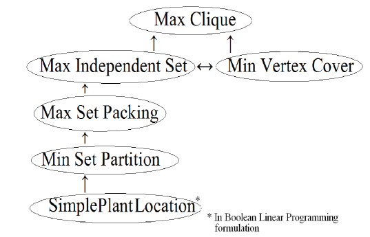
Figure 2: Polynomial-time reductions of optimal recombination problems (all displayed problems are in weighted versions).

The ORP reductions described above are illustrated in Fig. 2.

3.2 Boolean Linear Programming Problems and Hypergraphs

The starting point of all reductions considered above was Theorem 1 which may be viewed as an efficient reduction of the ORP for the Maximum Weight Clique Problem to the Maximum Weight Independent Set Problem in a bipartite graph. In order to generalize this approach now we will move from bipartite graphs to 2-colorable hypergraphs.

A hypergraph $H=(V,E)$ is given by a finite nonempty set of vertices $V$ and a set of edges $E$, where each edge $e\in E$ is a subset of $V$. A subset $S\subseteq V$ is called independent if none of the edges $e\in E$ is a subset of $S$. The Maximum Weight Independent Set Problem on hypergraph $H=(V,E)$ with rational vertex weights $w(v),\ v\in V$ asks for an independent set $S$ with maximum weight $w(S)=\sum_{v\in S}w(v)$.

A generalization of the bipartite graph is the 2-colorable hypergraph: there exists a partition of the vertex set $V$ into two disjoint independent subsets $C_{1}$ and $C_{2}$. The partition $V=C_{1}\cup C_{2}$, $C_{1}\cap C_{2}=\emptyset$ is called a 2-coloring of $H$ and $C_{1},C_{2}$ are the color classes.

Let us denote by $N_{i}$ the set of indices of non-zero elements in constraint $i$ of the Boolean Linear Programming Problem (1)-(3). In the sequel we will assume that at least one of the subsets $N_{i}$ contains two or more elements (otherwise the problem is solved trivially).

Theorem 2

[22] The ORP for Boolean Linear Programming Problem (1)-(3) reduces to the Maximum Weight Independent Set Problem on a 2-colorable hypergraph with a 2-coloring given in the input. Each edge in the 2-colorable hypergraph contains at most $N_{\max}$ vertices, where $N_{\max}=\max_{i=1,\dots,m}|N_{i}|$, and the time complexity of this reduction is $O(m(2^{N_{\max}}+n))$.

Proof. Given an instance of the Boolean Linear Programming Problem with parent solutions $\mbox{\bf p}^{1}$ and $\mbox{\bf p}^{2}$, let us denote $|D(\mbox{\bf p}^{1},\mbox{\bf p}^{2})|$ by $d$ and construct a hypergraph $H$ on $2d$ vertices, assigning each variable $x_{j},\ j\in D(\mbox{\bf p}^{1},\mbox{\bf p}^{2}),$ a couple of vertices $v_{j}$ and $v_{n+j}$. In order to model each of the linear constraints for $i=1,\dots,m$ we will look through all possible combinations of the Boolean variables from $D(\mbox{\bf p}^{1},\mbox{\bf p}^{2})$ involved in this constraint:

$$\{\mbox{\bf x}\in\{0,1\}^{n}:x_{j}=0\ \forall j\not\in N_{i}\cap D(\mbox{\bf p}^{1},\mbox{\bf p}^{2})\}.$$

Let $\mbox{\bf x}^{ik},k=1,\dots,2^{|N_{i}\cap D(\mbox{\bf p}^{1},\mbox{\bf p}^{2})|}$ denote the $k$-th vector in this set. For each combination $k$ which violates a constraint $i$ from (2), i.e.

$$\sum_{j\in N_{i}\cap D(\mbox{\bf p}^{1},\mbox{\bf p}^{2})}a_{ij}x^{ik}_{j}+\sum_{j\in N_{i}\backslash D(\mbox{\bf p}^{1},\mbox{\bf p}^{2})}a_{ij}p^{1}_{j}>b_{i},$$

we add an edge

$$e_{ik}=\{v_{j}:x^{ik}_{j}=1,\ j\in N_{i}\cap D(\mbox{\bf p}^{1},\mbox{\bf p}^{2})\}\cup\{v_{j+n}:x^{ik}_{j}=0,\ j\in N_{i}\cap D(\mbox{\bf p}^{1},\mbox{\bf p}^{2})\}$$

into the hypergraph. (Note that the edge $e_{ik}$ contains at most $|N_{i}|$ elements.) Besides that, we add $d$ edges $\{v_{j},v_{n+j}\},j\in D(p_{1},p_{2})$, to guarantee that both $v_{j}$ and $v_{n+j}$ can not enter into an independent set together.

If x is a feasible solution to the ORP for (1)-(3), then the set of vertices

$$S(\mbox{\bf x})=\{v_{j}:x_{j}=1,j\in D(p_{1},p_{2})\}\cup\{v_{j+n}:x_{j}=0,j\in D(p_{1},p_{2})\}$$

is independent in $H$. Given a set of vertices $S$, we can construct the corresponding vector $\mbox{\bf x}(S)$, assigning $\mbox{\bf x}(S)_{j}=1$ if $v_{j}\in S,$ $j\in D(\mbox{\bf p}^{1},\mbox{\bf p}^{2})$ or if $p^{1}_{j}=p^{2}_{j}=1$. Otherwise $\mbox{\bf x}(S)_{j}=0.$ Then for each independent set $S$ of $d$ vertices, $\mbox{\bf x}(S)$ is feasible in the Boolean Linear Programming Problem.

The hypergraph vertices are given the following weights:

$$w(v_{j})=c_{j}+\lambda,\ w(v_{n+j})=\lambda,\ {j\in D(\mbox{\bf p}^{1},\mbox{\bf p}^{2}),}$$

where $\lambda>2\sum_{j\in D(p_{1},p_{2})}|c_{j}|$.

Now each maximum weight independent set $S^{*}$ contains either $v_{j}$ or $v_{n+j}$ for any ${j\in D(\mbox{\bf p}^{1},\mbox{\bf p}^{2})}$. Indeed, there must exist a feasible solution to the ORP and it corresponds to an independent set of weight at least $\lambda d$. However, if an independent set neither contains $v_{j}$ nor $v_{n+j}$ then its weight is below $\lambda d-\lambda/2$.

So, optimal independent set $S^{*}$ corresponds to a feasible vector $\mbox{\bf x}(S^{*})$ with the goal function value

$${\bf cx}(S^{*})=\sum_{j\in S^{*},\ j\leq n}c_{j}+\sum_{j\not\in D(\mbox{\bf p}^{1},\mbox{\bf p}^{2})}c_{j}p^{1}_{j}=w(S^{*})-\lambda d+\sum_{j\not\in D(\mbox{\bf p}^{1},\mbox{\bf p}^{2})}c_{j}p^{1}_{j}.$$

Under the mapping $S(\mbox{\bf x})$, which is inverse to $\mbox{\bf x}(S)$, any feasible vector x yields an independent set of weight

$$w(S(\mbox{\bf x}))={\bf cx}+\lambda d-\sum_{j\not\in D(\mbox{\bf p}^{1},\mbox{\bf p}^{2})}c_{j}p^{1}_{j},$$

therefore $\mbox{\bf x}(S^{*})$ is an optimal solution to the ORP. $\Box$

Note that if an edge $e\in H$ consists of a single vertex, $e=\{v\}$, then the vertex $v$ can not enter into the independent sets. All of such vertices should be excluded from the hypergraph $H$ constructed in Theorem 2. Let us denote the resulting hypergraph by $H^{\prime}$. If $N_{\max}\leq 2$, then the hypergraph $H^{\prime}$ is an ordinary graph with at most $2d$ vertices. Thus, by Theorem 2 the ORP reduces to the Maximum Weight Independent Set Problem in a bipartite graph $H^{\prime}$, which is solvable in $O(d^{3})$ operations. Using this fact, Theorem 1 may be extended as follows:

Corollary 3

[22] The ORP for Linear Boolean Programming Problem with at most two variables per inequality is solvable in time $O(|D(\mbox{\bf p}^{1},\mbox{\bf p}^{2})|^{3}+mn)$, if the solutions are represented by vectors $x\in\{0,1\}^{n}$.

The class of Linear Boolean Programming Problems with at most two variables per inequality includes the Vertex Cover Problem and the Minimum 2-Satisfiability Problem – see e.g [30].

4 NP-hard Optimal Recombination Problems in Boolean Linear Programming

It was shown above that the optimal recombination on the class of Boolean Linear Programming Problems is related to the Maximum Weight Independent Set Problem on hypergraphs with a given 2-coloring. The next lemma indicates that in general case the latter problem is NP-hard.

Lemma 1

[22] The problem of finding a maximum size independent set in a hypergraph with all edges of size 3 is strongly NP-hard even if a 2-coloring is given.

Proof. Let us construct a reduction from the strongly NP-hard Maximum Size Independent Set Problem on ordinary graphs to the problem under consideration. Given a graph $G=(V,E)$ with the set of vertices $V=\{v_{1},\dots,v_{n}\}$, consider a hypergraph $H=(V^{\prime},E^{\prime})$ on the set of vertices $V^{\prime}=\{v_{1},\dots,v_{2n}\}$, where for each edge $e=\{v_{i},v_{j}\}\in E$ there are $n$ edges of the form $\{v_{i},v_{j},v_{n+k}\},\ k=1,\dots,n$ in $E^{\prime}$. A 2-coloring for this hypergraph can be composed of color classes $C_{1}=V$ and $C_{2}=\{v_{n+1},\dots,v_{2n}\}$. Any maximum size independent set in this hypergraph consists of the set of vertices $\{v_{n+1},\dots,v_{2n}\}$ joined with a maximum size independent set $S^{*}$ in $G$. Therefore, any maximum size independent set in $H$ immediately induces a maximum size independent set for $G$. $\Box$

The Maximum Size Independent Set Problem in a hypergraph $H=(V,E)$ may be formulated as a Boolean Linear Programming Problem

$$\max\left\{\mbox{$\sum_{j=1}^{n}x_{j}$}:{\bf Ax}\leq{\bf b},\mbox{\bf x}\in\{0,1\}^{n}\right\}$$ (20)

with $m=|E|,n=|V|,$ $b_{i}=|e_{i}|-1,\ i=1,\dots,m$ and $a_{ij}=1$ iff $v_{j}\in e_{i}$, otherwise $a_{ij}=0$. In the special case where $H$ is 2-colorable, we can take $\mbox{\bf p}^{1}$ and $\mbox{\bf p}^{2}$ as the indicator vectors for the color classes $C_{1}$ and $C_{2}$ of any 2-coloring. Then $D(\mbox{\bf p}^{1},\mbox{\bf p}^{2})=\{1,\dots,n\}$ and the ORP for the Boolean Linear Programming Problem (20) becomes equivalent to solving the maximum size independent set in a hypergraph $H$ with a given 2-coloring. In view of Lemma 1, this leads to the following

Theorem 3

[22] The optimal recombination problem for Boolean Linear Programming Problem is strongly NP-hard even in the case where $|N_{i}|=3$ for all $i=1,\dots,m$; $c_{j}=1$ for all $j=1,\dots,n$ and matrix ${\bf A}$ is Boolean.

In the rest of this section we will discuss NP-hardness of the ORPs for some well-known Boolean Linear Programming Problems.

4.1 One-Dimensional Knapsack and Bin Packing

In Boolean linear programming formulation the One-Dimensional Knapsack Problem has the following formulation

$$\max\left\{{\bf cx}:{\bf a}\mbox{\bf x}\leq A,\mbox{\bf x}\in\{0,1\}^{n}\right\},$$ (21)

where ${\bf c}=(c_{1},\dots,c_{n})$, ${\bf a}=(a_{1},\dots,a_{n})$, $a_{j}\geq 0,c_{j}\geq 0,j=1,\dots,n,$ and $A\geq 0$ are integer.

Below we also consider the One-Dimensional Bin Packing Problem. Given an integer number $A$ (size of a bin) and $k$ integer numbers $a_{1},\dots,a_{k}$ (sizes of items), $a_{i}\leq A,\ i=1,\dots,k$ it is required to locate the items into the minimal number of bins, so that the sum of sizes of items in each bin does not exceed $A$.

The One-Dimensional Bin Packing Problem may be formulated as a Boolean Linear Programming Problem the following way (a more "standard" integer linear programming formulation can be found e.g. in [35]). Let a Boolean variable $y_{j}$ be the indicator of usage of a bin $j,\ j=1,\dots,k$ and a Boolean variable $x_{ij}$ be the indicator of packing item $i$ in bin $j$, $i,j=1,\dots,k$. Find

$$\mbox{min}\sum_{j=1}^{k}y_{j}$$ (22)

s. t.

$$\sum_{j=1}^{k}x_{ij}=1,\ \ i=1,\dots,k,$$ (23)

$$\sum_{i=1}^{k}a_{i}x_{ij}\leq A,\ \ j=1,2,\dots,k,$$ (24)

$$y_{j}\geq x_{ij},\ \ i=1,\dots,k,\ j=1,\dots,k,$$ (25)

$$x_{ij},\ y_{j}\in\{0,1\},\ \ i=1,\dots,k,\ j=1,2,\dots,k.$$ (26)

Note that for solutions encoding it suffices to store only the matrix of assignments $(x_{ij})$, since the vector $(y_{1},\dots,y_{k})$ corresponding to such a matrix is uniquely defined. Below we assume that $(k\times k)$-matrices of assignments are used to encode the feasible solutions and $n=k^{2}$.

The following special case of the well-known Partition Problem [26] will be called Bounded Partition: Given $2m$ positive integer numbers $\alpha_{1},\ldots,\alpha_{2m}$, which satisfy

$$\frac{B}{m+1}<\alpha_{j}<\frac{B}{m-1},\ \ j=1,\dots,2m,$$ (27)

where $B=\sum_{j=1}^{2m}\alpha_{j}/2$, is there a vector $\mbox{\bf x}\in\{0,1\}^{2m}$, such that

$$\sum_{j=1}^{2m}\alpha_{j}x_{j}=B?$$ (28)

The next lemma is due to P. Schuurman and G. Woeginger.

Lemma 2

[47] The Bounded Partition Problem is NP-complete.

Proof. NP-completeness of this problem may be established via reduction from the following NP-complete modification of Partition Problem [26]: given a set of $2m$ positive integers $\alpha^{\prime}_{j},\ j=1,\dots,2m$, it is required to recognize existence of such $\mbox{\bf x}\in\{0,1\}^{2m}$, that

$$\sum_{j=1}^{2m}x_{j}=m\ \ \mbox{and}\ \ \sum_{j=1}^{2m}\alpha^{\prime}_{j}x_{j}=\frac{1}{2}\sum_{j=1}^{2m}\alpha^{\prime}_{j}.$$ (29)

The reduction consists in setting $\alpha_{i}=\alpha^{\prime}_{i}+M,\ i=1,\dots,2m,$ with a sufficiently large integer $M$, e.g., $M=2m\cdot\max\{\alpha^{\prime}_{j}:j=1,\dots,2m\}$. Satisfaction of (27), as well as equivalence of (29) and (28), given this set of parameters $\{\alpha_{i}\}$, is verified straightforwardly. $\Box$

Theorem 4

[18] The ORPs for the One-Dimensional Knapsack Problem (21) and the One-Dimensional Bin-Packing Problem (22) – (26) are NP-hard.

Proof. 1. Consider ORP for Knapsack Problem (21). The NP-hardness of this problem can be established using a polynomial-time Turing reduction of Bounded Partition Problem to it. W. l. o. g. let us assume $m>2$.

Note that if an instance of Bounded Partition Problem has the answer "yes", then there exists a vector $\mbox{\bf x}^{\prime}\in\{0,1\}^{2m}$, such that $\sum_{i=1}^{2m}\alpha_{i}x^{\prime}_{i}=B$, and since $B/(m+1)<\alpha_{i}<B/(m-1),\ i=1,\dots,2m$, this vector contains exactly $m$ ones, which is less than ${2m-2}$ because $m>2$. On the contrary, if the instance of Partition Problem has the answer "no", then such a vector does not exist.

The Turing reduction of Bounded Partition Problem to the ORP for One-Dimensional Knapsack problem is based on enumeration of polynomial number of different pairs of parent solutions (and the corresponding ORP instances). Assume $n=2m,$ $A=B$ and ${c_{j}=a_{j}=\alpha_{j}},\ j=1,\dots,n,$ and enumerate all of the $2m\choose 2$ pairs of variables with indices $\{i_{\ell},j_{\ell}\},\ {\ell}=1,\dots,{2m\choose 2}$. For each pair $i_{\ell},j_{\ell}$ we set $p^{1}_{i_{\ell}}=p^{2}_{j_{\ell}}=0$ and fill the remaining positions $j\not\in\{i_{\ell},j_{\ell}\}$ so that $p^{1}_{j}+p^{2}_{j}=1$ and each of the parent solutions contains in total $m-1$ ones (such parent solutions will be feasible since $a_{j}<A/(m-1),\ j=1,\dots,n$). The greatest value among the optima of the constructed ORPs equals $A$ iff the answer to the instance of Partition Problem is "yes". This implies NP-hardness of the ORP for One-Dimensional Knapsack Problem.

2. The proof of NP-hardness of the ORP for One-Dimensional Bin-Packing Problem is based on a similar (but more time demanding) Turing reduction from Bounded Partition Problem. Now we assume $k=2m,$ $A=B$, and ${a_{i}=\alpha_{i}},\ i=1,\dots,k$. In what follows it is supposed that $m>4$.

Given an instance of Bounded Partition Problem, we enumerate a polynomial number of parent solutions, choosing them in such a way that (i) $2m-4$ items in the offspring solution are packed into the first two containers, (ii) among them, a pair of "selected" items may be packed only in bin 2, (iii) four other "selected" items may be packed either in bin 1 or in bin 3 optionally. Let us describe this reduction in detail.

As in the first part of the proof we enumerate all of the $2m\choose 2$ pairs of items $\{i_{\ell},i^{\prime}_{\ell}\},\ {\ell}=1,\dots,{2m\choose 2},$ aiming to fix the corresponding variables $\{x_{i_{\ell},1},x_{i^{\prime}_{\ell},1}\}$ to zero value.

For each of the pairs $\{i_{\ell},i^{\prime}_{\ell}\}$ enumerate all $2m-2\choose 2$ pairs $\{u_{r},u^{\prime}_{r}\},\ {r}=1,\dots,{2m-2\choose 2}$ drawn from the rest of the items. Given $\{i_{\ell},i^{\prime}_{\ell}\}$ and $\{u_{r},u^{\prime}_{r}\}$, enumerate all $2m-4\choose 2$ pairs $\{v_{s},v^{\prime}_{s}\},\ {s}=1,\dots,{2m-4\choose 2},$ in the rest of the items.

To ensure that for given $\ell,r$ and $s$, the items $\{i_{\ell},i^{\prime}_{\ell}\}$ in the offspring solution are packed in bin 2, while items $u_{r},u^{\prime}_{r},v_{s},v^{\prime}_{s}$ may be packed only in bin 1 or bin 3, the pair of parent solutions ${\bf p}^{1}=(p^{1}_{ij})$ and ${\bf p}^{2}=(p^{2}_{ij})$ is defined the following way.

In the first column of parent solutions

$$p^{1}_{i_{\ell},1}=p^{1}_{i^{\prime}_{\ell},1}=p^{2}_{i_{\ell},1}=p^{2}_{i^{\prime}_{\ell},1}=0,$$

$$p^{1}_{u_{r},1}=p^{1}_{u^{\prime}_{r},1}=1,\ p^{2}_{u_{r},1}=p^{2}_{u^{\prime}_{r},1}=0,$$

$$p^{1}_{v_{s},1}=p^{1}_{v^{\prime}_{s},1}=0,\ p^{2}_{v_{s},1}=p^{2}_{v^{\prime}_{s},1}=1$$

and fill the remaining positions $i\not\in\{i_{\ell},i^{\prime}_{\ell},u_{r},u^{\prime}_{r},v_{s},v^{\prime}_{s}\}$ so that $p^{1}_{i,1}+p^{2}_{i,1}=1$ holds and each of the parent solutions has $m-1$ ones in column 1. These parent solutions satisfy condition (24) for bin $j=1$, since ${a_{i}<A/(m-1),}\ i=1,\dots,k$.

Let the second column in each of the parent solutions be identical to the first column of the other parent, except for the components corresponding to the six items mentioned above. Two entries 1 in rows $v_{s}$ and $v^{\prime}_{s}$ of the parent solution ${\bf p}^{1}$ are placed into column $j=3$, rather than column $j=2$. Two entries 1 in rows $u_{r}$ and $u^{\prime}_{r}$ of the parent solution ${\bf p}^{2}$ are placed into column $j=3$, rather than column $j=2$. Besides that, in column $j=2$ of both parent solutions the entries 1 are placed in rows $i_{\ell}$ and $i^{\prime}_{\ell}$.

In each parent solution the second column contains $m-1$ entries 1, thus condition (24) for bin $j=2$ is satisfied as well as in the case of $j=1$. For bin $j=3$ this condition holds, since ${a_{i}<A/4,}\ i=1,\dots,k$ when $m>4$. Note that all feasible solutions to the ORP corresponding to a triple of indices $\ell,r,s$ contain the items $i_{\ell},i^{\prime}_{\ell}$ in the second bin, while items $u_{r}$, $u^{\prime}_{r}$, $v_{s}$ and $v^{\prime}_{s}$ may appear either in bin 1 or in bin 3.

If an instance of Bounded Partition Problem has the answer "yes" then at least one of the constructed ORPs has the optimum objective function value $2$. Indeed, in such a case the vector $\mbox{\bf x}^{\prime}$ that satisfies condition (28) should have two entries $x^{\prime}_{\hat{i}}=x^{\prime}_{\bar{i}}=0$ for some $\hat{i},\bar{i}$. Besides that, there are four indices $\hat{u},\bar{u},\hat{v}$ and $\bar{v}$, such that $x^{\prime}_{\hat{u}}=x^{\prime}_{\bar{u}}=x^{\prime}_{\hat{v}}=x^{\prime}_{\bar{v}}=1$, since this vector contains not less than $m$ entries 1. The corresponding ORP with $\{i_{\ell},i^{\prime}_{\ell}\}=\{\hat{i},\bar{i}\}$, $\{u_{r},u^{\prime}_{r}\}=\{\hat{u},\bar{u}\}$ and $\{v_{s},v^{\prime}_{s}\}=\{\hat{v},\bar{v}\}$ has a feasible solution $(x^{\prime}_{ij})$, where the first column is identical to $\mbox{\bf x}^{\prime}$, the entries of the second column are $x^{\prime}_{i2}=1-x^{\prime}_{i},\ i=1,\dots,k$, and the rest of the columns are filled with zeros.

Conversely, if an optimal solution $x^{*}_{ij}$ to one of the constructed ORPs has the value 2, then setting $x_{i}=x^{*}_{i1},\ i=1,\dots,k,$ we obtain equality (28). $\Box$

The One-Dimensional Bin Packing problem is contained as a special case in a number of packing and scheduling problems, so the latter theorem may be applicable in analysis of complexity of the ORPs for these problems. In particular, Theorem 4 implies NP-hardness of the ORP for the Transfer Line Balancing Problem [19].

4.2 Set Covering and Location Problems

The next example of an NP-hard ORP is that for the Set Covering Problem, which may be considered as a special case of (1)-(3):

$$\min\left\{{\bf cx}:{\bf Ax}\geq{\bf e},\ \mbox{\bf x}\in\{0,1\}^{n}\right\},$$ (30)

where ${\bf A}$ is a Boolean $(m\times n)$-matrix; ${\bf c}=(c_{1},\dots,c_{n});$ $c_{j}\geq 0,\ j=1,\dots,n$. Let us assume the binary representation of solutions by the vector x. Given an instance of the Set Covering Problem, one may construct a new instance with a doubled set of columns in the matrix ${\bf A}^{\prime}=({\bf AA})$ and a doubled vector ${\bf c}^{\prime}={(c_{1},\dots,c_{n},c_{1},\dots,c_{n})}$. Then an instance of the NP-hard Set Covering Problem (30) is equivalent to the ORP for the modified set covering instance where the input consists of $(m\times 2n)$-matrix ${\bf A}^{\prime}$, $2n$-vector ${\bf c}^{\prime}$ and the feasible parent solutions $\mbox{\bf p}^{1},\mbox{\bf p}^{2},$ with $p^{1}_{j}=1,p^{2}_{j}=0$ for $j=1,\dots,n$ and $p^{1}_{j}=0,p^{2}_{j}=1$ for $j=n+1,\dots,2n$. So, the ORP for the Set Covering Problem is also NP-hard.

Interestingly, in some cases the ORP may be even harder than the original problem (assuming P$\neq$ NP). This can be illustrated on the example of the Set Covering Problem. A special case of this problem, defined by the restriction $a_{i,1}=1,i=1,\dots,m;\ c_{1}=0$ is trivially solvable: $\mbox{\bf x}=(1,0,0,\dots,0)$ is the optimal solution. However, in the case $p^{1}_{1}=p^{2}_{1}=0$, the ORP becomes NP-hard under this restriction.

The Set Covering Problem may be efficiently transformed to the Simple Plant Location Problem (10)-(11) – see e.g. transformation T3  in [38]. In this case the dimensions $m$ and $n$ in both problems are equal, $C_{i}=c_{i}$ for $i=1,\dots,n$ and

$$c_{ij}=\left\{\begin{array}[]{cl}\sum_{k=1}^{n}c_{k}+1,&\mbox{ if }\ a_{ij}=0,\\ 0,&\mbox{ if }\ a_{ij}=1,\end{array}\right.\ \ \mbox{for all}\ \ i=1,\dots,n,\ j=1,\dots,m.$$

It is easy to verify that a vector ${\bf x}^{*}$ in the optimal solution to this instance of the Simple Plant Location Problem will be an optimal set covering solution as well. Thus, if the solution representation in the Simple Plant Location Problem is given only by the vector $\bf x$, then this reduction meets the conditions of Proposition 2. The subset of solutions to the Simple Plant Location Problem $\beta({\rm Sol}_{1}(I))$ is characterized in this case by the threshold on objective function $f_{\rm splp}({\bf y})<\sum_{j=1}^{n}c_{j}+1$, which ensures that all constraints of the Set Covering Problem are met. Therefore, an NP-hard ORP problem is efficiently reduced to the ORP for (10)-(11) and the following proposition holds.

Proposition 3

[22] The ORP for the Simple Plant Location Problem (10), (11) is NP-hard.

The well-known $p$-Median Problem may be defined as a modification of the Simple Plant Location Problem (10), (11): it suffices to assume $C_{k}=0,\ j=1,\dots,n,$ and to substitude the inequality (11) by constraint

$$\sum_{i=1}^{n}x_{i}=p,$$ (31)

where $1\leq p\leq n$ is a parameter given in the problem input.

Proposition 4

[22] The ORP for the $p$-Median Problem (10), (31) is NP-hard.

Proof. E. Alexeeva, Yu. Kochetov and A. Plyasunov in [4] propose a reduction of an NP-hard Graph Partitioning Problem to the $p$-Median Problem with $n=|V|$ and $p=|V|/2$, where $V$ is the set of the graph vertices and $|V|$ is even. Thus, this special case of the $p$-Median Problem is NP-hard as well. Consider an ORP for this case of the $p$-Median Problem with parent solutions $\mbox{\bf p}^{1}=(1,\dots,1,0,\dots,0)$ and $\mbox{\bf p}^{2}=(0,\dots,0,1,\dots,1)$ of $n/2$ ones. Obviously, such ORP is equivalent to the original $p$-Median Problem.  $\Box$

5 Travelling Salesman Problem

In this section we consider the Travelling Salesman Problem (TSP): suppose a digraph $G$ without loops or multiple arcs is given. The set of vertices of $G$ is $V$ and a set of arcs is $A$. A weight (length) $c_{ij}\geq 0$ of each arc $(i,j)\in A$ is given as well. It is required to find a Hamiltonian circuit of minimum length.

If for each arc $(i,j)\in A$ there exists a reverse one ${(j,i)\in A}$ and $c_{ij}=c_{ji}$, then the TSP is called symmetric and $G$ is assumed to be an ordinary graph. Without this assumption we will call the problem the general case of TSP.

Feasible solution to the TSP may be encoded as a sequence of the vertex numbers in the TSP tour, or as a permutation matrix where the element in row $i$ and column $j$ equals one iff the vertex $j$ immediately follows the vertex $i$ in the TSP tour. (For the sake of consistency with Definition 1 one may assume that the elements of the matrix are written sequentially in a string $\mbox{\bf x}\in\mbox{\rm Sol}$.)

Unfortunately there are $|V|$ different sequences of vertices encoding the same Hamiltonian circuit. The second encoding has an advantage that a Hamiltonian circuit is uniquely represented by a permutation matrix. Therefore in what follows we assume the second encoding. If this encoding is used in the symmetric case, it is sufficient to define only the elements above the diagonal of the matrix, so the rest of the elements are dismissed from subsequent consideration in the symmetric case.

The encoding by permutation matrix defines an ORP that consists in finding a shortest travelling salesman’s tour which coincides with two given feasible parent solutions in those arcs (or edges) which belong to both parent tours and does not contain the arcs (or edges) which are absent in both parent solutions.

5.1 Symmetric Case

In [33] it is proven that recognition of Hamiltonian grid graphs (the Hamilton Cycle Problem) is NP-complete. Recall that a graph $G^{\prime}=(V^{\prime},E^{\prime})$ with vertex set $V^{\prime}$ and edge set $E^{\prime}$ is called a grid graph, if its vertices are the integer vectors $v=(x_{v},y_{v})\in{\bf Z}^{2}$ on plane, i.e., $V^{\prime}\subset{\bf Z}^{2}$, and a pair of vertices is connected by an edge iff the Euclidean distance between them is equal to 1. Here and below, $\bf Z$ denotes the set of integer numbers. Let us call the edges that connect two vertices in ${\bf Z}^{2}$ with equal first coordinates vertical edges. The edges that connect two vertices in ${\bf Z}^{2}$ with equal second coordinates will be called horizontal edges.

Let us assume that $V^{\prime}>4$, graph $G^{\prime}$ is connected and there are no bridges in $G^{\prime}$ (note that if any of these assumptions is violated, then existence of a Hamiltonian cycle in $G^{\prime}$ can be recognized in polynomial time). Now we will construct a reduction from the Hamilton Cycle Problem for $G^{\prime}$ to an ORP for a complete edge-weighted graph $G=(V,E)$, where $V=V^{\prime}$.

Let the edge weights $c_{ij}$ in $G$ be defined so that if a pair of vertices $\{v_{i},v_{j}\}$ is connected by an edge of $G^{\prime}$, then $c_{ij}=0$; all other edges in $G$ have the weight 1. Consider the following two parent solutions of the TSP on graph $G$ (an example of graph $G^{\prime}$ and two parent solutions for the corresponding TSP is given in Fig. 3).

Figure 3: Example of two parent tours used in reduction from Hamilton Cycle Problem to ORP in symmetric case.

Let $y_{\min}=\min_{v\in V^{\prime}}y_{v},\ y_{\max}=\max_{v\in V^{\prime}}y_{v}.$ For any integer $y\in\{y_{\min},\dots,$ $y_{\max}\}$, the horizontal chain that passes through vertices $v\in V^{\prime}$ with $y_{v}=y$ by increasing values of coordinate $x$ is denoted by $P^{y}$. Let the first parent tour follow the chains $P^{y_{\min}},P^{y_{\min}+1},\dots,P^{y_{\max}}$, connecting the right-hand end of each chain $P^{y}$ with $y<y_{\max}$ to the left-hand end of the chain $P^{y+1}$. Note that these connections never coincide with vertical edges because $G^{\prime}$ has no bridges. To create a cycle, connect the right-hand end $v_{\rm TR}$ of the chain $P^{y_{\max}}$ to the left-hand end $v_{\rm BL}$ of the chain $P^{y_{\min}}$.

The second parent tour is constructed similarly using the vertical chains. Let $x_{\min}=\min_{v\in V^{\prime}}x_{v}$, $x_{\max}=\max_{v\in V^{\prime}}x_{v}$. For any integer $x\in\{x_{\min},\dots,x_{\max}\},$ the vertical chain that passes monotonically in $y$ through the vertices $v\in V^{\prime}$, such that $x_{v}=x$, is denoted by $Q^{x}$. The second parent tour follows the chains $Q^{x_{\min}},Q^{x_{\min}+1},\dots,Q^{x_{\max}}$, connecting the lower end of each chain $Q^{x}$ with $x<x_{\max}$ to the upper end of chain $Q^{x+1}$. These connections never coincide with horizontal edges since $G^{\prime}$ has no bridges. Finally, the lower end $v_{\rm RB}$ of chain $Q^{x_{\max}}$ is connected to the upper end $v_{\rm LT}$ of chain $Q^{x_{\min}}$.

Note that the constructed parent tours have no common edges. Indeed, common slanting edges do not exist since $V^{\prime}>4$. The horizontal edges belong to the first tour only, except for the situation where $y_{v_{\rm RB}}=y_{v_{\rm LT}}$ and the edge $\{v_{\rm RB},v_{\rm LT}\}$ of the second tour is oriented horizontally. But if the first parent tour included the edge $\{v_{\rm RB},v_{\rm LT}\}$ in this situation, then the edge $\{v_{\rm RB},v_{\rm LT}\}$ would be a bridge in graph $G^{\prime}$. Therefore the parent tours can not have the common horizontal edges. Similarly the vertical edges belong to the second tour only, except for the case where $x_{v_{\rm TR}}=x_{v_{\rm BL}}$ and the edge $\{v_{\rm TR},v_{\rm BL}\}$ of the first tour is oriented vertically. But in this case the parent tour can not contain the edge $\{v_{\rm TR},v_{\rm BL}\}$, since $G^{\prime}$ has no bridges.

Note also that the union of edges of parent solutions contains $E^{\prime}$. Consequently, any Hamiltonian cycle in graph $G^{\prime}$ is a feasible solution of the ORP. At the same time, a feasible solution of the ORP has zero value of objective function iff it contains only the edges of $E^{\prime}$. Therefore, the optimal value of objective function in the ORP under consideration is equal to 0 iff there exists a Hamiltonian cycle in graph $G^{\prime}$. So, the following theorem is proven.

Theorem 5

[23] Optimal recombination for the TSP in the symmetric case is strongly NP-hard.

In [33] it is also proven that recognition of grid graphs with a Hamiltonian path is NP-complete. Optimal recombination for this problem consists in finding a shortest Hamiltonian path, which uses those edges where both parent tours coincide, and does not use the edges absent in both parent tours. The following theorem is proved analogously to Theorem 5.

Theorem 6

[23] Optimal recombination for the problem of finding the shortest Hamiltonian path in a graph with arbitrary edge lengths is strongly NP-hard.

Note that in the proof of Theorem 6, unlike in Theorem 5, it is impossible simply to exclude the cases where graph $G^{\prime}$ has bridges. Instead, the reduction should treat separately each maximal (by inclusion) subgraph without bridges.

Many scheduling problems with setup times contain the problem of finding the shortest Hamiltonian path in a digraph as a special case. In this case the vertices correspond to jobs, the arcs correspond to setups and the arc lengths define the setup times. In view of numerous applications of scheduling problems with setup times, in Section 6 the problem of finding the shortest Hamiltonian path in a digraph is treated as a scheduling problem.

5.2 The General Case

In the general case of TSP the ORP is not a more general problem than the ORP considered in Subsection 5.1 because in the problem input we have two directed parent paths, while in the symmetric case the parent paths were undirected. Even if the distance matrix $(c_{ij})$ is symmetric, a pair of directed parent tours defines a significantly different set of feasible solutions, compared to the undirected case. Therefore, the general case requires a separate consideration of ORP complexity.

Theorem 7

[23] Optimal recombination for the TSP in the general case is strongly NP-hard.

Proof. We use a modification of the textbook reduction of the Vertex Cover Problem to the TSP [26].

Suppose an instance of a Vertex Cover Problem is given as a graph $G^{\prime}=(V^{\prime},E^{\prime})$. It is required to find a vertex cover of minimal size in $G^{\prime}$. Let us assume that the vertices in $V^{\prime}$ are enumerated, i.e. $V^{\prime}=\{v_{1},\dots,v_{n}\}$, where $n=|V^{\prime}|$, and let $m=|E^{\prime}|$.

Consider a complete digraph $G=(V,A)$ where the set of vertices $V$ consists of $|E^{\prime}|$ cover-testing components, each one containing 12 vertices: $V_{e}=\{(v_{i},e,k),(v_{j},e,k):1\leq k\leq 6\}$ for each $e=\{v_{i},v_{j}\}\in E^{\prime},\ i<j$. Besides that, $V$ contains $n$ selector vertices denoted by $a_{1},\dots,a_{n}$, and a supplementary vertex $a_{n+1}$.

Let the parent tours in graph $G$ be the two circuits defined below (an example of a pair of such circuits for the case of $G^{\prime}=K_{3}$ is provided in Fig. 4).

Figure 4: A pair of parent circuits for the case of $G^{\prime}=K_{3}$. It is supposed that the incident edges are enumerated as follows. For vertex $v^{1}:\ e^{v_{1},1}=e_{1},\ e^{v_{1},2}=e_{3};$ for vertex $v^{2}:\ e^{v_{2},1}=e_{1},\ e^{v_{2},2}=e_{2};$ for vertex $v^{3}:\ e^{v_{3},1}=e_{2},e^{v_{3},2}=e_{3}$.

1. Each cover-testing component $V_{e}$, where $e=\{v_{i},v_{j}\}\in E^{\prime}$ and $i<j$ is visited twice by the first tour. The first time it visits the vertices that correspond to $v_{i}$ in the sequence

$$(v_{i},e,1),\dots,(v_{i},e,6),$$ (32)

the second time it visits the vertices corresponding to $v_{j}$, in the sequence

$$(v_{j},e,1),\dots,(v_{j},e,6).$$ (33)

2. The second tour goes through each cover-testing component $V_{e}$, where $e=\{v_{i},v_{j}\}\in E^{\prime}$ and $i<j$ in the following sequence:

$$(v_{i},e,2),(v_{i},e,3),(v_{j},e,1),(v_{j},e,2),(v_{j},e,3),(v_{i},e,1),$$

$$(v_{i},e,6),(v_{j},e,4),(v_{j},e,5),(v_{j},e,6),(v_{i},e,4),(v_{i},e,5).$$

The first parent tour connects the cover-testing components as follows. For each vertex $v\in V^{\prime}$ order arbitrarily the edges incident to $v$ in graph $G^{\prime}$ in sequence: $e^{v,1},e^{v,2},\dots,e^{v,deg(v)},$ where $deg(v)$ is the degree of vertex $v$ in $G^{\prime}$. In the cover-testing components, following the chosen sequence $e^{v,1},e^{v,2},\dots,e^{v,deg(v)}$, this tour passes 6 vertices in each of the components $(v,e,k),\ k=1,\dots,6,\ e\in\{e^{v,1},e^{v,2},\dots,e^{v,deg(v)}\}$. Thus, each vertex of any cover-testing component $V_{e}$, $e=\{u,v\}\in E^{\prime}$ will be visited by one of the two 6-vertex sub-tours.

The second tour passes the cover-testing components in an arbitrary order of edges $V_{e_{1}},\dots,V_{e_{m}}$, entering each component $V_{e_{k}}$ for any $e_{k}=\{v_{i_{k}},v_{j_{k}}\}\in E^{\prime},\ i_{k}<j_{k},\ k=1,\dots,m,$ via vertex $(v_{i_{k}},e_{k},2)$ and exiting through vertex $(v_{i_{k}},e_{k},5)$. Thus, a sequence of vertex indices $i_{1},\dots,i_{m}$ is induced (repetitions are possible). In what follows, we will need the beginning $i_{1}$ and the end $i_{m}$ of this sequence.

The parent sub-tours described above are connected to form two Hamiltonian circuits in $G$ using the vertices $a_{1},\dots,a_{n+1}$. The first circuit is completed using the arcs

$$\Big{(}a_{1},(v_{1},e^{v_{1},1},1)\Big{)},\ \Big{(}(v_{1},e^{v_{1},deg(v_{1})},6),a_{2}\Big{)},\$$

$$\Big{(}a_{2},(v_{2},e^{v_{2},1},1)\Big{)},\ \Big{(}(v_{2},e^{v_{2},deg(v_{2})},6),a_{3}\Big{)},$$

$$\dots,$$

$$\Big{(}a_{n},(v_{n},e^{v_{n},1},1)\Big{)},\ \Big{(}(v_{n},e^{v_{n},deg(v_{n})},6),a_{n+1}\Big{)},\Big{(}a_{n+1},a_{1}\Big{)}.$$

The second circuit is completed by the arcs

$$\Big{(}a_{1},a_{2}\Big{)},\dots,\Big{(}a_{n-1},a_{n}\Big{)},\Big{(}a_{n},a_{n+1}\Big{)},$$

$$\Big{(}a_{n+1},(v_{i_{1}},e_{1},2)\Big{)},\ \Big{(}(v_{i_{m}},e_{m},5),a_{1}\Big{)}.$$

Assign unit weights to all arcs $\Big{(}a_{i},(v_{i},e^{v_{i},1},1)\Big{)},\ i=1,\dots,n$ in the complete digraph $G$. Besides that, assign weight $n+1$ to all arcs of the second tour which are connecting the components $V_{e_{1}},\dots,V_{e_{m}}$, the same weights are assigned to the arcs $\Big{(}a_{n+1},(v_{i_{1}},e_{1},2)\Big{)}$ and $\Big{(}(v_{i_{m}},e_{m},5),a_{1}\Big{)}$. All other arcs in $G$ are given weight 0.

Note that for any vertex cover $C$ of graph $G^{\prime}$, the set of feasible solutions of ORP with two parents defined above contains a circuit $R(C)$ with the following structure (see an example of such a circuit for the case of $G^{\prime}=K_{3}$ in Fig. 5).

For each $v_{i}\in C$ the circuit $R(C)$ contains the arcs $\Big{(}a_{i},(v_{i},e^{v_{i},1},1)\Big{)}$ and $\Big{(}(v_{i},e^{v_{i},deg(v_{i})},6),a_{i+1}\Big{)}$. The components $V_{e},\ e\in\{e^{v_{i},1},e^{v_{i},2},\dots,e^{v_{i},deg(v_{i})}\}$ are connected together by the arcs from the first tour. For each vertex $v_{i}$ which does not belong to $C$, the circuit $R(C)$ has an arc $(a_{i},a_{i+1})$. Also, $R(C)$ passes the arc $(a_{n+1},a_{1})$.

The circuit $R(C)$ visits each cover-testing component $V_{e}$ by one of the two ways:

1. If both endpoints of an edge $e$ belong to $C$, then $R(C)$ passes the component following the same arcs as the first parent tour.

2. If $e=\{u,v\}$, $u\in C$, $v\not\in C$, then $R(C)$ visits the vertices of the component in sequence

$$(u,e,1),(u,e,2),(u,e,3),\ \ (v,e,1),\dots,(v,e,6),\ \ (u,e,4),(u,e,5),(u,e,6).$$

One can check straightforwardly that this sequence does not violate the ORP constraints.

Figure 5: An ORP solution $R(C)$ corresponding to the vertex cover $\{v_{1},v_{3}\}$ of graph $G^{\prime}=K_{3}$.

In general, the circuit $R(C)$ is a feasible solution to the ORP because, on one hand, all arcs used in $R(C)$ are present at least in one of the parent tours. On the other hand, both parent tours contain only the arcs of the type

$$\Big{(}(u,e,2),(u,e,3)\Big{)},\ \Big{(}(u,e,4),(u,e,5)\Big{)},\ \Big{(}(v,e,1),(v,e,2)\Big{)},$$

$$\Big{(}(v,e,2),(v,e,3)\Big{)},\ \Big{(}(v,e,4),(v,e,5)\Big{)},\Big{(}(v,e,5),(v,e,6)\Big{)}$$

within the cover-testing components $V_{e}$, $e=\{u,v\}\in E^{\prime}$, where vertex $u$ has a smaller index than $v$. All of these arcs belong to $R(C)$. The total weight of circuit $R(C)$ is $|C|$.

Now each feasible solution $R$ to the constructed ORP defines a set of vertices $C(R)$ as follows: $v_{i},\ i\in\{1,\dots,n\}$ belongs to $C(R)$ iff $R$ contains an arc $\Big{(}a_{i},(v_{i},e^{v_{i},1},1)\Big{)}$.

Let us consider only such ORP solutions $R$ that have the objective value at most $n$. These solutions do not contain the arcs that connect the cover-testing components in the second parent tour. They also do not contain the arcs $\Big{(}a_{n+1},(v_{i_{1}},e_{1},2)\Big{)}$ and $\Big{(}(v_{i_{m}},e_{m},5),a_{1}\Big{)}$. Note that the set of such ORP solutions is non-empty, e.g. the first parent tour belongs to it.

Consider the case where the arc $\Big{(}a_{i},(v_{i},e^{v_{i},1},1)\Big{)}$ belongs to $R$. Each cover-testing component $V_{e}$ with $e=\{v_{i},v_{j}\}\in E^{\prime}$ in this case may be visited in one of the two possible ways: either the same way as in the first parent tour (in this case, $v_{j}$ must also be chosen into $C(R)$ since $R$ is Hamiltonian), or in the sequence

$$(v_{i},e,1),(v_{i},e,2),(v_{i},e,3),\ \ (v_{j},e,1),\dots,(v_{j},e,6),\ \ (v_{i},e,4),(v_{i},e,5),(v_{i},e,6)$$

(in this case, $v_{j}$ will not be chosen into $C(R)$). In view of the assumption that the arc $\Big{(}a_{i},(v_{i},e^{v_{i},1},1)\Big{)}$ belongs to $R$, the cover-testing components $V_{e},\ e\in\{e^{v_{i},1},e^{v_{i}2},\dots,e^{v_{i},deg(v_{i})}\}$ are connected by the arcs of the first tour, and besides that, $R$ contains the arc $\Big{(}(v_{i},e^{v_{i},deg(v_{i})},6),a_{i+1}\Big{)}$. Note that the total length of the arcs in $R$ equals $|C(R)|$, and the set $C(R)$ is a vertex cover in graph $G^{\prime}$, because the tour $R$ passes each component $V_{e}$ in a way that guarantees coverage of each edge $e\in E^{\prime}$.

To sum up, there exists a bijection between the set of vertex covers in graph $G^{\prime}$ and the set of feasible solutions to the ORP of length at most $n$. The values of objective functions are not changed under this bijection, therefore the statement of the theorem follows. $\Box$

5.3 Transformation of the ORP into TSP on Graphs With Bounded Vertex Degree

In this Subsection, the ORP problems are connected to the TSP on graphs (digraphs) with bounded vertex degree, arbitrary positive edge (arc) weights and a given set of forced edges (arcs). It is required to find a shortest Hamiltonian cycle (circuit) in the given graph (digraph) that passes all forced edges (arcs).

5.3.1 General Case

Consider the general case of ORP for the TSP, where we are given two parent tours $A_{1},A_{2}$ in a complete digraph $G=(V,A)$. This ORP problem may be transformed into the problem of finding a shortest Hamiltonian circuit in a supplementary digraph $G^{\prime}=(V^{\prime},A^{\prime})$. The digraph $G^{\prime}$ is constructed on the basis of $G$ by excluding the set of arcs $A\backslash(A_{1}\cup A_{2})$ and contracting each path that belongs to both parent tours into a pseudo-arc of the same length and the same direction as those of the path. The lengths of all other arcs that remained in $G^{\prime}$ are the same as they were in $G$. A shortest Hamiltonian circuit $C^{\prime}$ in $G^{\prime}$ transforms into an optimum of the ORP problem by substitution of each pseudo-arc in $C^{\prime}$ with the path that corresponds to it.

Note that there are at most two ingoing arcs and at most two outgoing arcs for each vertex in $G^{\prime}$. The TSP on such a digraph is equivalent to the TSP on a cubic digraph $G^{\prime\prime}=(V^{\prime\prime},A^{\prime\prime})$, where each vertex $v\in V^{\prime}$ is substituted by two vertices $\check{v},\hat{v}$, connected by an artificial arc $(\check{v},\hat{v})$ of zero length. All arcs that entered $v$, now enter $\check{v}$, and all arcs that left $v$ are now outgoing from $\hat{v}$. Let an arc $e\in A^{\prime\prime}$ be forced, if it corresponds to a pseudo-arc in $G^{\prime}$. Such arcs $e\in A^{\prime\prime}$ are called pseudo-arcs as well.

A solution to the TSP problem on digraph $G^{\prime\prime}$ may be obtained through enumeration of all feasible solutions to a TSP with forced edges on a supplementary graph $\bar{G}=(V^{\prime\prime},\bar{E})$. Here, a pair of vertices $u,v$ is connected iff these vertices were connected by an arc (or a pair of arcs) in the digraph $G^{\prime\prime}$. An edge $\{u,v\}\in\bar{E}$ is assumed to be forced if $(u,v)$ or $(v,u)$ is a pseudo-arc or an artificial arc in the digraph $G^{\prime\prime}$. A set of forced edges in $\bar{G}$ will be denoted by $\bar{F}$. All Hamiltonian cycles in $\bar{G}$ w.r.t. the set of forced edges may be enumerated by means of the algorithm proposed in [20] in time $O(|V^{\prime\prime}|\cdot 2^{(|\bar{E}|-|\bar{F}|)/4})$. Then, for each Hamiltonian cycle $Q$ from $\bar{G}$ in each of the two directions we can check if it is possible to pass a circuit in $G^{\prime\prime}$ through the arcs corresponding to edges of $Q$, and if possible, compute the length of the circuit. This takes $O(|V^{\prime\prime}|)$ time for each Hamiltonian cycle. Note that $|\bar{E}|-|\bar{F}|=d\leq|E^{\prime}|\leq 2n$, where $d$ is the number of arcs which are present in one of the parents only. Consequently, the time complexity of solving the ORP on graph $G$ is $O(n\cdot 2^{d/4}),$ which is $O(n\cdot 1.42^{n})$.

Implementation of the method described above may benefit in the cases where the parent solutions have many arcs in common.

5.3.2 Symmetric Case

Suppose the symmetric case takes place and two parent Hamiltonian cycles in graph $G=(V,E)$ are defined by two sets of edges $E_{1}$ and $E_{2}$. Let us construct a reduction of the ORP in this case to a TSP with a set of forced edges on a graph where the vertex degree is at most 4.

Similar to the general case, the ORP reduces to the TSP on a graph $G^{\prime}=(V^{\prime},E^{\prime})$ obtained from $G$ by exclusion of all edges that belong to $E\backslash(E_{1}\cup E_{2})$ and contraction of all paths that belong to both parent tours. Here, by contraction we mean the following mapping. Let $P_{uv}$ be a path with endpoints in $u$ and $v$, such that the edges of $P_{uv}$ belong to $E_{1}\cap E_{2}$ and $P_{uv}$ is not contained in any other path with edges from $E_{1}\cap E_{2}$. Assume that contraction of the path $P_{uv}$ maps all of its vertices and edges into one forced edge $\{u,v\}$ of zero length. All other vertices and edges of the graph remain unchanged. Let $F^{\prime}$ denote the set of forced edges in $G^{\prime}$, which are introduced when the contraction is applied to all paths wherever possible.

The vertex degrees in $G^{\prime}$ are at most 4, and $|V^{\prime}|\leq n$. If an optimum of the TSP on graph $G^{\prime}$ with the set of forced edges $F^{\prime}$ is found, then substitution of all forced edges by the corresponding paths yields an optimal solution to the ORP problem. (Note that the objective functions of these two problems differ by the total length of contracted paths.)

The search for an optimum to the TSP on graph $G^{\prime}$ may be carried out by means of the randomized algorithm proposed in [20] for solving TSP with forced edges on graphs with vertex degree at most 4. Besides the problem input data this algorithm is given a value $p$, which sets the desired probability of obtaining the optimum. If $p\in[0,1)$ is a constant which does not depend on the problem input, then the algorithm has time complexity $O((27/4)^{n/3})$, which is $O(1.89^{n})$.

As it was noted in Subsection 2.1, when the crossover operator is used in a GA, an additional parameter $P_{\rm c}$ may be defined to tune the probability of performing recombination. If such a parameter is given, $P_{\rm c}\in[0,1),$ then one may assign $p=P_{\rm c}$. In case $P_{\rm c}=1$, the optimal recombination may be performed using a deterministic modification of the algorithm from [20] (corresponding to $p=1$) which requires greater computation time.

There may be some room for improvement of the algorithms, proposed in [20] for the TSP on graphs with vertex degrees at most 3 or 4 and forced edges, in terms of the running time. Thus, it seems to be important to continue studying this modification of the TSP.

6 Makespan Minimization on Single Machine

Consider the Makespan Minimization Problem on a Single Machine, denoted by $1|s_{vu}|C_{\max}$, which is equivalent to the problem of finding the shortest Hamiltonian path in a digraph.

The input consists of a set of jobs ${V}=\{v_{1},\dots,v_{k}\}$ with positive processing times ${p_{v}}$, ${v\in V}$. All jobs are available for processing at time zero, and preemption is not allowed. A sequence dependent setup time is required to switch a machine from one job to another. Let $s_{vu}$ be the a non-negative setup time from job $v$ to job $u$ for all ${v,u\in V}$, where ${v\neq u}$. The goal is to schedule the jobs on a single machine so as to minimize the maximum job completion time, the so-called makespan $C_{\max}$.

Let $\pi=(\pi_{1},\dots,\pi_{k})$ denote a permutation of the jobs, i. e. $\pi_{i}$ is the $i$-th job on the machine, ${i=1,\dots,k}$. Put $s(\pi)=\sum_{i=1}^{k-1}s_{\pi_{i},\pi_{i+1}}$. Then the problem $1|s_{vu}|C_{\max}$ is equivalent to finding a permutation $\pi^{*}$ that minimizes the total setup time $s(\pi^{*})$.

We assume that the binary encoding of solutions to this NP optimization problem is given by a permutation matrix, where the element in row $i$, column $u$ equals 1 iff the $i$-th executed job is the job $u$. For the sake of convenience, however, we will continue referring to feasible solutions in terms of permutations where appropriate.

Note that the permutation matrices could be used for encoding the solutions to problem ${1|s_{vu}|C_{\max}}$ so that a unit element of the matrix reflects a setup between a pair of jobs (similar to the encoding of TSP solutions in Section 5). Experimental studies of GAs indicate, however, that the solution encodings based on the sequence of jobs (as the one used in this section) yield better results in solving the scheduling problems [43].

6.1 NP-Hardness of Optimal Recombination

In what follows, we will use some remarkable results known for the Shortest Hamiltonian Path Problem with Vertex Requisitions: given a complete digraph $G=(X,U)$, where ${X=\{x_{1},\dots,x_{n}\}}$ is the set of vertices, $U=\{(x,y):\ x,y\in X,x\neq y\}$ is the set of arcs with nonnegative weights ${\rho(x,y),}$ ${(x,y)\in U}$. Besides that, a family of vertex subsets (requisitions) $X^{i}\subseteq X,\ i=1,\dots,n,$ is given, such that:
$\mathcal{C}1$: $|X^{i}|\leqslant 2$ for all ${i=1,\dots,n}$;
$\mathcal{C}2$: ${1\leqslant|\{i:\ x\in X^{i},\ i=1,\dots,n\}|\leqslant 2}$ for all ${x\in X}$;
$\mathcal{C}3$: if ${x\in X^{i}}$ and ${x\in X^{j}}$, where ${i\neq j}$, then ${|X^{i}|=|X^{j}|=2}$, and if ${x\in X^{i}}$ for a unique $i$, then ${|X^{i}|=1}$.

Let $F$ denote the set of the bijections from $X_{n}=\{1,\dots,n\}$ to $X$ that satisfy the condition $f(i)\in X^{i},\ i=1,\dots,n,$ for all $f\in F$. The problem asks for a mapping ${f}^{*}\in F$, such that ${\rho}({f}^{*})=\min\limits_{f\in F}{\rho}(f)$, where ${\rho}({f})=\sum\limits_{i=1}^{n-1}\rho({f}(i),{f}(i+1))$ for $f\in F$. In what follows, this problem is denoted by ${{\mathcal{I}}}$.

There always exists at least one feasible solution $f^{1}$ to Problem ${{\mathcal{I}}}$. Indeed, such a solution exists iff there is a perfect matching $W$ in the bipartite graph $\bar{G}=(X_{n},X,\bar{U})$ where the subsets of vertices of bipartition $X_{n},$ $X$ have equal size and the set of edges is $\bar{U}=\{(i,x):$ ${i\in X_{n},\ x\in X^{i}}\}$. Note that if the degree of a vertex $i\in X_{n}$ in $\bar{G}$ equals $d$ (${1\leqslant d\leqslant 2}$) then, in view of conditions $\mathcal{C}2$ and $\mathcal{C}3$, the degree of all vertices adjacent to $i$ is also equal to $d$. Thus for any $Y\subseteq X_{n}$ holds $|Y|\leqslant|\{x\in X:\ x\in X^{i},\ i\in Y\}|$ and the existence of $W$ follows from the König-Hall Theorem [10]. Besides that, the perfect matching $W=\{(1,x^{1}),(2,x^{2}),\dots,(n,x^{n})\}\subseteq\bar{U}$ may be found in polynomial time using the König-Hall Algorithm [10]. A feasible solution to problem ${{\mathcal{I}}}$ is obtained assuming $f^{1}(i)=x^{i},\ i=1,\dots,n$.

It is clear that with $|X^{i}|=1,\ i=1,\dots,n$, the problem ${{\mathcal{I}}}$ is trivial, since the feasible solution is unique. Therefore in what follows we shall assume that there exists such $i\in X_{n}$ that $|X^{i}|=2$. Then there is at least one more feasible solution $f^{2}$ to the problem ${{\mathcal{I}}}$, where $f^{2}(i)=X^{i}\backslash\{f^{1}(i)\}$ for such $i$ that $|X^{i}|=2$, and $f^{2}(i)=f^{1}(i)$ otherwise.

Let us now proceed to complexity analysis of the ORP for $1|s_{vu}|C_{\max}$. First of all note that the problem ${\mathcal{I}}$ reduces to it. Indeed, associate each vertex $x_{i}\in X$ of digraph $G$ to a job $v_{i}$, $i=1,\dots,n$, let the number of jobs be $n$ and let the setup times $s_{v_{i},v_{j}}$ be equal to $\rho(x_{i},x_{j})$ for all ${v_{i},v_{j}\in V}$, $i\neq j$. Assuming $\pi^{1}=f^{1}$ and $\pi^{2}=f^{2}$, we obtain a polynomial-time reduction of problem ${\mathcal{I}}$ to the ORP under consideration. In view of properties of this reduction, if ${\mathcal{I}}$ were strongly NP-hard, this would imply that the ORP for $1|s_{vu}|C_{\max}$ is strongly NP-hard as well.

In [46], A.I. Serdyukov showed the strong NP-hardness of the TSP with Vertex Requisitions, which is the TSP with a family of requisitions defined as above, except that conditions $\mathcal{C}2$ and $\mathcal{C}3$ are dismissed, and the goal is to find such a mapping ${\tilde{f}^{*}}$, that ${\tilde{\rho}(\tilde{f}^{*})=\min\limits_{f\in F}\tilde{\rho}(f)}$, where $\tilde{\rho}({f})=\sum\limits_{i=1}^{n-1}\rho({f}(i),{f}(i+1))+\rho({f}(n),{f}(1))$ for any $f\in F$. Let us denote this problem by ${\tilde{{\mathcal{I}}}}$. In what follows it will be shown via a Turing reduction from problem ${\tilde{{\mathcal{I}}}}$ that problem ${\mathcal{I}}$ is NP-hard in the strong sense.

Proposition 5

[25] The problem ${\mathcal{I}}$ is strongly NP-hard.

Proof. Let us show that given an instance of problem $\tilde{{\mathcal{I}}}$ with a family of requisitions ${X^{i}}$, ${i=1,\dots,n}$, it is possible to construct efficiently an equivalent family of requisitions that will satisfy conditions $\mathcal{C}1$ – $\mathcal{C}3$ or, alternatively, to prove that the instance has no feasible solutions.

The equivalent family of requisitions is constructed by the following sequence of transformations, where the vertices and requisitions are labelled as fathomed or unfathomed. Initially all vertices and requisitions are labelled as unfathomed.

1. If there exists a vertex $x\in X$ such that $\{i\in X_{n}:\ x\in X^{i}\}=\emptyset$, then problem $\tilde{{\mathcal{I}}}$ has no feasible solutions. No further transformations required.

2. Perform the following operations until only the two-element requisitions will remail among the unfathomed ones: find an unfathomed subset $X^{i}=\{x\}$ (i. e. $|X^{i}|=1$) and delete the vertex $x$ from the other requisitions it belongs to; in case the resulting family of requisitions contains such $X^{j}$ that $|X^{j}|=0$, this implies that $\tilde{{\mathcal{I}}}$ has no feasible solutions and no further transformations are required; otherwise, label the vertex $x$ and the subset $X^{i}$ as fathomed.

3. Perform the following operations until among the unfathomed vertices there will be only the vertices that belong to exactly 2 requisitions and each of these requisitions is of cardinality 2: find an unfathomed vertex $x$ that belongs only to one subset $X^{i}=\{x,y\}$; if the vertex $y$ also belongs only to the subset $X^{i}$, then the instance of $\tilde{{\mathcal{I}}}$ has no feasible solutions and no further transformations are required; otherwise assume $X^{i}=\{x\}$ and label the vertex $x$ and the subset $X^{i}$ as fathomed.

It is clear that the obtained family of requisitions is equivalent to the original one and satisfies conditions $\mathcal{C}1$ – $\mathcal{C}3$. In sequel, without loss of generality we assume that the family of requisitions in $\tilde{{\mathcal{I}}}$ satisfies $\mathcal{C}1$ – $\mathcal{C}3$.

Now let us construct a Turing reduction of problem $\tilde{{\mathcal{I}}}$ to problem ${{\mathcal{I}}}$. Suppose there exists a subroutine ${\mathcal{S}}$ for solving problem ${\mathcal{I}}$ with a family of requisitions $\bar{X}^{i},\ i=1,\dots,n$. Let us describe an algorithm ${\mathcal{A}}$ for solving problem $\tilde{{\mathcal{I}}}$ with a family of requisitions ${X}^{i},\ i=1,\dots,n$, which applies the subroutine $S$ at most four times to supplementary instances of ${\mathcal{I}}$, obtained from the original instance by fixing one of the elements in requisitions $X^{1}$ and $X^{n}$. Note that such a fixing may violate Condition $\mathcal{C}3$. If this happens, the family of requisitions obtained in algorithm ${\mathcal{A}}$ is transformed into an equivalent one, complying with conditions $\mathcal{C}1$ – $\mathcal{C}3$. Let us outline the proposed algorithm.

Algorithm ${\mathcal{A}}$

1. Let $\tilde{f}^{\prime}$ denote the best found solution to the instance of $\tilde{{\mathcal{I}}}$ and let $\tilde{\rho}^{\prime}$ be value of objective function of this solution. Assign initially $\tilde{\rho}^{\prime}:=+\infty$.
2. Perform Steps 2.1-2.2 for each vertex $x\in X^{1}$:
2.1. Assign $\tilde{X}^{1}:=\{x\},$ $\tilde{X}^{i}:=X^{i},\ i=2,\dots,n$. Now if $|X^{1}|=2$, then the family of requisitions $\tilde{X}^{i},\ i=1,\dots,n$ needs to be transformed to satisfy Condition $\mathcal{C}3$. To this end, an index $j\neq 1$ is found, such that $\tilde{X}^{j}=\{x,z\}$, and an assignment $\tilde{X}^{j}=\{z\}$ is made. Further perform the similar operations with the vertex $z$ etc.
2.2. For each vertex $y\in\tilde{X}^{n}$ perform Steps 2.2.1-2.2.2:
2.2.1. Assign $\bar{X}^{n}:=\{y\},$ $\bar{X}^{i}:=\tilde{X}^{i},\ i=1,\dots,n-1,$ and if $|\tilde{X}^{n}|=2$, then transform the family of requisitions $\bar{X}^{i},\ i=1,\dots,n$ so that Condition $\mathcal{C}3$ is satisfied, analogously to Step 2.1.
2.2.2. Solve problem ${\mathcal{I}}$ using Algorithm ${\mathcal{S}}$. Let $f^{*}$ be a solution to this problem. If $\rho(f^{*})+\rho(\bar{X}^{n},\bar{X}^{1})<\tilde{\rho}^{\prime}$, then assign $\tilde{\rho}^{\prime}:=\rho(f^{*})+\rho(\bar{X}^{n},\bar{X}^{1})$ and $\tilde{f}^{\prime}:=f^{*}$.

It is clear that the solution $\tilde{f}^{\prime}$ found by algorithm ${\mathcal{A}}$ will be optimal for problem $\tilde{{\mathcal{I}}}$. Now since $|X^{1}|\leqslant 2$, $|X^{n}|\leqslant 2$, and the transformation of a family of requisitions takes $O(n^{2})$ time, so the reduction is polynomially computable. The properties of this reduction imply that problem ${\mathcal{I}}$ is strongly NP-hard. $\Box$

Therefore the following theorem holds.

Theorem 8

[25] The ORP for problem ${1|s_{vu}|C_{\max}}$ is strongly NP-hard.

Although in problem ${\mathcal{I}}$ we are given a digraph $G$, this problem easily reduces to its modification where $G$ is an ordinary graph. This is done by a substitution of each vertex by three vertices (see e.g. [36]) and defining an appropriate family of requisitions ${X^{i},\ i=1,\dots,n}$. Therefore the modification of problem ${\mathcal{I}}$ on ordinary graphs is also strongly NP-hard and the next result holds.

Theorem 9

[25] The ORP for problem ${1|s_{vu}=s_{uv}|C_{\max}}$ is strongly NP-hard.

6.2 Solving the Optimal Recombination Problem

Given an ORP instance of ${1|s_{vu}|C_{\max}}$ problem with parent solutions $\pi^{1},\pi^{2}$, one can define an instance of ${\mathcal{I}}$ as follows.

• Let the number of vertices of digraph $G$ be $n=k$.

• Let each job $v_{i}\in V$, ${i=1,\dots,k}$, be assigned a vertex $x_{i}\in X$ of digraph $G$.

• Let the arc weights be $\rho(x_{i},x_{j})=s_{v_{i},v_{j}}$ for all $x_{i},x_{j}\in X$, $i\neq j$.

• Let the family of requisitions $X^{i}$, $i=1,\dots,k$, be such that $X^{i}=\{\pi^{1}_{i},\pi_{i}^{2}\}$ for those $i$ where $\pi^{1}_{i}\neq\pi_{i}^{2}$ and $X^{i}=\{\pi^{1}_{i}\}$ for the rest of the indices $i$.

In this case, the set of feasible solutions to problem ${\mathcal{I}}$ can be mapped to the set of feasible solutions to the ORP for ${1|s_{vu}|C_{\max}}$ by a bijective mapping so that optimal solutions to problem ${\mathcal{I}}$ correspond to optimal solutions to the ORP.

An optimal mapping $f^{*}\in F$ for problem ${\mathcal{I}}$ can be found in time $O(2^{k})$ by enumeration of all sequences $\pi$ where $\pi_{i}\in X^{i}$, $i=1,\dots,k$ (feasible as well as infeasible). An obvious modification of the well-known dynamic programming algorithm due to M. Held and R.M. Karp [29] has the same time complexity. It is possible, however, to build a more efficient algorithm for solving problem ${\mathcal{I}}$, using the approach of A.I. Serdyukov [46] which was developed for estimation of cardinality of the set of feasible solutions to problem $\tilde{{\mathcal{I}}}$.

Consider a bipartite graph $\bar{G}=(X_{k},X,\bar{U})$ defined above. Note that there is a one-to-one correspondence between the set of feasible solutions $F$ to problem ${\mathcal{I}}$ and the set of perfect matchings $\mathcal{W}$ in graph $\bar{G}$.

An edge $(i,x)\in\bar{U}$ will be called special, if $(i,x)$ belongs to all perfect matchings in graph $\bar{G}$. Let us also call the vertices of graph $\bar{G}$ special, if they are incident to special edges. A maximal (by inclusion) bi-connected subgraph [14] will be called a block. Note that in each block $j$ of graph $\bar{G}$ the degree of any vertex equals two, $j=1,\dots,q(\bar{G})$, where $q(\bar{G})$ denotes the number of blocks in graph $\bar{G}$. Then the edges $(i,x)\in\bar{U}$, such that $|X^{i}|=1$, are special and belong to none of the blocks, while the edges $(i,x)\in\bar{U}$, such that $|X^{i}|=2$, belong to some blocks. Besides that, each block ${j,\ j=1,\dots,q(\bar{G})}$, of graph $\bar{G}$ contains exactly two maximal (edge disjoint) matchings, so it does not contain the special edges. Hence an edge $(i,x)\in\bar{U}$ is special iff $|X^{i}|=1$, and every perfect matching in $\bar{G}$ is defined by a combination of maximal matchings chosen in each of the blocks and the set of all special edges.

As an example consider an instance of ${\mathcal{I}}$ with $n=k=7$ and the family of requisitions $X^{1}=\{x_{3},x_{7}\}$, $X^{2}=\{x_{3},x_{7}\}$, $X^{3}=\{x_{2}\}$, $X^{4}=\{x_{5}\}$, $X^{5}=\{x_{1},x_{4}\}$, $X^{6}=\{x_{4},x_{6}\}$, ${X^{7}=\{x_{1},x_{6}\}}$. The bipartite graph $\bar{G}=(X_{7},X,\bar{U})$ corresponding to this problem is presented in Fig. 6. Here the edges drawn in bold define one maximal matching of a block, and the rest of the edges in the block define another one.

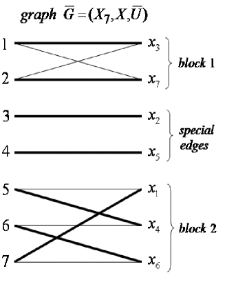
Figure 6: Example of a graph $\bar{G}=(X_{7},X,\bar{U})$ with two special edges and two blocks.

The blocks of graph $\bar{G}$ may be computed in $O(k)$ time, e. g. by means of the "depth first" algorithm [14]. The special edges and maximal matchings in blocks may be found easily in $O(k)$ time.

Therefore, the problem ${\mathcal{I}}$ is solvable by the following algorithm: Build the bipartite graph $\bar{G}$, identify the set of special edges and blocks and find all maximal matchings in blocks. Enumerate all perfect matchings $W\in\mathcal{W}$ of graph $\bar{G}$ by combining the maximal matchings of blocks and joining them with special edges. Assign the corresponding solution $f\in F$ to each $W\in\mathcal{W}$ and compute $\rho(f)$. As a result one can find $f^{*}\in F$, such that $\rho(f^{*})=\min\limits_{f\in F}\rho(f)$.

Note that $|F|=|\mathcal{W}|=2^{q(\bar{G})}$, so the time complexity of the above algorithm is $O(k2^{q(\bar{G})})$, where ${q(\bar{G})\leqslant\lfloor\frac{k}{2}\rfloor}$ and this bound is tight. Below we propose a modification of this algorithm with time complexity $O(q(\bar{G})\cdot 2^{q(\bar{G})})$.

Let us carry out some preliminary computations before enumerating all possible combinations of maximal matchings in blocks in order to speed up the evaluation of objective function. We will call a contact between block $j$ and block $j^{\prime}\neq j$ (or between block $j$ and a special edge) the pair of vertices $(i,i+1)$ in the left-hand part of graph $\bar{G}$, such that one of the vertices belongs to the block $j$ and the other one belongs to block $j^{\prime}$ (or the special edge). A contact inside a block will mean a pair of vertices in the left-hand part of a block, if their indices differ exactly by one.

For each block $j,$ ${j=1,\dots,q(\bar{G})}$, let us check the presence of contacts inside the block $j$, between the block $j$ and all special edges, and between the block $j$ and every other block. The time complexity of checking for contacts all vertices in the left-hand part of a block is $O(k)$.

Consider a block ${j}$. If a contact $(i,i+1)$ is present inside this block, then each of the two maximal matchings $w^{0,j}$ and $w^{1,j}$ in this block corresponds to an arc of graph $G$. Also, if block $j$ has a contact to a special edge, each of the two maximal matchings $w^{0,j}$ and $w^{1,j}$ also corresponds to an arc of graph $G$. For each of the matchings $w^{k,j},\ k=0,1$, let the sum of the weights of arcs corresponding to the contacts inside block $j$ and the contacts to special edges be denoted by $P^{k}_{j}$.

If block ${j}$ contacts to block ${j^{\prime},\ j^{\prime}\neq j}$, then each combination of the maximal matchings of these blocks corresponds to an arc of graph $G$ for any contact $(i,i+1)$ between the blocks. If a maximal matching is chosen in each of the blocks, one can sum up the weights of the arcs in $G$ that correspond to all contacts between blocks ${j}$ and ${j^{\prime}}$. This yields four values which we denote by $P^{(0,0)}_{jj^{\prime}}$, $P^{(0,1)}_{jj^{\prime}}$, $P^{(1,0)}_{jj^{\prime}}$ and $P^{(1,1)}_{jj^{\prime}}$, where the superscripts identify the matchings chosen in each of the blocks $j$ and $j^{\prime}$ accordingly.

The above mentioned sums are computed for each block, so the overall time complexity of this pre-processing procedure is $O(k\cdot q(\bar{G}))$.

Now all possible combinations of the maximal matchings in blocks may be enumerated using a Grey code (see e.g. [45]) so that the next combination differs from the previous one by altering a maximal matching only in one of the blocks. Let the binary vector $\delta=(\delta_{1},\dots,\delta_{q(\bar{G})})$ define assignments of the maximal matchings in blocks. Namely, $\delta_{j}=0$, if the matching $w^{0,j}$ is chosen in block $j$; otherwise (if the matching $w^{1,j}$ is chosen in block $j$), we have $\delta_{j}=1$. This way every vector $\delta$ is bijectively mapped into a feasible solution $f_{\delta}$ to problem ${\mathcal{I}}$.

In the process of enumeration, a step from the current vector $\bar{\delta}$ to the next vector $\delta$ changes the maximal matching in one of the blocks $j$. The new value of objective function $\rho(f_{\delta})$ may be computed via the current value $\rho(f_{\bar{\delta}})$ by the formula $\rho(f_{\delta})=\rho(f_{\bar{\delta}})-P^{{\bar{\delta}}_{j}}_{j}+P^{{\delta}_{j}}_{j}-\sum\limits_{j^{\prime}\in A(j)}P^{({\bar{\delta}}_{j},{\bar{\delta}}_{j^{\prime}})}_{jj^{\prime}}+\sum\limits_{j^{\prime}\in A(j)}P^{({\delta}_{j},{\delta}_{j^{\prime}})}_{jj^{\prime}}$, where $A(j)$ is the set of blocks contacting to block $j$. Obviously, $|A(j)|\leqslant q(\bar{G})$, so updating the objective function value for the next solution requires $O(q(\bar{G}))$ time, and the overall time complexity of the modified algorithm for solving Problem ${\mathcal{I}}$ is $O(q(\bar{G})\cdot 2^{q(\bar{G})})$.

Therefore, the ORP for $1|s_{vu}|C_{\max}$, as well as Problem ${\mathcal{I}}$, is solvable in $O(q(\bar{G})\cdot 2^{q(\bar{G})})$ time. Below it will be shown that for almost all pairs of parent solutions ${q(\bar{G})}\leqslant 1.1\cdot{\rm ln}(k)$, i. e. the cardinality of the set of feasible solutions in almost all instances of the ORP for $1|s_{vu}|C_{\max}$ is at most $k$ and these instances are solvable in $O(k\cdot{\rm ln}(k))$ time.

Definition 3

[46] A graph ${\bar{G}=(X_{k},X,\bar{U})}$ is called "good" if ${q(\bar{G})\leqslant 1.1\cdot{\rm ln}(k)}$; otherwise it is called "bad".

Definition 4

A pair of parent solutions $\{\pi^{1},\pi^{2}\}$ is called "good" if the graph $\bar{G}=(X_{k},X,\bar{U})$ corresponding to these parent solutions is "good"; otherwise the pair $\{\pi^{1},\pi^{2}\}$ is called "bad".

Note that instead of constant $1.1$ in Definition 3 one may choose any other constant equal to $1+\varepsilon,$ where $\varepsilon\in(0,{\rm log}_{2}(e)-1]$. Given such a constant, the ORP has at most $k$ feasible solutions and it is solvable in $O(k{\rm ln}(k))$ time.

The following notation will be used below:

• Let $\bar{\Im}_{k}$ be the set of "good" graphs and let $\tilde{\Im}_{k}$ denote the set of "bad" graphs.

• Let $\bar{\Re}_{k}$ be the set of "good" pairs of parent solutions and let $\tilde{\Re}_{k}$ be the set of "bad" pairs of parent solutions.

• Denote ${\Im}_{k}=\bar{\Im}_{k}\cup\tilde{\Im}_{k}$, ${\Re}_{k}=\bar{\Re}_{k}\cup\tilde{\Re}_{k}$.

• Let ${S}_{l}$ be the set of permutations of the set $\{1,\dots,l\}$, which do not contain the cycles of length 1.

• Let $\bar{S}_{l}$ denote the set of permutations from $S_{l}$, where the number of cycles is at most ${1.1\cdot{\rm ln}(l)}$.

• Denote $\tilde{S}_{l}={S}_{l}\backslash\bar{S}_{l}$.

The results of A.I. Serdyukov from [46] imply

Proposition 6

$|\tilde{S}_{l}|/|\bar{S}_{l}|\longrightarrow 0$ as $l\to\infty$.

The next theorem is proved by the means of Proposition 6.

Theorem 10

[25] $|\bar{\Re}_{k}|/|{\Re}_{k}|\longrightarrow 1$ as $k\to\infty$.

Proof. The proof consists of two stages: first we estimate the numbers of "good" and "bad" graphs, and after that we estimate the numbers of "good" and "bad" pairs of parent solutions.

The values $|\bar{\Im}_{k}|$ and $|\tilde{\Im}_{k}|$ may be bounded using the approach from [46]. To this end assign any permutation $\sigma\in{S}_{l}$, $l\leqslant k$, a set of bi-partite graphs ${{\Im}_{k}(\sigma)\subset{\Im}_{k}}$ as follows. First of all let us assign an arbitrary set of $k-l$ edges to be special. The non-special vertices $\{i_{1},i_{2},\dots,i_{l}\}\subset X_{k}$ of the left-hand part, where $i_{j}<i_{j+1},\ j=1,\dots,l-1$, are now partitioned into $\xi(\sigma)$ blocks, where $\xi(\sigma)$ is the number of cycles in permutation $\sigma$. Every cycle $(t_{1},t_{2},\dots,t_{r})$ in permutation $\sigma$ corresponds to some sequence of vertices with indices $\{i_{t_{1}},i_{t_{2}},\dots,i_{t_{r}}\}$ belonging to the block associated with this cycle. Finally, it is ensured that for each pair of vertices $\{i_{t_{j}},\ i_{t_{j+1}}\}$, $j=1,\dots,r-1$, as well as for the pair $\{i_{t_{r}},\ i_{t_{1}}\},$ there exists a vertex in the right-hand part $X$ adjacent to both vertices of the pair.

Consider a permutation $\sigma={1\ 2\ 3\ 4\ 5\choose 2\ 3\ 1\ 5\ 4}\in S_{5}$ with cycles $c_{1}=(1,2,3)$ and $c_{2}=(4,5)$. Two examples of graphs from class ${{\Im}_{7}(\sigma)}$ are given in Fig. 7. Here block $j$ corresponds to cycle $c_{j}$, $j=1,2$.

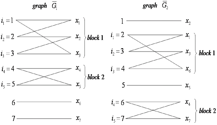
Figure 7: Examples of graphs from class ${{\Im}_{7}(\sigma)}$, where $\sigma={1\ 2\ 3\ 4\ 5\choose 2\ 3\ 1\ 5\ 4}\in S_{5}$.

There are $k!$ ways to associate vertices of the left-hand pert to vertices of the right-hand part, therefore the number of different graphs from class ${\Im}_{k}(\sigma)$, $\sigma\in{S}_{l}$, $l\leqslant k$, is $|{\Im}_{k}(\sigma)|=C_{k}^{l}\frac{k!}{2^{\xi_{1}(\sigma)}}$, where $\xi_{1}(\sigma)$ is the number of cycles of length two in permutation $\sigma$. Division by $2^{\xi_{1}(\sigma)}$ here is due to the fact that for each block that corresponds to a cycle of length two in $\sigma$, there are two equivalent ways to number the vertices in its right-hand part.

Let ${\sigma=c_{1}c_{2}\dots c_{\xi(\sigma)}}$ be a permutation from set ${S}_{l}$, represented by cycles $c_{i}$, ${i=1,\dots,\xi(\sigma)},$ and let $c_{j}$ be an arbitrary cycle of permutation $\sigma$ of length at least three, $1\leqslant j\leqslant\xi(\sigma)$. Permutation $\sigma$ may be transformed into permutation $\sigma^{1}$,

$$\sigma^{1}=c_{1}c_{2}\dots c_{j-1}c_{j}^{-1}c_{j+1}\dots c_{\xi(\sigma),}$$ (34)

by reversing the cycle $c_{j}$. Clearly, permutation $\sigma^{1}$ induces the same subset of graphs in class ${\Im}_{k}$ as the permutation $\sigma$ does. Thus any two permutations $\sigma^{1}$ and $\sigma^{2}$ from set ${S}_{l}$, $l\leqslant k$, induce the same subset of graphs in ${\Im}_{k}$, if one of these permutations may be obtained from the other one by several transformations of the form (34). Otherwise the two induced subsets of graphs do not intersect. Besides that ${\Im}_{k}(\sigma^{1})\cap{\Im}_{k}(\sigma^{2})=\emptyset$ if $\sigma^{1}\in{S}_{l_{1}}$, $\sigma^{2}\in{S}_{l_{2}}$, $l_{1}\neq l_{2}$.

On one hand, if $\sigma\in\bar{S}_{l}$, $l\leqslant k$, then ${\Im}_{k}(\sigma)\subseteq{\bar{\Im}}_{k}$. On the other hand, if $\sigma\in\tilde{S}_{l}$, $l<k$, then either ${\Im}_{k}(\sigma)\subseteq{\bar{\Im}}_{k}$ or, alternatively, ${\Im}_{k}(\sigma)\subseteq{\tilde{\Im}}_{k}$ may hold. Therefore,

$$|\bar{\Im}_{k}|\geqslant\sum_{l=2}^{k}\sum_{\sigma\in\bar{S}_{l}}C_{k}^{l}\frac{k!}{2^{\xi_{1}(\sigma)}2^{\xi(\sigma)-\xi_{1}(\sigma)}}=\sum_{l=2}^{k}\sum_{\sigma\in\bar{S}_{l}}C_{k}^{l}\frac{k!}{2^{\xi(\sigma)}},$$ (35)

$$|\tilde{\Im}_{k}|\leqslant\sum_{l=\lfloor 1.1\cdot{\rm ln}(k)\rfloor}^{k}\sum_{\sigma\in\tilde{S}_{l}}C_{k}^{l}\frac{k!}{2^{\xi_{1}(\sigma)}2^{\xi(\sigma)-\xi_{1}(\sigma)}}=\sum_{l=\lfloor 1.1\cdot{\rm ln}(k)\rfloor}^{k}\sum_{\sigma\in\tilde{S}_{l}}C_{k}^{l}\frac{k!}{2^{\xi(\sigma)}}.\\$$ (36)

Now let us estimate the cardinality of sets $\bar{\Re}_{k}$ and $\tilde{\Re}_{k}$ to complete the proof. Recall that every graph ${\bar{G}\in{\Im}_{k}(\sigma),}$ $\sigma\in{S}_{l},$ $l\leqslant k$ has $\xi(\sigma)$ blocks. The set of edges of any block $j$, ${j=1,\dots,\xi(\sigma)}$, is partitioned into the maximal matchings denoted by $w^{j}=\{(i_{1},x^{i_{1}}),(i_{2},x^{i_{2}}),\dots,(i_{m_{j}},x^{i_{m_{j}}})\}$ and $\bar{w}^{j}=\{(i_{1},\bar{x}^{i_{1}}),(i_{2},\bar{x}^{i_{2}}),\dots,(i_{m_{j}},\bar{x}^{i_{m_{j}}})\}$. Then in any instance of the ORP for problem $1|s_{vu}|C_{\max}$, that induces the graph $\bar{G}$, either $\pi^{1}_{i_{m}}=x^{i_{m}}$, $\pi^{2}_{i_{m}}=\bar{x}^{i_{m}}$, $m=1,\dots,m_{j}$, or $\pi^{1}_{i_{m}}=\bar{x}^{i_{m}}$, $\pi^{2}_{i_{m}}={x}^{i_{m}}$, $m=1,\dots,m_{j}$, for all $j=1,\dots,\xi(\sigma)$. Consequently every bipartite graph from class ${\Im}_{k}(\sigma)$ corresponds to $2^{\xi(\sigma)}$ pairs of parent solutions (where pairs $\pi^{1}=a$, $\pi^{2}=b$ and $\pi^{1}=b$, $\pi^{2}=a$ are assumed to be different), then in view of (35) and (36) we have:

$$|\bar{\Re}_{k}|\geqslant\sum_{l=2}^{k}\sum_{\sigma\in\bar{S}_{l}}C_{k}^{l}\frac{k!}{2^{\xi(\sigma)}}2^{\xi(\sigma)}\geqslant\sum_{l=\lfloor 1.1\cdot{\rm ln}(k)\rfloor}^{k}|\bar{S}_{l}|C_{k}^{l}k!,$$ (37)

$$|\tilde{\Re}_{k}|\leqslant\sum_{l=\lfloor 1.1\cdot{\rm ln}(k)\rfloor}^{k}\sum_{\sigma\in\tilde{S}_{l}}C_{k}^{l}\frac{k!}{2^{\xi(\sigma)}}2^{\xi(\sigma)}=\sum_{l=\lfloor 1.1\cdot{\rm ln}(k)\rfloor}^{k}|\tilde{S}_{l}|C_{k}^{l}k!.$$ (38)

Now assuming $\psi(k)=\max\limits_{l=\lfloor 1.1\cdot{\rm ln}(k)\rfloor,\dots,k}|\tilde{S}_{l}|/|\bar{S}_{l}|$ and taking into account (37), (38) and Proposition 6, we obtain

$$|\tilde{\Re}_{k}|/|\bar{\Re}_{k}|\leqslant\psi(k)\to 0\mbox{ as }k\to\infty.$$ (39)

Finally, the statement of the theorem follows from (39). $\Box$

Note that the algorithm proposed for solving the ORP for $1|s_{vu}|C_{\max}$ may be generalized to solve the ORPs for other problems with similar solutions encoding (examples of such problems may be found in [28, 48, 49]). The time complexity of the algorithm in these cases would depend on the time required to evaluate an objective function.

Theorems 8 and 9 imply NP-hardness of the ORPs for a family of more general scheduling problems, where the number of machines may be greater than 1 and each job may be performed in several modes, using one or more machines, see e.g. [24].

7 Conclusion

We have shown that optimal recombination may be efficiently carried out for many important NP-hard optimization problems. The well-known reductions between the NP optimization problems turned out to be useful in development of polynomial-time optimal recombination procedures. We have observed that the choice of solutions encoding has a significant influence upon the complexity of the optimal recombination problems and introduction of additional variables can sometimes simplify the task (compare Corollary 2 and Proposition 3). The question of practical utility of such simplifications remains open, since the additional redundancy in representation increases the number of constraints in the ORP. This trade-off may be studied in further research.

Another open question is related to the trade-off between the complexity of optimal recombination and its impact on the efficiency of an evolutionary algorithm (e.g. in terms of optimization time). The theoretical methods proposed in [17] and [41] may be helpful in runtime analysis of GAs with optimal recombination.

All of the polynomially solvable cases of the optimal recombination problems considered above rely upon the efficient deterministic algorithms for the Max-Flow/Min-Cut Problem (or the Maximum Matching Problem in the unweighted case). However, the crossover operator was initially introduced as a randomized operator in genetic algorithms [32]. As a compromise approach one can solve the optimal recombination problem approximately or solve it optimally but not in all occasions. Examples of the genetic algorithms using this approach may be found in [12, 19, 21, 24].

The obtained results indicate that optimal recombination for many NP-hard optimization problems is also NP-hard. It is natural to expect, however, that the ORP instances emerging in a GA would often have much smaller dimensions, compared to the original problem. The average dimensions of the ORP might decrease in process of GA execution, as the individuals gain more common genes. In such situations even the NP-hard ORP may turn out to be solvable in practice by the exact methods, see e.g. [3, 19, 24].

In this paper, we did not discuss the population management strategies of the GAs with optimal recombination. Due to fast localization of the search process such GAs, it is often important to provide a sufficiently large initial population and employ some mechanism for adaptation of the mutation strength. Interesting techniques that maintain the diversity of population by constructing the second offspring, as different from the optimal offspring as possible, can be found in [2] and [8]. It is likely that the general schemes of the evolutionary algorithms and the procedures of parameter adaptation require some revision when the optimal recombination is used (see e.g. [19, 49]).

8 Acknowledgements

Partially supported by Russian Foundation for Basic Research grants 12-01-00122 and 13-01-00862 and by Presidium SB RAS (project 7B).

References

- [1] Agarwal, C.C., Orlin, J.B. and Tai, R.P., ‘‘Optimized crossover for the independent set problem’’, working paper no. 3787-95, Massachusetts Institute of Technology, 1995.
- [2] Aggarwal, C.C., Orlin, J.B. and Tai, R.P., ‘‘An optimized crossover for maximum independent set’’, Operations Research, 45 (1997) 225-234.
- [3] Ahuja, R.K., Orlin, J.B. and Tiwari, A., ‘‘A greedy genetic algorithm for the quadratic assignment problem’’, Computers & Operations Research, 27 (2000) 917-934.
- [4] Alekseeva, E., Kochetov, Yu. and Plyasunov, A., ‘‘Complexity of local search for the -median problem’’, European Journal of Operational Research, 191 (2008) 736-752.
- [5] Ausiello, G., Crescenzi, P., Gambosi, G. et al., Complexity and approximation: Combinatorial optimization problems and their approximability properties, Berlin, Springer-Verlag, 1999.
- [6] Balas, E. and Niehaus, W., ‘‘A max-flow based procedure for finding heavy cliques in vertex-weighted graphs’’, MSRR no. 612, Carnegie-Mellon University, 1995.
- [7] Balas, E. and Niehaus, W., ‘‘Finding large cliques in arbitrary graphs by bipartite matching’’, DIMACS Series in Discrete Mathematics and Theoretical Computer Science, Ed. by D. Johnson and M. Trick, Vol. 26, Providence, RI, American Mathematical Society, 1996, 29-49.
- [8] Balas, E. and Niehaus, W., ‘‘Optimized crossover-based genetic algorithms for the maximum cardinality and maximum weight clique problems’’, Journal of Heuristics, 4 (2) (1998) 107-122.
- [9] Beresnev, V.L., Gimady, Ed.Kh. and Dementev, V. T., Extremal problems of standardization, Novosibirsk, Nauka, 1978 (in Russian).
- [10] Berge, C. The theory of graphs and its applications, New York, NY, John Wiley & Sons Inc., 1962.
- [11] Beyer, H.-G., Schwefel, H.-P. and Wegener, I., ‘‘How to analyse evolutionary algorithms’’, Theoretical Computer Science, 287 (2002) 101-130.
- [12] Borisovsky, P., Dolgui, A. and Eremeev, A., ‘‘Genetic algorithms for a supply management problem: MIP-recombination vs greedy decoder’’, European Journal of Operational Research, 195 (3) (2009) 770-779.
- [13] Cook, W. and Seymour, P., ‘‘Tour merging via branch-decomposition’’, INFORMS Journal on Computing, 15 (2) (2003) 233-248.
- [14] Cormen, T.H., Leiserson, C.E., Rivest, R.L., and Stein, C., Introduction to Algorithms, 2nd edition, MIT Press, 2001.
- [15] Cotta, C., ‘‘A study on allelic recombination’’, Proc. of 2003 Congress on Evolutionary Computation, Canberra, IEEE Press, 2003, 1406-1413.
- [16] Cotta, C. and Troya, J.M., ‘‘Embedding branch and bound within evolutionary algorithms’’ Applied Intelligence 18 (2003) 137-153.
- [17] Doerr, B., Happ, E. and Klein, C., ‘‘Crossover can provably be useful in evolutionary computation’’ Theoretical Computer Science 425 (2012) 17-33.
- [18] Dolgui, A. and Eremeev, A., ‘‘On complexity of optimal recombination for one-dimensional bin packing problem’’, Proc. of VIII Intern. Conf. ‘‘Dynamics of systems, mechanisms and machines’’, Vol. 3, Omsk, Omsk Polytechnical University, 2012, 25-27. (In Russian)
- [19] Dolgui, A., Eremeev, A. and Guschinskaya, O., ‘‘MIP-based GRASP and genetic algorithm for balancing transfer lines’’, Matheuristics. Hybridizing Metaheuristics and Mathematical Programming, Ed. by V. Maniezzo, T. Stutzle, and S. Voss, Berlin, Springer-Verlag, 2010, 189-208.
- [20] Eppstein, D. ‘‘The travelling salesman problem for cubic graphs’’, Journal of Graph Algorithms and Applications, 11 (1) (2007) 61-81.
- [21] Eremeev, A.V., ‘‘A Genetic algorithm with a non-binary representation for the set covering problem’’ Proc. of Operations Research (OR’98), Berlin, Springer-Verlag, 1999, 175-181.
- [22] Eremeev, A.V., ‘‘On complexity of optimal recombination for binary representations of solutions’’, Evolutionary Computation, 16 (1) (2008) 127-147.
- [23] Eremeev, A.V., ‘‘On complexity of optimal recombination for the travelling salesman problem’’ Proc. of Evolutionary Computation in Combinatorial Optimization (EvoCOP 2011), LNCS Vol. 6622, Berlin, Springer Verlag, 2011, 215-225.
- [24] Eremeev, A.V. and Kovalenko, J.V., ‘‘On scheduling with technology based machines grouping’’, Diskretnyi analys i issledovanie operacii, 18 (5) (2011) 54-79. (In Russian)
- [25] Eremeev, A.V. and Kovalenko, J.V., ‘‘On complexity of optimal recombination for one scheduling problem with setup times’’, Diskretnyi analys i issledovanie operacii, 19 (3) (2012) 13-26. (In Russian)
- [26] Garey, M. and Johnson, D., Computers and intractability. A guide to the theory of NP-completeness. W.H. Freeman and Company, San Francisco, CA, 1979.
- [27] Glover, F., Laguna, M. and Marti, R., ‘‘Fundamentals of scatter search and path relinking’’, Control and Cybernetics 29 (3) (2000) 653-684.
- [28] Hazir, Ö., Günalay, Y., Erel, E. ‘‘Customer order scheduling problem: A comparative metaheuristics study’’, International Journal of Advanced Manufacturing Technology, 37 (2008) 589-598.
- [29] Held, M. and Karp, R.M. ‘‘A dynamic programming approach to sequencing problems’’, SIAM Journal on Applied Mathematics, 10 (1962) 196-210.
- [30] Hochbaum, D.S. ‘‘Approximating covering and packing problems: set cover, vertex cover, independent set, and related problems’’, Approximation Algorithms for NP-Hard Problems, Ed. by D. Hochbaum, Boston, PWS Publishing Company, 1997, 94-143.
- [31] Hohn, C. and Reeves, C.R., ‘‘Graph partitioning using genetic algorithms’’, Proc. of the 2nd Int. Conf. on Massively Parallel Computing Systems, Los Alamitos, CA, IEEE Press, 1996, 31-38.
- [32] Holland, J., Adaptation in natural and artificial systems, Ann Arbor, University of Michigan Press, 1975.
- [33] Itai, A., Papadimitriou, C.H. and Szwarcfiter, J.L., ‘‘Hamilton paths in grid graphs’’ SIAM Journal on Computing, 11 (4) (1982) 676-686.
- [34] Jansen, T. and Wegener, I., ‘‘On the analysis of evolutionary algorithms – a proof that crossover really can help’’, Algorithmica, 34 (1) (2002) 47-66.
- [35] Mukhacheva, E.A. and Mukhacheva, A.S., ‘‘L.V. Kantorovich and cutting-packing problems: New approaches to combinatorial problems of linear cutting and rectangular packing’’, Journal of Mathematical Sciences, 133 (4) (2006) 1504-1512.
- [36] Karp, R.M., ‘‘Reducibility among combinatorial problems’’, Proc. of a Symp. on the Complexity of Computer Computations, Ed by R.E. Miller and J.W. Thatcher, The IBM Research Symposia Series, New York, NY, Plenum Press, 1972, pp. 85-103.
- [37] Korte, B. and Vygen, J., Combinatorial Optimization. Theory and Algorithms, 3rd edition, Berlin, Springer-Verlag, 2005.
- [38] Krarup, J. and Pruzan, P., ‘‘The simple plant location problem: survey and synthesis’’, European Journal of Operational Research, 12 (1983) 36-81.
- [39] Lourenço, H., Paixo, J. and Portugal, R., ‘‘Multiobjective metaheuristics for the bus driver scheduling problem’’ Transportation Science, 35 (2001) 331-343.
- [40] Papadimitriou, C.H. and Steiglitz, K., Combinatorial Optimization: Algorithms and Complexity, Upper Saddle River, NJ, Prentice-Hall, 1982.
- [41] Rabani, Y., Rabinovich, Y. and Sinclair A., ‘‘A computational view of population genetics’’, Random Structures and Algorithms 12 (1998) 314-334.
- [42] Radcliffe, N.J., ‘‘The algebra of genetic algorithms’’, Annals of Mathemathics and Artificial Intelligence, 10 (4) (1994) 339-384.
- [43] Reeves, C.R. ‘‘Genetic algorithms for the operations researcher’’, INFORMS Journal on Computing 9 (3) (1997) 231-250.
- [44] Reeves, C.R. and Rowe, J.E., Genetic algorithms: principles and perspectives, Norwell, MA, Kluwer Acad. Pbs., 2002.
- [45] Reingold, E.M., Nievergelt, J. and Deo, N. Combinatorial algorithms: Theory and practice, Englewood Cliffs, Prentice-Hall, 1977.
- [46] Serdyukov, A.I. ‘‘On travelling salesman problem with prohibitions’’, Upravlaemye systemi, 17 (1978) 80-86. (In Russian)
- [47] Schuurman, P. and Woeginger, G., Approximation schemes – a tutorial, Eindhoven University of Technology, 2006.
- [48] Tanaev, V.S., Kovalyov, M.Y. and Shafransky, Y.M. Scheduling Theory. Group Technologies, Minsk, Institute of Technical Cybernetics NAN of Belarus, 1998. (In Russian)
- [49] Yagiura, M., Ibaraki, T., ‘‘The use of dynamic programming in genetic algorithms for permutation problems’’, European Journal of Operational Research, 92 (1996) 387-401.
- [50] Yankovskaya, A.E., ‘‘Test pattern recognition with the use of genetic algorithms’’, Pattern Recognition and Image Analysis, 9 (1) (1999) 121-123.