Residual discrete symmetry of the five-state clock model

Abstract

It is well-known that the $q$-state clock model can exhibit a Kosterlitz-Thouless (KT) transition if $q$ is equal to or greater than a certain threshold, which has been believed to be five. However, recent numerical studies indicate that helicity modulus does not vanish in the high-temperature phase of the five-state clock model as predicted by the KT scenario. By performing Monte Carlo calculations under the fluctuating twist boundary condition, we show that it is because the five-state clock model does not have the fully continuous $U(1)$ symmetry even in the high-temperature phase while the six-state clock model does. We suggest that the upper transition of the five-state clock model is actually a weaker cousin of the KT transition so that it is $q\geq 6$ that exhibits the genuine KT behavior.

I Introduction

Theories of critical phenomena in low dimensions are now quite well established due to the concepts of the renormalization group (RG) and universality. The two-dimensional (2D) Ising model and the 2D $XY$ model are two classical model systems that have considerably enhanced our understanding of these concepts. While the former exhibits an order-disorder phase transition, the physics of the latter model is better described in terms of vortex-antivortex unbinding, where the Kosterlitz-Thouless (KT) picture emerges Kosterlitz and Thouless (1973); *kost. Closely related to these models, one may also consider the 2D $q$-state clock model defined by the following Hamiltonian:

$$H=-J\sum_{\left<ij\right>}\cos(\theta_{i}-\theta_{j}),$$ (1)

where $J$ means interaction strength, the summation is over the nearest neighbors, and $\theta_{i}=2\pi n_{i}/q$ with $n_{i}=0,\ldots,q-1$. As can be easily seen, this model has been extensively studied as a bridge between the Ising model ($q=2$) and the $XY$ model ($q\rightarrow\infty$). But it does not mean that $q\rightarrow\infty$ is actually required for a KT transition to be observed: Rather, the KT behavior becomes possible for $q>q_{c}$ with an intermediate quasi-ordered massless phase between an ordered phase at low temperature and a disordered phase at high temperature. A hand-waving RG argument is that domain walls get so floppy to effectively provide block spins with the continuous $U(1)$ symmetry over large length scales Einhorn et al. (1980). In order to estimate $q_{c}$, let us generalize Eq. (1) so that

$$H=\sum_{\left<ij\right>}V(\theta_{i}-\theta_{j}),$$

where the spin-interaction potential $V$ has the $Z_{q}$ symmetry. The Villain $q$-state clock model chooses, for example,

$$V(\phi)=-\frac{J}{\beta}\ln\left\{\sum_{n=-\infty}^{\infty}\exp\left[-\beta(\phi-2\pi n)^{2}/2\right]\right\},$$

where $\beta\equiv 1/(k_{B}T)$ with the Boltzmann constant $k_{B}$ and temperature $T$. This potential form has been introduced to separate the vortex degrees of freedom from the spin-wave degrees of freedom as an approximate version of the $XY$ model Savit (1980). This Villain clock model on the square lattice possesses self-duality Savit (1980), predicting that $q_{c}=4$ based on the following argument Elitzur et al. (1979): Suppose that there are only two phases. Then, the phase transition should occur at the dual point $T^{\rm Villain}_{d}=2\pi/q$. The Villain $XY$ model has a transition temperature around $T^{\rm Villain}_{\rm KT}\sim 1.35$. For $q>4$, therefore, $T^{\rm Villain}_{d}$ becomes lower than $T^{\rm Villain}_{\rm KT}$. However, this is against the correlation inequality Savit (1980), which says that

$$\left<\cos(\theta_{i}-\theta_{j})\right>^{\rm Villain}_{q}\geq\left<\cos(\theta_{i}-\theta_{j})\right>^{\rm Villain}_{XY},$$

where $i$ and $j$ are arbitrary spin indices and the brakets mean statistical averages of the Villain $q$-state clock model and that of the Villain $XY$ model, respectively, at the same temperature. It expresses an intuitively obvious idea that ordering is generally weaker in the latter model since it has a greater number of possible spin configurations, and this sort of statement holds even if we work with the cosine potential. In short, the transition temperature of the Villain $q$-state clock model cannot be lower than $T^{\rm Villain}_{\rm KT}$, contradicting the duality argument in the two-phase picture. Therefore, the two-phase picture is not valid and we are forced to have three phases at least for $q>4$. The same conclusion can be drawn for the triangular and honeycomb lattices as well Cardy (1980).

Since this argument relies on the specific choice of $V(\phi)$ in the Villain form, one might wonder if the same conclusion can be drawn for the usual clock model with the cosine potential. For instance, a recent claim was $q_{c}=7$ based on helicity modulus Lapilli et al. (2006), though more recent calculations have confirmed a normal KT transition for $q=6$ Baek et al. (2010). Since the four-state clock model exactly belongs to the Ising universality class Suzuki (1967), the only remaining case to consider is $q=5$. Although the Migdal-Kadanoff RG transformation predicts only two phases Nishimori (1979), there is ample evidence that this five-state clock model does have three phases Tobochnik (1982); Bonnier and Leroyer (1991); Borisenko et al. (2011), and theoretical arguments for the three-phase picture have been motivated and supported by these observations. We first calculate the conformal charge $c$ from the leading finite-size correction of the free energy on semi-infinite strips of the square geometry Cardy (1986), and this also indicates the existence of a temperature region with $c=1$ as in the six-state clock model [compare Fig. 1(a) and 1(b)]. Even if not completely rigorous, a convincing argument for the three-phase picture originates from a field-theoretic construction Fateev and Zamolodchikov (1982), which shows that there exists a conformally invariant point with conformal charge $c=8/7$ between the Potts model and the clock model, and conjectures that this is where the two critical lines merge *[Thisspecialpointcorrespondsto$p=2.01677$and$β=5.27413$intermsofthegeneralizedclockmodelparameterizedby$p$asfoundin][.]q8. This conjecture is found consistent with numerical results Alcaraz (1987); Bonnier and Rouidi (1990); Bonnier (1991). In short, the dominant consensus is that the five-state clock model belongs to the same universality class as the Villain five-state clock model, where one KT transition and its dual separate three phases.

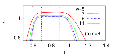
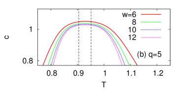
Figure 1: (Color online) (a) Conformal charge of the six-state clock model estimated by using semi-infinite strips with different widths $w$. The vertical lines represent $T_{c1}$ and $T_{c2}$ obtained in Ref. Tomita and Okabe (2002). (b) The same quantity for the five-state clock model, where the vertical lines represent $T_{c1}$ and $T_{c2}$ obtained in Ref. Borisenko et al. (2011). The free energy of each finite-sized system is calculated by using the transfer-matrix method Blöte and Nightingale (1982); *blote2; *foster and the bulk free energy is obtained by the Bulirsch-Stoer extrapolation algorithm Henkel and Schütz (1988). Note the convergence to $c=1$ as $w$ grows in both the cases.

Figure 2: Phase diagram of the $q$-state clock model. The transition points for $q>4$ are taken from Refs. Borisenko et al. (2011); Tomita and Okabe (2002); Hasenbusch and Pinn (1997), and the solid lines are guides to eyes. Note that both the transition points for $q=5$ are above the dotted horizontal line, representing $T_{\rm KT}$.

However, we have observed that helicity modulus of the five-state clock model does not vanish at the upper transition Baek and Minnhagen (2010), which casts doubt on its KT nature. That is, if the system underwent a KT transition, this quantity would show a jump to zero Nelson and Kosterlitz (1977); *minnhagen. Here, the helicity modulus is defined as response to an infinitesimal twist $\Delta$ across the system in the $x$ direction:

$$\Upsilon\equiv\left.\frac{\partial^{2}F}{\partial\Delta^{2}}\right|_{\Delta=0}=\left<e\right>-L^{2}\beta\left<s^{2}\right>,$$ (2)

where $e\equiv L^{-2}\sum_{\left<ij\right>_{x}}V^{\prime\prime}(\theta_{i}-\theta_{j})$ and $s\equiv L^{-2}\sum_{\left<ij\right>_{x}}V^{\prime}(\theta_{i}-\theta_{j})$ are summed over all the links in the $x$ direction. Although extensive Monte Carlo calculations have shown that all the other features of the transition are not inconsistent with the KT picture Borisenko et al. (2011, 2012), these calculations raise further questions since the transition temperatures are estimated as $T_{c1}=0.9051(9)$ and $T_{c2}=0.9515(9)$, respectively: Estimates of the transition temperature $T_{\rm KT}$ of the $XY$ model vary among authors Olsson (1995); Tomita and Okabe (2002); Hasenbusch and Pinn (1997); *hasen2, but one can safely say $T_{\rm KT}<0.894$. The point is that $T_{\rm KT}$ is still well below the lower transition temperature of the five-state clock model, as well as the dual point $T_{d}\approx 0.9291$ Nishimori (1979); Wu (1979) (see Fig. 2). This implies a sort of prematurity in the emergence of three phases in the five-state clock model in that the duality cannot enforce it as in the Villain clock model. In addition, when the mass gap in the Hamiltonian formulation has a singularity of the following form:

$$m(\tau)\sim\exp(C\tau^{-\sigma}),$$

where $\tau$ is the reduced temperature and $C$ is a constant, the KT prediction of $\sigma=1/2$ Kosterlitz and Thouless (1973); *kost appears consistent only when $q\geq 6$, whereas it converges to $\sigma\approx 0.2$ at $q=5$ Elitzur et al. (1979); Bonnier and Rouidi (1990). Note that a second-order phase transition would be represented by $\sigma=0$. All these signatures suggest something inherently different in the five-state clock model from the six-state clock model as well as from the four-state clock model. To sum up, the situation is that the three-phase picture looks convincing in the five-state clock model, but that consistency with the KT picture is still doubtful.

In this work, we explicitly show that the nonvanishing helicity modulus of the five-state clock model means a residual five-fold symmetry, which is not completely washed away by spin fluctuations even at $T\geq T_{c2}$. It implies a possibility that the continuous $U(1)$ symmetry as in the $XY$ model sets in only when $T\rightarrow\infty$, which means a difference from the Villain formulation. After presenting our numerical results in Sec. II, we discuss a theoretical attempt to explain this feature by introducing the second length scale of vortex composites in Sec. III, and then conclude this work.

II Fluctuating twist boundary condition

In the fluctuating twist boundary condition (FTBC) Kim et al. (1999); *ftbc2, there exists interaction among the boundary spins as in the periodic boundary condition. A difference is that here we apply a gauge field that adds twist $\Delta$ in the interaction potential. If $\Delta$ is fixed at zero, it is identical to the periodic boundary condition, whereas if it is fixed at $\pi$, it corresponds to the anti-periodic boundary condition. As the name indicates, the FTBC lets the twist $\Delta$ also fluctuate in time following the Metropolis update rule. The free energy is written as $F=F(T,\Delta)$, and the probability to observe $\Delta$ at a given $K$ will be $P(T,\Delta)\propto\exp[-\beta F(T,\Delta)]$ Bennett (1976). In this way, we measure how the free energy changes as $\Delta$ varies. When $\Delta$ is a continuous variable, since $F(K,\Delta)=F(K,0)+\frac{\Delta^{2}}{2}\left.\frac{\partial^{2}F}{\partial\Delta^{2}}\right|_{\Delta=0}+\ldots$, this method provides an estimate of the helicity modulus defined in Eq. (2).

Let us begin with the 2D Ising model ($q=2$) on the square lattice. Since $\left<s^{2}\right>$ is identically zero, its helicity modulus $\Upsilon=\left<e\right>$ is proportional to the internal energy density, which obviously does not vanish at any temperature [see Eq. (2)]. On the other hand, the free-energy difference between the periodic boundary condition and the anti-periodic boundary condition becomes exponentially small as the system size grows if the temperature is higher than $T^{\rm Ising}_{c}=2/\ln(1+\sqrt{2})\approx 2.269$ in units of $J/k_{B}$. These two facts immediately suggest that the free energy $F(\Delta)$ has a smooth barrier between $\Delta=0$ and $\pi$ and another between $\Delta=0$ and $-\pi$ by symmetry. This speculation is directly confirmed in Fig. 3(a) obtained by using the FTBC, where we see that the system is disordered but preserves its up-down symmetry. It is also intuitively clear that the system begins to prefer $\Delta=0$ to $\Delta=\pm\pi$ as $T$ passes $T^{\rm Ising}_{c}$ from above so that $F(\Delta)$ changes its shape as shown in Fig. 3(a). To understand the nonvanishing $\Upsilon$ on physical grounds, it is instructive to recall that the free energy is written as $F=U-TS$ with internal energy $U=U(T,\Delta)$ and entropy $S=S(T,\Delta)$. Since the first term in Eq. (2) is related to the second derivative of $U$, the second term describing fluctuations should be related to the entropic contribution to the free-energy change. We can say that if $\Delta$ is very small, it is difficult for the system to excite domain walls whose entropy could compensate for the energy change. In this sense, the nonvanishing $\Upsilon$ means that enough domain walls, a discrete version of spin waves, are not generated to cancel out the external perturbation $\Delta$, possibly due to the finite energy scale needed to excite them.

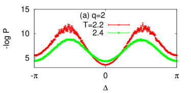
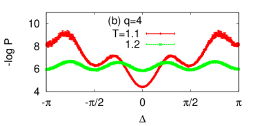
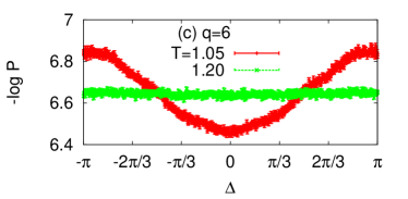
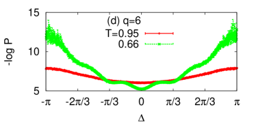
Figure 3: (Color online) Free energy $F(T,\Delta)\propto-\ln P(T,\Delta)$ where $P(T,\Delta)$ is probability of observing twist $\Delta$ under the fluctuating twist boundary condition at temperature $T$. In practice, the twist $\Delta$ is given as a $(128\times q)$-state clock spin to simulate a continuous variable. (a) The discrete symmetry is clearly detected in the disordered phase of the Ising model, and (b) the same statement can be made for the four-state clock model. (c) On the other hand, the discrete symmetry changes to the continuous $U(1)$ symmetry in the six-state clock model and (d) manifests itself only at much lower $T$. The system size is taken as $L=32$ in every case.

The four-state clock model with interaction strength $J$ has the same partition function as two independent Ising systems with interaction strength $J/2$ Suzuki (1967). This model has $c=1$ since each Ising model carries conformal charge $c=1/2$ Boyanovsky (1989), but the massless phase exists only at a single point so the model has only two phases separated at $T^{q=4}_{c}=T^{\rm Ising}_{c}/2\approx 1.135$. It is also obvious from this equivalence that $\Upsilon$ does not vanish at $T>T_{c}$, and we see how the system preserves its four-fold symmetry in Fig. 3(b). In terms of vortices, this is related to the fact that a vortex is not a really independent object but merely results from two independent Ising domain walls that happen to cross at a point.

In the six-state clock model, on the other hand, we expect from the vanishing $\Upsilon$ that the six-fold symmetry will be manifested only at $T<T_{c1}$ and is not visible at higher temperatures. In the language of the RG, it means that the system can respond to perturbations as if it were a continuous spin system on average over large length scales. Our numerical calculations on the $L\times L$ square lattice clearly support this picture as depicted in Figs. 3(c) and 3(d). Note that these results are obtained with quite a small size, i.e., $L=32$, so that the transition temperature $T_{c2}$ tends to be overestimated [see, e.g., Figs. 4(c) or 4(d)]. Nevertheless, these give us a qualitatively correct picture that remains true for larger system sizes (see Ref. Baek and Minnhagen (2010), which shows data up to $L=512$). In short, the six-state clock model effectively exhibits the continuous $U(1)$ symmetry whereby the genuine KT behavior becomes possible.

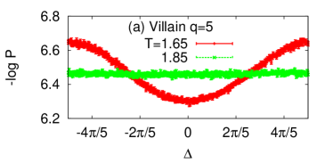
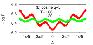
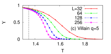
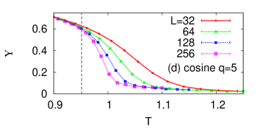
Figure 4: (Color online) (a) Free energy $F(\Delta)$ of the Villain five-state clock model [cf. Fig. 3(c)]. (b) Five-fold symmetry is clearly visible in the five-state clock model with the cosine potential. We take $L=32$ as the system size in both the cases. (c) As the system size grows in the Villain five-state clock model, the change in curvature at $\Delta=0$ [i.e., Eq. (2)] becomes sharper, approaching the universal jump to zero. The vertical line shows the critical temperature $T_{c2}^{\rm Villain}\approx 1.35$ estimated by extrapolating the size dependence of the universal jump condition $\Upsilon(T_{c}^{\rm Villain})=2T_{c}^{\rm Villain}/\pi$ Nelson and Kosterlitz (1977); *minnhagen according to the KT scenario $\tau\sim(\ln L)^{-2}$. (d) When $L$ increases in the five-state clock model, the curvature at $\Delta=0$ remains finite even above $T_{c2}\approx 0.9515$ Borisenko et al. (2011), which is represented as the vertical line.

It is interesting to see that the Villain five-state clock model also shows the same kind of behavior, supporting theoretical works based on the Villain formulation [Fig. 4(a)]. However, when the method is applied to the conventional five-state clock model to obtain $F(\Delta)$, we see that the behavior is more similar to what we observed for $q=2$ or $q=4$ than to $q=6$, in that the model exhibits its five-fold symmetry even in the disordered phase [Fig. 4(b)]. Note that the free energy $F(\Delta)$ has a curvature near $\Delta=0$, which corresponds to the nonvanishing $\Upsilon$. Therefore, the nonvanishing $\Upsilon$ signals the residual discrete symmetry above the upper transition, which remains there even if the system size grows [compare Fig. 4(c) and 4(d)], so we can conclude that the upper phase transition of the five-state clock model is not of the conventional KT type.

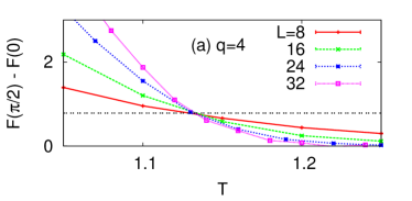
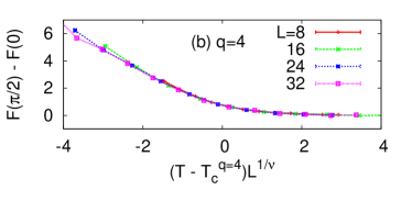
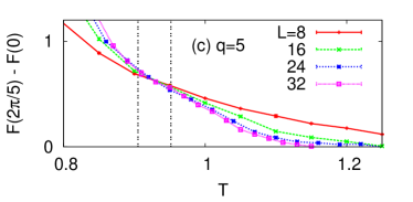
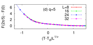
Figure 5: (Color online) (a) Interfacial free energy of the four-state clock model as a function of $T$ and (b) its scaling collapse where the exact values $T_{c}^{q=4}=1/\ln(1+\sqrt{2})\approx 1.135$ and $\nu=1$ are used. The horizontal line represents $\delta F=\pi/4$. (c) Interfacial free energy of the five-state clock model, where the two vertical lines represent $T_{c1}$ and $T_{c2}$ measured in Ref. Borisenko et al. (2011), respectively. (d) Scaling collapse attempted with the dual point $T_{d}\approx 0.9291$ Nishimori (1979) and a trial exponent $\nu=2$ used in Ref. Borisenko et al. (2011). Error bars are usually smaller than the symbol sizes.

As a brief sideline, we may consider what one would find if $\Delta$ also had the discrete $q$-fold symmetry. For the Ising model, this free-energy difference between the periodic boundary condition ($\Delta=0$) and the anti-periodic boundary condition ($\Delta=\pi$) is called the interfacial free energy. This quantity is known to have the following scaling form Nightingale et al. (1995):

$$\delta F=f\left(\tau L^{1/\nu}\right),$$ (3)

where $f$ is a scaling function with a universal amplitude $f(0)=\pi/4$ and $\nu$ is the scaling exponent for the divergence of the correlation length $\xi\sim\tau^{-\nu}$. It is straightforward to generalize the notion of the interfacial free energy to the case of the $q$-state clock model by measuring the free-energy difference caused by setting $\Delta=2\pi/q$. In other words, we define $\delta F\equiv F(2\pi/q)-F(0)$, and this quantity shows how the lower envelope of $F(\Delta)$ changes its shape. Note that the envelope is not distinguished from $F(\Delta)$ if $q\geq 6$ so that we do not have to consider such cases separately. For the four-state clock model, we observe that this method indeed yields correct scaling results [Figs. 5(a) and 5(b)]. When applied to the five-state clock model, $\delta F$ does vanish in the high-temperature phase by construction in contrast to the helicity modulus [Fig. 5(c)]. The question is then how this quantity describes the critical properties. In Ref. Borisenko et al. (2011), the authors attempt scaling collapse with $\nu=2$ under the assumption that the model undergoes a usual continuous phase transition. Using this trial exponent, we also observe reasonable scaling collapse around the dual temperature $T_{d}\approx 0.9291$ Nishimori (1979) as depicted in Fig. 5(d), but the possibility of a crossover phenomenon cannot be ruled out for such small sizes.

III Discussion and Summary

A possible reason for the peculiarity of the five-state clock model has already been argued in Refs. den Nijs (1985a, b). This theory points out a possibility that the model may have two different length scales, one from individual vortices and the other from composites of vortices. According to this scenario, the nonvanishing helicity modulus is a finite-size effect governed by the larger length scale of the composites, which will eventually become negligible in the thermodynamic limit. The correlation due to the composites is destroyed at a higher temperature called the disorder line, roughly estimated as $T_{\rm disorder}\approx[1-\cos(4\pi/5)]\approx 1.81$, where the correlated liquid becomes a Potts gas. It turns out hard to examine the existence of the second length scale with numerical calculations: If there really was a second length scale, it would have to get shorter with increasing $T$ so that the helicity modulus would then be more sensitive to the lattice size. For this reason, we have tried to observe the helicity modulus as a function of $L$ with fixing the temperature at $T=1.1$ well above $T_{c2}\approx 0.9515$. However, it appears to converge to a nonzero value at least up to $L=1024$ (see also Ref. Borisenko et al. (2012)), implying that the second length scale, if it exists, might be still greater than this size at such high $T$. We additionally note that Ref. den Nijs (1985b) suggests a conspiracy between the clock number $q=5$ and the four-fold symmetry of the square lattice: For a unit-charge vortex located at a square plaquette, the sum of angle differences around it is $2\pi$, and there are only four angle differences, each of which can take an integer multiple of $2\pi/5$. It means that there should be at least one angle difference greater than $2\pi/5$, likely to be $4\pi/5$. So the argument for the origin of the composite on the square lattice is that such a high-energy domain wall tends to appear as a double strand of two single domain walls in the vicinity of the vortex-antivortex unbinding transition, forming a correlated local structure (see Ref. Domany et al. (1980); *baltar; *knops for related discussions). However, it is not easy to extend such an argument to other 2D lattices as already noted in Ref. den Nijs (1985a), and it turns out that we need a more universal explanation because the nonvanishing helicity modulus is observed on the triangular and the honeycomb lattices as well (Fig. 6). Therefore, our observation is only partially consistent with the theory in Refs. den Nijs (1985a, b) at the moment, and it seems quite nontrivial to explain how the discrete five-fold symmetry emerges in vortex composites over more than $10^{3}$ lattice spacings. If we once again borrow the hand-waving RG argument in Sec. I Einhorn et al. (1980), our observation rather implies another possibility that the discreteness in the spin degree of freedom is not completely renormalized away with the cosine potential and that this may survive further RG transformations.

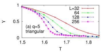
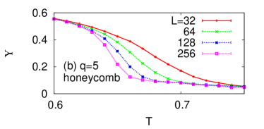
Figure 6: (Color online) Helicity modulus [Eq. (2)] of the five-state clock model (a) on the triangular lattice and (b) on the honeycomb lattice. Error bars are not larger than the symbol sizes. See also Ref. Shih and Stroud (1985) about computing $\Upsilon$ on these lattices.

In summary, we have found the origin of the nonvanishing helicity modulus numerically observed in the five-state clock model: It originates from the five-fold symmetry, which is not replaced by the continuous $U(1)$ symmetry even deep inside the high-temperature phase and clearly manifests itself under the FTBC. As a consequence, although our transfer-matrix calculation supports the three-phase picture for the five-state clock model, the nature of the transition is not fully developed to the genuine KT type, differently from its Villain-approximated version, in our Monte Carlo calculations. Since there is not enough numerical evidence for a vanishing helicity modulus in the five-state clock model, it is only for $q\geq 6$ that one can be sure of the three phases separated by a genuine KT transition and its dual, and we suggest that the transition of the five-state clock model is a weaker cousin of the KT transition.