Correlated two-neutron emission in the decay of unbound nucleus ²⁶O

Abstract

The particle unbound ²⁶O nucleus is located outside the neutron drip line, and spontaneously decays by emitting two neutrons with a relatively long life time due to the centrifugal barrier. We study the decay of this nucleus with a three-body model assuming an inert ²⁴O core and two valence neutrons. We first point out the importance of the neutron-neutron final state interaction in the observed decay energy spectrum. We also show that the energy and and angular distributions for the two emitted neutrons manifest a clear evidence for the strong neutron-neutron correlation in the three-body resonance state. In particular, we find an enhancement of two-neutron emission in back-to-back directions. This is interpreted as a consequence of dineutron correlation, with which the two neutrons are spatially localized before the emission.

Correlations among particles lead to a variety of rich phenomena in many-fermion systems, such as superconductivity and superfluidity. The spatial distribution of particles is also affected by the correlations. For many-electron systems, the Coulomb repulsion between electrons yields the so called Coulomb hole, in which the distribution of the second electron is largely suppressed in the vicinity of the first electron CN61 ; RRB78 . In atomic nuclei, in contrast, an attractive nuclear force leads to the dineutron and diproton correlations, with which two nucleons are spatially localized in the surface region of nucleiBBR67 ; CIMV84 . These nuclear correlations have attracted lots of attention recently BE91 ; Zhukov93 ; HS05 ; MMS05 ; PSS07 , in connection to physics of weakly bound nuclei.

In order to probe the inter-particle correlation, it has been a standard way in atomic physics to measure a double ionization with strong laser fieldsWSD94 ; WGW00 ; BKJ12 ; BLHE12 . It has been observed that the ionization rate is significantly enhanced due to the electronic correlation, and moreover, there is a strong momentum correlation between the two emitted electrons. The corresponding experiment in nuclear physics is the Coulomb breakup of the Borromean nuclei ¹¹Li and ⁶He, in which those nuclei are broken up to the core nuclei, ⁹Li and ⁴He, and two neutrons in the Coulomb field of a target nucleus N06 ; A99 ; NK12 . The observed breakup probabilities, especially those for the ¹¹Li nucleus, show a sharp peak in the low-energy region, which can be accounted for only by taking into account the neutron-neutron correlations. Furthermore, from the observed strength distribution, the opening angle between the valence neutrons in the ground state of the Borromean nuclei has been inferred employing the cluster sum rule N06 ; HS07 ; BH07 . For both ¹¹Li and ⁶He, the extracted opening angles were significantly smaller than the value for the independent neutrons, that is, 90 degrees, and clearly indicate the existence of the dineutron correlation.

A small drawback with the cluster sum rule approach is that it yields only an expectation value of the opening angle and a detailed angular distribution cannot be studied with this method. For this reason, the energy and the angular distributions of the emitted neutrons from the Coulomb breakup have been investigatedEB92 . However, it has been concluded that those distributions are largely determined by the properties of the neutron-core system, and thus it is difficult to acquire detailed information on the neutron-neutron correlations from the Coulomb breakup measurement HSNS09 ; KKM10 .

It is therefore desirable to seek for other probes for the nucleonic correlation. Among them, the two-proton radioactivity, that is, the spontaneous emission of two protons of proton-unbound nuclei, has been considered to be a good candidate for that purpose PKGR12 . An attractive feature of this phenomenon is that the two valence protons are emitted without an influence of disturbance of nuclei due to an external field. Very recently, the ground state two-neutron emission was discovered for ¹⁶BeSKB12 . Earlier measurements on the two-neutron emission include those for ¹⁰He J10 and ¹³Li J10 ; A08 . These are a counter part of the two-proton emission of proton-rich nuclei, corresponding to a penetration of two neutrons over a centrifugal barrier. Subsequently, the two-neutron emission was discovered also for ²⁶OLDK12 ; CSA12 and ¹³Li KLD13 . So far, the experimental data have been analyzed only with a schematic dineutron model SKB12 ; KLD13 (see also Ref. MOA12 ). Although such schematic model appears to reproduce the data, realistic three-body model calculations with configuration mixings and full neutron-neutron correlations have been clearly urged.

In this paper, we apply the three-body model with a density-dependent contact interaction between the valence neutrons to the decay problem of ²⁶O, assuming ²⁴O to be an inert core. This model has been successfully applied to describe the ground state properties and the Coulomb break-up of neutron-rich nucleiBE91 ; HS05 ; HSNS09 ; EBH97 . In order to describe the decay of neutron-unbound nucleus, we shall take into account the couplings to continuum by the Green’s function technique, which was invented in Ref. EB92 in order to describe the continuum dipole excitations of ¹¹Li. We shall discuss the role of neutron-neutron correlation in the decay probability, as well as in the energy and the angular distributions of the emitted neutrons.

In the experiment of Ref. LDK12 , the ²⁶O nucleus was produced in the single proton-knockout reaction from a secondary ²⁷F beam. We therefore first construct the ground state of ²⁷F with a three-body model, assuming the ²⁵F+$n$+$n$ structure. We then assume a sudden proton removal, that is, the ²⁵F core changes to ²⁴O keeping the configuration for the $n$+$n$ subsystem of ²⁶O to be the same as in the ground state of ²⁷F. This initial state, $\Psi_{i}$, is then evolved with the Hamiltonian for the three-body ²⁴O+$n$+$n$ system for the two-neutron decay.

We therefore consider two three-body Hamiltonians, one for the initial state ²⁵F+$n$+$n$ and the other for the final state ²⁴O+$n$+$n$. For both the systems, we use similar Hamiltonians as that in Refs. HS05 ; EBH97 ,

$$H=\hat{h}_{nC}(1)+\hat{h}_{nC}(2)+v(1,2)+\frac{\mbox{\boldmath$p$}_{1}\cdot\mbox{\boldmath$p$}_{2}}{A_{c}m},$$ (1)

where $A_{c}$ is the mass number of the core nucleus, $m$ is the nucleon mass, and $\hat{h}_{nC}$ is the single-particle (s.p.) Hamiltonian for a valence neutron interacting with the core. The last term in Eq. (1) is the two-body part of the recoil kinetic energy of the core nucleus EBH97 , while the one-body part is included in $\hat{h}_{nC}$. We use a contact interaction between the valence neutrons, $v$, given asBE91 ; HS05 ; EBH97 ,

$$v(\mbox{\boldmath$r$}_{1},\mbox{\boldmath$r$}_{2})=\delta(\mbox{\boldmath$r$}_{1}-\mbox{\boldmath$r$}_{2})\left(v_{0}+\frac{v_{\rho}}{1+\exp[(r_{1}-R_{\rho})/a_{\rho}]}\right).$$ (2)

Here, the strength $v_{0}$ is determined to be $-$857.2 MeV$\cdot$fm³ from the scattering length for the $nn$ scattering together with the cutoff energy, which we take $E_{\rm cut}=30$ MeV. See Refs.HS05 ; EBH97 for the details. The second term in Eq. (2) simulates the density dependence of the interaction. Taking $R_{\rho}=1.34\times A_{c}^{1/3}$ fm and $a_{\rho}$=0.72 fm, we adjust the value of $v_{\rho}$ to be 952.3 MeV$\cdot$fm³ so as to reproduce the experimental two-neutron separation energy of ²⁷F, $S_{\rm 2n}$=2.80(18) MeVJSM07 .

We employ a Woods-Saxon form for the s.p. potential in $\hat{h}_{nC}$. For the ²⁴O+$n+n$ system, we take $a=0.72$ fm and $R_{0}=1.25A_{c}^{1/3}$ fm with $A_{c}=24$, and determine the values of $V_{0}=-44.1$ MeV and $V_{ls}$=45.87 MeV$\cdot$fm² in order to reproduce the single-particle energies of $\epsilon_{2s_{1/2}}=-4.09(13)$ MeV and $\epsilon_{1d_{3/2}}=770^{+20}_{-10}$ keV H08 . This potential yields the width for the 1$d_{3/2}$ state of $\Gamma_{1d_{3/2}}=92.9$ keV, which is compared with the empirical value, $\Gamma_{1d_{3/2}}=172(30)$ keV H08 . For the ²⁵F+$n+n$ system, one has to modify the Woods-Saxon potential in order to take into account the presence of the valence proton in the core nucleus. The important effect comes from the tensor force between the valence proton and neutrons O05 , which primarily modifies the spin-orbit potential in the mean-field approximationSBF77 ; CSFB07 ; LBB07 . We thus use the same Woods-Saxon potential for ²⁵F+$n+n$ system as that for the ²⁴O+$n+n$ system except for the spin-orbit potential, whose strength is weakened to $V_{ls}$=33.50 MeV$\cdot$fm² in order to reproduce the energy of $1d_{3/2}$ state in ²⁷F, $\epsilon_{1d_{3/2}}=-0.811$ MeV.

With the initial wave function thus obtained, the decay energy spectrum can be computed as EB92 ,

$$\frac{dP}{dE} = \frac{1}{\pi}\Im\langle\Psi_{i}|G_{0}(E)|\Psi_{i}\rangle$$ (3)

$$-\frac{1}{\pi}\Im\langle\Psi_{i}|G_{0}(E)v(1+G_{0}(E)v)^{-1}G_{0}(E)|\Psi_{i}\rangle.$$

where $\Im$ denotes the imaginary part. In Eq. (3), $G_{0}(E)$ is the unperturbed Green’s function given by,

$$G_{0}(E)=\sum_{\rm 1,2}\frac{|(j_{1}j_{2})^{(0^{+})}\rangle\langle(j_{1}j_{2})^{(0^{+})}|}{e_{1}+e_{2}-E-i\eta},$$ (4)

where $\eta$ is an infinitesimal number and the sum includes all independent two-particle states coupled to the total angular momentum of $J=0$ with the positive parity, described by the three-body Hamiltonian for ²⁴O+$n+n$. As in our previous study for the continuum E1 excitations of the ¹¹Li nucleus HSNS09 , we have neglected the two-body part of the recoil kinetic energy in order to derive Eq. (3), while we keep all the recoil terms in constructing the initial state wave function.

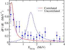
Figure 1: (Color online) The decay energy spectrum for the two-neutron emission decay of ²⁶O. The solid line denotes the result with the full inclusion of the final state neutron-neutron ($nn$) interaction, while the dashed line shows the result without the final state $nn$ interaction. The theoretical curves are drawn with a finite width of 0.21 MeV, which is the same as the experimental energy resolution. The experimental data, normalized to the unit area, are taken from Ref. LDK12 .

Figure 1 shows the decay energy spectrum obtained with Eq. (3). The solid line shows the correlated spectrum, in which the final state $nn$ interaction is fully taken into account, while the dashed line shows the result without the final state $nn$ interaction. The latter corresponds to the first term in Eq. (3). Since the width of the three-body resonance state is extremely small, which is experimentally the order of 10^-10 MeV K13 , we have introduced a finite width for a presentation purpose. That is, in evaluating the unperturbed Green’s function, Eq. (4), we set $\eta$ =0.21 MeV, that is to be the same as the experimental energy resolution. Without the final state $nn$ interaction, the two valence neutrons in ²⁶O occupy the s.p. resonance state of 1$d_{3/2}$ at 770 keV, and the peak in the decay energy spectrum appears at twice this energy. When the final state $nn$ interaction is taken into account, the peak is largely shifted towards a lower energy and appears at 0.14 MeV, in a good agreement with the experimental data.

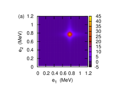
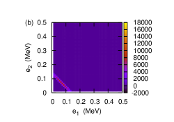
Figure 2: (Color online) The decay probability distribution for the two-neutron emission decay of ²⁶O as a function of the energies of the two emitted neutrons. Fig. 2(b) shows the correlated probability while Fig. 2(a) shows the uncorrelated probability without the final state $nn$ interactions.

The energy distribution of the two emitted neutrons is shown in Fig. 2, in which a decay amplitude is calculated to a specific two-particle final state EB92 ,

$$M_{j,l,k_{1},k_{2}} = \langle(jj)^{(00)}|1-vG_{0}+vG_{0}vG_{0}-\cdots|\Psi_{i}\rangle,$$ (5)

$$= \langle(jj)^{(00)}|(1+vG_{0})^{-1}|\Psi_{i}\rangle.$$ (6)

The unperturbed Green’s function, $G_{0}$, is evaluated at $E=e_{1}+e_{2}$. Notice that a series of $-vG_{0}+vG_{0}vG_{0}-\cdots$ in Eq. (5) describes the multiple rescattering effect of the two neutrons during the emission due to the final state $nn$ interaction, which is included to the all orders in Eq. (6). In contrast to the case of decay energy spectra shown in Fig. 1, we take $\eta$ in Eq. (4) to be an infinitesimal number in evaluating the unperturbed Green’s function and use the Gauss-Legendre integration technique for Eq. (6) as described in Ref. EB92 . The energy spectrum is then computed as,

$$\frac{d^{2}P}{de_{1}de_{2}}=\sum_{j,l}|M_{j,l,k_{1},k_{2}}|^{2}\,\frac{dk_{1}}{de_{1}}\frac{dk_{2}}{de_{2}},$$ (7)

where the factors $dk/de$ are due to the normalization of the continuum single-particle wave functions, for which we follow Ref. EB92 .

Figure 2(a) shows the energy distribution obtained by switching off the final state $nn$ interaction. The energy distribution is dominated by the single-particle $d_{3/2}$ resonance state at 0.77 MeV. A ridge appears as in the energy distribution for dipole excitations of Borromean nuclei EB92 ; HSNS09 . The energy distribution with the $nn$ final state interaction is shown in Fig. 2(b). The energy distribution is drastically changed, being highly concentrated along the line of $e_{1}+e_{2}\sim$ 0.14 MeV with an extremely small width. The variation with $e_{1}$ is weak along this line, although the maximum still appears at $e_{1}=e_{2}$. This is a clear manifestation of a three-body resonance, and is in marked contrast to the continuum dipole excitations, in which the final state $nn$ interaction does not affect much the shape of the energy distribution HSNS09 .

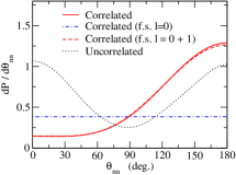
Figure 3: (Color online) The differential probability distribution with respect to the opening angle of the emitted two neutrons from ²⁶O. The solid and the dotted lines show the correlated and uncorrelated results, respectively. The dot-dashed and the dashed lines denote the correlated results obtained by including the angular momentum of the final state up to $l=0$ and $l=1$, respectively.

The angular distribution of the emitted neutrons can be also calculated using the decay amplitude, Eq. (5). The amplitude for emitting the two neutrons with spin components of $s_{1}$ and $s_{2}$ and momenta $\mbox{\boldmath$k$}_{1}$ and $\mbox{\boldmath$k$}_{2}$ reads EB92 ,

$$f_{s_{1}s_{2}}(\mbox{\boldmath$k$}_{1},\mbox{\boldmath$k$}_{2}) = \sum_{j,l}e^{-il\pi}e^{i(\delta_{1}+\delta_{2})}\,M_{j,l,k_{1},k_{2}}$$ (8)

$$\times\langle[{\cal Y}_{jl}(\hat{\mbox{\boldmath$k$}}_{1}){\cal Y}_{jl}(\hat{\mbox{\boldmath$k$}}_{2})]^{(00)}|\chi_{s_{1}}\chi_{s_{2}}\rangle,$$

where ${\cal Y}_{jlm}$ is the spin-spherical harmonics, $\chi_{s}$ is the spin wave function, and $\delta$ is the nuclear phase shift. The angular distribution is then obtained as

$$\frac{dP}{d\theta_{12}}=4\pi\sum_{s_{1},s_{2}}\int dk_{1}dk_{2}\,|f_{s_{1}s_{2}}(k_{1},\hat{\mbox{\boldmath$k$}}_{1}=0,k_{2},\hat{\mbox{\boldmath$k$}}_{2}=\theta_{12})|^{2},$$ (9)

where we have set $z$-axis to be parallel to $\mbox{\boldmath$k$}_{1}$ and evaluated the angular distribution as a function of the opening angle, $\theta_{12}$, of the two emitted neutrons.

The angular distribution obtained without including the final state $nn$ interaction is shown by the dotted line in Fig. 3. The main component in the initial wave function, $\Psi_{i}$, is the $d_{3/2}$ configuration, and the angular distribution is almost symmetric around $\theta_{12}=\pi/2$. In the presence of the final state $nn$ interaction, the angular distribution becomes highly asymmetric, in which the emission of two neutrons in the opposite direction (that is, $\theta_{12}=\pi$) is enhancedGMZ13 , as is shown by the solid line. Notice that we have obtained the correlated distribution by evaluating Eq. (9) only at $e_{1}+e_{2}=0.14$ and then normalize it, since it is hard to carry out the integrations in Eq. (9) when the resonance width is extremely small. We do not expect that this procedure causes any significant error in evaluating the angular distribution. The asymmetric angular distribution for the correlated case originates from the interference between opposite party components, as in the dineutron correlation in the density distribution CIMV84 . For the ²⁶O nucleus, it is due to the interference between the $l=0$ and $l=1$ components. The dot-dashed line in Fig. 3 shows the result obtained by including only $l=0$ in Eq. (8), while the dashed line shows the result with $l$=0 and 1. One can see that the angular distribution is almost exhausted by these two angular momenta and they contribute with almost equal amplitudes. For higher partial waves $l\geq 2$, the scattering wave functions in Eq. (6) are highly damped inside the centrifugal barrier since the energy is quite low ($e_{1}\sim e_{2}\sim$ 0.07 MeV). In other words, the two neutrons are rescattered into $s$-wave and $p$-wave states by multistep process due to the interaction $v$ (see Eq. (5)) and these low $l$ components uniquely enhance the penetrability, even though the main component in the initial wave function is the $d$-wave state. This picture is consistent with what Grigorenko et al. have argued in Ref.GMZ13 .

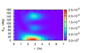
Figure 4: (Color online) The two-particle density for the resonance state of ²⁶O obtained with the box boundary condition. It is plotted as a function of $r_{1}=r_{2}=r$ and the angle between the valence neutrons, $\theta_{12}$.

The enhancement of angular distribution at backward angles for ²⁶O has also been seen theoretically in the dipole excitations of ¹¹Li EB92 and both theoretically and experimentally in the two-proton emission decay of ⁶Be G09 . This reflects the spatial correlation of the three-body resonance state of ²⁶O. Figure 4 shows the two-particle density for a resonance state of ²⁶O obtained with the box boundary condition as a function of $r_{1}=r_{2}=r$ and the opening angle between the two neutron, $\theta_{12}$. One finds that the density distribution is well localized in the small $\theta_{12}$ region, which is clear manifestation of the dineutron correlation HS05 . It has been well known that the configurations with opposite parity have to contribute coherently in order to form the dineutron correlation CIMV84 ; PSS07 ; HVPBS11 . In the angular distribution in Fig. 3, a phase factor, $e^{-il\pi}$, in the amplitude in Eq. (8) alters the sign of the contributions of odd partial waves, leading to the opposite tendency from the density, that is, the preference of emission of two-neutrons in the back-to-back angles. The nuclear phase shifts, $\delta_{1}+\delta_{2}$, plays a minor role in the decay of ²⁶O, partly because the decay energy is extremely small. Evidently, the back-to-back emission of two neutrons in the momentum space from the decay of ²⁶O is another manifestation of the strong dineutron correlation in the coordinate space of ground state density distribution.

For ¹⁶Be and ¹³Li, the experimental angular distributions show an enhancement of emission with relatively small opening anglesSKB12 ; KLD13 . It has yet to be clarified why these nuclei show different angular distributions from ²⁶O (and from ⁶Be and ¹¹Li). One possible reason is that the nuclear phase shift might play a more important role in these nuclei so that the phase factor $e^{-il\pi}$ is canceled out. Another reason may be the core excitation, with which the $nn$ configuration with coupled angular momenta of $J\neq 0$ is largely admixed in the ground state wave function. In order to confirm these points, three-body model calculations for these nuclei with the core excitations are clearly needed, but we leave them as a future work.

In summary, we have used the three-body model with a contact neutron-neutron interaction in order to analyze the two-neutron emission decay of the unbound neutron-rich nucleus ²⁶O. Using the Green’s function technique, we have analyzed the decay energy spectrum, the energy and the angular distributions of the two emitted neutrons. We have pointed out that the final state n-n interaction plays a crucial role to reproduce the strong low energy peak of the experimental decay energy spectrum. We have also argued that the energy distribution is a clear manifestation of a three-body resonance state and its density distribution is strongly reflected in the angular distribution of the emitted neutrons. In particular, the angular distribution clearly prefers the emission of the two neutrons in the back-to-back angles, that can be interpreted as a clear evidence for the dineutron correlation. So far, the energy and the angular distributions for the two-neutron decay of ²⁶O have not yet been measured experimentally. It would be extremely intriguing if they will be measured at new generation RI beam facilities, such as the SAMURAI facility at RIBF at RIKEN AN13 .

We thank Z. Kohley, T. Nakamura, A. Navin, Y. Kondo and T. Aumann for useful discussions. This work was supported by JSPS KAKENHI Grant Numbers 22540262 and 25105503.

References

- (1) C.A. Coulson and A.H. Neilson, Proc. Phys. Soc. 78, 831 (1961).
- (2) P. Rehmus, C.C.J. Roothaan, and R.S. Berry, Chem. Phys. Lett. 58, 321 (1978).
- (3) G.F. Bertsch, R.A. Broglia, and C. Riedel, Nucl. Phys. A91, 123 (1967).
- (4) F. Catara, A. Insolia, E. Maglione, and A. Vitturi, Phys. Rev. C28, 1091 (1984).
- (5) G.F. Bertsch and H. Esbensen, Ann. Phys. (N.Y.) 209, 327 (1991).
- (6) M.V. Zhukov et. al., Phys. Rep. 231, 151 (1993).
- (7) K. Hagino and H. Sagawa, Phys. Rev. C72, 044321 (2005).
- (8) M. Matsuo, K. Mizuyama, and Y. Serizawa, Phys. Rev. C71, 064326 (2005).
- (9) N. Pillet, N. Sandulescu, and P. Schuck, Phys. Rev. C76, 024310 (2007).
- (10) B. Walker et al., Phys. Rev. Lett. 73, 1227 (1994).
- (11) Th. Weber et al., Nature 405, 658 (2000).
- (12) B. Bergues et al., Nature Commun. 3, 813 (2012).
- (13) W. Becker, X.J. Liu, P.J. Ho, and J.H. Eberly, Rev. Mod. Phys. 84, 1011 (2012).
- (14) T. Nakamura et al., Phys. Rev. Lett. 96, 252502 (2006).
- (15) T. Aumann et al., Phys. Rev. C59, 1252 (1999).
- (16) T. Nakamura and Y. Kondo, Lec. Notes in Phys. 848, 67 (2012).
- (17) K. Hagino and H. Sagawa, Phys. Rev. C76, 047302 (2007).
- (18) C.A. Bertulani and M.S. Hussein, Phys. Rev. C76, 051602 (2007).
- (19) H. Esbensen and G.F. Bertsch, Nucl. Phys. A542, 310 (1992).
- (20) K. Hagino, H. Sagawa, T. Nakamura, and S. Shimoura, Phys. Rev. C80, 031301(R) (2009).
- (21) Y. Kikuchi et al., Phys. Rev. C81, 044308 (2010).
- (22) M. Pfützner, M. Karny, L.V. Grigorenko, and K. Riisager, Rev. Mode. Phys. 84, 567 (2012), and references therein.
- (23) A. Spyrou et al., Phys. Rev. Lett. 108, 102501 (2012).
- (24) H.T. Johansson et al., Nucl. Phys. A842, 15 (2010); Nucl. Phys. A847, 66 (2010).
- (25) Yu. Aksyutina et al., Phys. Lett. B666, 430 (2008).
- (26) E. Lunderberg et al., Phys. Rev. Lett. 108, 142503 (21012).
- (27) C. Caesar et al., arXiv:1209.0156.
- (28) Z. Kohley et al., Phys. Rev. C87, 011304(R) (2013).
- (29) F.M. Marqués et al., Phys. Rev. Lett. 109, 239201 (2012).
- (30) H. Esbensen, G.F. Bertsch, and K. Hencken, Phys. Rev. C56, 3054(1997).
- (31) B. Jurado et al., Phys. Lett. B649, 43 (2007).
- (32) C.R. Hoffman et al., Phys. Rev. Lett. 100, 152502 (2008).
- (33) T. Otsuka et al., Phys. Rev. Lett. 95, 232502 (2005); Phys. Rev. Lett. 105, 032501 (2010).
- (34) Fl. Stancu, D.M. Brink, and H. Flocard, Phys. Lett. 68B, 108 (1977).
- (35) G. Colo, H. Sagawa, S. Fracasso, and P.F. Bortignon, Phys. Lett. B646, 227 (2007).
- (36) T. Lessinski et al., Phys. Rev. C76, 014312 (2007).
- (37) Z. Kohley et al., Phys. Rev. Lett. 110, 152501 (2013).
- (38) L.V. Grigorenko, I.G. Mukha, and M.V. Zhukov, Phys. Rev. Lett. 111, 042501 (2013).
- (39) L.V. Grigorenko et al., Phys. Rev. C80, 034602 (2009).
- (40) K. Hagino, A. Vitturi, F. Perez-Bernal, and H. Sagawa, J. of Phys. G38, 015105 (2011).
- (41) T. Aumann and T. Nakamura, Phys. Scr. T152, 014012 (2013).