Pseudopotential model for Dirac electrons in graphene with line defects

Abstract

We consider electron transport in a planar fermion model containing various types of line defects modelled by $\delta$–function pseudopotentials with different matrix coefficients. The transmission probability for electron transport through the defect line is obtained for various types of pseudopotentials. For the schematic model considered that may describe a graphene structure with different types of linear defects, the valley polarization is obtained.

Key words: Low dimensional models; Line defect; Valley polarization; Graphene.

I Introduction

For the last years special interest in 2+1 dimensional models appears in condensed matter physics. An important prototype of such models is graphene Novos , 1 , 2 , a planar monoatomic layer of carbon, which may be regarded as a superposition of two triangular sublattices, $A$ and $B$, forming a hexagonal lattice. As it has been recently discovered, graphene posesses various unusual properties. For instance, in Geim10 , Geim0 such properties as anomalous Hall effect, conductivity and other interesting features of material were investigated. The behavior of electrons in problems related to graphene can be effectively described by the Dirac equation for massless fermions obtained from a continuum version of the tight-binding model wallace , Semenoff , Gus , Neto2 . A chiral gauge theory for graphene was formulated in jackiw . Further studies of the theory of two-dimensional tight-binding quantum systems, as described in the continuum approximation by the Dirac equation in (2+1)-dimensional space-time with account for topological properties, were made in Hou ,Chamon , Obispo . Note that, despite its similarity, this equation is in this context not a relativistic wave equation, but arises by linearizing the energy as a function of a momentum near Dirac points, i.e. intersections of the energy dispersion with the Fermi level.

Recently, models with different types of defects in the structure of planar systems have attracted much attention. These defects can lead to many nontrivial properties of the transmission of propagating particles, which are related to nonuniform densities near the defects and barriers. Recent investigations in graphene provide various examples of this kind of problems. Let us mention, in particular, the recently observed topological line defect, containing the periodic repetition of one octagonal plus two pentagonal carbon rings along a certain direction embedded in a perfect graphene sheet Lahiri , and also interesting grain boundaries Huang in graphene. Clearly, more new important applications of low-dimensional structures can be realized, when transport problems in them are well understood. In particular, as line defects have a simple geometry, this makes them easier for a theoretical study and suitable for the use for controlled transport in graphene. In this context, let us mention the recent theoretical studies of electronic transport through a line defect in graphene considered in China2 , which were based upon the Green function approach.

The aim of this paper is to study line defects as barriers for the electron propagation by using the effective Dirac equation for massless electrons in (monolayer) graphene wallace ; Semenoff ; Gus ; Geim10 ; Geim0 , in the framework of a schematic pseudopotential model. We shall consider all possible types of barrier-type perturbations, chosen for convenience at the same position $x$ and described in the limiting case by a pseudopotential term $W(x)$, depending on pseudospin (sublattice) indices and valley (Dirac point) indices. In this way, the problem of describing line defects in planar systems can be mapped to a delta-function pseudopotential $W(x)=W\delta(x)$, and this helps us to find exact analytic solutions in a simple way. Note, in particular, that the pseudopotentials in the form of delta-function barriers with Pauli- matrix coefficients, mimicking the pseudospin and valley structure of the defect line, will be considered as limiting cases of induced gauge fields arising due to perturbations in the hopping parameters Geim0 , Neto2 , Vozmediano .

II Pseudopotential for the effective 2D Dirac equation

Consider a planar system modeling monolayer graphene with electrons in $D=2+1$ space-time. Different physical mechanisms give rise to (perturbative) interaction terms in the effective Dirac Hamiltonian that describes electrons in graphene. These perturbations may arise due to several types of disorder, like topological lattice defects, strains, and curvature. Such defects are expected to exist in graphene, as experiments show a significant corrugation both in suspended samples, in samples deposited on a substrate, and also in samples grown on metallic surfaces (see, e.g., Vozmediano , Guinea , and references therein). Note, in particular, that changes in the distance between the atoms and in the overlap between the different orbitals by strain or bending lead to changes in the nearest–neighbor ($NN$) hopping or next–nearest– neighbor ($NNN$) hopping amplitude and this results in the appearance of vector potentials $A_{x}(\vec{r})$, $A_{y}(\vec{r})$ (this coupling must take the form of a gauge field with the matrix structure of the Pauli matrices, $\sigma_{1}$ and $\sigma_{2}$) and a scalar potential $V(\vec{r})$ in the Dirac Hamiltonian Geim0 ,Neto2 ,Vozmediano . Moreover, in a region of finite mass the Hamiltonian for Dirac electrons should include a ${\vec{r}}-$dependent mass term $t^{\prime}=v^{2}_{F}m({\vec{r}})$ ($m({\vec{r}})$ is the effective mass with a $\sigma_{3}$ matrix) due to which the electronic spectrum will obtain a finite energy gap. Practically, this type of term can be generated by covering the surface of graphene with gas molecules gas1 , or by depositing graphene on top of boron nitride gas2 ; gas3 .

Let us therefore start with the following general expression for the Hamiltonian including the induced gauge potentials and a mass term

$${\cal H} = \sum_{\tau=\pm 1}\int d^{2}x\Psi^{{\dagger}}_{\tau}(\vec{r})\left\{\sigma_{1}\left[-v_{\rm F}\ i\partial_{x}-A_{x}(\vec{r})\right]+\tau\sigma_{2}\left[-v_{\rm F}i\partial_{y}-A_{y}(\vec{r})\right]\right\}\Psi_{\tau}(\vec{r})+$$ (1)

$$+ \sum_{\tau=\pm 1}\int d^{2}x\Psi_{\tau}^{{\dagger}}(\vec{r})\left[t^{\prime}(\vec{r})\sigma_{3}+V(\vec{r})\,\,\,I\right]\Psi_{\tau}(\vec{r}).$$

Here the spinors in the 2D plane $\Psi_{\tau}(\vec{r})$ ($\tau=\pm 1$, $\vec{r}=(x,\,\,y)$) have two components

$$\Psi_{\tau}(\vec{r})=\begin{pmatrix}\Psi_{1,\tau}\\ \Psi_{2,\tau}\\ \end{pmatrix}$$ (2)

describing electrons at the two $A,\,\,B$ sublattices ($i=1,2$); $\sigma_{i}$ are $2\times 2$ Pauli-matrices, $I$ is the unit matrix and $v_{F}$ is the Fermi velocity .

The physical spin of the electrons that is due to spatial rotation properties of the electron wavefunction has been neglected in our analysis, and the spinor nature of the wavefunction has its origin in the sublattice degrees of freedom called pseudospin. The subscript $\tau=\pm 1$ stands for the two Fermi points $K,\,\,K^{\prime}$, corresponding to valleys at the corners in the first Brillouin zone and plays the role of a flavor index. Besides the above effective gauge fields an effective electrostatic potential barrier may also influence the electron propagation in graphene (see, e.g., Geim2 ). The term that is responsible for this (and equally magnetic) interaction may be included in the Hamiltonian just as an electrostatic scalar potential $e\Phi(\vec{r})$ (and vector potential $e{\vec{A}_{elm}}$). The corresponding property of “relativistic” Dirac electrons in graphene is their ability to tunnel through such a potential barrier with probability one. This is the so called Klein tunneling of chiral particles (see, e.g., Geim2 ). Its presence in graphene is undesirable for graphene applications to nanoelectronics. In order to overcome this difficulty, one may generate a gap in the spectrum, which is equivalent to the generation of a spatial-dependent mass term. Clearly, the simultaneous existence of a scalar potential barrier and a vector gauge field ${\vec{A}}=(A_{x},\,\,A_{y})$ at some spatial regions may influence the electron transmission, say in the $x-$direction. In order to study the possible joint role and competition of these perturbations, we combined them in the model Hamiltonian (1).

In this way, we assume that the motion of electrons is described by the planar Dirac equation $H_{\tau}\Psi_{\tau}=i\partial_{t}\Psi_{\tau}$ with the Dirac Hamiltonian operator

$$H_{\tau} = \sigma_{1}\left[-v_{\rm F}i\partial_{x}-A_{x}(\vec{r})\right]+$$ (3)

$$+ \tau\sigma_{2}\left[-v_{\rm F}i\partial_{y}-A_{y}(\vec{r})\right]+v_{\rm F}^{2}m(\vec{r})\sigma_{3}+V(\vec{r})\,\,\,I,$$

where $\tau=\pm 1$ is the valley index. The expression Eq.(3) implies that the low-momentum expansion around the other Fermi point with $\tau\to-\tau$ gives rise to a time-reversed Hamiltonian. Note that the total effect of both valleys, as described in 4-spinor notations Gus (and references therein), respects time-reversal invariance. Let us now assume that the considered possible defects are lying in the same spatial region taken, for simplicity, to have the form of a line lying on the y-axis($x=0$). So our study is considered as investigation of a delta-function limit of more realistic barrier-type configurations and may be based on the schematic model Hamiltonian

$$H_{\tau}=-i\sigma_{1}\partial_{x}-i\tau\sigma_{2}\partial_{y}+W_{\tau}(x),$$ (4)

where we have introduced the pseudopotential $W_{\tau}(x)$

$$W_{\tau}(x)=V(x)I-A_{x}(x)\sigma_{1}-\tau A_{y}(x)\sigma_{2}+m(x)\sigma_{3},$$ (5)

which in a delta-function limit can be written in the form

$$W_{\tau}(x)=W_{\tau}\delta(x)=(aI-b_{1}\sigma_{1}-b_{2}\tau\sigma_{2}+b_{3}\sigma_{3})\delta(x).$$ (6)

In Eq.(4), and in what follows, the Fermi velocity, with the corresponding choice of the units, is supposed to be equal to unity, $v_{F}=1$. The scalar and vector potentials and the mass-type term are chosen as $V(x)=a\delta(x),\,\,A_{x}=b_{1}\delta(x),\,\,A_{y}=b_{2}\delta(x)$, $m(x)=b_{3}\delta(x)$, where $a,\,\,b_{i}\,\,(i=1,2,3)$ are constants that describe the interactions of particles in sublattices from either side of the line defect and are related to “hopping parameters” (see in what follows).

Let us now apply the above schematic model to graphene with line defects, arising in the form of deformations in the structure or displacements of carbon atoms of the hexagonal crystal lattice (some of these defects were e.g. described in gun ; china ).

The (2+1)-dimensional Dirac equation for the model under consideration

$$\left[i\partial_{t}+i\sigma_{1}\partial_{x}-\tau\sigma_{2}p_{y}-W_{\tau}\delta(x)\right]\Psi_{\tau}=0$$ (7)

has stationary solutions

$$\Psi_{\tau}(\vec{r},t)=\begin{pmatrix}\Psi_{1,\tau}\\ \Psi_{2,\tau}\\ \end{pmatrix}e^{ip_{y}y}e^{-iEt},$$ (8)

where the functions $\Psi_{i,\tau}(x),\,\,(i=1,2)$ should be found by a limiting procedure around the defect line $x=0$. The solutions of the free Dirac equation for $\tau=+1$ (for $\tau=-1$ the corresponding solution is also easily found) in the $x<0$ and $x>0$ regions can be written respectively as (to simplify notations, we omit here the subscript $\tau=+1$)

$$\begin{pmatrix}\Psi_{1}\\ \Psi_{2}\end{pmatrix}_{<}=\begin{pmatrix}1\\ \mathop{\rm e}\nolimits^{i\beta}\end{pmatrix}\mathop{\rm e}\nolimits^{ip_{x}x}+B\begin{pmatrix}1\\ -\mathop{\rm e}\nolimits^{-i\beta}\end{pmatrix}\mathop{\rm e}\nolimits^{-ip_{x}x},$$ (9)

$$\begin{pmatrix}\Psi_{1}\\ \Psi_{2}\end{pmatrix}_{>}=C\begin{pmatrix}1\\ \mathop{\rm e}\nolimits^{i\beta}\end{pmatrix}\mathop{\rm e}\nolimits^{ip_{x}x},$$ (10)

where $\beta$ is the incident angle of the electron wave with respect to the x-axis, $p_{x}=p\cos\beta,\,\,\,p_{y}=p\sin\beta$.

III Transmission through the pseudopotential

Let us next study the transmission through the defect line in two particular cases of main interest:
1) $b_{1}\neq 0,\,\,a=b_{2}=b_{3}=0$, and 2) $b_{1}=0$, $a\neq 0,\,\,b_{2}\neq 0,\,\,b_{3}\neq 0$.

III.1 $b_{1}\neq 0,\,\,a=b_{2}=b_{3}=0$

The Dirac equations now take the form

$$\left\{\begin{array}[]{l}E\Psi_{1}+i\Psi^{{}^{\prime}}_{2}+i\tau p_{y}\Psi_{2}+b_{1}\delta(x)\Psi_{2}=0,\\ E\Psi_{2}+i\Psi^{{}^{\prime}}_{1}-i\tau p_{y}\Psi_{1}+b_{1}\delta(x)\Psi_{1}=0,\\ \end{array}\right.$$ (11)

where $\Psi_{i}^{\prime}=d\Psi_{i}/dx$.

Multiplying the first equation by $\Psi_{1}$, the second by $\Psi_{2}$ and then, in order to exclude the $\delta-$function, subtracting the equations we obtain

$$E(\Psi_{1}^{2}-\Psi_{2}^{2})+i(\Psi_{1}\Psi_{2}^{{}^{\prime}}-\Psi_{2}\Psi_{1}^{{}^{\prime}})+2i\tau p_{y}\Psi_{1}\Psi_{2}=0.$$ (12)

Dividing this equation by $\Psi_{1}^{2}$, integrating over $x$ between $-\varepsilon$ and $+\varepsilon$ ($\varepsilon\rightarrow 0$) and assuming that the discontinuities of the functions are finite, we find the first boundary condition

$$\left.\frac{\Psi_{2}}{\Psi_{1}}\right|^{+\varepsilon}_{-\varepsilon}=0.$$ (13)

Now divide the first equation in (11) by $\Psi_{2}$, the second by $\Psi_{1}$, and integrate both equations over $x$ between $-\varepsilon$ and $+\varepsilon$ ($\varepsilon\rightarrow 0$). The new boundary conditions look like

$$\left\{\begin{array}[]{l}\left.i\log(\Psi_{2})\right|^{+\varepsilon}_{-\varepsilon}=-b_{1},\\ \left.i\log(\Psi_{1})\right|^{+\varepsilon}_{-\varepsilon}=-b_{1}.\\ \end{array}\right.$$ (14)

Upon substitution of the solution for the free Dirac equation (9) and (10) in (13), (14), the transmission probability for both values of the valley indices $\tau=\pm 1$ is found to be equal to unity

$$T_{\sigma_{1}}=|C|^{2}=1.$$ (15)

This result can easily be explained from the point of view of the graphene structure. In the two-dimensional graphene model the spinor basis can be written in the form $\Psi_{\tau}=\begin{pmatrix}\Psi_{1,\tau}\\ \Psi_{2,\tau}\\ \end{pmatrix},$ where $\Psi_{1,\tau},\Psi_{2,\tau}$ are related to the $A,B$ sublattices of graphene. The $\sigma_{1}$ matrix in front of the $\delta(x)$–function in the Dirac equation interchanges the $A$ and $B$ sublattice components in the wave function. However in the tight-binding model of graphene one sums all terms over one sublattice, either $A$ or $B$ and the corresponding nearest neighbors of the other sublattice, so that the graphene model is invariant under the transformation $A\to B,\,\,B\to A$. By this reason, the incident wave propagates without any reflection, since in this case the potential $-b_{1}\delta(x)\sigma_{1}$ does not form any barrier for it.

III.2 $b_{1}=0$, $a\neq 0,b_{2}\neq 0,b_{3}\neq 0$

Consider the more general case with $a,b_{2},b_{3}\neq 0$, and only $b_{1}=0$. The Dirac equation (7) now takes the form

$$\left[E+i\sigma_{1}\partial_{x}-\tau\sigma_{2}p_{y}-\delta(x)(aI-b_{2}\tau\sigma_{2}+b_{3}\sigma_{3})\right]\Psi_{\tau}=0,$$ (16)

which transforms to the set of equations (omitting the index $\tau$ in the wave function)

$$\left\{\begin{array}[]{l}E\Psi_{1}+i\Psi^{{}^{\prime}}_{2}+i\tau p_{y}\Psi_{2}-\delta(x)(a\Psi_{1}+i\tau b_{2}\Psi_{2}+b_{3}\Psi_{1})=0,\\ E\Psi_{2}+i\Psi^{{}^{\prime}}_{1}-i\tau p_{y}\Psi_{1}-\delta(x)(a\Psi_{2}-i\tau b_{2}\Psi_{1}-b_{3}\Psi_{2})=0.\\ \end{array}\right.$$ (17)

After performing some further transformations and subsequent integration in the above equations to avoid problems with the delta-function (analogously to what has been done in the previous Section), we arrive at the expression

$$\left.{1\over N}\arctan\left[\frac{1}{N}\left((a+b_{3})\frac{\Psi_{1}}{\Psi_{2}}+i\tau b_{2}\right)\right]\right|^{+\varepsilon}_{-\varepsilon}=i,$$ (18)

where $N=\sqrt{b_{3}^{2}+b_{2}^{2}-a^{2}}$.

Substituting $\frac{\Psi_{1}}{\Psi_{2}}$ with the wave functions $\Psi_{i}(x=\pm\varepsilon)$ from Eqs. (9) and (10), we find the transmission probability for both values of the valley index $\tau=\pm 1$

$$T_{I,\sigma_{2},\sigma_{3}}(\tau)=|C|^{2}=1-|B|^{2}=\frac{1}{\cosh^{2}N}\,\,\frac{\cos^{2}\beta}{\cos^{2}\beta+\frac{(a-b_{2}\tau\sin\beta)^{2}}{b_{3}^{2}+b_{2}^{2}-a^{2}}\tanh^{2}N}.$$ (19)

For a beam of electrons propagating towards the line defect, the scattered electrons will now be valley-polarized. The valley polarization being defined as Gun2

$$P_{\tau}=\frac{T_{(\tau=+1)}-T_{(\tau=-1)}}{T_{(\tau=+1)}+T_{(\tau=-1)}},$$ (20)

thus takes the form

$$P_{\tau}=\frac{2ab_{2}\sin\beta\tanh^{2}N}{\cos^{2}\beta(b_{3}^{2}+b_{2}^{2}-a^{2})+(a^{2}+b_{2}^{2}\sin^{2}\beta)\tanh^{2}N}.$$ (21)

As can be seen from the above formula, the valley polarization becomes equal to zero for the incident angle $\beta=0$.

III.3 Comparison with other models

It is instructive to compare the results of the previous Subsection, where we have admitted three matrix coefficients in front of the $\delta(x)$-function, $I,\sigma_{2},\sigma_{3}$, with some special cases considered in the literature.

1. Scalar potential barrier Geim2

Clearly, the unit matrix $I$ in Eqs. (1), (6), corresponds to diagonal pseudospin transitions $A\to A,\,\,B\to B$ with respect to the defect line, i.e. the graphene to the left of the defect line is mirror symmetric to the graphene on the right side of the defect line. This corresponds, e.g., to the model of graphene with a scalar (electrostatic) potential barrier of rectangular shape considered in Ref. Geim2

$$V(x)=\left\{\begin{array}[]{l}V_{0},0<x<D\\ 0,{\rm otherwise}\\ \end{array}\right..$$ (22)

The authors of Geim2 obtained the transmission probability for this model

$$T_{D}=\frac{\cos^{2}\beta}{1-\cos^{2}(q_{x}D)\sin^{2}\beta},$$ (23)

where $q_{x}=\sqrt{(E-V_{0})^{2}/\hbar^{2}v^{2}_{F}-k^{2}_{y}}$. Note that, in the limit $D\to 0,\,\,V_{0}\to\infty$, $q_{x}D<\infty$, where $D$ and $V_{0}$ are the potential barrier width and height, this result goes over to our expression (19) for the transmission probability for a delta-barrier, if we put $b_{2}=b_{3}=0,a\neq 0$, with $q_{x}D=a$

$$T_{a}=\frac{\cos^{2}\beta}{1-\cos^{2}a\sin^{2}\beta}.$$ (24)

2. Defect line containing pentagonal and octagonal carbon rings Lahiri ; China2

Let us next consider the model of graphene with a defect line, containing pentagonal and octagonal carbon rings, described, e.g. in Lahiri ; gun ; china ; China2 . In China2 the authors with the use of the tight-binding lattice model and the Green function formalism obtained the following result for the transmission probability in the low energy limit

$$T_{(\tau=\pm 1)}=\frac{\tau_{1}^{4}\cos^{2}\beta}{(\tau_{1}^{4}+\tau_{2}^{2})\mp 2\tau_{1}^{2}\tau_{2}\sin\beta},$$ (25)

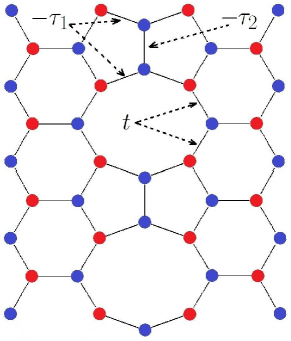
Figure 1: Line defect, consisting of the periodic repetition of one octagonal and two pentagonal carbon rings. Red circles correspond to sublattice A, blue circles to sublattice B; $t$, $-\tau_{1}$, $-\tau_{2}$ are NN-hopping energies.

where $\tau_{1},\,\,\tau_{2}$ are NN-“hopping parameters” (see Fig.1). Using the notation of the authors $x=\tau_{2}/\tau_{1}^{2}$, one can rewrite (25) as follows

$$T_{(\tau=\pm 1)}=\frac{\cos^{2}\beta}{(1+x^{2})\mp 2x\sin\beta}.$$ (26)

To compare this expression with our results, let us consider Eq.(19) in the particular case, when $b_{3}=0$, i.e. when the effective mass-type term is neglected. There arises an interesting structural similarity with (26), if the parameters $a$, $b_{2}$ of diagonal and non-diagonal pseudospin interactions in the pseudopotential (6) are not taken independently, but are assumed to satisfy the following relation

$$\frac{b^{2}_{2}}{a^{2}}=\cosh^{2}(N),$$ (27)

where now $N=\sqrt{b^{2}_{2}-a^{2}}$. By inserting (27) into the expression (19) and putting $b_{3}=0$, we obtain in the framework of our schematic model

$$T_{I,\sigma_{2}}=\frac{\cos^{2}\beta}{\cosh^{2}(N)\left[(1+\frac{a^{2}}{b_{2}^{2}})-2\tau\frac{a}{b_{2}}\sin\beta\right]}=\frac{\cos^{2}\beta}{(1+\frac{b_{2}^{2}}{a^{2}})-2\tau\frac{b_{2}}{a}\sin\beta}.$$ (28)

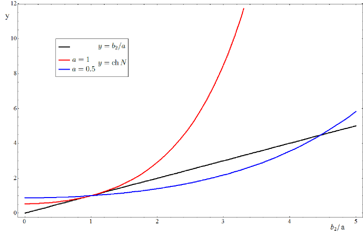
Figure 2: Solution of the equation $\frac{b_{2}}{a}=\cosh{}N$ (see (27) in the text) for different values of $a$.

It should be noted that Eq. (27) has besides the trivial solution $\frac{b_{2}}{a}=1$, a nontrivial solution for the ratio $\frac{b_{2}}{a}\neq{}1$, if $a<1$. This can be seen from Fig.2. It is clear that for $a\geq 1$ there exists only the trivial solution $\frac{b_{2}}{a}=1$, and the transmission probability can reach in this case its maximum value $T_{I,\sigma_{2}}=1$ for $\beta=\pm{\pi\over 2}$ ($\tau=\pm 1$).

It is amazing to note that our result (28) indeed looks similar to the expression (26), derived in paper China2 as a low energy limit in a much more involved calculation. By identifying the expressions $b_{2}/a=\tau_{2}/\tau_{1}^{2}=x$, it thus could be suggested that the coefficients $a$, $b_{2}$ in our pseudopotential model effectively correspond to the hopping parameter quantities $\tau_{1}^{2}$, and $\tau_{2}$, respectively. This way, one may conclude that $a$ mimics the $NNN$ diagonal pseudospin transitions of electrons via two neighboring pentagons of the linear defect in Fig. 1, giving $\tau_{1}$-hopping squared, whereas $b_{2}$ is responsible for $NN$-hopping between two mismatched atoms of the B sublattice corresponding to $\tau_{2}$. Obviously, such a correspondence between $a$, $b_{2}$ and $\tau_{1}^{2}$, and $\tau_{2}$ supports the original interpretation of the role of these interactions in the pseudopotential (6) and looks like a concrete realization of the ideas of Geim0 , Vozmediano , where the “scalar potential” term $a\delta(x)$ mimics the $NNN$ hopping, while the “vector-potential” term $b_{2}\sigma_{2}\delta(x)$ mimics the $NN$-hopping. Note that the above application and interpretation of the pseudopotential method required an important additional input: namely, the specific parameter relation Eq.(27) which apparently in some effective way reflects the internal microscopic structure of the defect line. Clearly, such an approach can offer only an approximate qualitative description of transmission phenomena.

IV Numerical results

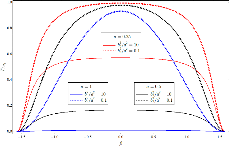
Figure 3: Transmission probability $T$ in dependence of the angle of incidence $\beta$ for $b_{2}=0$ and for different values of parameter $a$ and ratio $b_{3}^{2}/a^{2}$.

Let us now return to the expressions for the transmission probability (19) and the valley polarization (21) of our schematic model for the case with $a\neq 0$ and $b_{3}\neq 0$ simultaneously. The corresponding result could be useful for future researches, because the transmission probability has a nontrivial behavior (see Fig. 3) and the valley polarization (21) equals zero only for zero incident angle $\beta=0$.

The dependence of the transmission on the angle of incidence in the case $b_{2}=0$, $a\neq 0$, $b_{3}\neq 0$ is as follows

$$T_{I,\sigma_{3}}=\frac{\cos^{2}\beta}{\cosh^{2}(a\sqrt{b^{2}_{3}/a^{2}-1})\cos^{2}\beta+\sinh^{2}(a\sqrt{b^{2}_{3}/a^{2}-1})\frac{1}{b^{2}_{3}/a^{2}-1}}.$$ (29)

Its behavior is shown in Fig.3. Obviously, if the contribution of the coefficient $b_{3}$ is greater than that of the coefficient $a$ the transmission is lower. However, if the contribution of the coefficient $b_{3}$ is lower than that of the coefficient $a$ for the same values of $a$, the transmission probability increases. As follows from Eq. (29), it can reach for values of $a\gg b_{3}$ the value $T=1$ (for $\beta=0$) (see Fig. 3).

As is known gas3 ; Guinea , the term in the D=(2+1) Hamiltonian (3) of the model with the $\sigma_{3}$ matrix corresponds to the effective mass of electrons, and as a consequence the electronic spectrum will present a finite energy gap. The existence of an energy gap prevents the Klein paradox from taking place, a necessary condition for building nanoelectronic devices made of graphene. Our conclusion supports the results of the authors of gas3 ; Guinea about the role of the mass term as a factor impeding the Klein tunnelling of chiral electrons through the barrier. The valley polarization for the case $\beta=0$ is still equal to zero. It should also be noted that our result (19), (29) for the transmission probability in the case with only $b_{3}\neq 0$ corresponds to that of paper gas3 in the limiting case of a narrow region with finite mass

$$T_{\sigma_{3}}(\tau)=|C|^{2}=1-|B|^{2}=\frac{1}{\cosh^{2}N},\,\,\,N=|b_{3}|.$$ (30)

Obviously, in the case $a=0$ the valley polarization (21) equals zero at any angle, and the dependence of the transmission probability on the angle of incidence is described by the formula

$$T_{\sigma_{2},\sigma_{3}}=\ \frac{\cos^{2}\beta}{\cosh^{2}(b_{2}\sqrt{b^{2}_{3}/b_{2}^{2}+1})\cos^{2}\beta+\sinh^{2}(b_{2}\sqrt{b^{2}_{3}/b_{2}^{2}+1})\frac{\sin^{2}\beta}{b^{2}_{3}/b_{2}^{2}+1}}.$$ (31)

The interesting result in this case is that the transmission is lower, if the coefficient $b_{3}$ is greater than the coefficient $b_{2}$ (see Fig. 4 for various values of $b_{2}$).

The third case corresponds to graphene with a defect line for $a\neq 0,\,\,b_{2}\neq 0$ gun ; china ; China2 . It follows from our general result (19) that

$$T_{I,\sigma_{2}}=\frac{\cos^{2}\beta}{\cosh^{2}(a\sqrt{b^{2}_{2}/a^{2}-1})\cos^{2}\beta+\sinh^{2}(a\sqrt{b^{2}_{2}/a^{2}-1})\frac{(1-(b_{2}/a)\tau\sin\beta)^{2}}{b^{2}_{2}/a^{2}-1}}.$$ (32)

The transmission is still higher for small values of $a$, and the maximum of transmission for the case $a\simeq{}b_{2}$ is observed for the angles $\beta\rightarrow\pi/2$, and for the angles $\beta\rightarrow-\pi/2$, $(\tau=+1)$ (see Fig. 5a)). If the contributions of the coefficients $a$ and $b_{2}$ are not equal ($a\gg{}b_{2}$ or $a\ll{}b_{2}$), the maximum of the transmission probability is shifted from the angles $\beta\simeq\pm\pi/2$ towards the center of the graph. It should be noted, that the transmission probability for the case $a\ll{}b_{2}$ is small, while for the case $a\gg{}b_{2}$ it tends to $1$ in its maximum for any values of $a$ (see Fig. 5b)). The valley polarization for this case is given in (21), if we set $b_{3}=0$. The result for $a>1$ is similar to that of paper Gun2 (see Fig. 6 black line). The polarization for $a\simeq 1$ has an almost linear dependence on the angle $\beta$ (see Fig. 6 red line). However for $a<1$ the dependence of the valley polarization on the angle of incidence has a nontrivial behavior (see Fig. 6 blue line). The graphics of the valley polarization for different contributions of the coefficients $a,b_{2}$ for the same values of $a$ are shown in Fig. 7a),b).

V Summary and conclusions

In this paper, we have studied a planar electron system for graphene containing a defect line with a pseudospin and valley structure by using a schematic model with a delta-function pseudopotential. The underlying structure of the considered pseudopotential is assumed to arise from various perturbations on the line, in particular strain, which lead to changes in the $NN$ and $NNN$ hopping amplitudes and are represented by vector and scalar gauge fields with the matrix structure of the sublattice (pseudospin) Pauli matrices and the unit matrix in the Dirac Hamiltonian. In addition, a space-dependent mass term, localized in a narrow region of space, was taken into account and described by including a delta-function term with a $\sigma_{3}$ matrix coefficient. On this basis, the transmission through a defect line in the graphene structure with various pseudospin types of defects was considered, and the transmission probability and valley polarization were obtained in the framework of the considered schematic model. Moreover, we presented also justifications for dealing with a $\delta$–function pseudopotential as a model of a narrow square barrier by considering limiting cases of special interest. Note that in the limit of a narrow square barrier our calculation proved to be in agreement with the corresponding limit of the result of Geim2 obtained for the electrostatic potential barrier of finite width (Klein paradox). Moreover, the considered pseudopotential model allows also an interesting effective description of a defect line with linear repetition of two pentagonal and one octagonal carbon rings (Lahiri ; China2 ). In particular, it was shown that our results go over to those obtained earlier on the basis of the Green function method (China2 ), if the parameters $a$, $b_{2}$ of diagonal and non-diagonal pseudospin interactions in the pseudopotential (6) are not taken independently, but are assumed to satisfy the specific relation (27).

We hope that the considered pseudopotential method and results of this paper may help to enlarge, at least qualitatively, our understanding of the transport problems of charged particles in planar configurations containing line defects with various pseudospin structures.

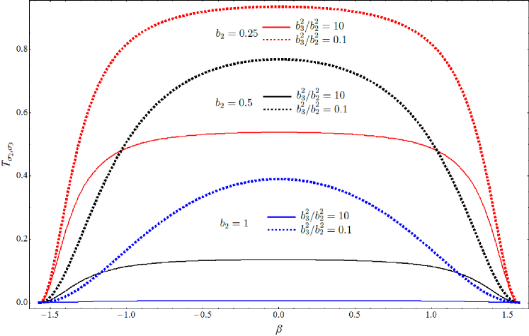
Figure 4: Transmission probability $T$ for $a=0$ and for different values of the parameter $b_{2}$ and ratio $b_{3}^{2}/b_{2}^{2}$.

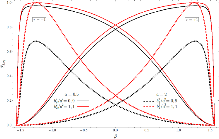
a)

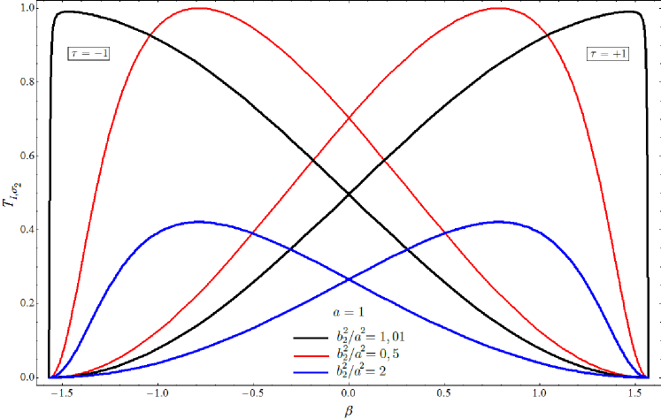
b)

Figure 5: Transmission probability $T$ for different valley indices $\tau=\pm 1$ as a function of the incident angle $\beta$ for $b_{3}=0$ and for different values of the parameter $a$ and ratio $b_{2}^{2}/a^{2}$.

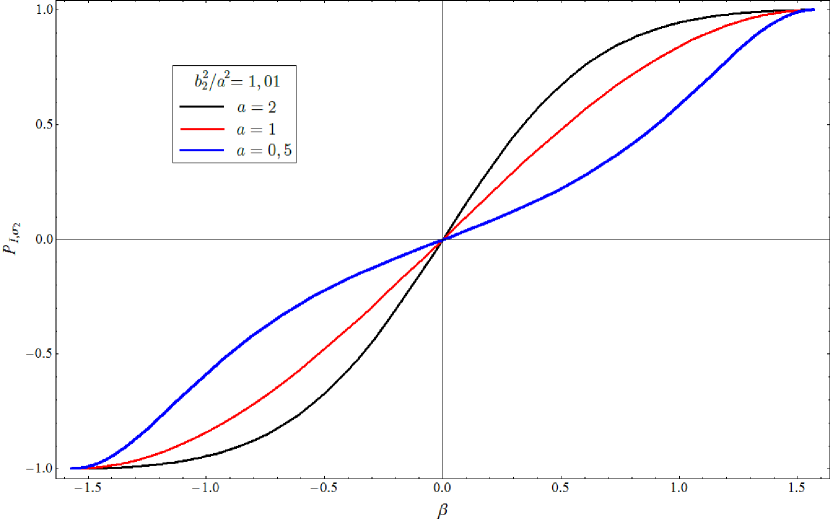
Figure 6: Valley polarization $P$ as a function of the angle of incidence $\beta$ for $b_{3}=0$ and $b_{2}^{2}/a^{2}=1.01$ for different values of the parameter $a$.

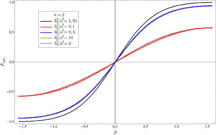
a)

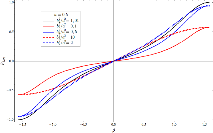
b)

Figure 7: Valley polarization $P$ as a function of the angle of incidence $\beta$ for $b_{3}=0$ and for different values of the parameter $a$ and ratio $b_{2}^{2}/a^{2}$.

References

- (1) K.S. Novoselov, A.K. Geim, S.V. Morozov, D.Jiang, Y.Zhang, S.V. Dubonos, I.V. Grigorieva, and A.A. Firsov, Science 306, 666 (2004).
- (2) M.I. Katsnelson, Mater. Today, 10, 20 (2007).
- (3) A.K. Geim, Science, 324, 1530 (2009).
- (4) K.S. Novoselov, A.K. Geim, S. V. Morozov, D. Jiang, M. I. Katsnelson, I. V. Grigorieva, S. V. Dubonos and A. A. Firsov, Nature 438, 197 (2005).
- (5) A.H. Castro Neto, F. Guinea, N. M. R. Peres, K. S. Novoselov and A. K. Geim Rev. Mod. Phys. 81, 109 (2009).
- (6) P.R. Wallace, Phys. Rev. 71, 622 (1947).
- (7) G.W. Semenoff Phys. Rev. Lett, 53, 2449 (1984).
- (8) V.P. Gusynin, S.G. Sharapov, and J.P. Carbotte, Int. J. Mod. Phys., B21, 4611 (2007).
- (9) A. H. Castro Neto, ArXiv: 1004.3682 [cond-mat.mtrl-sci]
- (10) R. Jackiw and S.-Y. Pi, Phys. Rev. Lett. 98, 26402 (2007).
- (11) C. Chamon, C.-Yu Hou, R. Jackiw, C. Mudry, S.-Y. Pi, and A.P. Schnyder, Phys. Rev. Lett., 100, 110405 (2008).
- (12) C. Chamon, C.-Yu Hou, R. Jackiw, C. Mudry, S.-Y. Pi and G.Semenoff, Phys. Rev.B, 77, 235431 (2008).
- (13) A. E. Obispo and M. Hott, arXiv:1206.0289[hep-th]
- (14) J. Lahiri, Y. Lin, P. Bozkurt, I.I. Oleynik and M. Batzill, Nat. Nanotech. 5, 326 (2010).
- (15) P.Y. Huang, C.S. Ruiz-Vargas, A. M. van der Zande, W. S. Whitney, at al., Nature 469, 389 (2011).
- (16) L. Jiang and X. Lv, Y. Zheng, Phys. Lett. A 376, 136 (2011).
- (17) M.A.H. Vozmediano, M.I. Katsnelson and F. Guinea, Physics Reports, 496 109 (2010).
- (18) F. Guinea, Baruch Horovitz and P. Le Doussal, arXiv:0803.1958 [cond-mat.dis-nn].
- (19) R.M. Ribeiro, N.M.R. Peres, J. Coutinho and P. R. Briddon, Phys. Rev. B 78, 075442 (2008).
- (20) G. Giovannetti, P.A, Khomyakov, G. Brocks, P. J. Kelly and J. van den Brink, Phys. Rev. B 76, 73103 (2007).
- (21) J.V. Gomes and N.M.R. Peres, J. Phys.: Condens. Matter 20, 325221 (2008).
- (22) M.I. Katsnelson, K.S. Novoselov and A.K. Geim, Nature Phys. 2, 620 (2006).
- (23) O. Klein, Z. Phys. 53, 157-165 (1929).
- (24) D. Gunlycke and C.T. White, Phys. Rev. Lett. 106, 136806 (2011).
- (25) Lü Xiao-Ling, Liu Zhe, Yao Hai-Bo, Jiang Li-Wei, Gao Wen-Zhu and Zheng Yi-Songat, Phys. Rev. B 86, 045410 (2012).
- (26) B.H.J. McKellar and G.J. Stephenson Jr, Phys. Rev. C 35, 2262 (1987).
- (27) B.H.J. McKellar and G.J. Stephenson Jr, Phys. Rev. A 36, 2566 (1987).
- (28) B. Sutherland and D.C. Mattis, Phys. Rev. A 24, 1194 (1981).
- (29) Shi-Hai Dong and Zhong-Qi Ma, arXiv:quant-ph/0110158
- (30) H. Falomir and P.A.G.Pisani, arXiv:math-ph/0009008
- (31) M.Loewe, F. Marquez and R. Zamora, arXiv:1112.6402 [hep-ph]
- (32) D. Gunlycke and C.T. White, J. Vac. Sci. Technol. B 30, 03D112 (2012).
a)
b)
a)
b)