Thermally driven classical Heisenberg model in 1D with a local time varying field

Abstract

We study thermal transport in the one dimensional classical Heisenberg model driven by boundary heat baths in presence of a local time varying magnetic field that acts at one end of the system. The system is studied numerically using an energy conserving discrete-time odd even dynamics. We find that the steady state energy current shows thermal resonance as the frequency of the time-periodic forcing is varied. When the amplitude of the forcing field is increased the system exhibits multiple resonance peaks instead of a single peak. Both single and multiresonance survive in the thermodynamic limit and their magnitudes increase as the average temperature of the system is decreased. Finally we show that, although a reversed thermal current can be made to flow through the bulk for a certain range of the forcing frequency, the system fails to behave as a heat pump, thus revalidating the fact that thermal pumping is generically absent in such force-driven lattices.

I Introduction

Low dimensional thermal transport has been a topic of intense research interest in recent times. The reason for the sudden upsurge in this field is primarily two-fold. Firstly, low dimensional systems have rich and intriguing transport properties and therefore contribute immensely in widening our theoretical understanding of the fundamental principles of transport, e.g., the necessary and sufficient criteria for the validity of Fourier law in thermally driven low dimensional systems Lebo ; Lepri ; AD-rev . Although substantial progress has been made in the theoretical front, a comprehensive understanding is still lacking. The advancement in low dimension experiments has also greatly motivated theoretical research since theoretical predictions can often be readily tested in laboratories nowadays. Secondly, studying thermal transport in low dimension is of huge technological interest because of the recent breakthrough in nanoscale thermal devices which rely on the energy transport properties of phonons present in a system phononics . Similar to its electrical counterpart, theoretical designs for phononic devices such as thermal diodes, transistors, logic gates, memory devices, phonon waveguide dv1 ; dv2 ; dv3 ; dv4 ; dv5 have been proposed and some of them also experimentally realized recently. Thus, it has been possible to control and manipulate heat current, just as one would control electrical current in electronic devices control . These new exciting developments have induced a flurry of active theoretical and experimental research in this field at present.

A particular lattice model that has been extensively studied in regards to its thermal transport properties is the Frenkel-Kontorova (FK) model. The FK model is a nonlinear lattice model which exhibits normal transport of thermal energy in one dimension (1D) and thus obeys the Fourier law FK-r . The FK model is particularly significant because of the fact that theoretical designs of many phononic devices have been based on this lattice model phononics . It has been shown in a recent paper reso that the thermally driven FK model in presence of local time-periodic forcing at one end of the system shows thermal resonance - the energy current through the system attains a maximum value for some characteristic frequency of the external forcing. It was also suggested that a thermal pump can be designed using this setup which can direct thermal energy against the imposed gradient. Subsequently it was shown multi that the thermal resonance seen in this model is actually a multiresonance phenomenon which appears in certain ranges of the system parameter. It was also argued (based on direction of energy flow in the system) that thermal pumping is actually absent in such force-driven lattices. Other nonlinear models with local time-periodic driving at one edge of the system have also been studied recently, such as, the Fermi-Pasta-Ulam model, sine-Gordon model, Klein-Gordon model, discrete nonlinear Schrödinger system nlm1 ; nlm2 ; nlm3 ; nlm4 ; nlm5 .

Motivated by these results, we investigate the transport properties of the thermally driven classical Heisenberg model in presence of local time varying forcing. The classical Heisenberg model fisher ; joyce has been studied, both analytically and numerically, for several decades and has become a prototypical model for magnetic insulators. Although the transport properties of its quantum counterpart (spin-$\frac{1}{2}$ quantum Heisenberg model) have been extensively studied QM1 ; QM2 ; QM3 , not much attention has been paid to the thermal transport properties of the classical Heisenberg model until recently savin ; huse ; our ; savin-sp . The thermal transport properties of the classical model is found to obey the Fourier law and this diffusive energy transport is attributed to the nonlinear spin wave interactions of the system savin . A deeper understanding of thermal properties of such spin systems is extremely desirable now since several new magnonic devices, such as, memory elements, logic gates, switches, waveguides etc. are now being conceived by manipulating spin waves by external magnetic field in ferromagnetic materials magnonics1 ; magnonics2 . Transport in spin systems can also give rise to intriguing phenomenon such as spin Seebeck effect where a spin voltage is generated by a temperature gradient even across a ferromagnetic insulator and is due to the thermally excited spin wave interactions about which very little is known sse1 ; sse2 .

In this paper, we study the classical Heisenberg model in presence of a time varying magnetic field that acts locally at one end of the one dimensional system and a thermal bias is imposed by heat baths attached at the two boundaries. Eventually this force-driven system attains an oscillatory nonequilibrium steady state. In the steady state, the thermal current flowing through the system shows thermal resonance at a characteristic frequency of the time-periodic force, similar to the FK model. We discuss the dependence of system parameters on the resonance and find that the Heisenberg model is quite similar to FK model (which, in turn, has resonance properties similar to the harmonic lattice multi ) in regards to the resonance both exhibit, although the mechanism of energy transport in the FK model and the spin system are quite different. We also investigate the multiresonance feature that can be observed in this model in some parameter range and study its parameter dependence as well. We point out the typical features of the multiresonance seen in our model and compare it with that of the FK/harmonic system. Finally, we explicitly demonstrate that, although the direction of the current in the bulk can be reversed when the system resonates, one can not use this as a thermal pump.

The remainder of the paper is organised as follows. We define the classical Heisenberg model in detail and discuss our numerical scheme in Sec. II briefly. Thereafter in Sec. III, we present our numerical results and demonstrate the existence of thermal resonance in this system. We study dependencies of system parameters on the resonance and show that the occurrence a multiresonance phenomenon for certain parameter ranges. We then demonstrate the absence of thermal pumping in this system which reconfirms the fact that thermal pumping is generically absent in such force-driven lattices. Finally, we conclude by summarizing our main results in Sec. IV.

II Model and Numerical scheme

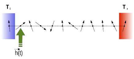
Figure 1: (Color online) Schematic diagram of the classical Heisenberg model in one dimension with two boundary heat baths at temperatures $T_{l}$ and $T_{r}$, and local time varying magnetic field $\vec{h}(t)$ that acts on the first site of the system $i=1$. We choose $T_{l}<T_{r}$ and $\vec{h}(t)\equiv(0,0,A\sin(\omega t))$.

Consider classical Heisenberg spins $\{\vec{S_{i}}\}$ (three-dimensional unit vectors) on a one-dimensional regular lattice of length $N$ $(1\leq i\leq N)$ and the Hamiltonian of the system is given as,

$$\mathcal{H}=-K\sum_{i=1}^{N}\vec{S}_{i}\cdot\vec{S}_{i+1}-\vec{h}(t)\cdot\vec{S}_{i}\delta_{i1},$$ (1)

where the spin-spin interaction is ferromagnetic for coupling $K>0$ and anti-ferromagnetic for $K<0$. The second term Eq. (1) is due to a time varying magnetic field that acts locally on the spin at the first site $i=1$. A schematic diagram of our system is shown in Fig. 1. The microscopic equation of motion for the spin vectors can be written as

$$\frac{d}{dt}{\vec{S}_{i}}=\vec{S}_{i}\times\left[\vec{B}_{i}+\vec{h}(t)\delta_{i1}\right],$$ (2)

where $\vec{B}_{i}=K(\vec{S}_{i-1}+\vec{S}_{i+1})$ is the local molecular field experienced by the spin at site $i$. Apart from the local forcing, there is also an overall thermal gradient across the system maintained by two heat baths attached at the two boundaries. This is implemented by introducing to additional spins at sites $i=0$ and $i=N+1$. The bonds between the pairs of spins ($\vec{S}_{0},\vec{S}_{1}$) and ($\vec{S}_{N},\vec{S}_{N+1}$) at two opposite ends of the system behave as stochastic thermal baths. The left and right baths are in equilibrium at their respective temperatures, $T_{l}$ and $T_{r}$ and the bond energies $E_{l}=-K\vec{S}_{0}\cdot\vec{S}_{1}$ and $E_{r}=-K\vec{S}_{N}\cdot\vec{S}_{N+1}$ have a Boltzmannian distribution. The interaction strength of the bath spins with the system is taken to be $K$, and therefore both $E_{l}$ and $E_{r}$ are bounded in the range $(-K,K)$. Thus the average energies of the baths are given by $\langle E_{l}\rangle=-K\mathcal{L}(K/T_{l})~{}{\rm and}~{}\langle E_{r}\rangle=-K\mathcal{L}(K/T_{r})$, $\mathcal{L}(x)$ being the standard Langevin function. Thus one can set the two baths at a fixed average energy (or temperature) and a thermal current flows through the system if $T_{l}\neq T_{r}$. For our simulations we choose $T_{l}<T_{r}$ and therefore the periodic forcing is near the colder boundary.

We investigate the steady state transport properties of the Heisenberg model by numerically computing quantities, such as, currents, energy profiles etc. using the DTOE dynamics our . Briefly stated, the DTOE dynamics updates the spins belonging to the odd and even sub-lattices alternately using a spin precessional dynamics

$$\vec{S}_{i,t+1}=\left[\vec{S}\cos\phi+(\vec{S}\times\hat{B})\sin\phi+(\vec{S}\cdotp\hat{B})\hat{B}(1-\cos\phi)\right]_{i,t},$$ (3)

where $\hat{B}_{i}=\vec{B}_{i}/|\vec{B}_{i}|$, $\phi_{i}=|\vec{B}_{i}|\Delta t$ and $\Delta t$ is the integration time step. The above formula is also sometimes referred to as the rotation formula and holds for rotation of any finite magnitude goldstein . Note that $\vec{B}_{i}$ in the above equation has to be replaced by the vector ($\vec{B}_{i}+\vec{h}(t))$ for the first site $i=1$. The advantages of using the DTOE dynamics are as follows. This dynamics is strictly energy conserving and maintains the length of the spin vectors naturally. The total spin conservation is also approximately maintained and is comparatively better than other conventional integration schemes sdiff . Also it has been thoroughly verified that local thermal equilibrium is established in the thermally driven system (in absence of forcing) when evolved using the DTOE dynamics independently of the value of the integration time step $\Delta t$. A thorough discussion of the DTOE scheme and numerical implementation of the thermal baths have been presented in Ref. our .

The computation of the steady state thermal current is done as described in the following. Since the DTOE dynamics alternately updates only half of the spins (odd/even) but all the bond energies simultaneously, the energy of the bonds $E^{o}_{i}$ measured immediately after the update of odd spins is different from $E^{e}_{i}$ measured after the update of even spins where $E_{i}=-K\vec{S}_{i}\cdot\vec{S}_{i+1}-\vec{h}(t)\cdot\vec{S}_{i}\delta_{i1}$. Clearly, the difference $E^{e}_{i}-E^{o}_{i}$ is a measure of the energy flowing through the $i$-th bond in time $\Delta t$. Thus the thermal current (rate of flow of thermal energy) in the steady state is given by

$$j=\langle E^{e}_{i}-E^{o}_{i}\rangle/\Delta t$$ (4)

and the average energy of $i$-th bond is $E_{i}=\frac{1}{2}\langle E^{e}_{i}+E^{o}_{i}\rangle$. As already mentioned, the thermal current $j$ in the one dimensional classical Heisenberg model obeys the Fourier law, i.e., $j\sim 1/N$. Let us define a total current $J\equiv jN$ which clearly is independent of the system size. In the following, we present our numerical results in terms of the total current $J$, since this will allow us to compare the thermal current of systems of different sizes.

III Numerical Results

III.1 Resonance

For simulations, we choose the time varying magnetic field of the form $\vec{h}(t)\equiv(0,0,A\sin(\omega t))$ and the boundary heat baths have average energy $\langle E_{l}\rangle=E_{b}$ and $\langle E_{r}\rangle=E_{b}+\Delta E$. Starting from a random initial configuration of spins, the system is evolved using the DTOE dynamics with integration time-step $\Delta t=0.25$. The spin system is first relaxed, typically for $\sim 10^{6}-10^{7}$ iterations, and thereafter the steady state quantities are computed for the next $\sim 10^{7}-10^{8}$ iterations which is also averaged over several independent realizations (typically $\sim 1000$) of the initial spin configuration. In absence of periodic forcing, a current flows through the system in response to the imposed thermal bias. To fix the sign of the thermal current we set the following convention - a current flowing from a larger to a smaller site index $i$ is negative; in other words, a current from the right towards the left end of the lattice is taken to be negative and vice-versa.

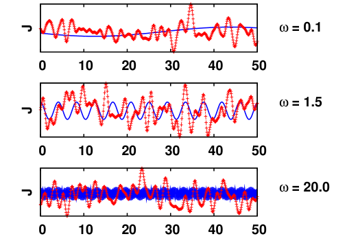
Figure 2: (Color online) Typical oscillations of the total thermal current $J$ (data points shown as ‘+’ symbol) in the steady state at small ($\omega=0.1$), moderate ($\omega=1.5$) and high ($\omega=20.0$) frequencies along with the corresponding time varying magnetic field (smooth continuous lines). Thermal resonance occurs in our model at frequency $\omega\approx 1.5$ where the typical oscillation frequency of the current becomes comparable to the periodic forcing frequency.

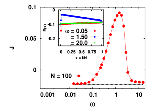
Figure 3: (Color online) Thermal resonance in classical Heisenberg model: (a) thermal current $J$ shows thermal resonance for some value of the forcing frequency $\omega\approx 1.5$ where the $J(\omega)$ curve shows a peak. The low and high frequency behavior is same as that in absence of any periodic forcing (shown as a dotted line); The parameters used are $N=100,A=1.0,E_{b}=-0.1$, and $\Delta E=0.015$. (Inset) The change of sign of the slope of the energy profile for $\omega=1.5$ as compared to $\omega=0.05,20.0$ suggests current reversal in the bulk of the system.

We categorize the frequency response of the system in three separate regimes - the low, moderate and high frequency. For comparison, we plot the thermal current $J$ and the periodic forcing as a function of time, for three frequencies corresponding to the three regimes mentioned above. This is shown in Fig. 2 where we have shown the thermal current and the sinusoidal forcing field for frequencies $\omega=0.1,1.5,20.0$. The steady state current as a function of the forcing frequency is shown in Fig. 3. We find that the thermal transport scenario is essentially the same for the small and high frequency regimes. For small values of the forcing frequency the current flows through the system from the higher temperature end to the lower temperature end (hence negative according to our convention) and similarly for high frequencies, and the average value of the current is roughly the same in these to regimes. This can be understood from the fact that for very small frequencies the typical timescales of the system are much smaller than the forcing timescale and thus the system senses two opposite static forces which amounts to no net forcing. In the other limit, the system fails to respond to the rapidly varying forcing and thus effectively experiences no external forcing. Thus in the two asymptotic limits the frequency behavior is essentially the same as can be clearly seen from Fig. 3.

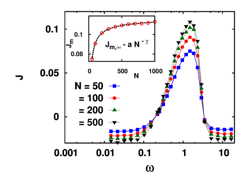
Figure 4: (Color online) Thermal resonance survives in the thermodynamic limit as can understood from the $J(\omega)$ curve for system sizes $N=50,100$ and $200$, all other parameters remaining the same as Fig. 3. (Inset) The maximum current $J_{m}$ corresponding to $\omega=\omega_{m}$ saturates in the thermodynamic limit. The $J_{m}\sim N$ data obtained from simulation fits with the form $J_{m,\infty}-aN^{-\gamma}$ (shown as a broken line) where $J_{m,\infty}=0.118$, $a=0.633$, and $\gamma=0.685$.

In the moderate frequency range, where the typical oscillations of the thermal current is comparable to that of the external periodic forcing, the current however shows thermal resonance - the current attains a maximum value $J_{m}$ corresponding to some characteristic resonance frequency $\omega_{m}$. By properly choosing the bath temperatures, the current $J$ can even be made to change sign (here, from negative to a positive value). This implies that for certain range of the forcing frequency the thermal current through the bulk of the system flows in the opposite direction i.e., from the colder end to the hotter end. We refer to this frequency range for which the bulk current is reversed as the resonance region for convenience sake.

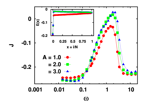
Figure 5: (Color online) (a) Thermal resonance with a larger energy gradient ($E_{b}=-0.2$ and $\Delta E=0.175$) for different values of the forcing amplitude $A$. Increasing the amplitude increases the current and makes $J>0$; (Inset) Energy profiles corresponding to $A=1.0,2.0$ and $3.0$ for $N=100$. The energy profile for $A=1.0$ has slope of opposite sign as compared to that for $A=2.0$ and $3.0$.

To check that the thermal current indeed gets reversed for frequencies in the resonance region, we compute the energy profile of the system [see Fig. 3 (inset)] for three forcing frequencies belonging to the three frequency regimes. It is found that the energy profiles for small and large frequencies have the usual linear form connecting the two heat baths with a discontinuity at the forcing site. The energy profile for frequency in the resonance region $\omega=1.5$, however, has an opposite slope in the bulk of the system. Thus by merely tuning the forcing frequency, one can easily manipulate the magnitude as well as the direction of flow of the thermal current in the bulk of the system. Two more characteristic features of the observed thermal resonance are in order. Firstly, the resonance effect survives in the thermodynamic limit which is evident from Fig. 4, where we have shown resonance for three different system sizes. The maximum current $J_{m}$ as a function of the system size fits nicely with the functional form $J_{m}=J_{m,\infty}-aN^{-\gamma}$, where $J_{m,\infty}$ is the saturation value of maximum current in the thermodynamic limit, and $a,\gamma$ are fitting parameters. Thus the maximum current has a finite limiting value for a thermodynamically large system. This evidently shows that thermal resonance is an intrinsic feature of the system and not a finite size effect. Secondly, the resonance frequency $\omega_{m}$ seems to be completely independent of the system size, which again points to the fact that the $\omega_{m}$ is an intrinsic frequency of the system.

If the temperature gradient is comparatively large (keeping all other parameters unchanged), the resonance phenomenon is still there but the current through the system has now a large negative value and tuning only the frequency can not push the current to a positive value. As before, the energy profiles can be computed which also validate the fact that the current although is amplified (the slope of the energy profile increases) but does not get reversed (the slope does not change sign). This is shown in Fig. 5. However, increasing the amplitude can push the current to a positive value and current reversal can be achieved in the bulk of the system.

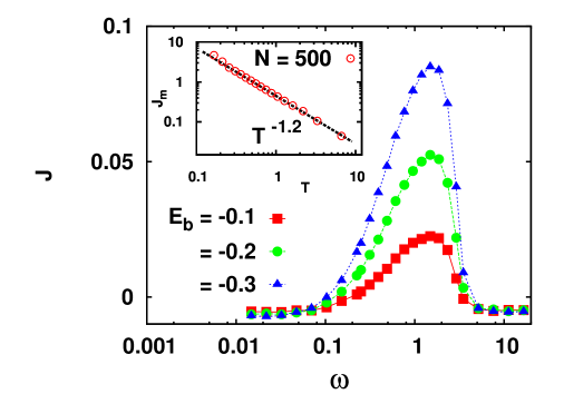
Figure 6: (Color online) Thermal current with frequency for different average energy of the bath $E_{b}=-0.1,-0.2$ and $-0.3$ and same energy gradient $\Delta E=0.015$. Resonance enhances as the temperature decreases. (Inset) Log-log plot of the maximum thermal current $J_{m}$ corresponding to $\omega=1.5$ for $N=500$.

We also investigate the effect of the temperature on the resonance feature. Let the temperatures of the two baths be $T_{l}=T$ and $T_{r}=T+\Delta T$. For the same $\Delta T$ we find that the resonance effect is enhanced at a lower temperature and the current amplification is larger as is shown in Fig. 6. To see how the maximum thermal current $J_{m}$ varies with temperature, we set $\omega=\omega_{m}\approx 1.5$ and measure $J_{m}$ for different bath temperatures keeping the same temperature difference. The inset in Fig. 6 suggests that the maximum current $J_{m}$ is inversely proportional (approximately) to the temperature of the system. Phenomenologically, the total thermal current in a finite system can be related to its size via the relation our

$$J=\kappa\frac{N\Delta E}{N+\xi},$$ (5)

where $\kappa$ is the thermal conductivity and $\xi$ is the correlation length of the system, both being a function of the temperature. Since both $\kappa$ and $\xi$ vary as $T^{-1}$ at low temperatures our , the above relation suggests that, in the thermodynamically large system ($N\gg\xi$), $J_{m}\sim T^{-1}$. Thus our numerical result is found to be close to this analytical result but needs corrections for finite size.

III.2 Multiresonance

For certain parameter ranges, the thermal resonance described above can show multiresonance behavior in which the resonance peak splits into two or more distinct resonance peaks. In the following, we study the multiresonance phenomenon and its dependence on the system parameters. In Fig. 7 the thermal current $J$ is shown as a function of the forcing frequency $\omega$ for several values of the forcing amplitude $A$. We find that as $A$ increases, first, the central peak splits up in two peaks and the current $J$ corresponding to $\omega=\omega_{m}$ is no longer the maximum now; two other peaks appear on both sides of $\omega_{m}$. Thus in Fig. 7 we find that for $A=5.0$ there are two peaks, whereas, for $A=7.0$ there are three peaks, and for $A=9.0$ four peaks appear which are further amplified as $A$ increases. This process continues and new peaks emerge as the forcing amplitude is increased. Thus multiresonance is enhanced as the amplitude of the forcing is increased.

We also find that the multiresonance feature gets magnified as the average temperature of the system goes down, similar to the previous case of single peak resonance. For the FK model, multiresonace is seen both in the limit of low and high temperatures since the model reduces to an effective harmonic model in both the limits, whereas, in the intermediate temperature range there occurs a crossover from single peak to multiresonace multi . In Fig. 8a we show the multiresonace in our model for different values of the average bath energy $E_{b}$. This enhancement in multiresonance can be explained by considering the fact that the classical Heisenberg model at low temperatures can be effectively thought to be a harmonic-like system our in terms of the relevant degrees of freedom (here, the angle between the spin vectors $\theta_{i}$). This is similar to the case of FK model, where with the increase (or decrease) of temperature a harmonic-like behavior emerges. Since resonant magnitudes are larger in the harmonic lattice as compared to the FK model multi , we expect an enhanced multiresonance in the Heisenberg model at lower temperatures. However, the number of resonance peaks seem to be independent of the average temperature of the system.

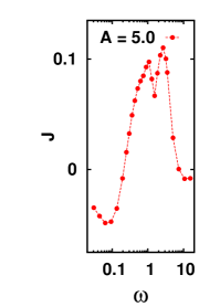
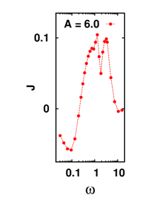
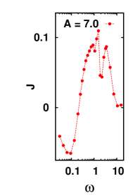
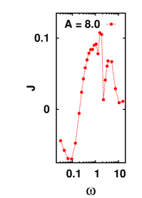
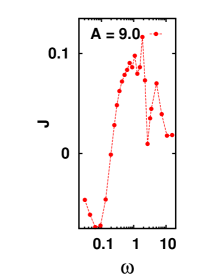
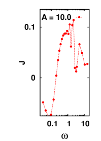
Figure 7: (Color online) The thermal current $J$ for forcing amplitude $A=5.0,6.0,7.0,8.0,9.0$ and $10.0$, for bath energy $E_{b}=-0.1$ with $\Delta E=0.015$ in a system size of $N=100$ shows more than one resonance peak as the forcing amplitude $A$ is increased.

The multiresonace feature of our model, however, appears to be different from that of the FK/harmonic lattices in the sense that only a few spin modes are excited as the forcing amplitude is increased. It is also observed (from the data shown in Fig. 7) that a modal frequency which is a dominant mode of energy transport for a given forcing amplitude does not always remain a dominant mode when the amplitude is altered. For example, the dominant frequency for $A=1.0$ which approximately corresponds to $\omega_{m}=1.5$ is no longer a dominant mode for $A=5.0$; two other frequencies on either side of $\omega_{m}$ become the dominant modal frequencies that contribute the most to the thermal transport. Unlike the harmonic system where the amplitude of the forcing signal excites all the eigenmodes of the system, here, external forcing selectively picks up certain frequencies and amplifies them. This disparity is also apparent from the fact that the number of modes that are excited by the external forcing seems to be independent of the system size as can be seen in Fig. 8b. For the harmonic system, the number of modes participating in transport is directly proportional to the size of the system which is definitely not the case in our model.

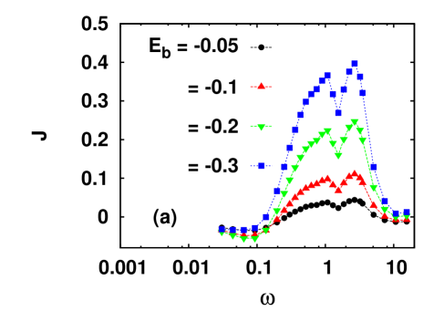
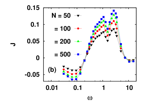
Figure 8: (Color online) (a) The thermal current $J$ for different average bath energy $E_{b}=-0.05,-0.1,-0.2$ and $-0.3$, with $\Delta E=0.015$ and forcing amplitude $A=5.0$ for a system size of $N=100$. (b) The thermal current $J$ for different system sizes $N=50,100,200$ and $500$ with $A=5.0$, $E_{b}=-0.1$ and with $\Delta E=0.015$.

We have also increased the data sampling frequency to resolve finer structures, if present, within the broad multiresonace peaks but could not find any, even for very small systems at low temperatures for which the harmonic approximation should be valid. Thus we speculate that, although nonlinearty effects are relatively suppressed at low temperatures (where our model has an effective harmonic description), they do not vanish completely and spin modes remain strongly coupled to each other. Unlike the FK model, increasing the forcing amplitude to quite larger values in this model can excite only a few spin modes because of the existence of strong intrinsic nonlinearity. A more detailed study of the classical Heisenberg model is surely desirable to unravel the underlying physics of its multiresonance feature.

III.3 Absence of thermal pumping

Although the system in resonance exhibits a reversed bulk current, there is no thermal pumping in this system. This is consistent with the result (previously obtained for FK/harmonic lattices) that there is no thermal pumping in force-driven lattices. For a system to be a thermal pump, energy must be pumped from the colder heat bath and absorbed in the hotter heat bath and as a consequence a reverse flow of energy occurs in the bulk of the system. However in our system (and other force-driven lattices in general), although the high temperature bath absorbs energy from the system and a reversed current flows through the bulk, the low temperature heat bath does not pump energy into the bulk of the system. What actually happens is that the additional energy, drawn from the external periodic forcing, flows from the point of forcing (here $i=1$) towards the two boundaries of the system, and thus, results in a reversed bulk current.

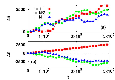
Figure 9: (Color online) Computation of $\Delta n=n_{l}-n_{r}$ from a typical run using the DTOE dynamics for three sites $i=1,N/2$ and $N$ in a system of size $N=100$, $E_{b}=-0.1$, $\Delta E=0.015$: (a) without periodic forcing energy across all the sites flow towards left; (b) with periodic forcing ($A=1.0$, $\omega=1.5$) energy across site $i=1$ flow towards left whereas, for sites $i=N/2$ and $N$ flows to the right. Thus both the heat baths absorb energy and there is no thermal pumping.

This can be clearly seen in our system by monitoring the energy flow across sites $i=1,N/2$ and $N$. When the spin at a site $i$ is updated using the DTOE dynamics, the energy of the bonds connected to it, namely $E_{i-1}$ and $E_{i}$, are updated such that the sum $E_{i-1}+E_{i}$ remains the same before and after the update. In other words, a redistribution of the sum $E_{i-1}+E_{i}$ takes place while the $i$-th spin is updated. Since our system is connected to stochastic thermal baths, this redistribution process is also stochastic in nature - the $(i-1)$-th bond stochastically gains and loses energy and similarly for the $i$-th bond. However, since there is an overall thermal gradient $(T_{r}-T_{l})$, the total number of times energy flows in one particular direction (here, towards left since $T_{r}>T_{l}$) over a long time will obviously be more than that of the opposite direction so that a steady energy current flows through the system. In absence of the periodic forcing, the quantity $\Delta n=n_{l}-n_{r}$ is positive when measured for sites $i=1,N/2$ and $N$, where $n_{l}$ ($n_{r}$) is the total number of times energy flows to the left (right) across a particular site. The results from a typical run, starting from a random initial condition of spins and using the DTOE dynamics, is shown in Fig. 9a. Thus energy flows from the high energy bath to the low energy bath i.e., from right to left end of the system. However when the system is in resonance region, $\Delta n$ for site $i=1$ is positive whereas that for sites $i=N/2$ and $N$ is negative. This shows that while in resonance, energy flows from right to left for $i=1$ but for $i=N/2$ and the right end $i=N$, energy flows from left to right (see Fig. 9b). Thus current flows towards the two boundaries from the point of periodic perturbation in the bulk of the system. Evidently, there is no thermal pumping since both the high temperature and low temperature baths absorb energy and thus the transport of energy from low to high temperature bath is absent.

IV Summary

To summarise, we report here the extensive numerical study of the one dimensional classical Heisenberg model in presence of boundary drive and time varying forcing. A time-periodic magnetic field acts locally at one end of the system (site $i=1$) and a thermal gradient is maintained by boundary heat baths. We choose the time-periodic forcing to be sinusoidal with amplitude $A$ and frequency $\omega$. The thermal current that flows though the system shows resonance at some characteristic frequency $\omega_{m}$ of the forcing frequency for which the current attains a maximum value. By properly tuning the boundary temperatures, we demonstrate that the energy current flowing through the bulk of the system can be reversed for frequencies within the resonance region. The magnitude of the current can also be controlled by tuning the forcing amplitude $A$. This allows one to mechanically control the magnitude as well as the direction of current in the system. This could be of immense practical use in nanoscale systems where a large thermal gradient is not desirable.

We study the dependence of the thermal resonance on the parameters of the system. It is found that the magnitude of resonance increases as the system size increases and survives in the thermodynamic limit. The maximum thermal current $J_{m}$ corresponding to the resonance frequency $\omega_{m}$, saturates to a finite value for a thermodynamically large system. Also decreasing the average temperature enhances the magnitude of resonance; the maximum thermal current $J_{m}$ varies as $T^{-1}$ at low temperatures in the thermodynamic limit.

In some parameter range, the single resonance peak splits into multiple peaks and a multiresonance phenomenon is observed. As the amplitude of the external forcing is increased, the number of peaks also increases. The resonance and the multiresonace phenomenon can in general be explained as follows. The external periodic forcing that is imposed on the system acts as an additional source of energy for the system. When the frequency of the forcing coincides with the natural frequencies of the system, the transfer of energy from the external perturbation to the system becomes maximum. However for our system, certain frequencies are selectively excited by the external forcing and the the number of modal frequencies that participate in thermal transport is determined by the forcing amplitude. Similar to single peak resonance, the magnitude of multiresonance is also enhanced with the decrease of average temperature of the system; the modal frequencies and their number, however, seem to be independent of the average temperature and also the size of the system.

Finally, we explicitly show using energy flow arguments that despite the reversal of the current in the bulk, this system fails to act as a thermal pump. This is consistent with the previous result that a force-driven lattice can not direct thermal energy from the low temperature heat bath to the high temperature heat bath.

The classical model can be thought to be the infinitely large spin limit of the quantum Heisenberg model. This classical approximation of the quantum model is already seen to hold for systems with spin $s=5/2$, for example, in $Mn^{2+}$ windsor . As such, controlled laboratory experiments with model chemical compounds, which are now-a-days routinely performed, can be used to test the theoretical predictions made in the classical Heisenberg model. Hopefully, such experimental studies will eventually lead us towards better heat control and management in future.

Acknowledgement: The author would like to thank P. K. Mohanty for helpful suggestions and careful reading of the manuscript.

References

- (1) F. Bonetto, J. L. Lebowitz, and L. Rey-Bellet, Fourier law: A challenge to theorists, in Mathematical Physics 2.
- (2) S. Lepri, R. Livi, and A. Politi, Phys. Rep. 377, 1 (2003).
- (3) A. Dhar, Advances in Physics, 57, 457, (2008).
- (4) N. Li, J. Ren, L. Wang, G. Zhang, P. Hänggi, B. Li, Rev. Mod. Phys. 84, 1045-1066 (2012).
- (5) M. Terraneo, M. Peyrard, and G. Casati, Phys. Rev. Lett. 88, 094302 (2002); B. Li, L. Wang, and G. Casati, ibid. 93, 184301 (2004).
- (6) B. Li, L. Wang, and G. Casati, Appl. Phys. Lett. 88, 143501 (2006).
- (7) L. Wang and B. Li, Phys. Rev. Lett. 99, 177208 (2007).
- (8) L. Wang and B. Li, Phys. Rev. Lett. 101, 267203 (2008).
- (9) C. W. Chang, D. Okawa, H. Garcia, A. Majumdar, and A. Zettl, Phys. Rev. Lett. 99, 045901 (2007).
- (10) G. Casati, Chaos 15, 015120 (2005).
- (11) B. Hu and L. Yang, Chaos 15, 015119 (2005).
- (12) B. Ai, D. He, and B. Hu, Phys. Rev. E 81, 031124 (2010).
- (13) S. Zhang, J. Ren, and B. Li, Phys. Rev. E 84, 031122 (2011).
- (14) F. Geniet and J. Leon, Phys. Rev. Lett. 89, 134102 (2002).
- (15) R. Khomeriki, S. Lepri, and S. Ruffo, Phys. Rev. E 70, 066626 (2004).
- (16) P. Maniadis, G. Kopidakis, and S. Aubry, Physica D 216, 121 (2006).
- (17) T. Dauxois, R. Khomeriki, and S. Ruffo, Eur. Phys. J. Spec. Top. 147, 3 (2007).
- (18) M. Johansson, G. Kopidakis, S. Lepri, and S. Aubry, Europhys. Lett. 86, 10009 (2009).
- (19) M. E. Fisher, Am. J. Phys. 32, 343 (1964).
- (20) G. S. Joyce, Phys. Rev. 155, 478 (1967).
- (21) F. Heidrich-Meisner, A. Honecker and W. Brenig, Eur. Phys. J. Special Topics 151, 135-145 (2007).
- (22) C. Hess, Eur. Phys. J. Special Topics 151, 73 (2007).
- (23) A. V. Sologubenko, T. Lorenz, H. R. Ott, and A. Freimuth, J. Low Temp. Phys. 147, 387 (2007).
- (24) A. V. Savin, G. P. Tsironis, and X. Zotos, Phys. Rev. B 72, 140402(R) (2005).
- (25) D. Bagchi and P. K. Mohanty, Phys. Rev. B 86, 214302 (2012).
- (26) V. Oganesyan, A. Pal and D. Huse, Phys. Rv. B 80, 115104 (2009).
- (27) A. V. Savin, G. P. Tsironis, and X. Zotos, Phys. Rev. B 75, 214305 (2007).
- (28) V.V. Kruglyak, S.O. Demokritov, D. Grundler, J. Phys. D: Appl. Phys. 43 264001(2010).
- (29) B. Lenk, H. Ulrichs, F. Garbs, M. Münzenberg, Phys. Rep. 507, 107 (2011).
- (30) M. V. Costache, G. Bridoux, I. Neumann and S. O. Valenzuela, Nature Materials 11, 199 (2012).
- (31) H. Adachi, K. Uchida, E. Saitoh and S. Maekawa, Rep. Prog. Phys. 76, 036501 (2013).
- (32) H. Goldstein, C. P. Poole and J. L. Safko, Classical Mechanics, 3rd Edition, Addison Wesley.
- (33) D. Bagchi, Phys. Rev. B 87, 075133 (2013).
- (34) M. Steiner, J. Villain, and C. Windsor, Adv. Phys. 25, 87 (1976).