Non-dissipative space-time hp𝑝hp-discontinuous Galerkin method for the time-dependent Maxwell equations

M. Lilienthal lilienthal@gsc.tu-darmstadt.de S.M. Schnepp sascha.schnepp@ifh.ee.ethz.ch T. Weiland thomas.weiland@temf.tu-darmstadt.de Graduate School of Computational Engineering, Technische Universitaet Darmstadt, Dolivostrasse 15, 64293 Darmstadt, Germany ETH Zurich, Institute of Electromagnetic Fields (IFH), Gloriastrasse 35, 8092 Zurich, Switzerland Institut fuer Theorie Elektromagnetischer Felder, Technische Universitaet Darmstadt, Schlossgartenstrasse 8, 64289 Darmstadt, Germany
Abstract

A finite element method for the solution of the time-dependent Maxwell equations in mixed form is presented. The method allows for local hp𝑝hp-refinement in space and in time. To this end, a space-time Galerkin approach is employed. In contrast to the space-time DG method introduced in [1] test and trial space do not coincide. This allows for obtaining a non-dissipative method. To obtain an efficient implementation, a hierarchical tensor product basis in space and time is proposed. This allows to evaluate the local residual with a complexity of 𝒪(p4)𝒪superscript𝑝4\mathcal{O}(p^{4}) and 𝒪(p5)𝒪superscript𝑝5\mathcal{O}(p^{5}) for affine and non-affine elements, respectively.

1 Introduction

The accurate solution of large scale electromagnetic problems, where short wavelengths need to be resolved in large computational domains, remains a challenge. Examples include antenna design, broadband scattering problems or electrically large structures. Especially for problems, where dispersion errors dominate, high order methods have advantages. Furthermore, if hp𝑝hp-refinement is applied in a judicious way, it is possible to obtain exponential convergence, even for solutions, which are locally non-smooth [2]. This can lead to drastical savings in terms of degrees of freedom. In the past decade, there has been a lot of research on discontinuous Galerkin (DG) methods for Maxwell’s equations, see e.g. [3, 4, 5]. The use of discontinuous finite element spaces, allows in a natural way for hp𝑝hp-refinement without the use of special transition elements as it is the case for continuous finite element methods [6, 7]. Often, DG methods are chosen for the spatial part of the discretization, whereas time is discretized with explicit time integrators. Due to the conditional stability of the resulting schemes, the time step size in this case is determined by the smallest element and also the degree of the approximating polynomials. Thus, the temporal resolution is dictated by stability, not by actual accuracy requirements. To overcome this problem, local time-stepping schemes [5, 8, 9] and locally implicit schemes [10, 11] have been proposed. For both approaches, good speedups on locally refined meshes are reported. However, refinement in time is necessary for stability, rather than accuracy requirements.
Another approach are space-time DG methods [1]. Since space and time are discretized simultaneously, hp𝑝hp-refinement in space and time can be introduced naturally. The space-time DG methods are unconditionally stable. Together with their high flexibility, these methods are well-suited for space-time adaptivity. However, many of the previously introduced space-time DG methods are dissipative. Dissipation may become an issue, especially for low approximation orders. In this paper we propose a space-time finite element method which is discontinuous with respect to the spatial directions and continuous in time. For a similar approach, regarding the temporal part of the discretization, see the recent contribution [12], where a hh-version hybrid DG method in space, combined with a global continuous Galerkin approach in time is presented for the accoustic wave equation. However, we obtain a method, which allows for local hp𝑝hp-refinement in space and time, is energy-conserving and unconditionally stable. In section 2 the space-time finite element method for the time-dependent Maxwell equations

ε𝐄t×𝐇=𝐉inΩ×(0,T]𝜀subscript𝐄𝑡𝐇𝐉inΩ0𝑇\displaystyle\varepsilon\mathbf{E}_{t}-\nabla\times\mathbf{H}=\mathbf{J}\;\;\mbox{in}\;\Omega\times(0,T]
μ𝐇t+×𝐄=0inΩ×(0,T]𝜇subscript𝐇𝑡𝐄0inΩ0𝑇\displaystyle\mu\mathbf{H}_{t}+\nabla\times\mathbf{E}=0\;\;\mbox{in}\;\Omega\times(0,T]
𝐧×𝐄=𝐧×𝐠onΩ×(0,T]𝐧𝐄𝐧𝐠onΩ0𝑇\displaystyle\mathbf{n}\times\mathbf{E}=\mathbf{n}\times\mathbf{g}\;\;\mbox{on}\;\partial\Omega\times(0,T]
𝐄=𝐄0,𝐇=𝐇0inΩ,t=0formulae-sequence𝐄subscript𝐄0formulae-sequence𝐇subscript𝐇0inΩ𝑡0\displaystyle\mathbf{E}=\mathbf{E}_{0},\;\;\mathbf{H}=\mathbf{H}_{0}\;\mbox{in}\;\Omega,\;t=0 (1)

is described, where ε(𝐱),μ(𝐱):Ω:𝜀𝐱𝜇𝐱Ω\varepsilon(\mathbf{x}),\mu(\mathbf{x}):\Omega\rightarrow\mathbb{R} denote the electric permittivity and magnetic permeability, respectively. In sections 3 and 4 we discuss the stability and energy conservation property of the method. In section 5 we present a matrix-free implementation of the space-time residual. It can be efficiently evaluated within an interative solution procedure, such that the method computationally behaves similarly to an explicit method. Section 6 is devoted to numerical experiments, including fully space-time hp𝑝hp-adaptive simulations.

2 Description of the method

2.1 Function spaces

We will denote vector valued functions spaces with bold letters, e.g. 𝐋2(D):=[L2(D)]3assignsubscript𝐋2𝐷superscriptdelimited-[]subscript𝐿2𝐷3\mathbf{L}_{2}(D):=[L_{2}(D)]^{3}. We introduce the spaces

𝐇(curl,Ω):={𝐯𝐋2(Ω):×𝐯𝐋2(Ω)},assign𝐇𝑐𝑢𝑟𝑙Ωconditional-set𝐯subscript𝐋2Ω𝐯subscript𝐋2Ω\displaystyle\mathbf{H}(curl,\Omega):=\{\mathbf{v}\in\mathbf{L}_{2}(\Omega):\nabla\times\mathbf{v}\in\mathbf{L}_{2}(\Omega)\},
𝐇0(curl,Ω):={𝐯𝐋2(Ω):×𝐯𝐋2(Ω),𝐧×𝐯=0onΩ}.assignsubscript𝐇0𝑐𝑢𝑟𝑙Ωconditional-set𝐯subscript𝐋2Ωformulae-sequence𝐯subscript𝐋2Ω𝐧𝐯0onΩ\displaystyle\mathbf{H}_{0}(curl,\Omega):=\{\mathbf{v}\in\mathbf{L}_{2}(\Omega):\nabla\times\mathbf{v}\in\mathbf{L}_{2}(\Omega),\mathbf{n}\times\mathbf{v}=0\;\mbox{on}\,\partial\Omega\}.

For 𝐉=0,𝐠=0formulae-sequence𝐉0𝐠0\mathbf{J}=0,\mathbf{g}=0 the Maxwell system admits a unique solution 𝐔={𝐄,𝐇}𝐔𝐄𝐇\mathbf{U}=\{\mathbf{E},\mathbf{H}\} in (see e.g. [13]):

𝐕:=C0([0,T],𝐇0(curl,Ω))C1([0,T],𝐋2(Ω))×C0([0,T],𝐇(curl,Ω))C1([0,T],𝐋2(Ω)).assign𝐕superscript𝐶00𝑇subscript𝐇0𝑐𝑢𝑟𝑙Ωsuperscript𝐶10𝑇subscript𝐋2Ωsuperscript𝐶00𝑇𝐇𝑐𝑢𝑟𝑙Ωsuperscript𝐶10𝑇subscript𝐋2Ω\displaystyle\mathbf{V}:=C^{0}([0,T],\mathbf{H}_{0}(curl,\Omega))\cap C^{1}([0,T],\mathbf{L}_{2}(\Omega))\times C^{0}([0,T],\mathbf{H}(curl,\Omega))\cap C^{1}([0,T],\mathbf{L}_{2}(\Omega)).

2.2 Partitioning of the space-time domain

For the derivation of the method, we only consider spatial meshes consisting of hexahedra. Nevertheless, most of the presented work is applicable to tetrahedral meshes, as well.

We divide the time axis in intervals n=(tn1,tn]subscript𝑛subscript𝑡𝑛1subscript𝑡𝑛\mathcal{I}_{n}=(t_{n-1},t_{n}], and thus obtain a partitioning of the space-time cylinder ×ΩΩ\mathcal{I}\times\Omega in time slabs n×Ωsubscript𝑛Ω\mathcal{I}_{n}\times\Omega. For each time slab, the spatial domain ΩΩ\Omega is partitioned into non-overlapping (hexahedral) elements K𝐾K resulting in a triangulation 𝒯n(Ω)subscript𝒯𝑛Ω\mathcal{T}_{n}(\Omega). We require that 𝒯n(Ω)subscript𝒯𝑛Ω\mathcal{T}_{n}(\Omega) can be obtained by refinement of a coarse triangulation 𝒯¯(Ω)¯𝒯Ω\overline{\mathcal{T}}(\Omega). The obtained macro-elements are further bisected in temporal direction n×K=k=1NKIkK×Ksubscript𝑛𝐾superscriptsubscript𝑘1subscript𝑁𝐾superscriptsubscript𝐼𝑘𝐾𝐾\mathcal{I}_{n}\times K=\bigcup_{k=1}^{N_{K}}I_{k}^{K}\times K, such that we obtain a partition of the time slab n×Ωsubscript𝑛Ω\mathcal{I}_{n}\times\Omega in space-time elements IkK×K𝒮n(n×Ω)superscriptsubscript𝐼𝑘𝐾𝐾subscript𝒮𝑛subscript𝑛ΩI_{k}^{K}\times K\in\mathcal{S}_{n}(\mathcal{I}_{n}\times\Omega). Here 𝒮n(n×Ω)subscript𝒮𝑛subscript𝑛Ω\mathcal{S}_{n}(\mathcal{I}_{n}\times\Omega) denotes the resulting triangulation of the time slab.

\psaxes[labels=none,ticks=none]-¿(-0.7,-0.5)(-0.7,-0.5)(8.5,4.5) tnsubscript𝑡𝑛t_{n}tn+1subscript𝑡𝑛1t_{n+1}K1subscript𝐾1K_{1}K2subscript𝐾2K_{2}K3subscript𝐾3K_{3}K4subscript𝐾4K_{4}I14×K4superscriptsubscript𝐼14subscript𝐾4I_{1}^{4}\times K_{4}I24×K4superscriptsubscript𝐼24subscript𝐾4I_{2}^{4}\times K_{4}I13×K3superscriptsubscript𝐼13subscript𝐾3I_{1}^{3}\times K_{3}I23×K3superscriptsubscript𝐼23subscript𝐾3I_{2}^{3}\times K_{3}I33×K3superscriptsubscript𝐼33subscript𝐾3I_{3}^{3}\times K_{3}I43×K3superscriptsubscript𝐼43subscript𝐾3I_{4}^{3}\times K_{3}I12×K2superscriptsubscript𝐼12subscript𝐾2I_{1}^{2}\times K_{2}I22×K2superscriptsubscript𝐼22subscript𝐾2I_{2}^{2}\times K_{2}I11×K1superscriptsubscript𝐼11subscript𝐾1I_{1}^{1}\times K_{1}
Figure 1: Space-time partitioning of a time-slab

2.3 Discrete spaces

Let FKsubscript𝐹𝐾F_{K} denote the mapping from the unit cube K^=[0,1]3^𝐾superscript013\hat{K}=[0,1]^{3} with axes x^,y^,z^^𝑥^𝑦^𝑧\hat{x},\hat{y},\hat{z} to the physical element K=FK(K^)𝐾subscript𝐹𝐾^𝐾K=F_{K}(\hat{K}). Furthermore by DFK𝐷subscript𝐹𝐾DF_{K} we denote the jacobian matrix of FKsubscript𝐹𝐾F_{K}. The electric and magnetic fields are transformed with the covariant transformation 𝐯(x,t)=DFKT𝐯^(x^,t)oFK1𝐯𝑥𝑡𝐷superscriptsubscript𝐹𝐾𝑇^𝐯^𝑥𝑡𝑜superscriptsubscript𝐹𝐾1\mathbf{v}(x,t)=DF_{K}^{-T}\hat{\mathbf{v}}(\hat{x},t)oF_{K}^{-1}, as proposed in [5].
By Ppt(I)subscript𝑃subscript𝑝𝑡𝐼P_{p_{t}}(I) we denote polynomials of degree ptsubscript𝑝𝑡p_{t} on interval I𝐼I and by Qpx,py,pz(K^)subscript𝑄subscript𝑝𝑥subscript𝑝𝑦subscript𝑝𝑧^𝐾Q_{p_{x},p_{y},p_{z}}(\hat{K}) tensor product polynomials of degrees px,pysubscript𝑝𝑥subscript𝑝𝑦p_{x},p_{y} and pzsubscript𝑝𝑧p_{z} in the x^,y^,z^^𝑥^𝑦^𝑧\hat{x},\hat{y},\hat{z} directions.
Now we can introduce the following local discrete spaces

Vh,K^k:=Ppt(IkK)[Qpx,py,pz(K^)]3assignsubscriptsuperscript𝑉𝑘^𝐾tensor-productsubscript𝑃subscript𝑝𝑡superscriptsubscript𝐼𝑘𝐾superscriptdelimited-[]subscript𝑄subscript𝑝𝑥subscript𝑝𝑦subscript𝑝𝑧^𝐾3\displaystyle V^{k}_{h,\hat{K}}:=P_{p_{t}}(I_{k}^{K})\otimes\left[Q_{p_{x},p_{y},p_{z}}(\hat{K})\right]^{3} (2)
Wh,K^k:=Ppt1(IkK)[Qpx,py,pz(K^)]3.assignsubscriptsuperscript𝑊𝑘^𝐾tensor-productsubscript𝑃subscript𝑝𝑡1superscriptsubscript𝐼𝑘𝐾superscriptdelimited-[]subscript𝑄subscript𝑝𝑥subscript𝑝𝑦subscript𝑝𝑧^𝐾3\displaystyle W^{k}_{h,\hat{K}}:=P_{p_{t}-1}(I_{k}^{K})\otimes\left[Q_{p_{x},p_{y},p_{z}}(\hat{K})\right]^{3}. (3)

𝐩kK=(pt,px,py,pz)superscriptsubscript𝐩𝑘𝐾subscript𝑝𝑡subscript𝑝𝑥subscript𝑝𝑦subscript𝑝𝑧\mathbf{p}_{k}^{K}=(p_{t},p_{x},p_{y},p_{z}) denotes the local polynomial degree vector assigned to the space-time elements IkK×K^,k=1,NKformulae-sequencesuperscriptsubscript𝐼𝑘𝐾^𝐾𝑘1subscript𝑁𝐾I_{k}^{K}\times\hat{K},k=1,\ldots N_{K}. Note that the spatial part of the polynomial spaces in (2) is identical for all elements IkK×K^superscriptsubscript𝐼𝑘𝐾^𝐾I_{k}^{K}\times\hat{K} in one macro-element n×K^subscript𝑛^𝐾\mathcal{I}_{n}\times\hat{K}. Thus we obtain, for each macro-element, tensor-product polynomial test- and trial-spaces consisting of a piecewise polynomial temporal trial- and test spaces SK(n)subscript𝑆𝐾subscript𝑛S_{K}(\mathcal{I}_{n}) and TK(n)subscript𝑇𝐾subscript𝑛T_{K}(\mathcal{I}_{n}) and the spatial part Qpx,py,pz(K^)subscript𝑄subscript𝑝𝑥subscript𝑝𝑦subscript𝑝𝑧^𝐾Q_{p_{x},p_{y},p_{z}}(\hat{K}).

Vh,K^:=SK(n)[Qpx,py,pz(K^)]3,SK(n):={u(t)H1(n):u|IkKPpt(IkK)}formulae-sequenceassignsubscript𝑉^𝐾tensor-productsubscript𝑆𝐾subscript𝑛superscriptdelimited-[]subscript𝑄subscript𝑝𝑥subscript𝑝𝑦subscript𝑝𝑧^𝐾3assignsubscript𝑆𝐾subscript𝑛conditional-set𝑢𝑡superscript𝐻1subscript𝑛evaluated-at𝑢superscriptsubscript𝐼𝑘𝐾subscript𝑃subscript𝑝𝑡superscriptsubscript𝐼𝑘𝐾\displaystyle V_{h,\hat{K}}:=S_{K}(\mathcal{I}_{n})\otimes\left[Q_{p_{x},p_{y},p_{z}}(\hat{K})\right]^{3},\;\;\;S_{K}(\mathcal{I}_{n}):=\{u(t)\in H^{1}(\mathcal{I}_{n}):{\left.\kern-1.2ptu\vphantom{\big{|}}\right|_{I_{k}^{K}}}\in P_{p_{t}}(I_{k}^{K})\}
Wh,K^:=TK(n)[Qpx,py,pz(K^)]3,TK(n):={u(t)L2(n):u|IkKPpt1(IkK)}.formulae-sequenceassignsubscript𝑊^𝐾tensor-productsubscript𝑇𝐾subscript𝑛superscriptdelimited-[]subscript𝑄subscript𝑝𝑥subscript𝑝𝑦subscript𝑝𝑧^𝐾3assignsubscript𝑇𝐾subscript𝑛conditional-set𝑢𝑡subscript𝐿2subscript𝑛evaluated-at𝑢superscriptsubscript𝐼𝑘𝐾subscript𝑃subscript𝑝𝑡1superscriptsubscript𝐼𝑘𝐾\displaystyle W_{h,\hat{K}}:=T_{K}(\mathcal{I}_{n})\otimes\left[Q_{p_{x},p_{y},p_{z}}(\hat{K})\right]^{3},\;\;\;T_{K}(\mathcal{I}_{n}):=\{u(t)\in L_{2}(\mathcal{I}_{n}):{\left.\kern-1.2ptu\vphantom{\big{|}}\right|_{I_{k}^{K}}}\in P_{p_{t}-1}(I_{k}^{K})\}. (4)

We collect the local polynomial degree vectors for all elements in a global vector 𝐩𝐩\mathbf{p}.
Now we can define the global spaces for one time-slab

Vh(n×Ω;𝐩):={𝐯(t,𝐱)H1(n;L2(Ω)):DFT𝐯|KoFVh,K^},assignsubscript𝑉subscript𝑛Ω𝐩conditional-set𝐯𝑡𝐱superscript𝐻1subscript𝑛subscript𝐿2Ωevaluated-at𝐷superscript𝐹𝑇𝐯𝐾𝑜𝐹subscript𝑉^𝐾V_{h}(\mathcal{I}_{n}\times\Omega;\mathbf{p}):=\{\mathbf{v}(t,\mathbf{x})\in H^{1}(\mathcal{I}_{n};L_{2}(\Omega)):DF^{T}{\left.\kern-1.2pt\mathbf{v}\vphantom{\big{|}}\right|_{K}}oF\in V_{h,\hat{K}}\}, (5)

and

Wh(n×Ω;𝐩):={𝐯(t,𝐱)L2(n;L2(Ω)):DFT𝐯|KoFWh,K^}.assignsubscript𝑊subscript𝑛Ω𝐩conditional-set𝐯𝑡𝐱subscript𝐿2subscript𝑛subscript𝐿2Ωevaluated-at𝐷superscript𝐹𝑇𝐯𝐾𝑜𝐹subscript𝑊^𝐾W_{h}(\mathcal{I}_{n}\times\Omega;\mathbf{p}):=\{\mathbf{v}(t,\mathbf{x})\in L_{2}(\mathcal{I}_{n};L_{2}(\Omega)):DF^{T}{\left.\kern-1.2pt\mathbf{v}\vphantom{\big{|}}\right|_{K}}oF\in W_{h,\hat{K}}\}. (6)

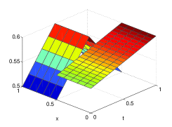
While both spaces are spatially discontinuous, the functions in Vhsubscript𝑉V_{h} and Whsubscript𝑊W_{h} have different continuity properties in temporal direction: functions in Vhsubscript𝑉V_{h} are time-continuous within each time slab whereas functions in Whsubscript𝑊W_{h} are allowed to be discontinuous at the interfaces in time direction. The situation is depicted for an example with three space-time elements in Fig. 2.
Refer to caption Refer to caption
Figure 2: Left: function belonging to trial space Vhsubscript𝑉V_{h}, right: function from the corresponding test space Whsubscript𝑊W_{h}

2.4 Faces and trace operators

By \mathcal{F} we denote the set of all faces in the spatial triangulation 𝒯(Ω)𝒯Ω\mathcal{T}(\Omega), by 0subscript0\mathcal{F}_{0} the set of all interior faces f:=K1K2:K1,K2𝒯(Ω):assign𝑓superscript𝐾1superscript𝐾2superscript𝐾1superscript𝐾2𝒯Ωf:=\partial K^{1}\cap\partial K^{2}\;:\;K^{1},\;K^{2}\in\mathcal{T}(\Omega) and by bsubscript𝑏\mathcal{F}_{b} the set of all boundary faces f:=KΩ:K𝒯(Ω):assign𝑓𝐾Ω𝐾𝒯Ωf:=\partial K\cap\partial\Omega\;:\;K\in\mathcal{T}(\Omega).
We define on interior faces f0𝑓subscript0f\in\mathcal{F}_{0} the average and tangential jump operators as {𝐯}:=(𝐯1+𝐯2)/2assign𝐯superscript𝐯1superscript𝐯22\{\mathbf{v}\}:=(\mathbf{v}^{1}+\mathbf{v}^{2})/2 and 𝐯T:=𝐧1×𝐯1+𝐧2×𝐯2\llbracket\mathbf{v}\rrbracket_{T}:=\mathbf{n}^{1}\times\mathbf{v}^{1}+\mathbf{n}^{2}\times\mathbf{v}^{2} respectively. Here 𝐯1superscript𝐯1\mathbf{v}^{1} and 𝐯2superscript𝐯2\mathbf{v}^{2} denote the traces of 𝐯𝐯\mathbf{v} on f𝑓f taken from within element K1superscript𝐾1K^{1} and K2superscript𝐾2K^{2} with unit normals 𝐧1superscript𝐧1\mathbf{n}^{1} and 𝐧2superscript𝐧2\mathbf{n}^{2}. For a boundary face fb𝑓subscript𝑏f\in\mathcal{F}_{b} we define averages and jumps as {𝐯}:=𝐯assign𝐯𝐯\{\mathbf{v}\}:=\mathbf{v} and 𝐯T:=𝐧×𝐯\llbracket\mathbf{v}\rrbracket_{T}:=\mathbf{n}\times\mathbf{v}.

In the following section we consider the discretization of a single time-slab n×Ωsubscript𝑛Ω\mathcal{I}_{n}\times\Omega.

2.5 Weak formulation

Multiplying (1) by smooth test functions 𝐯,𝐰𝐯𝐰\mathbf{v},\mathbf{w}, integrating over a macro-element n×Ksubscript𝑛𝐾\mathcal{I}_{n}\times K and performing integration by parts of the terms involving the curl operator with respect to the spatial variables yields:

nKεt𝐄𝐯dxdtnK𝐇×𝐯dxdtsubscriptsubscript𝑛subscript𝐾𝜀subscript𝑡𝐄𝐯d𝑥d𝑡subscriptsubscript𝑛subscript𝐾𝐇𝐯differential-d𝑥differential-d𝑡\displaystyle\int_{\mathcal{I}_{n}}\int_{K}\varepsilon\partial_{t}\mathbf{E}\cdot\mathbf{v}\,\mathrm{d}x\,\mathrm{d}t-\int_{\mathcal{I}_{n}}\int_{K}\mathbf{H}\cdot\nabla\times\mathbf{v}\,\mathrm{d}x\,\mathrm{d}t
nK𝐧×𝐇𝐯dSdt=nK𝐉𝐯dxdtsubscriptsubscript𝑛subscript𝐾𝐧superscript𝐇𝐯differential-d𝑆differential-d𝑡subscriptsubscript𝑛subscript𝐾𝐉𝐯differential-d𝑥differential-d𝑡\displaystyle-\int_{\mathcal{I}_{n}}\int_{\partial K}\mathbf{n}\times\mathbf{H}^{*}\cdot\mathbf{v}\,\mathrm{d}S\,\mathrm{d}t=\int_{\mathcal{I}_{n}}\int_{K}\mathbf{J}\cdot\mathbf{v}\,\mathrm{d}x\,\mathrm{d}t
nKμt𝐇𝐰dxdt+nK×𝐄𝐰dxdtsubscriptsubscript𝑛subscript𝐾𝜇subscript𝑡𝐇𝐰d𝑥d𝑡subscriptsubscript𝑛subscript𝐾𝐄𝐰differential-d𝑥differential-d𝑡\displaystyle\int_{\mathcal{I}_{n}}\int_{K}\mu\partial_{t}\mathbf{H}\cdot\mathbf{w}\,\mathrm{d}x\,\mathrm{d}t+\int_{\mathcal{I}_{n}}\int_{K}\nabla\times\mathbf{E}\cdot\mathbf{w}\,\mathrm{d}x\,\mathrm{d}t
+nK𝐧×(𝐄𝐄)𝐰dSdt=0.subscriptsubscript𝑛subscript𝐾𝐧superscript𝐄𝐄𝐰differential-d𝑆differential-d𝑡0\displaystyle+\int_{\mathcal{I}_{n}}\int_{\partial K}\mathbf{n}\times(\mathbf{E}^{*}-\mathbf{E})\cdot\mathbf{w}\,\mathrm{d}S\,\mathrm{d}t=0. (7)

Then by replacing 𝐔h:={𝐄,𝐇}𝐕assignsubscript𝐔𝐄𝐇𝐕\mathbf{U}_{h}:=\{\mathbf{E},\mathbf{H}\}\in\mathbf{V} by the discrete fields 𝐄h,𝐇hVhsubscript𝐄subscript𝐇subscript𝑉\mathbf{E}_{h},\mathbf{H}_{h}\in V_{h}, summing over all n×Ksubscript𝑛𝐾\mathcal{I}_{n}\times K and choosing centered fluxes

𝐧×𝐄=𝐧×{𝐄h}f0,𝐧×𝐄=𝐧×𝐠fD,𝐧×𝐇=𝐧×{𝐇h},fformulae-sequence𝐧superscript𝐄𝐧subscript𝐄𝑓subscript0𝐧superscript𝐄𝐧𝐠𝑓subscript𝐷formulae-sequence𝐧superscript𝐇𝐧subscript𝐇𝑓\displaystyle\mathbf{n}\times\mathbf{E}^{*}=\mathbf{n}\times\{\mathbf{E}_{h}\}\;f\in\mathcal{F}_{0},\hskip 5.69046pt\mathbf{n}\times\mathbf{E}^{*}=\mathbf{n}\times\mathbf{g}\;f\in\mathcal{F}_{D},\hskip 5.69046pt\mathbf{n}\times\mathbf{H}^{*}=\mathbf{n}\times\{\mathbf{H}_{h}\},\;f\in\mathcal{F}

one obtains

Ch(𝐔𝐡,𝐕)=L(𝐕)subscript𝐶subscript𝐔𝐡𝐕𝐿𝐕\displaystyle C_{h}(\mathbf{U_{h}},\mathbf{V})=L(\mathbf{V})
Ch(𝐔𝐡,𝐕):=nΩεt𝐄h𝐯dxdt+nΩμt𝐇h𝐰dxdt+assignsubscript𝐶subscript𝐔𝐡𝐕subscriptsubscript𝑛subscriptΩ𝜀subscript𝑡subscript𝐄𝐯d𝑥d𝑡limit-fromsubscriptsubscript𝑛subscriptΩ𝜇subscript𝑡subscript𝐇𝐰d𝑥d𝑡\displaystyle C_{h}(\mathbf{U_{h}},\mathbf{V}):=\int_{\mathcal{I}_{n}}\int_{\Omega}\varepsilon\partial_{t}\mathbf{E}_{h}\cdot\mathbf{v}\,\mathrm{d}x\,\mathrm{d}t+\int_{\mathcal{I}_{n}}\int_{\Omega}\mu\partial_{t}\mathbf{H}_{h}\cdot\mathbf{w}\,\mathrm{d}x\,\mathrm{d}t+
nΩ𝐇hh×𝐯dxdt+nΩh×𝐄h𝐰dxdtsubscriptsubscript𝑛subscriptΩsubscript𝐇subscript𝐯differential-d𝑥differential-d𝑡subscriptsubscript𝑛subscriptΩsubscriptsubscript𝐄𝐰differential-d𝑥differential-d𝑡\displaystyle-\int_{\mathcal{I}_{n}}\int_{\Omega}\mathbf{H}_{h}\cdot\nabla_{h}\times\mathbf{v}\,\mathrm{d}x\,\mathrm{d}t+\int_{\mathcal{I}_{n}}\int_{\Omega}\nabla_{h}\times\mathbf{E}_{h}\cdot\mathbf{w}\,\mathrm{d}x\,\mathrm{d}t
+n0b{𝐇h}𝐯TdSdtn0b𝐄hT{𝐰}dSdt\displaystyle+\int_{\mathcal{I}_{n}}\int_{\mathcal{F}_{0}\cup\mathcal{F}_{b}}\{\mathbf{H}_{h}\}\cdot\llbracket\mathbf{v}\rrbracket_{T}\,\mathrm{d}S\,\mathrm{d}t-\int_{\mathcal{I}_{n}}\int_{\mathcal{F}_{0}\cup\mathcal{F}_{b}}\llbracket\mathbf{E}_{h}\rrbracket_{T}\cdot\{\mathbf{w}\}\,\mathrm{d}S\,\mathrm{d}t (8)
L(𝐕):=E(𝐯)+H(𝐰)assign𝐿𝐕subscript𝐸𝐯subscript𝐻𝐰\displaystyle L(\mathbf{V}):=\ell_{E}(\mathbf{v})+\ell_{H}(\mathbf{w})
E(𝐯)=nΩ𝐉𝐯dxdt,H(𝐰)=nb𝐧×𝐠𝐰dSdt.formulae-sequencesubscript𝐸𝐯subscriptsubscript𝑛subscriptΩ𝐉𝐯differential-d𝑥differential-d𝑡subscript𝐻𝐰subscriptsubscript𝑛subscriptsubscript𝑏𝐧𝐠𝐰differential-d𝑆differential-d𝑡\displaystyle\ell_{E}(\mathbf{v})=\int_{\mathcal{I}_{n}}\int_{\Omega}\mathbf{J}\cdot\mathbf{v}\,\mathrm{d}x\,\mathrm{d}t,\;\;\;\ell_{H}(\mathbf{w})=-\int_{\mathcal{I}_{n}}\int_{\mathcal{F}_{b}}\mathbf{n}\times\mathbf{g}\cdot\mathbf{w}\,\mathrm{d}S\,\mathrm{d}t. (9)

3 Stability - discretizations with global hp𝑝hp-refinement in time

In this section we provide stability results in the L2(Ω)subscript𝐿2ΩL_{2}(\Omega)- and L2(;𝐋2(Ω))subscript𝐿2subscript𝐋2ΩL_{2}(\mathcal{I};\mathbf{L}_{2}(\Omega))-norms. In order to obtain the stability bounds, we apply techniques similar to those presented in [12]. We restrict the analysis to discretizations, where TK(n)subscript𝑇𝐾subscript𝑛T_{K}(\mathcal{I}_{n}) does not depend on the spatial element K𝐾K, i.e. no local refinement with respect to time is present.
We consider the problem

Find𝐔hVh×Vhsuch thatFindsubscript𝐔subscript𝑉subscript𝑉such that\displaystyle\mbox{Find}\;\mathbf{U}_{h}\in V_{h}\times V_{h}\quad\mbox{such that}
Ch(𝐔𝐡,𝐕)=L(𝐕)𝐕Wh×Wh.subscript𝐶subscript𝐔𝐡𝐕𝐿𝐕for-all𝐕subscript𝑊subscript𝑊\displaystyle C_{h}(\mathbf{U_{h}},\mathbf{V})=L(\mathbf{V})\;\forall\;\mathbf{V}\;\in W_{h}\times W_{h}. (10)

The general case, including local refinement in time, will be treated in the next section.

3.1 Stability: L2(Ω)Normsubscript𝐿2Ω𝑁𝑜𝑟𝑚L_{2}(\Omega)-Norm

Denoting the discrete electromagnetic energy by

(t)=12Ω(ε𝐄h𝐄h+μ𝐇h𝐇h)dx,𝑡12subscriptΩ𝜀subscript𝐄subscript𝐄𝜇subscript𝐇subscript𝐇differential-d𝑥\displaystyle\mathcal{E}(t)=\frac{1}{2}\int_{\Omega}\left(\varepsilon\mathbf{E}_{h}\cdot\mathbf{E}_{h}+\mu\mathbf{H}_{h}\cdot\mathbf{H}_{h}\right)\,\mathrm{d}x, (11)

we demonstrate stability of the method by showing, that the energy is constant up to a contribution of the source terms. This result is a discrete version of Poyntings theorem (see e.g. [14]), which holds for the continuous Maxwell system.

Theorem 3.1.

Provided, the temporal polynomial degree ptsubscript𝑝𝑡p_{t} is uniform for all n×Ksubscript𝑛𝐾\mathcal{I}_{n}\times K and the material parameters ε,μ𝜀𝜇\varepsilon,\mu are element-wise constant

(tn+1)(tn)=nΩ𝐉π𝐄hdxdtnb𝐧×𝐠π𝐇hdSdt.subscript𝑡𝑛1subscript𝑡𝑛subscriptsubscript𝑛subscriptΩ𝐉𝜋subscript𝐄differential-d𝑥differential-d𝑡subscriptsubscript𝑛subscriptsubscript𝑏𝐧𝐠𝜋subscript𝐇differential-d𝑆differential-d𝑡\displaystyle\mathcal{E}(t_{n+1})-\mathcal{E}(t_{n})=\int_{\mathcal{I}_{n}}\int_{\Omega}\mathbf{J}\cdot\pi\mathbf{E}_{h}\,\mathrm{d}x\,\mathrm{d}t-\int_{\mathcal{I}_{n}}\int_{\mathcal{F}_{b}}\mathbf{n}\times\mathbf{g}\cdot\pi\mathbf{H}_{h}\,\mathrm{d}S\,\mathrm{d}t. (12)
Proof.

We denote by π𝐄h,π𝐇h𝜋subscript𝐄𝜋subscript𝐇\pi\mathbf{E}_{h},\pi\mathbf{H}_{h} the L2subscript𝐿2L_{2}-orthogonal projections of the discrete solution onto the test space Whsubscript𝑊W_{h}. Please note, that this projection reduces to a projection with respect to time only, since the spatial parts of the tensor-product trial- and testspaces coincide.
Choosing 𝐯=π𝐄h,𝐰=π𝐇hformulae-sequence𝐯𝜋subscript𝐄𝐰𝜋subscript𝐇\mathbf{v}=\pi\mathbf{E}_{h},\mathbf{w}=\pi\mathbf{H}_{h} in (3) yields

nΩεt𝐄hπ𝐄hdxdt+nΩμt𝐇hπ𝐇hdxdtsubscriptsubscript𝑛subscriptΩ𝜀subscript𝑡subscript𝐄𝜋subscript𝐄d𝑥d𝑡subscriptsubscript𝑛subscriptΩ𝜇subscript𝑡subscript𝐇𝜋subscript𝐇d𝑥d𝑡\displaystyle\int_{\mathcal{I}_{n}}\int_{\Omega}\varepsilon\partial_{t}\mathbf{E}_{h}\cdot\pi\mathbf{E}_{h}\,\mathrm{d}x\,\mathrm{d}t+\int_{\mathcal{I}_{n}}\int_{\Omega}\mu\partial_{t}\mathbf{H}_{h}\cdot\pi\mathbf{H}_{h}\,\mathrm{d}x\,\mathrm{d}t
nΩ𝐇hh×π𝐄hdxdt+nΩh×𝐄hπ𝐇hdxdtsubscriptsubscript𝑛subscriptΩsubscript𝐇subscript𝜋subscript𝐄differential-d𝑥differential-d𝑡subscriptsubscript𝑛subscriptΩsubscriptsubscript𝐄𝜋subscript𝐇differential-d𝑥differential-d𝑡\displaystyle-\int_{\mathcal{I}_{n}}\int_{\Omega}\mathbf{H}_{h}\cdot\nabla_{h}\times\pi\mathbf{E}_{h}\,\mathrm{d}x\,\mathrm{d}t+\int_{\mathcal{I}_{n}}\int_{\Omega}\nabla_{h}\times\mathbf{E}_{h}\cdot\pi\mathbf{H}_{h}\,\mathrm{d}x\,\mathrm{d}t
+n0b{𝐇h}π𝐄hTdSdtn0b𝐄hT{π𝐇h}dSdt\displaystyle+\int_{\mathcal{I}_{n}}\int_{\mathcal{F}_{0}\cup\mathcal{F}_{b}}\{\mathbf{H}_{h}\}\cdot\llbracket\pi\mathbf{E}_{h}\rrbracket_{T}\,\mathrm{d}S\,\mathrm{d}t-\int_{\mathcal{I}_{n}}\int_{\mathcal{F}_{0}\cup\mathcal{F}_{b}}\llbracket\mathbf{E}_{h}\rrbracket_{T}\cdot\{\pi\mathbf{H}_{h}\}\,\mathrm{d}S\,\mathrm{d}t
=nΩ𝐉π𝐄hdxdtnb𝐧×𝐠π𝐇hdSdtabsentsubscriptsubscript𝑛subscriptΩ𝐉𝜋subscript𝐄differential-d𝑥differential-d𝑡subscriptsubscript𝑛subscriptsubscript𝑏𝐧𝐠𝜋subscript𝐇differential-d𝑆differential-d𝑡\displaystyle=\int_{\mathcal{I}_{n}}\int_{\Omega}\mathbf{J}\cdot\pi\mathbf{E}_{h}\,\mathrm{d}x\,\mathrm{d}t-\int_{\mathcal{I}_{n}}\int_{\mathcal{F}_{b}}\mathbf{n}\times\mathbf{g}\cdot\pi\mathbf{H}_{h}\,\mathrm{d}S\,\mathrm{d}t (13)

Since t𝐄hWhsubscript𝑡subscript𝐄subscript𝑊\partial_{t}\mathbf{E}_{h}\in W_{h} and by using integration by parts, we obtain for the first term in (3.1)

nΩεt𝐄hπ𝐄hdxdtsubscriptsubscript𝑛subscriptΩ𝜀subscript𝑡subscript𝐄𝜋subscript𝐄d𝑥d𝑡\displaystyle\int_{\mathcal{I}_{n}}\int_{\Omega}\varepsilon\partial_{t}\mathbf{E}_{h}\cdot\pi\mathbf{E}_{h}\,\mathrm{d}x\,\mathrm{d}t =nΩεt𝐄h𝐄hdxdtabsentsubscriptsubscript𝑛subscriptΩ𝜀subscript𝑡subscript𝐄subscript𝐄d𝑥d𝑡\displaystyle=\int_{\mathcal{I}_{n}}\int_{\Omega}\varepsilon\partial_{t}\mathbf{E}_{h}\cdot\mathbf{E}_{h}\,\mathrm{d}x\,\mathrm{d}t
=12Ωε𝐄h(tk+1)𝐄h(tk+1)dx12Ωε𝐄h(tk)𝐄h(tk)dx.absent12subscriptΩ𝜀subscript𝐄subscript𝑡𝑘1subscript𝐄subscript𝑡𝑘1differential-d𝑥12subscriptΩ𝜀subscript𝐄subscript𝑡𝑘subscript𝐄subscript𝑡𝑘differential-d𝑥\displaystyle=\frac{1}{2}\int_{\Omega}\varepsilon\mathbf{E}_{h}(t_{k+1})\cdot\mathbf{E}_{h}(t_{k+1})\,\mathrm{d}x-\frac{1}{2}\int_{\Omega}\varepsilon\mathbf{E}_{h}(t_{k})\cdot\mathbf{E}_{h}(t_{k})\,\mathrm{d}x.

Thus we obtain by treating the second term in (3.1) the same way

nΩεt𝐄hπ𝐄hdxdt+nΩμt𝐇hπ𝐇hdxdt=(tn+1)(tn).subscriptsubscript𝑛subscriptΩ𝜀subscript𝑡subscript𝐄𝜋subscript𝐄d𝑥d𝑡subscriptsubscript𝑛subscriptΩ𝜇subscript𝑡subscript𝐇𝜋subscript𝐇d𝑥d𝑡subscript𝑡𝑛1subscript𝑡𝑛\displaystyle\int_{\mathcal{I}_{n}}\int_{\Omega}\varepsilon\partial_{t}\mathbf{E}_{h}\cdot\pi\mathbf{E}_{h}\,\mathrm{d}x\,\mathrm{d}t+\int_{\mathcal{I}_{n}}\int_{\Omega}\mu\partial_{t}\mathbf{H}_{h}\cdot\pi\mathbf{H}_{h}\,\mathrm{d}x\,\mathrm{d}t=\mathcal{E}(t_{n+1})-\mathcal{E}(t_{n}). (14)

The third term yields

nΩ𝐇hh×π𝐄hdxdt=nΩπ𝐇hh×𝐄hdxdtsubscriptsubscript𝑛subscriptΩsubscript𝐇subscript𝜋subscript𝐄differential-d𝑥differential-d𝑡subscriptsubscript𝑛subscriptΩ𝜋subscript𝐇subscriptsubscript𝐄differential-d𝑥differential-d𝑡\displaystyle-\int_{\mathcal{I}_{n}}\int_{\Omega}\mathbf{H}_{h}\cdot\nabla_{h}\times\pi\mathbf{E}_{h}\,\mathrm{d}x\,\mathrm{d}t=-\int_{\mathcal{I}_{n}}\int_{\Omega}\pi\mathbf{H}_{h}\cdot\nabla_{h}\times\mathbf{E}_{h}\,\mathrm{d}x\,\mathrm{d}t

where we have used that π𝜋\pi is an orthogonal projection and thus self-adjoint. Thus, the sum of the third and fourth terms is zero.
Now, consider the mesh-dependent terms associated with an interior face f=K1K20𝑓superscript𝐾1superscript𝐾2subscript0f=\partial K^{1}\cap\partial K^{2}\in\mathcal{F}_{0}. We have by a straightforward calculation

+nf{𝐇h}π𝐄hTdSdtnf𝐄hT{π𝐇h}dSdt\displaystyle+\int_{\mathcal{I}_{n}}\int_{f}\{\mathbf{H}_{h}\}\cdot\llbracket\pi\mathbf{E}_{h}\rrbracket_{T}\,\mathrm{d}S\,\mathrm{d}t-\int_{\mathcal{I}_{n}}\int_{f}\llbracket\mathbf{E}_{h}\rrbracket_{T}\cdot\{\pi\mathbf{H}_{h}\}\,\mathrm{d}S\,\mathrm{d}t
=12nf𝐇h1𝐧1×π1𝐄1dSdt+12nf𝐇h2𝐧1×π1𝐄h1dSdtabsent12subscriptsubscript𝑛subscript𝑓superscriptsubscript𝐇1superscript𝐧1superscript𝜋1superscript𝐄1differential-d𝑆differential-d𝑡12subscriptsubscript𝑛subscript𝑓superscriptsubscript𝐇2superscript𝐧1superscript𝜋1superscriptsubscript𝐄1differential-d𝑆differential-d𝑡\displaystyle=\frac{1}{2}\int_{\mathcal{I}_{n}}\int_{f}\mathbf{H}_{h}^{1}\cdot\mathbf{n}^{1}\times\pi^{1}\mathbf{E}^{1}\,\mathrm{d}S\,\mathrm{d}t+\frac{1}{2}\int_{\mathcal{I}_{n}}\int_{f}\mathbf{H}_{h}^{2}\cdot\mathbf{n}^{1}\times\pi^{1}\mathbf{E}_{h}^{1}\,\mathrm{d}S\,\mathrm{d}t
+12nf𝐇h1𝐧2×π2𝐄2dSdt+12nf𝐇h2𝐧2×π2𝐄2dSdt12subscriptsubscript𝑛subscript𝑓superscriptsubscript𝐇1superscript𝐧2superscript𝜋2superscript𝐄2differential-d𝑆differential-d𝑡12subscriptsubscript𝑛subscript𝑓superscriptsubscript𝐇2superscript𝐧2superscript𝜋2superscript𝐄2differential-d𝑆differential-d𝑡\displaystyle+\frac{1}{2}\int_{\mathcal{I}_{n}}\int_{f}\mathbf{H}_{h}^{1}\cdot\mathbf{n}^{2}\times\pi^{2}\mathbf{E}^{2}\,\mathrm{d}S\,\mathrm{d}t+\frac{1}{2}\int_{\mathcal{I}_{n}}\int_{f}\mathbf{H}_{h}^{2}\cdot\mathbf{n}^{2}\times\pi^{2}\mathbf{E}^{2}\,\mathrm{d}S\,\mathrm{d}t
12nfπ1𝐇1𝐧1×𝐄h1dSdt12nfπ1𝐇1𝐧2×𝐄h2dSdt12subscriptsubscript𝑛subscript𝑓superscript𝜋1superscript𝐇1superscript𝐧1superscriptsubscript𝐄1differential-d𝑆differential-d𝑡12subscriptsubscript𝑛subscript𝑓superscript𝜋1superscript𝐇1superscript𝐧2superscriptsubscript𝐄2differential-d𝑆differential-d𝑡\displaystyle-\frac{1}{2}\int_{\mathcal{I}_{n}}\int_{f}\pi^{1}\mathbf{H}^{1}\cdot\mathbf{n}^{1}\times\mathbf{E}_{h}^{1}\,\mathrm{d}S\,\mathrm{d}t-\frac{1}{2}\int_{\mathcal{I}_{n}}\int_{f}\pi^{1}\mathbf{H}^{1}\cdot\mathbf{n}^{2}\times\mathbf{E}_{h}^{2}\,\mathrm{d}S\,\mathrm{d}t
12nfπ2𝐇2𝐧1×𝐄h1dSdt12nfπ2𝐇2𝐧2×𝐄h2dSdt12subscriptsubscript𝑛subscript𝑓superscript𝜋2superscript𝐇2superscript𝐧1superscriptsubscript𝐄1differential-d𝑆differential-d𝑡12subscriptsubscript𝑛subscript𝑓superscript𝜋2superscript𝐇2superscript𝐧2superscriptsubscript𝐄2differential-d𝑆differential-d𝑡\displaystyle-\frac{1}{2}\int_{\mathcal{I}_{n}}\int_{f}\pi^{2}\mathbf{H}^{2}\cdot\mathbf{n}^{1}\times\mathbf{E}_{h}^{1}\,\mathrm{d}S\,\mathrm{d}t-\frac{1}{2}\int_{\mathcal{I}_{n}}\int_{f}\pi^{2}\mathbf{H}^{2}\cdot\mathbf{n}^{2}\times\mathbf{E}_{h}^{2}\,\mathrm{d}S\,\mathrm{d}t (15)
=T1+T2+T3+T4+T5+T6+T7+T8,absentsubscript𝑇1subscript𝑇2subscript𝑇3subscript𝑇4subscript𝑇5subscript𝑇6subscript𝑇7subscript𝑇8\displaystyle=T_{1}+T_{2}+T_{3}+T_{4}+T_{5}+T_{6}+T_{7}+T_{8},

where π1superscript𝜋1\pi^{1} and π2superscript𝜋2\pi^{2} denote the restrictions of the projection π𝜋\pi to local spaces Wh,K1subscript𝑊superscript𝐾1W_{h,K^{1}} and Wh,K2subscript𝑊superscript𝐾2W_{h,K^{2}} from (2.3).
First, we inspect the terms, which do not couple to neighboring elements, for example T1subscript𝑇1T_{1} and T5subscript𝑇5T_{5} (3.1). Again, by the symmetry of π1superscript𝜋1\pi^{1}, we have for the first term

T1=12nf𝐇h1𝐧1×π1𝐄1dSdt=12nfπ1𝐇1𝐧1×𝐄h1dSdt=T5,subscript𝑇112subscriptsubscript𝑛subscript𝑓superscriptsubscript𝐇1superscript𝐧1superscript𝜋1superscript𝐄1differential-d𝑆differential-d𝑡12subscriptsubscript𝑛subscript𝑓superscript𝜋1superscript𝐇1superscript𝐧1superscriptsubscript𝐄1differential-d𝑆differential-d𝑡subscript𝑇5\displaystyle T_{1}=\frac{1}{2}\int_{\mathcal{I}_{n}}\int_{f}\mathbf{H}_{h}^{1}\cdot\mathbf{n}^{1}\times\pi^{1}\mathbf{E}^{1}\,\mathrm{d}S\,\mathrm{d}t=\frac{1}{2}\int_{\mathcal{I}_{n}}\int_{f}\pi^{1}\mathbf{H}^{1}\cdot\mathbf{n}^{1}\times\mathbf{E}_{h}^{1}\,\mathrm{d}S\,\mathrm{d}t=-T_{5},

such that T1+T5=0subscript𝑇1subscript𝑇50T_{1}+T_{5}=0. Analogously we obtain T4+T8=0subscript𝑇4subscript𝑇80T_{4}+T_{8}=0.
For the terms involving neighbor-coupling there holds, for example,

T2=12nf𝐇h2𝐧1×π1𝐄1dSdt=12nfπ1𝐇h2𝐧1×𝐄h1dSdtsubscript𝑇212subscriptsubscript𝑛subscript𝑓superscriptsubscript𝐇2superscript𝐧1superscript𝜋1superscript𝐄1differential-d𝑆differential-d𝑡12subscriptsubscript𝑛subscript𝑓superscript𝜋1superscriptsubscript𝐇2superscript𝐧1superscriptsubscript𝐄1differential-d𝑆differential-d𝑡\displaystyle T_{2}=\frac{1}{2}\int_{\mathcal{I}_{n}}\int_{f}\mathbf{H}_{h}^{2}\cdot\mathbf{n}^{1}\times\pi^{1}\mathbf{E}^{1}\,\mathrm{d}S\,\mathrm{d}t=\frac{1}{2}\int_{\mathcal{I}_{n}}\int_{f}\pi^{1}\mathbf{H}_{h}^{2}\cdot\mathbf{n}^{1}\times\mathbf{E}_{h}^{1}\,\mathrm{d}S\,\mathrm{d}t
=12nfπ2𝐇h2𝐧1×𝐄h1dSdt=T7,absent12subscriptsubscript𝑛subscript𝑓superscript𝜋2superscriptsubscript𝐇2superscript𝐧1superscriptsubscript𝐄1differential-d𝑆differential-d𝑡subscript𝑇7\displaystyle=\frac{1}{2}\int_{\mathcal{I}_{n}}\int_{f}\pi^{2}\mathbf{H}_{h}^{2}\cdot\mathbf{n}^{1}\times\mathbf{E}_{h}^{1}\,\mathrm{d}S\,\mathrm{d}t=-T_{7},

thus, we obtain T2+T7=0subscript𝑇2subscript𝑇70T_{2}+T_{7}=0 and similarly T3+T6=0subscript𝑇3subscript𝑇60T_{3}+T_{6}=0.
Note, that this holds only due to π1𝐇h2=π2𝐇h2superscript𝜋1superscriptsubscript𝐇2superscript𝜋2superscriptsubscript𝐇2\pi^{1}\mathbf{H}_{h}^{2}=\pi^{2}\mathbf{H}_{h}^{2}, which is fullfilled since the temporal parts TK1(n)subscript𝑇superscript𝐾1subscript𝑛T_{K^{1}}(\mathcal{I}_{n}) and TK2(n)subscript𝑇superscript𝐾2subscript𝑛T_{K^{2}}(\mathcal{I}_{n}) of the local test spaces Wh,K1subscript𝑊superscript𝐾1W_{h,K^{1}} and Wh,K2subscript𝑊superscript𝐾2W_{h,K^{2}} are identical for all elements, which in turn is achieved by the restriction to discretizations without local refinement in time.
Noting that terms associated with a boundary face can be treated exactly the same way as the non-coupling terms, yields the desired result. ∎

3.2 Stability L2(;L2(Ω))subscript𝐿2subscript𝐿2ΩL_{2}(\mathcal{I};L_{2}(\Omega))-Norm

For the special case of no local refinement in time we can also show the stability in the space-time L2subscript𝐿2L_{2}-norm L2(;𝐋2(Ω))\|\cdot\|_{L_{2}(\mathcal{I};\mathbf{L}_{2}(\Omega))}. First we recall the recurrence relations for the Legendre-polynomials Li(ξ)subscript𝐿𝑖𝜉L_{i}(\xi)

(i+1)Li+1(ξ)=(2i+1)ξLi(ξ)iŁi1(ξ)𝑖1subscript𝐿𝑖1𝜉2𝑖1𝜉subscript𝐿𝑖𝜉𝑖subscriptitalic-Ł𝑖1𝜉\displaystyle(i+1)L_{i+1}(\xi)=(2i+1)\xi L_{i}(\xi)-i\L_{i-1}(\xi)
Li(ξ)=2Li1(ξ)/Li1L2([1,1])2+2Li3(ξ)/Li3L2([1,1])2+superscriptsubscript𝐿𝑖𝜉2subscript𝐿𝑖1𝜉superscriptsubscriptnormsubscript𝐿𝑖1subscript𝐿21122subscript𝐿𝑖3𝜉superscriptsubscriptnormsubscript𝐿𝑖3subscript𝐿2112\displaystyle L_{i}^{\prime}(\xi)=2L_{i-1}(\xi)/\|L_{i-1}\|_{L_{2}([-1,1])}^{2}+2L_{i-3}(\xi)/\|L_{i-3}\|_{L_{2}([-1,1])}^{2}+\;...
ξLi+1=(i+1)Li+1(ξ)+iLi1(ξ)+(i1)Li1(ξ)+(i2)Li3(ξ)𝜉superscriptsubscript𝐿𝑖1𝑖1subscript𝐿𝑖1𝜉𝑖subscript𝐿𝑖1𝜉𝑖1subscript𝐿𝑖1𝜉𝑖2subscript𝐿𝑖3𝜉\displaystyle\xi L_{i+1}^{\prime}=(i+1)L_{i+1}(\xi)+iL_{i-1}(\xi)+(i-1)L_{i-1}(\xi)+(i-2)L_{i-3}(\xi)\;... (16)
Lemma 3.1.

For element wise constant ε,μ𝜀𝜇\varepsilon,\mu there holds

12Δtε12𝐄hL2(n;𝐋2(Ω))2+12Δtμ12𝐇hL2(n;𝐋2(Ω))2nΩεt𝐄hπ(τ(t)π𝐄h)dxdt12Δ𝑡superscriptsubscriptnormsuperscript𝜀12subscript𝐄subscript𝐿2subscript𝑛subscript𝐋2Ω212Δ𝑡superscriptsubscriptnormsuperscript𝜇12subscript𝐇subscript𝐿2subscript𝑛subscript𝐋2Ω2subscriptsubscript𝑛subscriptΩ𝜀subscript𝑡subscript𝐄𝜋𝜏𝑡𝜋subscript𝐄d𝑥d𝑡\displaystyle\frac{1}{2\Delta t}\|\varepsilon^{\frac{1}{2}}\mathbf{E}_{h}\|_{L_{2}(\mathcal{I}_{n};\mathbf{L}_{2}(\Omega))}^{2}+\frac{1}{2\Delta t}\|\mu^{\frac{1}{2}}\mathbf{H}_{h}\|_{L_{2}(\mathcal{I}_{n};\mathbf{L}_{2}(\Omega))}^{2}\leq\int_{\mathcal{I}_{n}}\int_{\Omega}\varepsilon\partial_{t}\mathbf{E}_{h}\cdot\pi(\tau(t)\pi\mathbf{E}_{h})\,\mathrm{d}x\,\mathrm{d}t
+nΩμt𝐇hπ(τ(t)π𝐇h)dxdt+(tk),τ(t)=(tk+1t)Δtsubscriptsubscript𝑛subscriptΩ𝜇subscript𝑡subscript𝐇𝜋𝜏𝑡𝜋subscript𝐇d𝑥d𝑡subscript𝑡𝑘𝜏𝑡subscript𝑡𝑘1𝑡Δ𝑡\displaystyle+\int_{\mathcal{I}_{n}}\int_{\Omega}\mu\partial_{t}\mathbf{H}_{h}\cdot\pi(\tau(t)\pi\mathbf{H}_{h})\,\mathrm{d}x\,\mathrm{d}t+\mathcal{E}(t_{k}),\;\;\;\tau(t)=\frac{(t_{k+1}-t)}{\Delta t}
Proof.

We have by integration by parts with respect to the temporal variable

nKεt𝐄hπ(τ(t)𝐄h)dxdt=12Δtε12𝐄hL2(n;𝐋2(Ω))212ε12𝐄h(tk)K2subscriptsubscript𝑛subscript𝐾𝜀subscript𝑡subscript𝐄𝜋𝜏𝑡subscript𝐄d𝑥d𝑡12Δ𝑡superscriptsubscriptnormsuperscript𝜀12subscript𝐄subscript𝐿2subscript𝑛subscript𝐋2Ω212superscriptsubscriptnormsuperscript𝜀12subscript𝐄subscript𝑡𝑘𝐾2\displaystyle\int_{\mathcal{I}_{n}}\int_{K}\varepsilon\partial_{t}\mathbf{E}_{h}\cdot\pi(\tau(t)\mathbf{E}_{h})\,\mathrm{d}x\,\mathrm{d}t=\frac{1}{2\Delta t}\|\varepsilon^{\frac{1}{2}}\mathbf{E}_{h}\|_{L_{2}(\mathcal{I}_{n};\mathbf{L}_{2}(\Omega))}^{2}-\frac{1}{2}\|\varepsilon^{\frac{1}{2}}\mathbf{E}_{h}(t_{k})\|_{K}^{2}

using that π𝜋\pi is an orthogonal projection and t𝐄hWhsubscript𝑡subscript𝐄subscript𝑊\partial_{t}\mathbf{E}_{h}\in W_{h} we can rewrite

nKεt𝐄hπ(τ(t)𝐄h)dxdt=nKεt𝐄hτ(t)(𝐄hπ𝐄h)dxdtsubscriptsubscript𝑛subscript𝐾𝜀subscript𝑡subscript𝐄𝜋𝜏𝑡subscript𝐄d𝑥d𝑡subscriptsubscript𝑛subscript𝐾𝜀subscript𝑡subscript𝐄𝜏𝑡subscript𝐄𝜋subscript𝐄d𝑥d𝑡\displaystyle\int_{\mathcal{I}_{n}}\int_{K}\varepsilon\partial_{t}\mathbf{E}_{h}\cdot\pi(\tau(t)\mathbf{E}_{h})\,\mathrm{d}x\,\mathrm{d}t=\int_{\mathcal{I}_{n}}\int_{K}\varepsilon\partial_{t}\mathbf{E}_{h}\cdot\tau(t)(\mathbf{E}_{h}-\pi\mathbf{E}_{h})\,\mathrm{d}x\,\mathrm{d}t
+nKεt𝐄hτ(t)π𝐄hdxdt.subscriptsubscript𝑛subscript𝐾𝜀subscript𝑡subscript𝐄𝜏𝑡𝜋subscript𝐄d𝑥d𝑡\displaystyle+\int_{\mathcal{I}_{n}}\int_{K}\varepsilon\partial_{t}\mathbf{E}_{h}\cdot\tau(t)\pi\mathbf{E}_{h}\,\mathrm{d}x\,\mathrm{d}t. (17)

We will now show that the first term on the right-hand side of (3.2) is non-positive. Due to the space-time tensor product construction of the local finite element space, we can expand the discrete solution and the projection error as

𝐄h=i=0ptk=1NsLi(ξ)𝝋k(x,y,z)eiksubscript𝐄superscriptsubscript𝑖0subscript𝑝𝑡superscriptsubscript𝑘1subscript𝑁𝑠subscript𝐿𝑖𝜉subscript𝝋𝑘𝑥𝑦𝑧subscript𝑒𝑖𝑘\displaystyle\mathbf{E}_{h}=\sum\limits_{i=0}^{p_{t}}\sum\limits_{k=1}^{N_{s}}L_{i}(\xi)\boldsymbol{\varphi}_{k}(x,y,z)e_{ik}
𝐄hπ𝐄h=k=1NsLpt(ξ)𝝋k(x,y,z)eptksubscript𝐄𝜋subscript𝐄superscriptsubscript𝑘1subscript𝑁𝑠subscript𝐿subscript𝑝𝑡𝜉subscript𝝋𝑘𝑥𝑦𝑧subscript𝑒subscript𝑝𝑡𝑘\displaystyle\mathbf{E}_{h}-\pi\mathbf{E}_{h}=\sum\limits_{k=1}^{N_{s}}L_{p_{t}}(\xi)\boldsymbol{\varphi}_{k}(x,y,z)e_{p_{t}\,k} (18)

with ξ=2(ttk)/Δt1𝜉2𝑡subscript𝑡𝑘Δ𝑡1\xi=2(t-t_{k})/\Delta t-1 and Ns=3(px+1)(py+1)(pz+1)subscript𝑁𝑠3subscript𝑝𝑥1subscript𝑝𝑦1subscript𝑝𝑧1N_{s}=3(p_{x}+1)(p_{y}+1)(p_{z}+1). Using once more the projection property, inserting the expansions (3.2) we obtain

IkKKεt𝐄hτ(t)(𝐄hπ𝐄h)dxdt=εΔtIkKKt𝐄ht(𝐄hπ𝐄h)dxdtsubscriptsuperscriptsubscript𝐼𝑘𝐾subscript𝐾𝜀subscript𝑡subscript𝐄𝜏𝑡subscript𝐄𝜋subscript𝐄d𝑥d𝑡𝜀Δ𝑡subscriptsuperscriptsubscript𝐼𝑘𝐾subscript𝐾subscript𝑡subscript𝐄𝑡subscript𝐄𝜋subscript𝐄d𝑥d𝑡\displaystyle\int_{I_{k}^{K}}\int_{K}\varepsilon\partial_{t}\mathbf{E}_{h}\cdot\tau(t)(\mathbf{E}_{h}-\pi\mathbf{E}_{h})\,\mathrm{d}x\,\mathrm{d}t=-\frac{\varepsilon}{\Delta t}\int_{I_{k}^{K}}\int_{K}\partial_{t}\mathbf{E}_{h}\cdot t(\mathbf{E}_{h}-\pi\mathbf{E}_{h})\,\mathrm{d}x\,\mathrm{d}t
=εΔti=1ptj=1Nsl=1Ns11(tk+Δt(1+ξ)/2)Li(ξ)Lpt(ξ)dξabsent𝜀Δ𝑡superscriptsubscript𝑖1subscript𝑝𝑡superscriptsubscript𝑗1subscript𝑁𝑠superscriptsubscript𝑙1subscript𝑁𝑠superscriptsubscript11subscript𝑡𝑘Δ𝑡1𝜉2superscriptsubscript𝐿𝑖𝜉subscript𝐿subscript𝑝𝑡𝜉differential-d𝜉\displaystyle=-\frac{\varepsilon}{\Delta t}\sum\limits_{i=1}^{p_{t}}\sum\limits_{j=1}^{N_{s}}\sum\limits_{l=1}^{N_{s}}\int\limits_{-1}^{1}(t_{k}+\Delta t(1+\xi)/2)L_{i}^{\prime}(\xi)L_{p_{t}}(\xi)\,\mathrm{d}\xi
×K𝝋j(x,y,z)𝝋l(x,y,z)dxeijeptl\displaystyle\times\int_{K}\boldsymbol{\varphi}_{j}(x,y,z)\cdot\boldsymbol{\varphi}_{l}(x,y,z)\,\mathrm{d}xe_{ij}e_{p_{t}\,l}
=εΔti=1pt11Δt2ξLi(ξ)Lpt+1(ξ)dξj=1Nsl=1NsK𝝋j(x,y,z)𝝋l(x,y,z)dxeijeptl.absent𝜀Δ𝑡superscriptsubscript𝑖1subscript𝑝𝑡superscriptsubscript11Δ𝑡2𝜉superscriptsubscript𝐿𝑖𝜉subscript𝐿subscript𝑝𝑡1𝜉differential-d𝜉superscriptsubscript𝑗1subscript𝑁𝑠superscriptsubscript𝑙1subscript𝑁𝑠subscript𝐾subscript𝝋𝑗𝑥𝑦𝑧subscript𝝋𝑙𝑥𝑦𝑧differential-d𝑥subscript𝑒𝑖𝑗subscript𝑒subscript𝑝𝑡𝑙\displaystyle=-\frac{\varepsilon}{\Delta t}\sum\limits_{i=1}^{p_{t}}\int\limits_{-1}^{1}\frac{\Delta t}{2}\xi L_{i}^{\prime}(\xi)L_{p_{t}+1}(\xi)\,\mathrm{d}\xi\sum\limits_{j=1}^{N_{s}}\sum\limits_{l=1}^{N_{s}}\int_{K}\boldsymbol{\varphi}_{j}(x,y,z)\cdot\boldsymbol{\varphi}_{l}(x,y,z)\,\mathrm{d}xe_{ij}e_{p_{t}\,l}.

In the last step we have used the recurrence relation for the derivatives of Legendre polynomials. Finally, using the third recurrence relation in (3.2), we obtain by the orthogonality of the Legendre polynomials

IkKKεt𝐄hτ(t)(𝐄hπ𝐄h)dxdtsubscriptsuperscriptsubscript𝐼𝑘𝐾subscript𝐾𝜀subscript𝑡subscript𝐄𝜏𝑡subscript𝐄𝜋subscript𝐄d𝑥d𝑡\displaystyle\int_{I_{k}^{K}}\int_{K}\varepsilon\partial_{t}\mathbf{E}_{h}\cdot\tau(t)(\mathbf{E}_{h}-\pi\mathbf{E}_{h})\,\mathrm{d}x\,\mathrm{d}t
=(ε/2)11Lpt(ξ)2dξj=1Nsl=1NsK𝝋j(x,y,z)𝝋l(x,y,z)dxept+1jept+1l0absent𝜀2superscriptsubscript11subscript𝐿subscript𝑝𝑡superscript𝜉2differential-d𝜉superscriptsubscript𝑗1subscript𝑁𝑠superscriptsubscript𝑙1subscript𝑁𝑠subscript𝐾subscript𝝋𝑗𝑥𝑦𝑧subscript𝝋𝑙𝑥𝑦𝑧differential-d𝑥subscript𝑒subscript𝑝𝑡1𝑗subscript𝑒subscript𝑝𝑡1𝑙0\displaystyle=-(\varepsilon/2)\int\limits_{-1}^{1}L_{p_{t}}(\xi)^{2}\,\mathrm{d}\xi\sum\limits_{j=1}^{N_{s}}\sum\limits_{l=1}^{N_{s}}\int_{K}\boldsymbol{\varphi}_{j}(x,y,z)\cdot\boldsymbol{\varphi}_{l}(x,y,z)\,\mathrm{d}x\,e_{p_{t}+1\,j}e_{p_{t}+1\,l}\leq 0

Denoting the dual norm on the discrete test space by

Wh:=sup𝐯Wh|(𝐯)|𝐯L2(n;𝐋2(Ω)),assignsubscriptnormsuperscriptsubscript𝑊subscriptsupremum𝐯subscript𝑊𝐯subscriptnorm𝐯subscript𝐿2subscript𝑛subscript𝐋2Ω\displaystyle\|\ell\|_{W_{h}^{\prime}}:=\sup\limits_{\mathbf{v}\in W_{h}}\frac{|\ell(\mathbf{v})|}{\|\mathbf{v}\|_{L_{2}(\mathcal{I}_{n};\mathbf{L}_{2}(\Omega))}},

we can show

Lemma 3.2.

Provided, the temporal polynomial degree ptsubscript𝑝𝑡p_{t} is constant and no local hh-refinement with respect to time is present in the discretization, for elementwise constant εε¯>0𝜀¯𝜀0\varepsilon\geq\underline{\varepsilon}>0 and μμ¯>0𝜇¯𝜇0\mu\geq\underline{\mu}>0 there holds

ε12𝐄hL2(n;𝐋2(Ω))2+μ12𝐇hL2(n;𝐋2(Ω))24Δt2(ε¯1EWh2+μ¯1HWh2)+4Δt(tk)superscriptsubscriptnormsuperscript𝜀12subscript𝐄subscript𝐿2subscript𝑛subscript𝐋2Ω2superscriptsubscriptnormsuperscript𝜇12subscript𝐇subscript𝐿2subscript𝑛subscript𝐋2Ω24Δsuperscript𝑡2superscript¯𝜀1superscriptsubscriptnormsubscript𝐸superscriptsubscript𝑊2superscript¯𝜇1superscriptsubscriptnormsubscript𝐻superscriptsubscript𝑊24Δ𝑡subscript𝑡𝑘\displaystyle\|\varepsilon^{\frac{1}{2}}\mathbf{E}_{h}\|_{L_{2}(\mathcal{I}_{n};\mathbf{L}_{2}(\Omega))}^{2}+\|\mu^{\frac{1}{2}}\mathbf{H}_{h}\|_{L_{2}(\mathcal{I}_{n};\mathbf{L}_{2}(\Omega))}^{2}\leq 4\Delta t^{2}\left(\underline{\varepsilon}^{-1}\|\ell_{E}\|_{W_{h}^{\prime}}^{2}+\underline{\mu}^{-1}\|\ell_{H}\|_{W_{h}^{\prime}}^{2}\right)+4\Delta t\mathcal{E}(t_{k}) (19)
Proof.

Choosing 𝐯=π(τ(t)π𝐄h),𝐰=π(τ(t)π𝐇h)formulae-sequence𝐯𝜋𝜏𝑡𝜋subscript𝐄𝐰𝜋𝜏𝑡𝜋subscript𝐇\mathbf{v}=\pi(\tau(t)\pi\mathbf{E}_{h}),\mathbf{w}=\pi(\tau(t)\pi\mathbf{H}_{h}) in (3) yields

nΩεt𝐄hπ(τ(t)π𝐄h)dxdt+nΩμt𝐇hπ(τ(t)π𝐇h)dxdtsubscriptsubscript𝑛subscriptΩ𝜀subscript𝑡subscript𝐄𝜋𝜏𝑡𝜋subscript𝐄d𝑥d𝑡subscriptsubscript𝑛subscriptΩ𝜇subscript𝑡subscript𝐇𝜋𝜏𝑡𝜋subscript𝐇d𝑥d𝑡\displaystyle\int_{\mathcal{I}_{n}}\int_{\Omega}\varepsilon\partial_{t}\mathbf{E}_{h}\cdot\pi(\tau(t)\pi\mathbf{E}_{h})\,\mathrm{d}x\,\mathrm{d}t+\int_{\mathcal{I}_{n}}\int_{\Omega}\mu\partial_{t}\mathbf{H}_{h}\cdot\pi(\tau(t)\pi\mathbf{H}_{h})\,\mathrm{d}x\,\mathrm{d}t
nΩ𝐇hh×π(τ(t)π𝐄h)dxdt+nΩh×𝐄hπ(τ(t)π𝐇h)dxdtsubscriptsubscript𝑛subscriptΩsubscript𝐇subscript𝜋𝜏𝑡𝜋subscript𝐄differential-d𝑥differential-d𝑡subscriptsubscript𝑛subscriptΩsubscriptsubscript𝐄𝜋𝜏𝑡𝜋subscript𝐇differential-d𝑥differential-d𝑡\displaystyle-\int_{\mathcal{I}_{n}}\int_{\Omega}\mathbf{H}_{h}\cdot\nabla_{h}\times\pi(\tau(t)\pi\mathbf{E}_{h})\,\mathrm{d}x\,\mathrm{d}t+\int_{\mathcal{I}_{n}}\int_{\Omega}\nabla_{h}\times\mathbf{E}_{h}\cdot\pi(\tau(t)\pi\mathbf{H}_{h})\,\mathrm{d}x\,\mathrm{d}t
+n0b{𝐇h}π(τ(t)π𝐄h)T)dSdtn0b𝐄hT{π(τ(t)π𝐇h)})dSdt\displaystyle+\int_{\mathcal{I}_{n}}\int_{\mathcal{F}_{0}\cup\mathcal{F}_{b}}\{\mathbf{H}_{h}\}\cdot\llbracket\pi(\tau(t)\pi\mathbf{E}_{h})\rrbracket_{T})\,\mathrm{d}S\,\mathrm{d}t-\int_{\mathcal{I}_{n}}\int_{\mathcal{F}_{0}\cup\mathcal{F}_{b}}\llbracket\mathbf{E}_{h}\rrbracket_{T}\cdot\{\pi(\tau(t)\pi\mathbf{H}_{h})\})\,\mathrm{d}S\,\mathrm{d}t
=E(π(τ(t)π𝐄h))+H(π(τ(t)π𝐇h)).absentsubscript𝐸𝜋𝜏𝑡𝜋subscript𝐄subscript𝐻𝜋𝜏𝑡𝜋subscript𝐇\displaystyle=\ell_{E}(\pi(\tau(t)\pi\mathbf{E}_{h}))+\ell_{H}(\pi(\tau(t)\pi\mathbf{H}_{h})). (20)

Following the line of arguments of the proof of Theorem 3.1, all terms, except the first two terms on the left-hand side of (3.2) vanish.
Applying lemma 3.1, the Cauchy-Schwarz inequality, the arithmetic-geometric-mean inequality yields

12Δt(ε12𝐄hL2(n;𝐋2(Ω))2+ε12𝐇hL2(n;𝐋2(Ω))2)12Δ𝑡superscriptsubscriptnormsuperscript𝜀12subscript𝐄subscript𝐿2subscript𝑛subscript𝐋2Ω2superscriptsubscriptnormsuperscript𝜀12subscript𝐇subscript𝐿2subscript𝑛subscript𝐋2Ω2\displaystyle\frac{1}{2\Delta t}\left(\|\varepsilon^{\frac{1}{2}}\mathbf{E}_{h}\|_{L_{2}(\mathcal{I}_{n};\mathbf{L}_{2}(\Omega))}^{2}+\|\varepsilon^{\frac{1}{2}}\mathbf{H}_{h}\|_{L_{2}(\mathcal{I}_{n};\mathbf{L}_{2}(\Omega))}^{2}\right)
E(π(τ(t)π𝐄h))+H(π(τ(t)π𝐇h))+(tk)absentsubscript𝐸𝜋𝜏𝑡𝜋subscript𝐄subscript𝐻𝜋𝜏𝑡𝜋subscript𝐇subscript𝑡𝑘\displaystyle\leq\ell_{E}(\pi(\tau(t)\pi\mathbf{E}_{h}))+\ell_{H}(\pi(\tau(t)\pi\mathbf{H}_{h}))+\mathcal{E}(t_{k})
EWhπ(τ(t)π𝐄h)L2(n;𝐋2(Ω))+HWhπ(τ(t)π𝐇h)L2(n;𝐋2(Ω))+(tk)absentsubscriptnormsubscript𝐸superscriptsubscript𝑊subscriptnorm𝜋𝜏𝑡𝜋subscript𝐄subscript𝐿2subscript𝑛subscript𝐋2Ωsubscriptnormsubscript𝐻superscriptsubscript𝑊subscriptnorm𝜋𝜏𝑡𝜋subscript𝐇subscript𝐿2subscript𝑛subscript𝐋2Ωsubscript𝑡𝑘\displaystyle\leq\|\ell_{E}\|_{W_{h}^{\prime}}\|\pi(\tau(t)\pi\mathbf{E}_{h})\|_{L_{2}(\mathcal{I}_{n};\mathbf{L}_{2}(\Omega))}+\|\ell_{H}\|_{W_{h}^{\prime}}\|\pi(\tau(t)\pi\mathbf{H}_{h})\|_{L_{2}(\mathcal{I}_{n};\mathbf{L}_{2}(\Omega))}+\mathcal{E}(t_{k})
Δt(ε¯1EWh2+μ¯1HWh2)+(tk)absentΔ𝑡superscript¯𝜀1superscriptsubscriptnormsubscript𝐸superscriptsubscript𝑊2superscript¯𝜇1superscriptsubscriptnormsubscript𝐻superscriptsubscript𝑊2subscript𝑡𝑘\displaystyle\leq\Delta t\left(\underline{\varepsilon}^{-1}\|\ell_{E}\|_{W_{h}^{\prime}}^{2}+\underline{\mu}^{-1}\|\ell_{H}\|_{W_{h}^{\prime}}^{2}\right)+\mathcal{E}(t_{k})
+ε¯4Δtπ(τ(t)π𝐄h)L2(n;𝐋2(Ω))2+μ¯4Δtπ(τ(t)π𝐇h)L2(n;𝐋2(Ω))2¯𝜀4Δ𝑡superscriptsubscriptnorm𝜋𝜏𝑡𝜋subscript𝐄subscript𝐿2subscript𝑛subscript𝐋2Ω2¯𝜇4Δ𝑡superscriptsubscriptnorm𝜋𝜏𝑡𝜋subscript𝐇subscript𝐿2subscript𝑛subscript𝐋2Ω2\displaystyle+\frac{\underline{\varepsilon}}{4\Delta t}\|\pi(\tau(t)\pi\mathbf{E}_{h})\|_{L_{2}(\mathcal{I}_{n};\mathbf{L}_{2}(\Omega))}^{2}+\frac{\underline{\mu}}{4\Delta t}\|\pi(\tau(t)\pi\mathbf{H}_{h})\|_{L_{2}(\mathcal{I}_{n};\mathbf{L}_{2}(\Omega))}^{2}
Δt(ε¯1EWh2+μ¯1HWh2)+(tk)absentΔ𝑡superscript¯𝜀1superscriptsubscriptnormsubscript𝐸superscriptsubscript𝑊2superscript¯𝜇1superscriptsubscriptnormsubscript𝐻superscriptsubscript𝑊2subscript𝑡𝑘\displaystyle\leq\Delta t\left(\underline{\varepsilon}^{-1}\|\ell_{E}\|_{W_{h}^{\prime}}^{2}+\underline{\mu}^{-1}\|\ell_{H}\|_{W_{h}^{\prime}}^{2}\right)+\mathcal{E}(t_{k})
+14Δt(ε12π(τ(t)π𝐄h)L2(n;𝐋2(Ω))2+μ12π(τ(t)π𝐇h)L2(n;𝐋2(Ω))2).14Δ𝑡superscriptsubscriptnormsuperscript𝜀12𝜋𝜏𝑡𝜋subscript𝐄subscript𝐿2subscript𝑛subscript𝐋2Ω2superscriptsubscriptnormsuperscript𝜇12𝜋𝜏𝑡𝜋subscript𝐇subscript𝐿2subscript𝑛subscript𝐋2Ω2\displaystyle+\frac{1}{4\Delta t}\left(\|\varepsilon^{\frac{1}{2}}\pi(\tau(t)\pi\mathbf{E}_{h})\|_{L_{2}(\mathcal{I}_{n};\mathbf{L}_{2}(\Omega))}^{2}+\|\mu^{\frac{1}{2}}\pi(\tau(t)\pi\mathbf{H}_{h})\|_{L_{2}(\mathcal{I}_{n};\mathbf{L}_{2}(\Omega))}^{2}\right).

Since π1norm𝜋1\|\pi\|\leq 1 and 1τ(t)01𝜏𝑡01\geq\tau(t)\geq 0 on nsubscript𝑛\mathcal{I}_{n}, we obtain the result. ∎

Theorem 3.2.

Provided the temporal polynomial degree ptsubscript𝑝𝑡p_{t} is constant and no local hh-refinement with respect to time is present in the discretization there holds for elementwise constant εε¯>0𝜀¯𝜀0\varepsilon\geq\underline{\varepsilon}>0 and μμ¯>0𝜇¯𝜇0\mu\geq\underline{\mu}>0

(tn)2(t1)+2n=1N((2tnε¯+Δt22tnε¯)EkWh2+(2tnμ¯+Δt22tnμ¯)HkWh2)subscript𝑡𝑛2subscript𝑡12superscriptsubscript𝑛1𝑁2subscript𝑡𝑛¯𝜀Δsuperscript𝑡22subscript𝑡𝑛¯𝜀superscriptsubscriptnormsuperscriptsubscript𝐸𝑘superscriptsubscript𝑊22subscript𝑡𝑛¯𝜇Δsuperscript𝑡22subscript𝑡𝑛¯𝜇superscriptsubscriptnormsuperscriptsubscript𝐻𝑘superscriptsubscript𝑊2\displaystyle\mathcal{E}(t_{n})\leq 2\mathcal{E}(t_{1})+2\sum\limits_{n=1}^{N}\left((\frac{2t_{n}}{\underline{\varepsilon}}+\frac{\Delta t^{2}}{2t_{n}\underline{\varepsilon}})\|\ell_{E}^{k}\|_{W_{h}^{\prime}}^{2}+(\frac{2t_{n}}{\underline{\mu}}+\frac{\Delta t^{2}}{2t_{n}\underline{\mu}})\|\ell_{H}^{k}\|_{W_{h}^{\prime}}^{2}\right) (21)
Proof.

The proof follows along the lines of [12] Corollary 1.
Denoting nmax=argmaxn(tn)subscript𝑛𝑚𝑎𝑥subscriptargmax𝑛subscript𝑡𝑛n_{max}=\operatorname*{arg\,max}\limits_{n}\mathcal{E}(t_{n}), we have by Theorem 3.1 and the Cauchy-Schwarz inequality, the arithmetic geometric mean inequality, (19)

maxn(tn)(t1)+n=1nmax(EWh𝐄hL2(n;𝐋2(Ω))+HWh𝐇hL2(n;𝐋2(Ω)))subscript𝑛subscript𝑡𝑛subscript𝑡1superscriptsubscript𝑛1subscript𝑛𝑚𝑎𝑥subscriptnormsubscript𝐸superscriptsubscript𝑊subscriptnormsubscript𝐄subscript𝐿2subscript𝑛subscript𝐋2Ωsubscriptnormsubscript𝐻superscriptsubscript𝑊subscriptnormsubscript𝐇subscript𝐿2subscript𝑛subscript𝐋2Ω\displaystyle\max\limits_{n}\mathcal{E}(t_{n})\leq\mathcal{E}(t_{1})+\sum\limits_{n=1}^{n_{max}}\left(\|\ell_{E}\|_{W_{h}^{\prime}}\|\mathbf{E}_{h}\|_{L_{2}(\mathcal{I}_{n};\mathbf{L}_{2}(\Omega))}+\|\ell_{H}\|_{W_{h}^{\prime}}\|\mathbf{H}_{h}\|_{L_{2}(\mathcal{I}_{n};\mathbf{L}_{2}(\Omega))}\right)
(t1)+n=1nmax(δε¯EWh2+δμ¯HWh2+ε¯4δ𝐄hL2(n;𝐋2(Ω))2+μ¯4δ𝐇hL2(n;𝐋2(Ω))2)absentsubscript𝑡1superscriptsubscript𝑛1subscript𝑛𝑚𝑎𝑥𝛿¯𝜀superscriptsubscriptnormsubscript𝐸superscriptsubscript𝑊2𝛿¯𝜇superscriptsubscriptnormsubscript𝐻superscriptsubscript𝑊2¯𝜀4𝛿superscriptsubscriptnormsubscript𝐄subscript𝐿2subscript𝑛subscript𝐋2Ω2¯𝜇4𝛿superscriptsubscriptnormsubscript𝐇subscript𝐿2subscript𝑛subscript𝐋2Ω2\displaystyle\leq\mathcal{E}(t_{1})+\sum\limits_{n=1}^{n_{max}}\left(\frac{\delta}{\underline{\varepsilon}}\|\ell_{E}\|_{W_{h}^{\prime}}^{2}+\frac{\delta}{\underline{\mu}}\|\ell_{H}\|_{W_{h}^{\prime}}^{2}+\frac{\underline{\varepsilon}}{4\delta}\|\mathbf{E}_{h}\|_{L_{2}(\mathcal{I}_{n};\mathbf{L}_{2}(\Omega))}^{2}+\frac{\underline{\mu}}{4\delta}\|\mathbf{H}_{h}\|_{L_{2}(\mathcal{I}_{n};\mathbf{L}_{2}(\Omega))}^{2}\right)
(t1)+n=1nmax((δε¯+Δt2ε¯δ)EWh2+(δμ¯+Δt2μ¯δ)HWh2+Δtδ(tn)).absentsubscript𝑡1superscriptsubscript𝑛1subscript𝑛𝑚𝑎𝑥𝛿¯𝜀Δsuperscript𝑡2¯𝜀𝛿superscriptsubscriptnormsubscript𝐸superscriptsubscript𝑊2𝛿¯𝜇Δsuperscript𝑡2¯𝜇𝛿superscriptsubscriptnormsubscript𝐻superscriptsubscript𝑊2Δ𝑡𝛿subscript𝑡𝑛\displaystyle\leq\mathcal{E}(t_{1})+\sum\limits_{n=1}^{n_{max}}\left((\frac{\delta}{\underline{\varepsilon}}+\frac{\Delta t^{2}}{\underline{\varepsilon}\delta})\|\ell_{E}\|_{W_{h}^{\prime}}^{2}+(\frac{\delta}{\underline{\mu}}+\frac{\Delta t^{2}}{\underline{\mu}\delta})\|\ell_{H}\|_{W_{h}^{\prime}}^{2}+\frac{\Delta t}{\delta}\mathcal{E}(t_{n})\right).

Chosing δ=2tnmax𝛿2subscript𝑡subscript𝑛𝑚𝑎𝑥\delta=2t_{n_{max}} we have

n=1nmaxΔt2tnmax(tn)12maxn(tn),superscriptsubscript𝑛1subscript𝑛𝑚𝑎𝑥Δ𝑡2subscript𝑡subscript𝑛𝑚𝑎𝑥subscript𝑡𝑛12subscript𝑛subscript𝑡𝑛\displaystyle\sum\limits_{n=1}^{n_{max}}\frac{\Delta t}{2t_{n_{max}}}\mathcal{E}(t_{n})\leq\frac{1}{2}\max\limits_{n}\mathcal{E}(t_{n}),

and thus the estimate for (tn)subscript𝑡𝑛\mathcal{E}(t_{n}), which can be applied to the corresponding term in (19). ∎

4 Stability - discretizations with local hp𝑝hp-refinement in time

In this section we show, that stability in the L2(Ω)subscript𝐿2ΩL_{2}(\Omega)-norm can be obtained also for discretizations with local hp𝑝hp-refinement in time. This is achieved by adding a suitable stabilization term, which amounts to restoring anti-symmetry in the coupling flux terms.

4.1 Stability: L2(Ω)Normsubscript𝐿2Ω𝑁𝑜𝑟𝑚L_{2}(\Omega)-Norm

For an interior space-time face n×f,f0subscript𝑛𝑓𝑓subscript0\mathcal{I}_{n}\times f,f\in\mathcal{F}_{0} shared by n×Ki,i=1,2formulae-sequencesubscript𝑛superscript𝐾𝑖𝑖12\mathcal{I}_{n}\times K^{i},i=1,2, we denote by :fL2(n)T~(n){}_{f}:L_{2}(\mathcal{I}_{n})\rightarrow\widetilde{T}(\mathcal{I}_{n}) the L2subscript𝐿2L_{2}-orthogonal projection operator onto the largest common temporal testspace T~(n):=TK1(n)TK2()assign~𝑇subscript𝑛subscript𝑇superscript𝐾1subscript𝑛subscript𝑇superscript𝐾2\widetilde{T}(\mathcal{I}_{n}):=T_{K^{1}}(\mathcal{I}_{n})\cap T_{K^{2}}(\mathcal{I}). Further we denote by 𝝅~bold-~𝝅\boldsymbol{\widetilde{\pi}} the projector whose restriction to n×fsubscript𝑛𝑓\mathcal{I}_{n}\times f is 𝝅~fsubscriptbold-~𝝅𝑓\boldsymbol{\widetilde{\pi}}_{f}.
We add the stabilization form

Sh(𝐔𝐡,𝐕):=12(n0{𝐇h}𝝅~𝐯𝐯TdSdt+n0𝐇hT{𝝅~𝐯𝐯}dSdt)\displaystyle S_{h}(\mathbf{U_{h}},\mathbf{V}):=\frac{1}{2}\left(\int_{\mathcal{I}_{n}}\int_{\mathcal{F}_{0}}\{\mathbf{H}_{h}\}\cdot\llbracket\boldsymbol{\widetilde{\pi}}\mathbf{v}-\mathbf{v}\rrbracket_{T}\,\mathrm{d}S\,\mathrm{d}t+\int_{\mathcal{I}_{n}}\int_{\mathcal{F}_{0}}\llbracket\mathbf{H}_{h}\rrbracket_{T}\cdot\{\boldsymbol{\widetilde{\pi}}\mathbf{v}-\mathbf{v}\}\,\mathrm{d}S\,\mathrm{d}t\right)
12(n0{𝐄h}𝝅~𝐰𝐰TdSdt+n0𝐄hT{𝝅~𝐰𝐰}dSdt).\displaystyle-\frac{1}{2}\left(\int_{\mathcal{I}_{n}}\int_{\mathcal{F}_{0}}\{\mathbf{E}_{h}\}\cdot\llbracket\boldsymbol{\widetilde{\pi}}\mathbf{w}-\mathbf{w}\rrbracket_{T}\,\mathrm{d}S\,\mathrm{d}t+\int_{\mathcal{I}_{n}}\int_{\mathcal{F}_{0}}\llbracket\mathbf{E}_{h}\rrbracket_{T}\cdot\{\boldsymbol{\widetilde{\pi}}\mathbf{w}-\mathbf{w}\}\,\mathrm{d}S\,\mathrm{d}t\right). (22)

and obtain the stabilized discrete problem

Find𝐔hVh×VhFindsubscript𝐔subscript𝑉subscript𝑉\displaystyle\mbox{Find}\;\mathbf{U}_{h}\in V_{h}\times V_{h}
Bh(𝐔𝐡,𝐕):=Ch(𝐔𝐡,𝐕)+Sh(𝐔𝐡,𝐕)=L(𝐕)𝐕Wh×Wh.assignsubscript𝐵subscript𝐔𝐡𝐕subscript𝐶subscript𝐔𝐡𝐕subscript𝑆subscript𝐔𝐡𝐕𝐿𝐕for-all𝐕subscript𝑊subscript𝑊\displaystyle B_{h}(\mathbf{U_{h}},\mathbf{V}):=C_{h}(\mathbf{U_{h}},\mathbf{V})+S_{h}(\mathbf{U_{h}},\mathbf{V})=L(\mathbf{V})\;\forall\;\mathbf{V}\;\in W_{h}\times W_{h}. (23)

Note, that in the case of globally in time refined discretization, as considered in the previous section, we obtain Sh(𝐔𝐡,𝐕)=0subscript𝑆subscript𝐔𝐡𝐕0S_{h}(\mathbf{U_{h}},\mathbf{V})=0 and (4.1) reduces to (3).
Now we can generalize theorem 3.1 to discretizations with local hp𝑝hp-refinement in time:

Theorem 4.1.

For element-wise constant material parameters ε,μ𝜀𝜇\varepsilon,\mu

(tn+1)(tn)=nΩ𝐉π𝐄hdxdtnb𝐧×𝐠π𝐇hdSdt.subscript𝑡𝑛1subscript𝑡𝑛subscriptsubscript𝑛subscriptΩ𝐉𝜋subscript𝐄differential-d𝑥differential-d𝑡subscriptsubscript𝑛subscriptsubscript𝑏𝐧𝐠𝜋subscript𝐇differential-d𝑆differential-d𝑡\displaystyle\mathcal{E}(t_{n+1})-\mathcal{E}(t_{n})=\int_{\mathcal{I}_{n}}\int_{\Omega}\mathbf{J}\cdot\pi\mathbf{E}_{h}\,\mathrm{d}x\,\mathrm{d}t-\int_{\mathcal{I}_{n}}\int_{\mathcal{F}_{b}}\mathbf{n}\times\mathbf{g}\cdot\pi\mathbf{H}_{h}\,\mathrm{d}S\,\mathrm{d}t. (24)
Proof.

Regarding the treatment of the volume integrals and boundary faces, the proof is identical to the one of theorem 3.1. Thus, in the following we will only consider the mesh-dependent terms associated with interior faces f0𝑓subscript0f\in\mathcal{F}_{0}.
Again, we denote by π𝐄h,π𝐇h𝜋subscript𝐄𝜋subscript𝐇\pi\mathbf{E}_{h},\pi\mathbf{H}_{h} the L2subscript𝐿2L_{2}-projections of the discrete solution onto the test space. Choosing 𝐯=π𝐄h,𝐰=π𝐇hformulae-sequence𝐯𝜋subscript𝐄𝐰𝜋subscript𝐇\mathbf{v}=\pi\mathbf{E}_{h},\mathbf{w}=\pi\mathbf{H}_{h} in (4.1) yields

nΩεt𝐄hπ𝐄hdxdt+nΩμt𝐇hπ𝐇hdxdtsubscriptsubscript𝑛subscriptΩ𝜀subscript𝑡subscript𝐄𝜋subscript𝐄d𝑥d𝑡subscriptsubscript𝑛subscriptΩ𝜇subscript𝑡subscript𝐇𝜋subscript𝐇d𝑥d𝑡\displaystyle\int_{\mathcal{I}_{n}}\int_{\Omega}\varepsilon\partial_{t}\mathbf{E}_{h}\cdot\pi\mathbf{E}_{h}\,\mathrm{d}x\,\mathrm{d}t+\int_{\mathcal{I}_{n}}\int_{\Omega}\mu\partial_{t}\mathbf{H}_{h}\cdot\pi\mathbf{H}_{h}\,\mathrm{d}x\,\mathrm{d}t
nΩ𝐇hh×π𝐄hdxdt+nΩh×𝐄hπ𝐇hdxdtsubscriptsubscript𝑛subscriptΩsubscript𝐇subscript𝜋subscript𝐄differential-d𝑥differential-d𝑡subscriptsubscript𝑛subscriptΩsubscriptsubscript𝐄𝜋subscript𝐇differential-d𝑥differential-d𝑡\displaystyle-\int_{\mathcal{I}_{n}}\int_{\Omega}\mathbf{H}_{h}\cdot\nabla_{h}\times\pi\mathbf{E}_{h}\,\mathrm{d}x\,\mathrm{d}t+\int_{\mathcal{I}_{n}}\int_{\Omega}\nabla_{h}\times\mathbf{E}_{h}\cdot\pi\mathbf{H}_{h}\,\mathrm{d}x\,\mathrm{d}t
+n0b{𝐇h}π𝐄hTdSdtn0b𝐄hT{π𝐇h}dSdt\displaystyle+\int_{\mathcal{I}_{n}}\int_{\mathcal{F}_{0}\cup\mathcal{F}_{b}}\{\mathbf{H}_{h}\}\cdot\llbracket\pi\mathbf{E}_{h}\rrbracket_{T}\,\mathrm{d}S\,\mathrm{d}t-\int_{\mathcal{I}_{n}}\int_{\mathcal{F}_{0}\cup\mathcal{F}_{b}}\llbracket\mathbf{E}_{h}\rrbracket_{T}\cdot\{\pi\mathbf{H}_{h}\}\,\mathrm{d}S\,\mathrm{d}t
+12(n0{𝐇h}𝝅~π𝐄hπ𝐄hTdSdt+n0𝐇hT{𝝅~π𝐄hπ𝐄h}dSdt)\displaystyle+\frac{1}{2}\left(\int_{\mathcal{I}_{n}}\int_{\mathcal{F}_{0}}\{\mathbf{H}_{h}\}\cdot\llbracket\boldsymbol{\widetilde{\pi}}\pi\mathbf{E}_{h}-\pi\mathbf{E}_{h}\rrbracket_{T}\,\mathrm{d}S\,\mathrm{d}t+\int_{\mathcal{I}_{n}}\int_{\mathcal{F}_{0}}\llbracket\mathbf{H}_{h}\rrbracket_{T}\cdot\{\boldsymbol{\widetilde{\pi}}\pi\mathbf{E}_{h}-\pi\mathbf{E}_{h}\}\,\mathrm{d}S\,\mathrm{d}t\right)
12(n0{𝐄h}𝝅~π𝐇hπ𝐇hTdSdt+n0𝐄hT{𝝅~π𝐇hπ𝐇h}dSdt)\displaystyle-\frac{1}{2}\left(\int_{\mathcal{I}_{n}}\int_{\mathcal{F}_{0}}\{\mathbf{E}_{h}\}\cdot\llbracket\boldsymbol{\widetilde{\pi}}\pi\mathbf{H}_{h}-\pi\mathbf{H}_{h}\rrbracket_{T}\,\mathrm{d}S\,\mathrm{d}t+\int_{\mathcal{I}_{n}}\int_{\mathcal{F}_{0}}\llbracket\mathbf{E}_{h}\rrbracket_{T}\cdot\{\boldsymbol{\widetilde{\pi}}\pi\mathbf{H}_{h}-\pi\mathbf{H}_{h}\}\,\mathrm{d}S\,\mathrm{d}t\right)
=nΩ𝐉π𝐄hdxdtnb𝐧×𝐠π𝐇hdSdtabsentsubscriptsubscript𝑛subscriptΩ𝐉𝜋subscript𝐄differential-d𝑥differential-d𝑡subscriptsubscript𝑛subscriptsubscript𝑏𝐧𝐠𝜋subscript𝐇differential-d𝑆differential-d𝑡\displaystyle=\int_{\mathcal{I}_{n}}\int_{\Omega}\mathbf{J}\cdot\pi\mathbf{E}_{h}\,\mathrm{d}x\,\mathrm{d}t-\int_{\mathcal{I}_{n}}\int_{\mathcal{F}_{b}}\mathbf{n}\times\mathbf{g}\cdot\pi\mathbf{H}_{h}\,\mathrm{d}S\,\mathrm{d}t (25)

Algebraic manipulations lead to

nf{𝐇h}π𝐄hTdSdtnf𝐄hT{π𝐇h}dSdt\displaystyle\int_{\mathcal{I}_{n}}\int_{f}\{\mathbf{H}_{h}\}\cdot\llbracket\pi\mathbf{E}_{h}\rrbracket_{T}\,\mathrm{d}S\,\mathrm{d}t-\int_{\mathcal{I}_{n}}\int_{f}\llbracket\mathbf{E}_{h}\rrbracket_{T}\cdot\{\pi\mathbf{H}_{h}\}\,\mathrm{d}S\,\mathrm{d}t
+12(nf{𝐇h}𝝅~fπ𝐄hπ𝐄hTdSdt+nf𝐇hT{𝝅~fπ𝐄hπ𝐄h}dSdt)\displaystyle+\frac{1}{2}\left(\int_{\mathcal{I}_{n}}\int_{f}\{\mathbf{H}_{h}\}\cdot\llbracket\boldsymbol{\widetilde{\pi}}_{f}\pi\mathbf{E}_{h}-\pi\mathbf{E}_{h}\rrbracket_{T}\,\mathrm{d}S\,\mathrm{d}t+\int_{\mathcal{I}_{n}}\int_{f}\llbracket\mathbf{H}_{h}\rrbracket_{T}\cdot\{\boldsymbol{\widetilde{\pi}}_{f}\pi\mathbf{E}_{h}-\pi\mathbf{E}_{h}\}\,\mathrm{d}S\,\mathrm{d}t\right)
12(nf{𝐄h}𝝅~fπ𝐇hπ𝐇hTdSdt+nf𝐄hT{𝝅~fπ𝐇hπ𝐇h}dSdt)\displaystyle-\frac{1}{2}\left(\int_{\mathcal{I}_{n}}\int_{f}\{\mathbf{E}_{h}\}\cdot\llbracket\boldsymbol{\widetilde{\pi}}_{f}\pi\mathbf{H}_{h}-\pi\mathbf{H}_{h}\rrbracket_{T}\,\mathrm{d}S\,\mathrm{d}t+\int_{\mathcal{I}_{n}}\int_{f}\llbracket\mathbf{E}_{h}\rrbracket_{T}\cdot\{\boldsymbol{\widetilde{\pi}}_{f}\pi\mathbf{H}_{h}-\pi\mathbf{H}_{h}\}\,\mathrm{d}S\,\mathrm{d}t\right)
=12nf𝐇h1𝐧1×π1𝐄h1dSdt+12nf𝐇h2𝐧1×𝝅~fπ1𝐄h1dSdtabsent12subscriptsubscript𝑛subscript𝑓superscriptsubscript𝐇1superscript𝐧1superscript𝜋1superscriptsubscript𝐄1differential-d𝑆differential-d𝑡12subscriptsubscript𝑛subscript𝑓superscriptsubscript𝐇2superscript𝐧1subscriptbold-~𝝅𝑓superscript𝜋1superscriptsubscript𝐄1differential-d𝑆differential-d𝑡\displaystyle=\frac{1}{2}\int_{\mathcal{I}_{n}}\int_{f}\mathbf{H}_{h}^{1}\cdot\mathbf{n}^{1}\times\pi^{1}\mathbf{E}_{h}^{1}\,\mathrm{d}S\,\mathrm{d}t+\frac{1}{2}\int_{\mathcal{I}_{n}}\int_{f}\mathbf{H}_{h}^{2}\cdot\mathbf{n}^{1}\times\boldsymbol{\widetilde{\pi}}_{f}\pi^{1}\mathbf{E}_{h}^{1}\,\mathrm{d}S\,\mathrm{d}t
+12nf𝐇h1𝐧2×𝝅~fπ2𝐄h2dSdt+12nf𝐇h2𝐧2×π2𝐄h2dSdt12subscriptsubscript𝑛subscript𝑓superscriptsubscript𝐇1superscript𝐧2subscriptbold-~𝝅𝑓superscript𝜋2superscriptsubscript𝐄2differential-d𝑆differential-d𝑡12subscriptsubscript𝑛subscript𝑓superscriptsubscript𝐇2superscript𝐧2superscript𝜋2superscriptsubscript𝐄2differential-d𝑆differential-d𝑡\displaystyle+\frac{1}{2}\int_{\mathcal{I}_{n}}\int_{f}\mathbf{H}_{h}^{1}\cdot\mathbf{n}^{2}\times\boldsymbol{\widetilde{\pi}}_{f}\pi^{2}\mathbf{E}_{h}^{2}\,\mathrm{d}S\,\mathrm{d}t+\frac{1}{2}\int_{\mathcal{I}_{n}}\int_{f}\mathbf{H}_{h}^{2}\cdot\mathbf{n}^{2}\times\pi^{2}\mathbf{E}_{h}^{2}\,\mathrm{d}S\,\mathrm{d}t
12nfπ1𝐇h1𝐧1×𝐄h1dSdt12nf𝝅~fπ1𝐇h1𝐧2×𝐄h2dSdt12subscriptsubscript𝑛subscript𝑓superscript𝜋1superscriptsubscript𝐇1superscript𝐧1superscriptsubscript𝐄1differential-d𝑆differential-d𝑡12subscriptsubscript𝑛subscript𝑓subscriptbold-~𝝅𝑓superscript𝜋1superscriptsubscript𝐇1superscript𝐧2superscriptsubscript𝐄2differential-d𝑆differential-d𝑡\displaystyle-\frac{1}{2}\int_{\mathcal{I}_{n}}\int_{f}\pi^{1}\mathbf{H}_{h}^{1}\cdot\mathbf{n}^{1}\times\mathbf{E}_{h}^{1}\,\mathrm{d}S\,\mathrm{d}t-\frac{1}{2}\int_{\mathcal{I}_{n}}\int_{f}\boldsymbol{\widetilde{\pi}}_{f}\pi^{1}\mathbf{H}_{h}^{1}\cdot\mathbf{n}^{2}\times\mathbf{E}_{h}^{2}\,\mathrm{d}S\,\mathrm{d}t
12nf𝝅~fπ2𝐇h2𝐧1×𝐄h1dSdt12nfπ2𝐇h2𝐧2×𝐄h2dSdt12subscriptsubscript𝑛subscript𝑓subscriptbold-~𝝅𝑓superscript𝜋2superscriptsubscript𝐇2superscript𝐧1superscriptsubscript𝐄1differential-d𝑆differential-d𝑡12subscriptsubscript𝑛subscript𝑓superscript𝜋2superscriptsubscript𝐇2superscript𝐧2superscriptsubscript𝐄2differential-d𝑆differential-d𝑡\displaystyle-\frac{1}{2}\int_{\mathcal{I}_{n}}\int_{f}\boldsymbol{\widetilde{\pi}}_{f}\pi^{2}\mathbf{H}_{h}^{2}\cdot\mathbf{n}^{1}\times\mathbf{E}_{h}^{1}\,\mathrm{d}S\,\mathrm{d}t-\frac{1}{2}\int_{\mathcal{I}_{n}}\int_{f}\pi^{2}\mathbf{H}_{h}^{2}\cdot\mathbf{n}^{2}\times\mathbf{E}_{h}^{2}\,\mathrm{d}S\,\mathrm{d}t (26)
=T1+T2+T3+T4+T5+T6+T7+T8,absentsubscript𝑇1subscript𝑇2subscript𝑇3subscript𝑇4subscript𝑇5subscript𝑇6subscript𝑇7subscript𝑇8\displaystyle=T_{1}+T_{2}+T_{3}+T_{4}+T_{5}+T_{6}+T_{7}+T_{8},

with π1superscript𝜋1\pi^{1} and π2superscript𝜋2\pi^{2} as in (3.1). Comparing (4.1) with the corresponding terms in the non-stabilized case (3.1), we observe, that the non-coupling terms are identical, leading to T1+T5=0subscript𝑇1subscript𝑇50T_{1}+T_{5}=0 and T4+T8=0subscript𝑇4subscript𝑇80T_{4}+T_{8}=0. Only the coupling terms, are modified due to the stabilization form.
We have

T2=12nf𝐇h2𝐧1×𝝅~fπ1𝐄h1dSdt=12nf𝝅~f𝐇h2𝐧1×𝐄h1dSdtsubscript𝑇212subscriptsubscript𝑛subscript𝑓superscriptsubscript𝐇2superscript𝐧1subscriptbold-~𝝅𝑓superscript𝜋1superscriptsubscript𝐄1differential-d𝑆differential-d𝑡12subscriptsubscript𝑛subscript𝑓subscriptbold-~𝝅𝑓superscriptsubscript𝐇2superscript𝐧1superscriptsubscript𝐄1differential-d𝑆differential-d𝑡\displaystyle T_{2}=\frac{1}{2}\int_{\mathcal{I}_{n}}\int_{f}\mathbf{H}_{h}^{2}\cdot\mathbf{n}^{1}\times\boldsymbol{\widetilde{\pi}}_{f}\pi^{1}\mathbf{E}_{h}^{1}\,\mathrm{d}S\,\mathrm{d}t=\frac{1}{2}\int_{\mathcal{I}_{n}}\int_{f}\boldsymbol{\widetilde{\pi}}_{f}\mathbf{H}_{h}^{2}\cdot\mathbf{n}^{1}\times\mathbf{E}_{h}^{1}\,\mathrm{d}S\,\mathrm{d}t

and π1𝝅~f𝐇h2=𝝅~f𝐇h2superscript𝜋1subscriptbold-~𝝅𝑓subscriptsuperscript𝐇2subscriptbold-~𝝅𝑓subscriptsuperscript𝐇2\pi^{1}\boldsymbol{\widetilde{\pi}}_{f}\mathbf{H}^{2}_{h}=\boldsymbol{\widetilde{\pi}}_{f}\mathbf{H}^{2}_{h}, since the temporal part of 𝝅~f𝐇h2subscriptbold-~𝝅𝑓subscriptsuperscript𝐇2\boldsymbol{\widetilde{\pi}}_{f}\mathbf{H}^{2}_{h} belongs to TK1(n)subscript𝑇superscript𝐾1subscript𝑛T_{K^{1}}(\mathcal{I}_{n}).
Further, again using the symmetry of 𝝅~fsubscriptbold-~𝝅𝑓\boldsymbol{\widetilde{\pi}}_{f} and π2superscript𝜋2\pi^{2} we obtain

T7=12nf𝝅~fπ𝐇h2𝐧1×𝐄h1dSdt=12nf𝝅~f𝐇h2𝐧1×𝐄h1dSdt,subscript𝑇712subscriptsubscript𝑛subscript𝑓subscriptbold-~𝝅𝑓𝜋superscriptsubscript𝐇2superscript𝐧1superscriptsubscript𝐄1differential-d𝑆differential-d𝑡12subscriptsubscript𝑛subscript𝑓subscriptbold-~𝝅𝑓superscriptsubscript𝐇2superscript𝐧1superscriptsubscript𝐄1differential-d𝑆differential-d𝑡\displaystyle T_{7}=-\frac{1}{2}\int_{\mathcal{I}_{n}}\int_{f}\boldsymbol{\widetilde{\pi}}_{f}\pi\mathbf{H}_{h}^{2}\cdot\mathbf{n}^{1}\times\mathbf{E}_{h}^{1}\,\mathrm{d}S\,\mathrm{d}t=-\frac{1}{2}\int_{\mathcal{I}_{n}}\int_{f}\boldsymbol{\widetilde{\pi}}_{f}\mathbf{H}_{h}^{2}\cdot\mathbf{n}^{1}\times\mathbf{E}_{h}^{1}\,\mathrm{d}S\,\mathrm{d}t,

and thus T2+T7=0subscript𝑇2subscript𝑇70T_{2}+T_{7}=0. Analogously we obtain T3+T6=0subscript𝑇3subscript𝑇60T_{3}+T_{6}=0. ∎

4.2 A remark regarding dissipative stabilization

The problem (4.1) can also be augmented with an dissipative stabilization term, to obtain an upwind-type formulation (see [3], [15]). This is in particular advantageous for problems with strong singularities, or when parts of the solution can be kept under-resolved. In this case, the additional stabilization term is given by

Dh(𝐔h,𝐕):=n0αE𝐄hT𝝅~𝐯TdSdt+nbαE𝐄h𝐠T𝐯TdSdt\displaystyle D_{h}(\mathbf{U}_{h},\mathbf{V}):=\int_{\mathcal{I}_{n}}\int_{\mathcal{F}_{0}}\alpha_{E}\llbracket\mathbf{E}_{h}\rrbracket_{T}\cdot\llbracket\boldsymbol{\widetilde{\pi}}\mathbf{v}\rrbracket_{T}\,\mathrm{d}S\,\mathrm{d}t+\int_{\mathcal{I}_{n}}\int_{\mathcal{F}_{b}}\alpha_{E}\llbracket\mathbf{E}_{h}-\mathbf{g}\rrbracket_{T}\cdot\llbracket\mathbf{v}\rrbracket_{T}\,\mathrm{d}S\,\mathrm{d}t
n0αH𝐇hT𝝅~𝐰TdSdt,\displaystyle\int_{\mathcal{I}_{n}}\int_{\mathcal{F}_{0}}\alpha_{H}\llbracket\mathbf{H}_{h}\rrbracket_{T}\cdot\llbracket\boldsymbol{\widetilde{\pi}}\mathbf{w}\rrbracket_{T}\,\mathrm{d}S\,\mathrm{d}t,
αE=c{μ/ε}1,αH=c{ε/μ}1,c0.formulae-sequencesubscript𝛼𝐸𝑐superscript𝜇𝜀1formulae-sequencesubscript𝛼𝐻𝑐superscript𝜀𝜇1𝑐0\displaystyle\alpha_{E}=c\{\sqrt{\mu/\varepsilon}\}^{-1},\;\;\;\alpha_{H}=c\{\sqrt{\varepsilon/\mu}\}^{-1},\;\;c\geq 0.

However, this comes at the cost of adding dissipation to the problem. Again assuming element-wise constant material parameters ε,μ𝜀𝜇\varepsilon,\mu, we obtain

(tn+1)(tn)=nΩ𝐉π𝐄hdxdtnb𝐧×𝐠π𝐇hdSdtsubscript𝑡𝑛1subscript𝑡𝑛subscriptsubscript𝑛subscriptΩ𝐉𝜋subscript𝐄differential-d𝑥differential-d𝑡subscriptsubscript𝑛subscriptsubscript𝑏𝐧𝐠𝜋subscript𝐇differential-d𝑆differential-d𝑡\displaystyle\mathcal{E}(t_{n+1})-\mathcal{E}(t_{n})=\int_{\mathcal{I}_{n}}\int_{\Omega}\mathbf{J}\cdot\pi\mathbf{E}_{h}\,\mathrm{d}x\,\mathrm{d}t-\int_{\mathcal{I}_{n}}\int_{\mathcal{F}_{b}}\mathbf{n}\times\mathbf{g}\cdot\pi\mathbf{H}_{h}\,\mathrm{d}S\,\mathrm{d}t
n0αE𝝅~𝐄hT𝝅~𝐄hTdSdtnbαE𝐄h𝐠T𝐄hTdSdt\displaystyle-\int_{\mathcal{I}_{n}}\int_{\mathcal{F}_{0}}\alpha_{E}\llbracket\boldsymbol{\widetilde{\pi}}\mathbf{E}_{h}\rrbracket_{T}\cdot\llbracket\boldsymbol{\widetilde{\pi}}\mathbf{E}_{h}\rrbracket_{T}\,\mathrm{d}S\,\mathrm{d}t-\int_{\mathcal{I}_{n}}\int_{\mathcal{F}_{b}}\alpha_{E}\llbracket\mathbf{E}_{h}-\mathbf{g}\rrbracket_{T}\cdot\llbracket\mathbf{E}_{h}\rrbracket_{T}\,\mathrm{d}S\,\mathrm{d}t
n0αH𝝅~𝐇hT𝝅~𝐇hTdSdt,\displaystyle-\int_{\mathcal{I}_{n}}\int_{\mathcal{F}_{0}}\alpha_{H}\llbracket\boldsymbol{\widetilde{\pi}}\mathbf{H}_{h}\rrbracket_{T}\cdot\llbracket\boldsymbol{\widetilde{\pi}}\mathbf{H}_{h}\rrbracket_{T}\,\mathrm{d}S\,\mathrm{d}t,

where the last three terms on the right-hand side are characteristic for the dissipative formulation.

5 Implementation

For each time slab, (3) yields a linear system of equations. Since especially for three-dimensional problems, the direct solution becomes unfeasible due to the large number of unknowns and high memory demands of sparse direct solvers, we resort to an iterative solution of (3). Rather than assembling a matrix we implement the evaluation of the residual

Rh(𝐕)=Bh(𝐔h,𝐕)L(𝐕)subscript𝑅𝐕subscript𝐵subscript𝐔𝐕𝐿𝐕\displaystyle R_{h}(\mathbf{V})=B_{h}(\mathbf{U}_{h},\mathbf{V})-L(\mathbf{V}) (27)

directly. This is in particular advantageous in the context of adaptivity, where the discretization may change from time slab to time slab.
Furthermore under the assumptions of Theorem 3.2, we can derive a guaranteed error bound on the iteration error. This allows to balance discretization and iteration error, leading to greatly reduced computational costs. The resulting method will, from the computational point of view behave similarly as explicit methods.

5.1 Basis functions for trial- and test-space

In order to allow for the efficient evaluation of the residual, we chose the tensor product basis functions

𝐯^cijkl=li(ttk|IkK|)𝝋cjkl(x^,y^,z^)subscript^𝐯𝑐𝑖𝑗𝑘𝑙subscript𝑙𝑖𝑡subscript𝑡𝑘superscriptsubscript𝐼𝑘𝐾subscript𝝋𝑐𝑗𝑘𝑙^𝑥^𝑦^𝑧\displaystyle\hat{\mathbf{v}}_{cijkl}=l_{i}(\frac{t-t_{k}}{|I_{k}^{K}|})\boldsymbol{\varphi}_{cjkl}(\hat{x},\hat{y},\hat{z}) (28)
𝝋cjkl(x^,y^,z^)=Lj(x^)Lk(y^)Ll(z^)𝐞csubscript𝝋𝑐𝑗𝑘𝑙^𝑥^𝑦^𝑧subscript𝐿𝑗^𝑥subscript𝐿𝑘^𝑦subscript𝐿𝑙^𝑧subscript𝐞𝑐\displaystyle\boldsymbol{\varphi}_{cjkl}(\hat{x},\hat{y},\hat{z})=L_{j}(\hat{x})L_{k}(\hat{y})L_{l}(\hat{z})\,\mathbf{e}_{c}
i=0,,pt,j=0,,px,k=0,,py,l=0,,pzformulae-sequence𝑖0subscript𝑝𝑡formulae-sequence𝑗0subscript𝑝𝑥formulae-sequence𝑘0subscript𝑝𝑦𝑙0subscript𝑝𝑧\displaystyle i=0,...,p_{t},\;\;j=0,...,p_{x},\;\;k=0,...,p_{y},\;\;l=0,...,p_{z} (29)

for the local space Vh,K^ksuperscriptsubscript𝑉^𝐾𝑘V_{h,\hat{K}}^{k}. Here Li(ξ)i=0,,psubscript𝐿𝑖𝜉𝑖0𝑝L_{i}(\xi)\,i=0,...,p denote the orthonormal Legendre polynomials on [0,1]01[0,1] and li(t)subscript𝑙𝑖𝑡l_{i}(t), the integrated Legendre polynomials on [0,1]01[0,1]:

l0(ξ)=1ξ,l1(ξ)=ξ,li(ξ)=0ξLi1(s)𝑑si=2,,pformulae-sequenceformulae-sequencesubscript𝑙0𝜉1𝜉formulae-sequencesubscript𝑙1𝜉𝜉subscript𝑙𝑖𝜉superscriptsubscript0𝜉subscript𝐿𝑖1𝑠differential-d𝑠𝑖2𝑝\displaystyle l_{0}(\xi)=1-\xi,\hskip 28.45274ptl_{1}(\xi)=\xi,\hskip 28.45274ptl_{i}(\xi)=\int\limits_{0}^{\xi}L_{i-1}(s)ds\;\;i=2,...,p

Thus, the approximate solution in space-time element IkK×Ksuperscriptsubscript𝐼𝑘𝐾𝐾I_{k}^{K}\times K can be expanded as 𝐄h|IkK×K=DFT𝐯^cijklecijklevaluated-atsubscript𝐄superscriptsubscript𝐼𝑘𝐾𝐾𝐷superscript𝐹𝑇subscript^𝐯𝑐𝑖𝑗𝑘𝑙subscript𝑒𝑐𝑖𝑗𝑘𝑙{\left.\kern-1.2pt\mathbf{E}_{h}\vphantom{\big{|}}\right|_{I_{k}^{K}\times K}}=DF^{-T}\hat{\mathbf{v}}_{cijkl}e_{cijkl}, where ecijklsubscript𝑒𝑐𝑖𝑗𝑘𝑙e_{cijkl} denotes the coefficients.

For the local test-spaces Wh,K^ksuperscriptsubscript𝑊^𝐾𝑘W_{h,\hat{K}}^{k} the basis is chosen to consist entirely of Legendre polynomials

𝐰^cijkl=Li(ttk|IkK|)𝝋cjkl(x^,y^,z^)subscript^𝐰𝑐𝑖𝑗𝑘𝑙subscript𝐿𝑖𝑡subscript𝑡𝑘superscriptsubscript𝐼𝑘𝐾subscript𝝋𝑐𝑗𝑘𝑙^𝑥^𝑦^𝑧\displaystyle\hat{\mathbf{w}}_{cijkl}=L_{i}(\frac{t-t_{k}}{|I_{k}^{K}|})\boldsymbol{\varphi}_{cjkl}(\hat{x},\hat{y},\hat{z}) (30)
𝝋cjkl(x^,y^,z^)=Lj(x^)Lk(y^)Ll(z^)𝐞csubscript𝝋𝑐𝑗𝑘𝑙^𝑥^𝑦^𝑧subscript𝐿𝑗^𝑥subscript𝐿𝑘^𝑦subscript𝐿𝑙^𝑧subscript𝐞𝑐\displaystyle\boldsymbol{\varphi}_{cjkl}(\hat{x},\hat{y},\hat{z})=L_{j}(\hat{x})L_{k}(\hat{y})L_{l}(\hat{z})\,\mathbf{e}_{c}
i=0,,pt1,j=0,,px,k=0,,py,l=0,,pz.formulae-sequence𝑖0subscript𝑝𝑡1formulae-sequence𝑗0subscript𝑝𝑥formulae-sequence𝑘0subscript𝑝𝑦𝑙0subscript𝑝𝑧\displaystyle i=0,...,p_{t}-1,j=0,...,p_{x},k=0,...,p_{y},l=0,...,p_{z}. (31)

5.2 Efficient evaluation of the space-time residual

In the following, we outline how the above choices of basis for the trial and test spaces lead to an efficient evaluation of the space-time residual (27). In particular, for each space-time element, the residual can be evaluated with optimal complexity of 𝒪(p4)𝒪superscript𝑝4\mathcal{O}(p^{4}) operations in the case of affine elements and elementwise constant ε,μ𝜀𝜇\varepsilon,\mu and 𝒪(p5)𝒪superscript𝑝5\mathcal{O}(p^{5}) operations for non-affine elements, where for simplicity, in the complexity analysis, we assume isotropic polynomial degrees pt=px=py=pzsubscript𝑝𝑡subscript𝑝𝑥subscript𝑝𝑦subscript𝑝𝑧p_{t}=p_{x}=p_{y}=p_{z}. In the following section we use index notation and summation convention.

Mass residual containing time derivatives

Because of the tensor product structure of the local basis functions we can factor the space-time integral as follows

REmass(𝐯)=IkKKεt𝐄h𝐯dxdt=IkKKεtDFT𝐯^cijklDFT𝐯^dmnpqdxdtedmnpqsuperscriptsubscript𝑅𝐸𝑚𝑎𝑠𝑠𝐯subscriptsuperscriptsubscript𝐼𝑘𝐾subscript𝐾𝜀subscript𝑡subscript𝐄𝐯d𝑥d𝑡subscriptsuperscriptsubscript𝐼𝑘𝐾subscript𝐾𝜀subscript𝑡𝐷superscript𝐹𝑇subscript^𝐯𝑐𝑖𝑗𝑘𝑙𝐷superscript𝐹𝑇subscript^𝐯𝑑𝑚𝑛𝑝𝑞d𝑥d𝑡subscript𝑒𝑑𝑚𝑛𝑝𝑞\displaystyle R_{E}^{mass}(\mathbf{v})=\int_{I_{k}^{K}}\int_{K}\varepsilon\partial_{t}\mathbf{E}_{h}\cdot\mathbf{v}\,\mathrm{d}x\,\mathrm{d}t=\int_{I_{k}^{K}}\int_{K}\varepsilon\partial_{t}DF^{-T}\hat{\mathbf{v}}_{cijkl}\cdot DF^{-T}\hat{\mathbf{v}}_{dmnpq}\,\mathrm{d}x\,\mathrm{d}te_{dmnpq}
=IkKLi(ξ)tlm(ξ)dξcjkl,dnpqedmnpq,absentsubscriptsuperscriptsubscript𝐼𝑘𝐾subscript𝐿𝑖𝜉subscript𝑡subscript𝑙𝑚𝜉𝑑𝜉subscript𝑐𝑗𝑘𝑙𝑑𝑛𝑝𝑞subscript𝑒𝑑𝑚𝑛𝑝𝑞\displaystyle=\int\limits_{I_{k}^{K}}L_{i}(\xi)\partial_{t}l_{m}(\xi)d\xi\,\mathcal{M}_{cjkl,dnpq}\,e_{dmnpq},
cjkl,dnpqε=K^εDFT𝝋cjkl(x^,y^,z^)DFT𝝋dnpq(x^,y^,z^)|J|𝑑x^𝑑y^𝑑z^superscriptsubscript𝑐𝑗𝑘𝑙𝑑𝑛𝑝𝑞𝜀subscript^𝐾𝜀𝐷superscript𝐹𝑇subscript𝝋𝑐𝑗𝑘𝑙^𝑥^𝑦^𝑧𝐷superscript𝐹𝑇subscript𝝋𝑑𝑛𝑝𝑞^𝑥^𝑦^𝑧𝐽differential-d^𝑥differential-d^𝑦differential-d^𝑧\displaystyle\mathcal{M}_{cjkl,dnpq}^{\varepsilon}=\int_{\hat{K}}\varepsilon DF^{-T}\boldsymbol{\varphi}_{cjkl}(\hat{x},\hat{y},\hat{z})DF^{-T}\boldsymbol{\varphi}_{dnpq}(\hat{x},\hat{y},\hat{z})|J|d\hat{x}d\hat{y}d\hat{z}

Note, that we have 01Li(ξ)tlm(ξ)dξ=δimsuperscriptsubscript01subscript𝐿𝑖𝜉subscript𝑡subscript𝑙𝑚𝜉𝑑𝜉subscript𝛿𝑖𝑚\int_{0}^{1}L_{i}(\xi)\partial_{t}l_{m}(\xi)d\xi=\delta_{im} for i>1,m>1formulae-sequence𝑖1𝑚1i>1,m>1 due to (5.1) and the orthogonality of the Legendre polynomials. Thus, evaluating the time derivative term corresponds to applying a spatial mass matrix cjkl,dnpqsubscript𝑐𝑗𝑘𝑙𝑑𝑛𝑝𝑞\mathcal{M}_{cjkl,dnpq} 𝒪(pt)𝒪subscript𝑝𝑡\mathcal{O}(p_{t}) times. Each application of cjkl,dnpqsubscript𝑐𝑗𝑘𝑙𝑑𝑛𝑝𝑞\mathcal{M}_{cjkl,dnpq} can be done with 𝒪(p3)𝒪superscript𝑝3\mathcal{O}(p^{3}) operations for affine and 𝒪(p4)𝒪superscript𝑝4\mathcal{O}(p^{4}) operations for non-affine elements using fast summation techniques [16], leading to a complexity of 𝒪(p4)𝒪superscript𝑝4\mathcal{O}(p^{4}) and 𝒪(p5)𝒪superscript𝑝5\mathcal{O}(p^{5}) respectively.

Curl residual

RHcurl(𝐯)=IkKK×𝐄h𝐯dxdtRdmnpqcurl=IkKLi(ξ)lm(ξ)𝑑ξ𝒞cjkl,dnpqvoledmnpqsuperscriptsubscript𝑅𝐻𝑐𝑢𝑟𝑙𝐯subscriptsuperscriptsubscript𝐼𝑘𝐾subscript𝐾subscript𝐄𝐯differential-d𝑥differential-d𝑡superscriptsubscript𝑅𝑑𝑚𝑛𝑝𝑞𝑐𝑢𝑟𝑙subscriptsuperscriptsubscript𝐼𝑘𝐾subscript𝐿𝑖𝜉subscript𝑙𝑚𝜉differential-d𝜉superscriptsubscript𝒞𝑐𝑗𝑘𝑙𝑑𝑛𝑝𝑞𝑣𝑜𝑙subscript𝑒𝑑𝑚𝑛𝑝𝑞\displaystyle R_{H}^{curl}(\mathbf{v})=\int_{I_{k}^{K}}\int_{K}\nabla\times\mathbf{E}_{h}\cdot\mathbf{v}\,\mathrm{d}x\,\mathrm{d}t\;\;\;R_{dmnpq}^{curl}=\int\limits_{I_{k}^{K}}L_{i}(\xi)l_{m}(\xi)d\xi\,\mathcal{C}_{{cjkl,dnpq}}^{vol}\,e_{dmnpq}
𝒞cjkl,dnpqvol=K^𝝋cjkl(x^,y^,z^)×𝝋dnpq(x^,y^,z^)𝑑x^𝑑y^𝑑z^superscriptsubscript𝒞𝑐𝑗𝑘𝑙𝑑𝑛𝑝𝑞𝑣𝑜𝑙subscript^𝐾subscript𝝋𝑐𝑗𝑘𝑙^𝑥^𝑦^𝑧subscript𝝋𝑑𝑛𝑝𝑞^𝑥^𝑦^𝑧differential-d^𝑥differential-d^𝑦differential-d^𝑧\displaystyle\mathcal{C}_{{cjkl,dnpq}}^{vol}=\int_{\hat{K}}\boldsymbol{\varphi}_{cjkl}(\hat{x},\hat{y},\hat{z})\cdot\nabla\times\boldsymbol{\varphi}_{dnpq}(\hat{x},\hat{y},\hat{z})d\hat{x}d\hat{y}d\hat{z}

Here, we also have linear complexity in ptsubscript𝑝𝑡p_{t} for the number of volume-curl evaluations, since for m>2𝑚2m>2 there holds lm(ξ)=(Lm+1(ξ)Lm1(ξ))/(2m+1)l_{m}(\xi)=(L_{m+1}(\xi)-L_{m-1}(\xi))/\sqrt{(}2m+1). Note that the curl can also be evaluated with 𝒪(p3)𝒪superscript𝑝3\mathcal{O}(p^{3}) operations using recurrence relations for the derivatives of the Legendre polynomials (see e.g. [17]), such that a total complexity of 𝒪(p4)𝒪superscript𝑝4\mathcal{O}(p^{4}) is obtained.

Flux terms

The flux terms are evaluated using fast summation techniques, such that in total 𝒪(p4)𝒪superscript𝑝4\mathcal{O}(p^{4}) operations are needed. For two space-time elements I1×K1,I2×K2superscript𝐼1superscript𝐾1superscript𝐼2superscript𝐾2I^{1}\times K^{1},\,I^{2}\times K^{2} sharing the face ft×fs,ft=I1I2,fs=K1K2formulae-sequencesubscript𝑓𝑡subscript𝑓𝑠subscript𝑓𝑡superscript𝐼1superscript𝐼2subscript𝑓𝑠superscript𝐾1superscript𝐾2f_{t}\times f_{s},f_{t}=I^{1}\cap I^{2},f_{s}=\partial K^{1}\cap\partial K^{2}, we consider the evaluation of the flux involving neighbor coupling. Note, that in particular we allow for nonconforming interfaces in space and time. Recalling that we have Ki=Fi([0,1]3),Ii=τi([0,1])formulae-sequencesuperscript𝐾𝑖subscript𝐹𝑖superscript013superscript𝐼𝑖subscript𝜏𝑖01K^{i}=F_{i}([0,1]^{3}),I^{i}=\tau_{i}([0,1]) and we use a co-variant transform for the spatial variables, we can write

RHflux(𝐯)=ftfs𝐄h2(𝐧1×𝝅~f𝐯1)dSdt=superscriptsubscript𝑅𝐻𝑓𝑙𝑢𝑥𝐯subscriptsubscript𝑓𝑡subscriptsubscript𝑓𝑠superscriptsubscript𝐄2superscript𝐧1subscriptbold-~𝝅𝑓superscript𝐯1differential-d𝑆differential-d𝑡absent\displaystyle R_{H}^{flux}(\mathbf{v})=\int_{f_{t}}\int_{f_{s}}\mathbf{E}_{h}^{2}\cdot(\mathbf{n}^{1}\times\boldsymbol{\widetilde{\pi}}_{f}\mathbf{v}^{1})\,\mathrm{d}S\,\mathrm{d}t=
τ11(ft)F11(fs)DF1TDF2Tψ12𝐄^h2ψ12(𝐧^1×𝝅~f𝐯^1)dx^dy^dt^.subscriptsuperscriptsubscript𝜏11subscript𝑓𝑡subscriptsuperscriptsubscript𝐹11subscript𝑓𝑠𝐷superscriptsubscript𝐹1𝑇𝐷superscriptsubscript𝐹2𝑇superscriptsubscript𝜓12superscriptsubscript^𝐄2superscriptsubscript𝜓12superscript^𝐧1subscriptbold-~𝝅𝑓superscript^𝐯1differential-d^𝑥differential-d^𝑦differential-d^𝑡\displaystyle\int_{{\tau_{1}}^{-1}(f_{t})}\int_{{F_{1}}^{-1}(f_{s})}{DF_{1}}^{T}{DF_{2}}^{-T}\circ\psi_{1}^{2}\hat{\mathbf{E}}_{h}^{2}\circ\psi_{1}^{2}\cdot(\hat{\mathbf{n}}^{1}\times\boldsymbol{\widetilde{\pi}}_{f}\hat{\mathbf{v}}^{1})\,\mathrm{d}\hat{x}\,\mathrm{d}\hat{y}\,\mathrm{d}\hat{t}. (32)

Here ψ12:τ11(I1)×F11(fs)τ21(I2)×F21(fs):superscriptsubscript𝜓12superscriptsubscript𝜏11superscript𝐼1superscriptsubscript𝐹11subscript𝑓𝑠superscriptsubscript𝜏21superscript𝐼2superscriptsubscript𝐹21subscript𝑓𝑠\psi_{1}^{2}:{{\tau_{1}}^{-1}(I^{1})\times F_{1}}^{-1}(f_{s})\rightarrow{{\tau_{2}}^{-1}(I^{2})\times F_{2}}^{-1}(f_{s}) is the mapping from the reference coordinates of I1×K1superscript𝐼1superscript𝐾1I^{1}\times K^{1} to those of I2×K2superscript𝐼2superscript𝐾2I^{2}\times K^{2}. The mappings ψ12superscriptsubscript𝜓12\psi_{1}^{2} and DF1TDF2T𝐷superscriptsubscript𝐹1𝑇𝐷superscriptsubscript𝐹2𝑇DF_{1}^{T}DF_{2}^{-T} are constant [5] and in general affine linear with a scaled permutation matrix. Note, that the scaling part is different from the identity matrix for nonconforming interfaces only. Permutations in the spatial reference coordinates occur for general hexahedral meshes. However, for simplicity, we assume in the following that ψ12superscriptsubscript𝜓12\psi_{1}^{2} is of the form (x^2,y^2,z^2,t^2)=(sxx^1+bx,syy^1+by,szz^1+bt,stt^1+bt)superscript^𝑥2superscript^𝑦2superscript^𝑧2superscript^𝑡2subscript𝑠𝑥superscript^𝑥1subscript𝑏𝑥subscript𝑠𝑦superscript^𝑦1subscript𝑏𝑦subscript𝑠𝑧superscript^𝑧1subscript𝑏𝑡subscript𝑠𝑡superscript^𝑡1subscript𝑏𝑡(\hat{x}^{2},\hat{y}^{2},\hat{z}^{2},\hat{t}^{2})=(s_{x}\hat{x}^{1}+b_{x},s_{y}\hat{y}^{1}+b_{y},s_{z}\hat{z}^{1}+b_{t},s_{t}\hat{t}^{1}+b_{t}), i.e. no coordinate permutations are present. We have for a face with (reference) normal 𝐧^1=𝐞3superscript^𝐧1subscript𝐞3\hat{\mathbf{n}}^{1}=\mathbf{e}_{3}

𝐄^h2=li(t^)Lj(x^)Lk(y^)Ll(1)ecijkl𝐞c=li(t^)Lj(x^)Lk(y^)ecjklF𝐞c.superscriptsubscript^𝐄2subscript𝑙𝑖^𝑡subscript𝐿𝑗^𝑥subscript𝐿𝑘^𝑦subscript𝐿𝑙1subscript𝑒𝑐𝑖𝑗𝑘𝑙subscript𝐞𝑐subscript𝑙𝑖^𝑡subscript𝐿𝑗^𝑥subscript𝐿𝑘^𝑦superscriptsubscript𝑒𝑐𝑗𝑘𝑙𝐹subscript𝐞𝑐\displaystyle\hat{\mathbf{E}}_{h}^{2}=l_{i}(\hat{t})L_{j}(\hat{x})L_{k}(\hat{y})L_{l}(-1)e_{cijkl}\mathbf{e}_{c}=l_{i}(\hat{t})L_{j}(\hat{x})L_{k}(\hat{y})e_{cjkl}^{F}\mathbf{e}_{c}. (33)

Obviously, ecijkF=Ll(1)ecijklsuperscriptsubscript𝑒𝑐𝑖𝑗𝑘𝐹subscript𝐿𝑙1subscript𝑒𝑐𝑖𝑗𝑘𝑙e_{cijk}^{F}=L_{l}(-1)e_{cijkl} can be computed with 𝒪(p4)𝒪superscript𝑝4\mathcal{O}(p^{4}) operations. With It^=τ11(ft)subscript𝐼^𝑡superscriptsubscript𝜏11subscript𝑓𝑡I_{\hat{t}}=\tau_{1}^{-1}(f_{t}) and Ix^×Iy^=F11(fs)subscript𝐼^𝑥subscript𝐼^𝑦superscriptsubscript𝐹11subscript𝑓𝑠I_{\hat{x}}\times I_{\hat{y}}=F_{1}^{-1}(f_{s}), using the tensor-product structure of the trial and testspace basis functions 𝐯^cijklsubscript^𝐯𝑐𝑖𝑗𝑘𝑙\hat{\mathbf{v}}_{cijkl} and 𝐰^dmnopsubscript^𝐰𝑑𝑚𝑛𝑜𝑝\hat{\mathbf{w}}_{dmnop} respectively, (5.2) can be written as

Rdmnopflux=Lp(1)[𝝅~f]mqIt^li(stt^1+bt)Lq(t^1)dt^1Ix^Lj(sxx^1+bx)Ln(x^1)dx^1superscriptsubscript𝑅𝑑𝑚𝑛𝑜𝑝𝑓𝑙𝑢𝑥subscript𝐿𝑝1subscriptdelimited-[]subscriptbold-~𝝅𝑓𝑚𝑞subscriptsubscript𝐼^𝑡subscript𝑙𝑖subscript𝑠𝑡superscript^𝑡1subscript𝑏𝑡subscript𝐿𝑞superscript^𝑡1differential-dsuperscript^𝑡1subscriptsubscript𝐼^𝑥subscript𝐿𝑗subscript𝑠𝑥superscript^𝑥1subscript𝑏𝑥subscript𝐿𝑛superscript^𝑥1differential-dsuperscript^𝑥1\displaystyle R_{dmnop}^{flux}=L_{p}(1)[\boldsymbol{\widetilde{\pi}}_{f}]_{mq}\int_{I_{\hat{t}}}l_{i}(s_{t}\hat{t}^{1}+b_{t})L_{q}(\hat{t}^{1})\,\mathrm{d}\hat{t}^{1}\int_{I_{\hat{x}}}L_{j}(s_{x}\hat{x}^{1}+b_{x})L_{n}(\hat{x}^{1})\,\mathrm{d}\hat{x}^{1}
×Iy^Lk(syy^1+by)Lo(y^1)dy^1(𝐧^1×𝐞d)𝐞cecijkF.\displaystyle\times\,\int_{I_{\hat{y}}}L_{k}(s_{y}\hat{y}^{1}+b_{y})L_{o}(\hat{y}^{1})\,\mathrm{d}\hat{y}^{1}(\hat{\mathbf{n}}^{1}\times\mathbf{e}_{d})\cdot\mathbf{e}_{c}e_{cijk}^{F}.

Thus, the flux-residual Rdmnopfluxsuperscriptsubscript𝑅𝑑𝑚𝑛𝑜𝑝𝑓𝑙𝑢𝑥R_{dmnop}^{flux} can be evaluated as

Aux1doij=Iy^Lk(syy^1+by)Lo(y^1)dy^1(𝐧^1×𝐞d)𝐞cecijkF𝐴𝑢𝑥subscript1𝑑𝑜𝑖𝑗subscriptsubscript𝐼^𝑦subscript𝐿𝑘subscript𝑠𝑦superscript^𝑦1subscript𝑏𝑦subscript𝐿𝑜superscript^𝑦1differential-dsuperscript^𝑦1superscript^𝐧1subscript𝐞𝑑subscript𝐞𝑐superscriptsubscript𝑒𝑐𝑖𝑗𝑘𝐹\displaystyle Aux1_{doij}=\int_{I_{\hat{y}}}L_{k}(s_{y}\hat{y}^{1}+b_{y})L_{o}(\hat{y}^{1})\,\mathrm{d}\hat{y}^{1}(\hat{\mathbf{n}}^{1}\times\mathbf{e}_{d})\cdot\mathbf{e}_{c}e_{cijk}^{F}
Aux2dnoi=Ix^Lj(sxx^1+bx)Ln(x^1)dx^1Aux1doij𝐴𝑢𝑥subscript2𝑑𝑛𝑜𝑖subscriptsubscript𝐼^𝑥subscript𝐿𝑗subscript𝑠𝑥superscript^𝑥1subscript𝑏𝑥subscript𝐿𝑛superscript^𝑥1differential-dsuperscript^𝑥1𝐴𝑢𝑥subscript1𝑑𝑜𝑖𝑗\displaystyle Aux2_{dnoi}=\int_{I_{\hat{x}}}L_{j}(s_{x}\hat{x}^{1}+b_{x})L_{n}(\hat{x}^{1})\,\mathrm{d}\hat{x}^{1}Aux1_{doij}
Aux3dmno=[𝝅~f]mqIt^li(stt^1+bt)Lq(t^1)dt^1Aux2dnoi𝐴𝑢𝑥subscript3𝑑𝑚𝑛𝑜subscriptdelimited-[]subscriptbold-~𝝅𝑓𝑚𝑞subscriptsubscript𝐼^𝑡subscript𝑙𝑖subscript𝑠𝑡superscript^𝑡1subscript𝑏𝑡subscript𝐿𝑞superscript^𝑡1differential-dsuperscript^𝑡1𝐴𝑢𝑥subscript2𝑑𝑛𝑜𝑖\displaystyle Aux3_{dmno}=[\boldsymbol{\widetilde{\pi}}_{f}]_{mq}\int_{I_{\hat{t}}}l_{i}(s_{t}\hat{t}^{1}+b_{t})L_{q}(\hat{t}^{1})\,\mathrm{d}\hat{t}^{1}Aux2_{dnoi}
Rdmnopflux=Lp(1)Aux3dmno.superscriptsubscript𝑅𝑑𝑚𝑛𝑜𝑝𝑓𝑙𝑢𝑥subscript𝐿𝑝1𝐴𝑢𝑥subscript3𝑑𝑚𝑛𝑜\displaystyle R_{dmnop}^{flux}=L_{p}(1)Aux3_{dmno}. (34)

The complexity of each summation in (5.2) is 𝒪(p4)𝒪superscript𝑝4\mathcal{O}(p^{4}), in the case of a nonconforming interface in the respective direction. If in contrast the interface is conforming, the summation can be skipped due to the orthogonality properties of the trial and test basis functions.
In total the flux-residuals can be evaluated with 𝒪(p4)𝒪superscript𝑝4\mathcal{O}(p^{4}) operations. Note that the same applies to non-coupling terms also.

5.3 Inexact iterative solution - guaranteed iteration error bound

Solving the problem exactly can be very expensive. Instead we solve the problem inexactly and control the error introduced by the inexact solution.
Noting that the iteration error at solver iteration m𝑚m for timeslab n𝑛n fullfills

Bh(𝐔hm𝐔h,𝐕)=Rhm,n(𝐕).subscript𝐵superscriptsubscript𝐔𝑚subscript𝐔𝐕superscriptsubscript𝑅𝑚𝑛𝐕\displaystyle B_{h}(\mathbf{U}_{h}^{m}-\mathbf{U}_{h},\mathbf{V})=R_{h}^{m,n}(\mathbf{V}).

we can apply the stability estimate Theorem 3.2 in order to obtain the guranteed bound on the errors 𝐞m=𝐄hm𝐄hsuperscript𝐞𝑚superscriptsubscript𝐄𝑚subscript𝐄\mathbf{e}^{m}=\mathbf{E}_{h}^{m}-\mathbf{E}_{h} and 𝐡m=𝐇hm𝐇hsuperscript𝐡𝑚superscriptsubscript𝐇𝑚subscript𝐇\mathbf{h}^{m}=\mathbf{H}_{h}^{m}-\mathbf{H}_{h} at time tNsubscript𝑡𝑁t_{N}

ε12𝐞m(tN)𝐋2(Ω)2+μ12𝐡m(tN)𝐋2(Ω)24n=1N((2tNε¯+Δt22tNε¯)Rh,Em,nWh2\displaystyle\|\varepsilon^{\frac{1}{2}}\mathbf{e}^{m}(t_{N})\|_{\mathbf{L}_{2}(\Omega)}^{2}+\|\mu^{\frac{1}{2}}\mathbf{h}^{m}(t_{N})\|_{\mathbf{L}_{2}(\Omega)}^{2}\leq 4\sum\limits_{n=1}^{N}\left((\frac{2t_{N}}{\underline{\varepsilon}}+\frac{\Delta t^{2}}{2t_{N}\underline{\varepsilon}})\|R_{h,E}^{m,n}\|_{W_{h}^{\prime}}^{2}\right.
+(2tNμ¯+Δt22tNμ¯)Rh,Hm,nWh2)=:ηit2.\displaystyle\left.+(\frac{2t_{N}}{\underline{\mu}}+\frac{\Delta t^{2}}{2t_{N}\underline{\mu}})\|R_{h,H}^{m,n}\|_{W_{h}^{\prime}}^{2}\right)=:\eta_{it}^{2}. (35)

The dual norm of the residual can be evaluated exactly by computing its Riesz-representor, which in this case, is just the application of a L2subscript𝐿2L_{2}-projection operator due to the entirely discontinuous test space.

5.4 Remarks on the iterative solution proceedure

Efficient preconditioning of the linear systems is currently an open problem. Nevertheless, we would like to give some remarks regarding this topic.
Since the linear system governed by (4.1) is non-symmetric, we apply a preconditioned GMRES solver with restarting after nrsubscript𝑛𝑟n_{r} iterations, such that, denoting with N𝑁N the number of degrees of freedom, the memory requirement for each timeslab is essentially nr×Nsubscript𝑛𝑟𝑁n_{r}\times N. Usually we chose nr=10subscript𝑛𝑟10n_{r}=10. As preconditioner, we apply the time-derivative terms in (4.1) i.e.

P(𝐔h,𝐕):=nΩεt𝐄h𝐯dxdt+nΩμt𝐇h𝐰dxdt.assign𝑃subscript𝐔𝐕subscriptsubscript𝑛subscriptΩ𝜀subscript𝑡subscript𝐄𝐯d𝑥d𝑡subscriptsubscript𝑛subscriptΩ𝜇subscript𝑡subscript𝐇𝐰d𝑥d𝑡\displaystyle P(\mathbf{U}_{h},\mathbf{V}):=\int_{\mathcal{I}_{n}}\int_{\Omega}\varepsilon\partial_{t}\mathbf{E}_{h}\cdot\mathbf{v}\,\mathrm{d}x\,\mathrm{d}t+\int_{\mathcal{I}_{n}}\int_{\Omega}\mu\partial_{t}\mathbf{H}_{h}\cdot\mathbf{w}\,\mathrm{d}x\,\mathrm{d}t. (36)

This choice of preconditioner has the advantage, that it is in the worst-case block-diagonal with block size 3pxpypz3subscript𝑝𝑥subscript𝑝𝑦subscript𝑝𝑧3p_{x}p_{y}p_{z}. Thus, the computational cost of one preconditioned GMRES-iteration associated with one spatial element is in terms of computational cost comparable to NKsubscript𝑁𝐾N_{K} time-steps of an explicit Runge-Kutta scheme with ptsubscript𝑝𝑡p_{t} stages. However, this simple preconditioner is effective only for sufficiently small ΔtΔ𝑡\Delta t. This is due to the scaling with respect to ΔtΔ𝑡\Delta t of the terms in (4.1) stemming from the discretization of the curl-operator.

5.4.1 Example

In order to give an impression regarding the computational cost of the iterative solution process, we report the number of iterations for a TmmsubscriptT𝑚𝑚\mathrm{T}_{mm}-mode in a cubic resonator in figure 3 . The resonator is discretized with 8×8×88888\times 8\times 8 hexahedral elements of degree p=pt=px=py=pz𝑝subscript𝑝𝑡subscript𝑝𝑥subscript𝑝𝑦subscript𝑝𝑧p=p_{t}=p_{x}=p_{y}=p_{z}. We chose Δt=h/(2p+1)Δ𝑡2𝑝1\Delta t=h/(2p+1), which corresponds to the maximal stable time-step reported in [18] for an SSP low-storage Runge-Kutta method of order p+1𝑝1p+1. Further we choose the wavenumber m𝑚m as 1, 2 and 3 for p=1,2𝑝12p=1,2, p=3,4𝑝34p=3,4 and p=5,6𝑝56p=5,6 respectively. The exact solution of the linear systems requires about Nit=2030subscript𝑁𝑖𝑡2030N_{it}=20-30 iterations per time-slab. The resulting computational costs are prohibitively high, in particular when compared to a fully explicit scheme such as [18], where the cost is roughly equal to one iteration. For inexact solution, the number of iterations is reduced by a factor of 2-4.2 and is in the range of N~it=49subscript~𝑁𝑖𝑡49\widetilde{N}_{it}=4-9. Furthermore, the iteration-error bound consistently overestimates the iteration error with efficiency-index Ieff=212subscript𝐼𝑒𝑓𝑓212I_{eff}=2-12, such that the total error is not increased by the inexact solution.

p𝑝p steps Nitsubscript𝑁𝑖𝑡N_{it} N~itsubscript~𝑁𝑖𝑡\widetilde{N}_{it} speedup e(T)𝑒𝑇e(T) e~(T)~𝑒𝑇\widetilde{e}(T) Ieffsubscript𝐼𝑒𝑓𝑓I_{eff}
111 189189189 7.97.97.9 4.04.04.0 2.02.02.0 2.04×1012.04superscript1012.04\times 10^{-1} 2.04×1012.04superscript1012.04\times 10^{-1} 1.661.661.66
222 315315315 24.024.024.0 6.16.16.1 4.04.04.0 3.65×1033.65superscript1033.65\times 10^{-3} 3.90×1033.90superscript1033.90\times 10^{-3} 3.123.123.12
333 220220220 25.025.025.0 6.06.06.0 4.24.24.2 5.57×1035.57superscript1035.57\times 10^{-3} 5.31×1035.31superscript1035.31\times 10^{-3} 6.756.756.75
444 283283283 20.020.020.0 7.87.87.8 2.62.62.6 2.30×1042.30superscript1042.30\times 10^{-4} 2.26×1042.26superscript1042.26\times 10^{-4} 12.5812.5812.58
555 213213213 22.022.022.0 8.68.68.6 2.52.52.5 1.91×1041.91superscript1041.91\times 10^{-4} 1.83×1041.83superscript1041.83\times 10^{-4} 5.675.675.67
666 252252252 18.018.018.0 8.88.88.8 2.02.02.0 4.84×1054.84superscript1054.84\times 10^{-5} 4.83×1054.83superscript1054.83\times 10^{-5} 5.705.705.70
Figure 3: Number of time-steps, average number of GMRES-iterations Nitsubscript𝑁𝑖𝑡N_{it} per time-step for exact and N~itsubscript~𝑁𝑖𝑡\widetilde{N}_{it} for inexact solution of the linear systems, speedup in terms of total iterations, errors e(T)=𝐔(T)𝐔h(T)𝐋2(Ω)𝑒𝑇subscriptnorm𝐔𝑇subscript𝐔𝑇subscript𝐋2Ωe(T)=\|\mathbf{U}(T)-\mathbf{U}_{h}(T)\|_{\mathbf{L}_{2}(\Omega)} and e~(T)=𝐔(T)𝐔~h(T)𝐋2(Ω)~𝑒𝑇subscriptnorm𝐔𝑇subscript~𝐔𝑇subscript𝐋2Ω\widetilde{e}(T)=\|\mathbf{U}(T)-\widetilde{\mathbf{U}}_{h}(T)\|_{\mathbf{L}_{2}(\Omega)} for exact and ineaxct solution and efficiency index for the iteration error bound (5.3) Ieff=ηit/𝐞hn(T)𝐞h(T)𝐋2(Ω)subscript𝐼𝑒𝑓𝑓subscript𝜂𝑖𝑡subscriptnormsuperscriptsubscript𝐞𝑛𝑇subscript𝐞𝑇subscript𝐋2ΩI_{eff}=\eta_{it}/\|\mathbf{e}_{h}^{n}(T)-\mathbf{e}_{h}(T)\|_{\mathbf{L}_{2}(\Omega)}

6 Numerical Experiments

The first two numerical experiments feature basic academic examples for assessing convergence properties when local refinement, especially with respect to time, is present in the discretization.

6.1 Convergence tests on non-adaptive discretizations

6.1.1 TM Mode hp𝑝hp-discretization

The initial data is chosen such that the TMmnsubscriptTM𝑚𝑛\mbox{TM}_{mn} mode is approximated in Ω=[0,1]×[0,1]×[0,1/5]Ω0101015\Omega=[0,1]\times[0,1]\times[0,1/5]. We choose m=n=1𝑚𝑛1m=n=1 leading to frequency ω=πm2+n2𝜔𝜋superscript𝑚2superscript𝑛2\omega=\pi\sqrt{m^{2}+n^{2}}. The exact solution for the electric field is:

𝐄=sin(mπx)sin(nπy)cos(ωt)𝐞z𝐄𝑚𝜋𝑥𝑛𝜋𝑦𝜔𝑡subscript𝐞𝑧\mathbf{E}=\sin(m\pi x)\sin(n\pi y)\cos(\omega t)\mathbf{e}_{z} (37)
\psaxes[labels=none,ticks=none]-¿(-0.2,-0.2)(-0.2,-0.2)(5.5,5.5) y𝑦yx𝑥x111111111111111111111111111111111111111111111111222222222222222222222222444
Figure 4: The spatial mesh. Numbers inside elements denote the number of local time steps. The polynomial degrees are chosen isotropically (in space and time), and increase from p=pmin𝑝subscript𝑝𝑚𝑖𝑛p=p_{min} to p=pmin+2𝑝subscript𝑝𝑚𝑖𝑛2p=p_{min}+2 from the boundary to the center of the computational domain according to the shading.

The time traces of the spatial L2subscript𝐿2L_{2}-error are depicted for 200 periods of the solution in Fig. 5. Furthermore, in Fig. 5 one can observe exponential convergence in the norm L2(n;𝐋2(Ω))\|\cdot\|_{L_{2}(\mathcal{I}_{n};\mathbf{L}_{2}(\Omega))}.

Refer to caption Refer to caption
Figure 5: Left: Temporal evolution of the spatial L2subscript𝐿2L_{2}-error, right: error 𝐔𝐔hL2(;𝐋2(Ω))subscriptnorm𝐔subscript𝐔subscript𝐿2subscript𝐋2Ω\|\mathbf{U}-\mathbf{U}_{h}\|_{L_{2}(\mathcal{I};\mathbf{L}_{2}(\Omega))} for pmin=1,2,3,4subscript𝑝𝑚𝑖𝑛1234p_{min}=1,2,3,4 and the setup depicted in Fig. 4

6.1.2 Local hh-refinement in time

In order to exploit the temporal accuracy of the method in the case of local hh-refinement in time direction, the source term and boundary conditions are chosen such that the exact solution [19] is

𝐄𝐄\displaystyle\mathbf{E} =etx(x1)z(1z)𝐞y,absentsuperscript𝑒𝑡𝑥𝑥1𝑧1𝑧subscript𝐞𝑦\displaystyle=e^{t}x(x-1)z(1-z)\mathbf{e}_{y},
𝐇𝐇\displaystyle\mathbf{H} =etx(x1)(12z)𝐞xet(2x1)z(1z)𝐞z.absentsuperscript𝑒𝑡𝑥𝑥112𝑧subscript𝐞𝑥superscript𝑒𝑡2𝑥1𝑧1𝑧subscript𝐞𝑧\displaystyle=e^{t}x(x-1)(1-2z)\mathbf{e}_{x}-e^{t}(2x-1)z(1-z)\mathbf{e}_{z}.

The problem is solved on the space-time domain ×ΩΩ\mathcal{I}\times\Omega with =[0,5],Ω=[0,1]3formulae-sequence05Ωsuperscript013\mathcal{I}=[0,5],\Omega=[0,1]^{3}, which is subdivided in time slabs Δt×ΩΔ𝑡Ω\Delta t\times\Omega. The spatial mesh and the temporal refinement level associated with each spatial cell is shown in Fig. 6. The solution is approximated with quadratic polynomials in the xz𝑥𝑧x-z directions, such that the temporal error is expected to be dominating. In the temporal direction the polynomial degree is set to ptsubscript𝑝𝑡p_{t}. In Fig. 7 left, one can observe that the error in the norm L2(;𝐋2(Ω))\|\cdot\|_{L_{2}(\mathcal{I};\mathbf{L}_{2}(\Omega))} is of order pt+1subscript𝑝𝑡1p_{t}+1. If we instead consider the quantity maxk𝐔(tk)𝐔h(tk)𝐋2(Ω)subscript𝑘subscriptnorm𝐔subscript𝑡𝑘subscript𝐔subscript𝑡𝑘subscript𝐋2Ω\max\limits_{k}\|\mathbf{U}(t_{k})-\mathbf{U}_{h}(t_{k})\|_{\mathbf{L}_{2}(\Omega)}, an order of 2pt2subscript𝑝𝑡2p_{t} can be observed in Fig. 7 right. For continuous-Galerkin (cG) time stepping schemes, this nodal superconvergence behaviour is reported in [20].
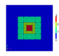
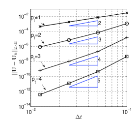
Refer to caption
Figure 6: Temporal refinement level
Refer to caption Refer to caption
Figure 7: Left: error 𝐔𝐔hL2(;𝐋2(Ω))subscriptnorm𝐔subscript𝐔subscript𝐿2subscript𝐋2Ω\|\mathbf{U}-\mathbf{U}_{h}\|_{L_{2}(\mathcal{I};\mathbf{L}_{2}(\Omega))}, right: error maxk𝐔(tk)𝐔h(tk)0,Ωsubscript𝑘subscriptnorm𝐔subscript𝑡𝑘subscript𝐔subscript𝑡𝑘0Ω\max\limits_{k}\|\mathbf{U}(t_{k})-\mathbf{U}_{h}(t_{k})\|_{0,\Omega} for the local hh-refinement with respect to time depicted in Fig.6

6.1.3 Broadband pulse in a waveguide

We consider a broadband pulse in a coaxial waveguide. The exact solution is

𝐄𝐄\displaystyle\mathbf{E} =1re(π(f2f1)(zt)/2)2sin(π(f1+f2)(zt))𝐞rabsent1𝑟superscript𝑒superscript𝜋subscript𝑓2subscript𝑓1𝑧𝑡22𝜋subscript𝑓1subscript𝑓2𝑧𝑡subscript𝐞𝑟\displaystyle=\frac{1}{r}e^{-(\pi(f_{2}-f_{1})(z-t)/2)^{2}}\sin(\pi(f_{1}+f_{2})(z-t))\mathbf{e}_{r}
𝐇𝐇\displaystyle\mathbf{H} =1re(π(f2f1)(zt)/2)2sin(π(f1+f2)(zt))𝐞φ.absent1𝑟superscript𝑒superscript𝜋subscript𝑓2subscript𝑓1𝑧𝑡22𝜋subscript𝑓1subscript𝑓2𝑧𝑡subscript𝐞𝜑\displaystyle=\frac{1}{r}e^{-(\pi(f_{2}-f_{1})(z-t)/2)^{2}}\sin(\pi(f_{1}+f_{2})(z-t))\mathbf{e}_{\varphi}.

Here r𝑟r, φ𝜑\varphi and z𝑧z denote the radial, azimuthal and axial coordinates respectively and 𝐞rsubscript𝐞𝑟\mathbf{e}_{r}, 𝐞φsubscript𝐞𝜑\mathbf{e}_{\varphi} and 𝐞zsubscript𝐞𝑧\mathbf{e}_{z} the corresponding unit vectors. The mid-frequency (f1+f2)/2subscript𝑓1subscript𝑓22(f_{1}+f_{2})/2 is chosen such that the corresponding wavelength is approximately 1/161161/16 the length of the waveguide. The spatial mesh consists of 1600 hexahedra with an edge-length of approximately 1/3λ13𝜆1/3\lambda. The global time step is fixed, such that in total 400400400 time steps are neccessary to propagate the pulse through the entire waveguide. In Fig. 8 we show the time trace of the spatial L2subscript𝐿2L_{2}-errors. The error exhibits an odd even pattern, the origin of which is yet unknown. We suspect this behavior to be related to the choice of a central flux. A similar behaviour is reported in [21].
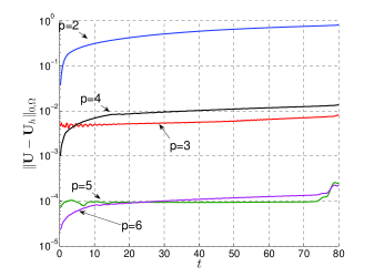
Refer to caption
Figure 8: Temporal evolution of the spatial L2subscript𝐿2L_{2}-error for p=2,3,4,5,6𝑝23456p=2,3,4,5,6

6.1.4 Bi-static RCS, metallic sphere - global p𝑝p-refinement

A metallic sphere of radius a=1𝑎1a=1 is illuminated by a 𝐞xsubscript𝐞𝑥\mathbf{e}_{x}-polarized plane wave traveling in ezsubscript𝑒𝑧e_{z}-direction with wave number ω=2π𝜔2𝜋\omega=2\pi. We chose ΩΩ\Omega as a spherical shell with outer radius R=5𝑅5R=5. For the outer boundary a Silver-Müller boundary condition is applied. The spatial grid consists of only 576 hexahedral elements with about 2 elements per wavelength at the surface of the scatterer and one element per wavelength at the absorbing boundary. The polynomial degrees are chosen as p=pt=px=py=pz=pgeo𝑝subscript𝑝𝑡subscript𝑝𝑥subscript𝑝𝑦subscript𝑝𝑧subscript𝑝𝑔𝑒𝑜p=p_{t}=p_{x}=p_{y}=p_{z}=p_{geo}, where pgeosubscript𝑝𝑔𝑒𝑜p_{geo} is the polynomial degree of the elemental mapping F𝐹F. We compute the bi-static RCS

σ(ϕ,θ)=limr4πr2|𝐄sc(r,ϕ,θ)|2|𝐄inc(r,ϕ,θ)|2𝜎italic-ϕ𝜃subscript𝑟4𝜋superscript𝑟2superscriptsubscript𝐄𝑠𝑐𝑟italic-ϕ𝜃2superscriptsubscript𝐄𝑖𝑛𝑐𝑟italic-ϕ𝜃2\displaystyle\sigma(\phi,\theta)=\lim\limits_{r\rightarrow\infty}4\pi r^{2}\frac{|\mathbf{E}_{sc}(r,\phi,\theta)|^{2}}{|\mathbf{E}_{inc}(r,\phi,\theta)|^{2}}

Here r𝑟r denotes the distance from the center of the sphere to the point of observation r𝐱𝑟𝐱r\mathbf{x}, ϕitalic-ϕ\phi and ϑitalic-ϑ\vartheta the azimuthal and polar angle between the wave and 𝐱𝐱\mathbf{x}. The scattered far field is evaluated at a closed surface S𝑆S, one wavelength away from the scatterer by evaluating the near-to-far field transformation

𝐄sc=eiωr4πrt0t1S[𝐱×(𝐱×(𝐧×𝐇h))+𝐱×(𝐄h×𝐧)]eiω𝐱𝐲iωtdS(𝐲)dtsubscript𝐄𝑠𝑐superscript𝑒𝑖𝜔𝑟4𝜋𝑟superscriptsubscriptsubscript𝑡0subscript𝑡1subscript𝑆delimited-[]𝐱𝐱𝐧subscript𝐇𝐱subscript𝐄𝐧superscript𝑒𝑖𝜔𝐱𝐲𝑖𝜔𝑡differential-d𝑆𝐲differential-d𝑡\displaystyle\mathbf{E}_{sc}=\frac{e^{-i\omega r}}{4\pi r}\int\limits_{t_{0}}^{t_{1}}\int_{S}\left[\mathbf{x}\times(\mathbf{x}\times(\mathbf{n}\times\mathbf{H}_{h}))+\mathbf{x}\times(\mathbf{E}_{h}\times\mathbf{n})\right]e^{i\omega\mathbf{x}\cdot\mathbf{y}-i\omega t}\,\mathrm{d}S(\mathbf{y})\,\mathrm{d}t

with Gauss quadrature of sufficiently high order. The computed RCS in Fig. 9 converge quickly to the analytical Mie-series solution.
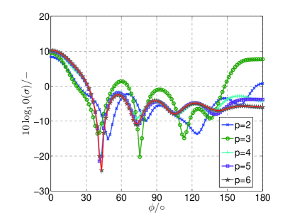
Refer to caption
Figure 9: Bi-static RCS, of a ka=2π𝑘𝑎2𝜋ka=2\pi PEC sphere, numerical solutions for a 576-element mesh with polynomial degrees p=2,,6𝑝26p=2,\ldots,6 and the analytical Mie-series solution (red)

6.2 Space-time hp𝑝hp-adaptive examples

In order to demonstrate the method’s capability for space-time hp𝑝hp-refinement, we propose an adaptive algorithm, which extends the concept of reference solutions [7, 22] to the space-time context.

  • 1.

    First a global time step ΔtΔ𝑡\Delta t, resulting in equally sized time slabs, is chosen.

  • 2.

    Given a time slab Δt×ΩΔ𝑡Ω\Delta t\times\Omega, an initial mesh 𝒮0subscript𝒮0\mathcal{S}_{0} and polynomial-degree distribution 𝐩0subscript𝐩0\mathbf{p}_{0}

  • 3.

    Define a coarse discretization (𝒮H,𝐩H)=(𝒮0,𝐩0)subscript𝒮𝐻subscript𝐩𝐻subscript𝒮0subscript𝐩0(\mathcal{S}_{H},\mathbf{p}_{H})=(\mathcal{S}_{0},\mathbf{p}_{0}) and a refined discretization (𝒮h,𝐩h)subscript𝒮subscript𝐩(\mathcal{S}_{h},\mathbf{p}_{h}) with finite element spaces VHsubscript𝑉𝐻V_{H} and Vhsubscript𝑉V_{h} respectively. The refined discretization is obtained by isotropically refining all space-time elements and increasing the polynomial degrees by one. Note that VHsubscript𝑉𝐻V_{H} is contained in Vhsubscript𝑉V_{h}.
    Then the following steps are performed iteratively

    1. (a)

      SOLVE: Solve the problem (3) on the coarse and fine discretizations.

    2. (b)

      ESTIMATE: Compute the error indicators η(n×K)=𝐔h𝐔HL2(n;𝐋2(Ω))𝜂subscript𝑛𝐾subscriptnormsubscript𝐔subscript𝐔𝐻subscript𝐿2subscript𝑛subscript𝐋2Ω\eta(\mathcal{I}_{n}\times K)=\|\mathbf{U}_{h}-\mathbf{U}_{H}\|_{L_{2}(\mathcal{I}_{n};\mathbf{L}_{2}(\Omega))} and the approximate error bound 𝐔h𝐔HL2(n;𝐋2(Ω))TOLsubscriptnormsubscript𝐔subscript𝐔𝐻subscript𝐿2subscript𝑛subscript𝐋2Ω𝑇𝑂𝐿\|\mathbf{U}_{h}-\mathbf{U}_{H}\|_{L_{2}(\mathcal{I}_{n};\mathbf{L}_{2}(\Omega))}\leq TOL stop and proceed to the next time slab. Otherwise,

    3. (c)

      MARK: Apply a fixed fraction marking strategy [23] based on the indicators η(n×K)𝜂subscript𝑛𝐾\eta(\mathcal{I}_{n}\times K)

    4. (d)

      REFINE: For each marked n×Ksubscript𝑛𝐾\mathcal{I}_{n}\times K, set up a list of refinement candidates VH,n×Kcand(n×K^,𝐩K)superscriptsubscript𝑉𝐻subscript𝑛𝐾candsubscript𝑛^𝐾subscript𝐩𝐾V_{H,\mathcal{I}_{n}\times K}^{\mathrm{cand}}(\mathcal{I}_{n}\times\hat{K},\mathbf{p}_{K}). In particular, we allow for all combinations of the following modifications of the discretization parameters:

      • i.

        raise/decrease the polynomial degrees px,py,pz,ptsubscript𝑝𝑥subscript𝑝𝑦subscript𝑝𝑧subscript𝑝𝑡p_{x},p_{y},p_{z},p_{t}

      • ii.

        isotropically hh-refine/derefine in the spatial directions

      • iii.

        increase/decrease the temporal refinement level

      In case of an refinement, which yields new space-time elements, we restrict the number of candidates by choosing identical polynomial degrees for each new element.
      Choose

      VH,n×K=argminVHcandS.T.ηηcand>0ηcandη#DOF(VHcand),ηcandsubscript𝑉𝐻subscript𝑛𝐾subscriptargminformulae-sequencesuperscriptsubscript𝑉𝐻cand𝑆𝑇𝜂superscript𝜂cand0superscript𝜂cand𝜂#𝐷𝑂𝐹superscriptsubscript𝑉𝐻candsuperscript𝜂cand\displaystyle V_{H,\mathcal{I}_{n}\times K}=\operatorname*{arg\,min}\limits_{V_{H}^{\mathrm{cand}}S.T.\eta-\eta^{\mathrm{cand}}>0}\frac{\eta^{\mathrm{cand}}-\eta}{\#DOF(V_{H}^{\mathrm{cand}})},\eta^{\mathrm{cand}}
      =𝐔hΠVhVHcand𝐔hL2(n;𝐋2(Ω))2absentsuperscriptsubscriptnormsubscript𝐔superscriptsubscriptΠsubscript𝑉superscriptsubscript𝑉𝐻candsubscript𝐔subscript𝐿2subscript𝑛subscript𝐋2Ω2\displaystyle=\|\mathbf{U}_{h}-\Pi_{V_{h}}^{V_{H}^{\mathrm{cand}}}\mathbf{U}_{h}\|_{L_{2}(\mathcal{I}_{n};\mathbf{L}_{2}(\Omega))}^{2}

      as the new local finite elements space, leading to a new global space VHsubscript𝑉𝐻V_{H}. Build a new Vhsubscript𝑉V_{h} from VHsubscript𝑉𝐻V_{H} and go back to SOLVE.

  • 4.

    Now, for the current time slab the final coarse and fine grid solutions have been obtained.

Remark1: The initial data for coarse- and fine-grid solves for the current time slab is taken as the L2subscript𝐿2L_{2}-projection of the refined solution Uhsubscript𝑈U_{h} from the previous time slab. Note that in the case of spatial derefinement with respect to the previous time slab, i.e. if the spatial part of the finite element space is not contained in the current one, there will be dissipation introduced by the projection. See [24], for a more detailed discussion. However the amount of dissipation introduced seemed to be negligible compared to the total error for the examples we have considered.
Remark2: If an iterative solver is applied, we can choose the coarse grid solution as starting point for solving the fine grid problem. We have observed, that this considerably cuts down the number of fine grid iterations.

6.2.1 Broadband pulse in coaxial waveguide

\psaxes[labels=none,ticks=none]-¿(-0.2,-0.2)(-0.2,-0.2)(1,1) pysubscript𝑝𝑦p_{y}pxsubscript𝑝𝑥p_{x}y𝑦yx𝑥x
Figure 10: Visualization of tensor product polynomials with degrees pxsubscript𝑝𝑥p_{x},pysubscript𝑝𝑦p_{y}

We have solved the example from 6.1.3 with the hp𝑝hp-adaptive algorithm. For the initial discretization we have chosen a coarse mesh consisting of 200 elements of degree pt=1,px=py=pz=0formulae-sequencesubscript𝑝𝑡1subscript𝑝𝑥subscript𝑝𝑦subscript𝑝𝑧0p_{t}=1,p_{x}=p_{y}=p_{z}=0. In Fig. 11 we visualize the coarse grid hp𝑝hp-discretization for time slab 86, by showing from top to bottom the electric field magnitude, the spatial polynomial discretization, using the tensor product visualization depicted in Fig. 10 and the temporal polynomial degree distribution. In axial direction, where the pulse has greater variation, spatial polynomial degrees are chosen to be larger than in radial direction. The temporal polynomial degrees are raised in the area where the pulse is situated. The temporal refinement level was not raised in any of the time slabs.
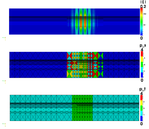
Refer to caption
Figure 11: Propagation of a broadband pulse in a cylindrical waveguide. From top to bottom: distribution of |𝐄h|subscript𝐄|\mathbf{E}_{h}|, (px,py,pz)subscript𝑝𝑥subscript𝑝𝑦subscript𝑝𝑧(p_{x},p_{y},p_{z}), and ptsubscript𝑝𝑡p_{t}

For the hp𝑝hp-adaptive solution we have obtained a relative fine-grid error in the norm L2(;𝐋2(Ω))\|\cdot\|_{L_{2}(;\mathbf{L}_{2}(\Omega))} of 9.6e39.6𝑒39.6e-3.

6.2.2 Scattering of a dielectric sphere

In the following, we consider the scattering of a Gaussian plane-wave by a dielectric sphere with ε=4𝜀4\varepsilon=4. The problem again was solved using the hp𝑝hp-adaptive algorithm. For the initial discretization we have chosen a coarse mesh consisting of 72 elements of degree pt=1,px=py=pz=0formulae-sequencesubscript𝑝𝑡1subscript𝑝𝑥subscript𝑝𝑦subscript𝑝𝑧0p_{t}=1,p_{x}=p_{y}=p_{z}=0. The discretization of time slabs 33, 65 and 124 (from top to bottom) is depicted in Fig. 12. The fact that the electric field has limited regularity at the material interface is reflected by the choice of moderate polynomial degrees in space and linear polynomial degrees in time and a comparatively small spatial mesh size near the material interface. Refinement in the temporal direction was almost exclusively hh-refinement, i.e. the temporal polynomial degree was almost exclusively equal to one. Thus we do not show the temporal polynomial degree distributions.
The bi-static RCS for ka=1𝑘𝑎1ka=1 is depicted in Fig. 13, where a relative 2subscript2\ell_{2}-error of 2.531022.53superscript1022.53\cdot 10^{-2} was obtained.

Refer to caption
Refer to caption
Refer to caption
Figure 12: hp𝑝hp-adaptive simulation of the scattering from a dielectric sphere. From left to right: distribution of |𝐄h|subscript𝐄|\mathbf{E}_{h}|, spatial polynomial degrees (px,py,pz)subscript𝑝𝑥subscript𝑝𝑦subscript𝑝𝑧(p_{x},p_{y},p_{z}) and temporal refinement level at timeslab 34, 66, 125 (from top to bottom)
Refer to caption
Figure 13: Bistatic RCS of a dielectric sphere with ε=4𝜀4\varepsilon=4 and ka𝑘𝑎ka=1, numerical solution (black circles), analytical Mie-series solution (red line)

7 Conclusions

We have devised a space-time Galerkin method, which allows for local hp𝑝hp-refinement in space and time by treating the spatial part of the discretization with a DG approach, wheras the temporal part is treated with a continuous Galerkin approach. The resulting implicit method can be shown to be non-dissipative, as long as the spatial part of the discretization is kept constant from time-slab to time-slab. We have shown, that the method can be implemented, such that the complexity of the residual evaluation for an iterative solution is 𝒪(p4)𝒪superscript𝑝4\mathcal{O}(p^{4}) for affine elements and 𝒪(p5)𝒪superscript𝑝5\mathcal{O}(p^{5}) for non affine elements. Furthermore, for the case of no local refinement with respect to time, we have devised an a posteriori bound on the iteration error. Thus a balancing of the iteration and discretization errors is possible, provided that an a posteriori estimate for the discretization error is available. While the presented method has higher computational costs than explicit hp-DG methods such as [24, 25], it provides the possibility to apply hp-adaptivity not only in space but also in time. It therefore allows to control the approximation error in the entire space-time domain of interest. We presented numerical experiments confirming that the method can be used for fully space-time hp-adaptive simulations.
The a priori and a posteriori error analysis is subject of ongoing work. Other future work should relate to the investigation of more efficient methods for the iterative solution of the linear systems, in particular regarding preconditioning.

References

References

Acknowledgements

The work of M. Lilienthal is supported by the ’Excellence Initiative’ of the German Federal and State Governments and the Graduate School of Computational Engineering at Technische Universität Darmstadt and the DFG under grant no. DFG WE 1239/27-2.
S.M. Schnepp acknowledges the support of the Alexander von Humboldt Foundation through a Feodor Lynen-Research Fellowship.
We thank Jens Niegemann for providing code for the computation of the Mie-series solutions.
We would like to thank Herbert Egger for giving valuable hints, which improved the presentation of the material significantly.