Single-exposure profilometry using partitioned aperture wavefront imaging

Abstract

We demonstrate a technique for instantaneous measurements of surface topography based on the combination of a partitioned aperture wavefront imager with a standard lamp-based reflection microscope. The technique can operate at video rate over large fields of view, and provides nanometer axial resolution and sub-micron lateral resolution. We discuss performance characteristics of this technique, which we experimentally compare with scanning white light interferometry.

Optical surface profiling is important in many applications ranging from precision optics to semiconductor industry. Currently, it is dominated by scanning white light interferometry (SWLI). In this approach, a surface profile is recovered from interferometric intensity variations recorded at a camera as a function of relative pathlength differences between sample and reference beams Flournoy_1972 ; Davidson_1987 ; Kino_1990 ; Wyant_1992 ; Wyant_2013 . The lateral resolution of the method is defined by the diffraction limit, which for visible light is a fraction of a micron. The axial resolution, approaching sub-nanometer range, is limited by noise in the system, such as shot noise, detector noise, or mechanical uncertainties in the relative pathlengths of the beams. In particular, the requirement of scanning in SWLI exacerbates the problem of mechanical uncertainties and limits applications to quasi-static profiling. Practical implementations of SWLI require precision mechanics which add to the cost of commercial devices.

In this work we describe a method of surface profiling that provides instantaneous measurements with resolution and dynamic range comparable to those of SLWI, yet characterized by a simple, robust and inexpensive design. The key element of our method is a Partitioned Aperture Wavefront (PAW) imager PAW , which is a passive add-on that can be incorporated into any standard widefield microscope. PAW imaging provides simultaneous phase and amplitude contrast that is quantitative. It has the advantages of being fast (single exposure), achromatic (works with lamp or LED illumination), and light efficient (works with extended sources). We previously demonstrated an implementation of PAW imaging in a transmission microscope configuration to measure the phase shifts induced by biological cells on a slide PAW . Here, we implement PAW imaging in a reflection microscopy configuration to measure surface topography. We describe the performance of this device, which we compare with SWLI.

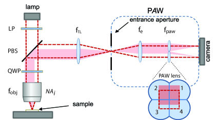
Figure 1: (color online) Experimental setup: $f_{\rm{obj}}$, $f_{\rm{TL}}$, $f_{e}$, and $f_{\rm{paw}}$ denote a microscope objective and lenses. A linear polarizer (LP), quarter-wave plate (QWP), and polarizing beam splitter (PBS) minimize spurious back-reflections. The 3f PAW module includes a composite lens (inset) that projects four oblique-detection images onto a camera.

PAW imaging is based on partitioning the detection aperture of a standard imaging device into four quadrants, similarly to pyramidal wavefront imaging Iglesias_2011 but with the difference that the partitioning is performed by four off-axis achromatic lenses rather than four prisms. These lenses provide four oblique-detection images that are simultaneously acquired with a single camera. The different perspectives presented by the four images enable the reconstruction of wavefront phase and amplitude with a simple numerical algorithm that runs in real time (here video rate).

Figure 1 illustrates an implementation of PAW imaging in a reflection configuration suitable for surface profilometry. This implementation consists of a standard reflection microscope based on Köhler illumination with an illumination numerical aperture $\rm{NA}_{i}$. The microscope camera, normally located at the intermediate image plane, is set back to allow the insertion of the PAW module. This relays the intermediate image through a 3f imaging system comprising an entrance lens of focal length $f_{e}$ and the composite PAW lens. The latter consists of four off-axis lenses of focal length $f_{\rm{paw}}$, cut and glued together in a quatrefoil geometry (see Fig. 1 inset). A square entrance aperture is placed in the intermediate image plane to prevent overlapping of the four images at the camera plane. This square aperture defines the system field of view (FOV).

The principle of surface profilometry based on PAW imaging can be understood from simple geometrical optics (see Fig. 1). Let us first consider a flat reflective sample orthogonal to the optical axis. Provided the illumination source is symmetrically distributed about the optical axis, the illumination rays incident on the sample are, on average, normal to the sample plane. The reflected rays are thus also, on average, normal to the sample surface, and the power through the four PAW lenses is distributed equally (dashed lines). That is, the four recorded images are of equal uniform intensity. Let us now consider a local slope in the sample profile. This leads to a local off-axis tilting of the reflected rays, and hence to an unbalancing of the power distribution through the PAW lenses (shaded). The local intensity differences in the recorded images thus encode local slope variations in the sample surface profile.

These considerations, applicable in the paraxial approximation, suggest the basic reconstruction algorithm for surface profiling. Specifically, in the case of a square illumination aperture used in our work, the local tilt angles along the transverse axes are defined by the simple algebraic combinations  Iglesias_2011 ; PAW :

$$\theta_{x} = {\rm{NA}_{i}}\left(I_{1}-I_{2}-I_{3}+I_{4}\right)/I_{\rm tot},$$

$$\theta_{y} = {\rm{NA}_{i}}\left(I_{1}+I_{2}-I_{3}-I_{4}\right)/I_{\rm tot},$$ (1)

where $I_{k}$ are the image intensities recorded in the four quadrants of the camera (see Fig. 1), and $I_{\rm tot}=\sum_{k=1}^{4}I_{k}$ is the total intensity, equivalent to a standard widefield image of the sample. Provided the detection numerical aperture $\rm{NA}_{d}$ is at least twice $\rm{NA}_{i}$, then Eqs. (Single-exposure profilometry using partitioned aperture wavefront imaging) are accurate for tilt angles $|\theta_{x,y}|\leq\rm{NA}_{i}$, characterizing the dynamic range of the tilt measurements.

Physically, the tilt angles (Single-exposure profilometry using partitioned aperture wavefront imaging) encode surface gradients,

$$\theta_{x}=2\nabla_{x}h,\quad\theta_{y}=2\nabla_{y}h,$$ (2)

where $h=h({\boldsymbol{\rho}})$ is the surface profile at the position ${\boldsymbol{\rho}}=(x,y)$ in the sample, and the factor of two accounts for the doubling of the reflected angle with respect to the surface normal.

Surface profile is reconstructed by integration of Eq. (2), which we perform using a spiral phase Fourier integration method described in Ref. Arnison_2004 . In the continuum limit we have

$$h({\boldsymbol{\rho}})-h_{0} = \frac{1}{4\pi i}\int d^{2}{\boldsymbol{\kappa}}\,e^{i2\pi{\boldsymbol{\kappa}}\cdot{\boldsymbol{\rho}}}\,\frac{\tilde{\theta}({\boldsymbol{\kappa}})}{\kappa_{x}+i\kappa_{y}},$$ (3)

where ${\boldsymbol{\kappa}}=(\kappa_{x},\kappa_{y})$ is a spatial frequency, $h_{0}$ is an arbitrary constant, and we introduce a complex function $\theta({\boldsymbol{\rho}})=\theta_{x}+i\theta_{y}$, with Fourier transform $\tilde{\theta}({\boldsymbol{\kappa}})$. This integration method implicitly assumes that the spatial support of $\theta({\boldsymbol{\rho}})$ is finite. That is, we assume that the average global tilt of the sample is zero. In practice one can always balance and zero-pad the recorded quadrant images to satisfy this condition Bon_2012 . Global tilts given by $\overline{\theta}_{x}$ and $\overline{\theta}_{y}$, should they exist, may be derived separately from the average relative intensities of the quadrant images and found by direct integration of Eq. (2), leading to a baseline surface tilt $h^{\rm{base}}({\boldsymbol{\rho}})-h_{0}=\overline{\theta}_{x}x+\overline{\theta}_{y}y$. This tilt may then be added to the local profile variations found by Eq. (3), leading to a full solution for $h({\boldsymbol{\rho}})$.

In a previous publication PAW we concentrated on high resolution imaging at the diffraction limit defined by a relatively large $\rm{NA}_{i}=0.45$. In this work, we focus instead on another feature of PAW imaging, namely its capacity to readily image over large FOVs. For this, we will employ small $\rm{NA}_{i}$’s. This has the advantage of providing large depth of fields (DOFs), meaning that surface height variations $h({\boldsymbol{\rho}})$ can be measured over long ranges in a single exposure (i.e. without having to readjust $h_{0}$). A disadvantage of large FOVs, however, is that our lateral resolution is likely to be pixel limited rather than diffraction limited. We must therefore properly account for pixel-induced spatial filtering of the recorded images, which in turn leads to a spatial filtering of $\theta({\boldsymbol{\rho}})$ in Eq. (Single-exposure profilometry using partitioned aperture wavefront imaging). Such filtering is written as a convolution $\theta^{s}({\boldsymbol{\rho}})={\rm P}({\boldsymbol{\rho}})\otimes\theta({\boldsymbol{\rho}})$, where ${\rm P}({\boldsymbol{\rho}})$ is the normalized spatial filter corresponding to a single pixel, and we assume that the total intensity $I_{\rm tot}$ varies slowly over the scale of a pixel (recall that for pure phase samples $I_{\rm tot}$ is uniform). For a square pixel of projected size $p$ at the sample plane, one obtains ${\rm\tilde{P}}({\boldsymbol{\kappa}})={\rm sinc}(\kappa_{x}p)\,{\rm sinc}(\kappa_{y}p)$, where ${\rm sinc}(x)=\sin(\pi x)/(\pi x)$, leading to the required modification of the kernel in Eq. (3): $\kappa_{x}+i\kappa_{y}\to(\kappa_{x}+i\kappa_{y}){\rm sinc}(\kappa_{x}p)\,{\rm sinc}(\kappa_{y}p)$. A similar modification can be found in Ref. Arnison_2004 , though arising from a different consideration of image shear rather than pixel size.

At first glance it might appear that any phase retrieval technique based on the integration of phase gradients would be susceptible to measurement errors that propagate upon integration. This is not the case here for two reasons. First, the spiral phase Fourier integration defined by Eq. (3) dampens the propagation of error (more on this below). Second, sharp phase gradients that would normally lead to measurement error because they fall outside our dynamic range (i.e. $|\theta_{x,y}|>{\rm{NA}}_{i}$), in fact, do not because they are largely smoothed over by the limited spatial resolution of our device. As an example, let us consider a sample that features a sharp phase step as depicted in Fig. 2. In the case where the spatial resolution of our device is diffraction limited ($\approx\lambda/(2{\rm{NA}}_{i})$), the reconstructed phase profile, taking this resolution into account, exhibits slight ringing but otherwise remains accurate over the scale of the resolution (provided the phase step is not larger than $\lambda/2$ over this scale). In the case where the spatial resolution is pixel limited, the error may or may not be worsened depending on the exact location of the phase step relative to the pixel array, as illustrated in Fig. 2, but here too the error remains fairly well localized to within a few pixels of the step. Our phase retrieval method is thus highly robust.

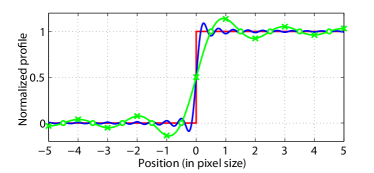
Figure 2: (color online) Step profile discontinuity in sample (red), and simulated profile reconstruction when system resolution is diffraction limited (blue) or pixel limited with $\times 2$ undersampling (green). $\circ$ and $\times$ indicate representative pixel array positions relative to the step discontinuity.

Our experimental setup is shown in Fig. 1. The illumination source was an LED with center wavelength $\lambda=525\,{\rm nm}$ and bandwidth $\sim 20\,{\rm nm}$ (Thorlabs). Two standard Olympus objectives with magnification 10$\times$ ($\rm{NA}=0.25$) and 1.25$\times$ ($\rm{NA}=0.04$) were used for medium and low magnification measurements, respectively. The total system magnification $M_{\rm tot}$ was defined by the microscope tube lens $f_{\rm{TL}}=150\,{\rm mm}$, and the PAW module lenses $f_{e}=150\,{\rm mm}$ and $f_{\rm{paw}}=50\,{\rm mm}$. $\rm{NA}_{i}$ was defined by the size of a square aperture $d_{i}=3.5\,{\rm mm}$ imaged onto the objective back apertures, obtaining $M_{\rm tot}=2.8\times$, $\rm{NA}_{i}=0.097$ and $\rm{DOF}=28.0\,{\rm\mu}m$ for the 10$\times$ objective, and $M_{\rm tot}=0.35\times$, $\rm{NA}_{i}=0.012$ and $\rm{DOF}=1.8\,{\rm mm}$ for the 1.25$\times$ objective. As a detector we employed a 10-bit machine-vision CCD camera (Hitachi KP-F120) with square pixels $6.45\,{\rm\mu m}$ in size, capable of acquiring images at 30 fps.

As described, our profilometer cannot distinguish tilt angles $\theta_{x,y}$ induced by the sample from those induced by system aberrations. To correct for the latter, we first obtained reference quadrant images $I^{\rm{ref}}_{k}$ from a simple flat mirror, which, ideally, should be uniform and of equal intensities. In practice, however, they contained variations due to system aberrations. This reference measurement need only be performed once for each setup configuration. Subsequent sample images $I^{\rm{sample}}_{k}$ were then normalized according to

$$I_{k}=I^{\rm{sample}}_{k}/I^{\rm{ref}}_{k},\quad k=1..4.$$ (4)

As noted above, any small misalignment of the reference mirror from normal, as evidenced by a slight imbalance in the reference quadrature intensities, does not affect our reconstruction of sample surface variations.

To characterize the performance of our device, we chose a well defined sample that could be dynamically varied and controlled, namely a deformable mirror (DM) provided by Boston Micromachines Corp. The mirror consisted of $140$ reflective elements which could be individually controlled at an update rate of $3\,{\rm kHz}$, forming a grid of period $400\,{\rm\mu m}$ with maximum stroke about $2\,{\rm\mu m}$. As a test profile, we imposed a two-dimensional checkerboard pattern. The resulting normalized quadrature images obtained with the 10$\times$ objective are shown in Fig. 3.

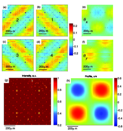
Figure 3: (color online) Images of DM obtained after correcting for system aberrations according to Eq. (4): (a-d) Quadrant images $I_{1..4}$ (a.u.) recorded by camera, with dc level subtracted for ease of presentation; (e-f) calculated light tilts $\theta_{x}$ and $\theta_{y}$ (a.u.); (g) normalized widefield image $I_{\rm tot}$ (note apparent supporting structure and etch-access holes); (h) profile of the DM with color-encoded height ($\mu m$).

To verify the accuracy of our surface height measurements, we compared our results with those obtained by a commercial profilometer based on SWLI (Zygo NewView 6300). The results are shown in Fig. 4, where the FOVs from both instruments were scaled and cropped to be identical. The color bar encodes the reconstructed profile in microns (with average height set to zero), depicting height variations in the range of about $1\,{\rm\mu m}$. The agreement between the two techniques is excellent, with root-mean square discrepancies not exceeding $20\,{\rm nm}$ over the entire FOV. As expected, we observe the largest discrepancies close to the etch-access holes in the DM where the surface height variations vary rapidly. Again, these discrepancies are local only, and can be readily identified from the widefield image $I_{\rm tot}$.

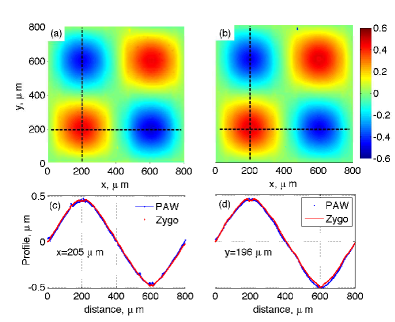
Figure 4: (color online) Profiles of DM reconstructed by (a) PAW and (b) SWLI, and representative line profiles (c,d) for comparison.

We note that a key difference between PAW and SWLI profilometry is that PAW can provide measurements at video rate compared to the several seconds typically required by SWLI. Another key difference is the ready capacity of PAW to operate over large FOVs. By simply switching to the 1.25$\times$ objective (and recalibrating), we extended the FOV eight-fold from $800\,{\rm\mu m}$ to $6.5\,{\rm mm}$. In this manner, we were able to acquire a surface profile of the entire DM active area, as illustrated in Fig. 5, again at video-rate.

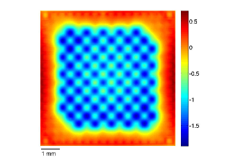
Figure 5: (color online) Profile of entire DM surface (color encoded in $\mu m$) imaged at low magnification and reconstructed by PAW.

Finally, we consider the noise characteristics of our device. In particular, we evaluate the uncertainty in our height measurements arising from unavoidable sources such as shot noise and camera readout noise. Equation (3) can be recast as $\langle h({\boldsymbol{\rho}})\rangle-h_{0}=K({\boldsymbol{\rho}})\otimes\langle\theta({\boldsymbol{\rho}})\rangle$, where $K({\boldsymbol{\rho}})=(x-iy)/4\pi\rho^{2}$ and $\langle...\rangle$ indicates an average over multiple measurements. Provided light tilt fluctuations $\delta\theta=\theta-\langle\theta\rangle$ are locally uncorrelated, we have $\langle\delta\theta({\boldsymbol{\rho}}_{1})\delta\theta^{*}({\boldsymbol{\rho}}_{2})\rangle=p^{2}\sigma^{2}_{\theta}\delta^{2}({\boldsymbol{\rho}}_{1}-{\boldsymbol{\rho}}_{2})$, where $\delta^{2}({\boldsymbol{\rho}})$ is a 2D delta function, and the variance $\sigma^{2}_{\theta}=\langle\delta\theta^{2}({\boldsymbol{\rho}})\rangle$ is independent of position ${\boldsymbol{\rho}}$. This variance can be derived from Eq. (Single-exposure profilometry using partitioned aperture wavefront imaging) and is given by PAW

$$\sigma^{2}_{\theta}=\sigma^{2}_{\theta_{x}}+\sigma^{2}_{\theta_{y}}=2{\rm{NA}}^{2}_{i}\left[4\sigma_{r}^{2}+I_{\rm tot}\right]/I^{2}_{\rm tot},$$ (5)

where $I_{\rm tot}$ is measured in photoelectrons, $\sigma^{2}_{r}$ is the camera readout noise variance, and we assume that the average light tilts are much smaller than ${\rm{NA}}_{i}$.

The variance of the surface profile $\sigma^{2}_{h}=\langle\delta h^{2}({\boldsymbol{\rho}})\rangle$ is thus approximated by

$$\sigma_{h}^{2} \approx \frac{p^{2}\sigma^{2}_{\theta}}{8\pi}\ln(N/2),$$ (6)

where $N$ is the FOV in pixel counts. The logarithmic dependence on FOV arises from the long-range behavior of the kernel $K({\boldsymbol{\rho}})$. Because this decays according to a power law, which is largely confined, the dependence on FOV is weak. From Eq. (6) we expect theoretically $\sigma_{h}^{\rm{th}}\approx 3\,{\rm nm}$, which is close to the experimentally measured $\sigma_{h}^{\rm{exp}}\approx 2\,{\rm nm}$.

In summary, we have developed an optical surface profiling technique that can provide video-rate measurements of dynamic samples, featuring diffraction-limited lateral resolution and nanometric axial resolution comparable to SWLI. The technique can be implemented as a simple add-on to a standard lamp-based reflection microscope, making it an attractive and inexpensive alternative to SWLI.

We thank T. Bifano, J.-C. Baritaux and T. N. Ford for helpful discussions, and Boston Micromachines Corp. for providing a DM. This work was supported by the BU Photonics Center through a NSF I/UCRC grant.

References

- (1) P. A. Flournoy, R. W. McClure, and G. Wyntjes, Appl. Opt. 11, 1907-1915 (1972).
- (2) M. Davidson, K. Kaufman, I. Mazor, and F. Cohen, Proc. SPIE 775, 233 (1987).
- (3) G. S. Kino and S. C. Chim, Appl. Opt. 29, 3775 (1990).
- (4) J. C. Wyant and K. Creath, Int. J. Mach. Tools Manufact. 32, 5 (1992).
- (5) J. C. Wyant, Appl. Opt. 52, 1 (2013).
- (6) A. B. Parthasarathy, K. K. Chu, T. N. Ford, and J. Mertz, Opt. Lett. 37, 4062 (2012).
- (7) I. Iglesias, Opt. Lett. 36, 3636 (2011).
- (8) M. R. Arnison, K. G. Larkin, C. J. R. Sheppard, N. I. Smith, and C. J. Cogswell, J. Microsc. 214, 7 (2004).
- (9) P. Bon, S. Monneret, and B. Wattellier, Appl. Opt. 51, 5698 (2012).
- (10) F. Gao, R. K. Leach, J. Petzing, and J. M. Coupland, Meas. Sci. Technol. 19, 015303 (2008).