Spatial volume dependence for 2+1 dimensional SU(N) Yang-Mills theory

Abstract:

We study the 2+1 dimensional SU(N) Yang-Mills theory on a finite two-torus with twisted boundary conditions. Our goal is to study the interplay between the rank of the group $N$, the length of the torus $L$ and the $Z_{N}$ magnetic flux. After presenting the classical and quantum formalism, we analyze the spectrum of the theory using perturbation theory to one-loop and using Monte Carlo techniques on the lattice. In perturbation theory, results to all orders depend on the combination $x=\lambda NL$ and an angle $\tilde{\theta}$ defined in terms of the magnetic flux ($\lambda$ is ‘t Hooft coupling). Thus, fixing the angle, the system exhibits a form of volume independence ($NL$ dependence). The numerical results interpolate between our perturbative calculations and the confinement regime. They are consistent with x-scaling and provide interesting information about the k-string spectrum and effective string theories. The occurrence of tachyonic instabilities is also analysed. They seem to be avoidable in the large N limit with a suitable scaling of the magnetic flux.

1 Introduction

Yang-Mills theories are a fantastic laboratory to test our understanding of quantum field theory: very simple to formulate, but containing a extremely rich phenomenology. Despite the enormous progress made, we are not yet at the level of claiming a full understanding of many of the entailing phenomena, such as confinement. Although most of the phenomenological interest lies in 3+1 space-time dimensions, the 2+1 case has also been subject of interest. Proving confinement is not so much of a challenge in that case, because even the abelian theories with monopoles enjoy this property in 2+1 dimensions [1]. However, we still face the challenge of having a successful computational method to provide the full spectrum of the theory. No doubt that the lattice approach [2] provides numerical values for the string tension and spectrum [3]. Nevertheless, it would be very desirable to have semi-analytical approaches that could provide approximate results and a deep understanding of the relevant dynamics involved. From that point of view, the 2+1 case, being simpler, is also a perfect laboratory for ideas, methods and techniques applicable to the higher dimensional case and to other theories. There is an extensive literature on the subject where these ideas have been put forward. For example, we signal out the work done by Nair, who proposed an approach which can lead to the desired analytical control [4].

The present work started with the concrete goal of analyzing the interplay between the dependence of the theory on the rank of the gauge group $N$ and on the volume of space-time. Both dependencies are presumably strongly linked to each other. The intriguing connection among both quantities (rank and volume) was initially put forward by Eguchi and Kawai [5]. In particular, it was suggested that when the rank of the group goes to infinity, finite volume effects vanish. However, the validity of this result, often called large N reduction, rests upon assumptions about whether certain symmetries are unbroken. As a matter of fact, the single lattice point reduced model proposed in Ref. [5] was soon disproved [6] due to breaking of the necessary $Z(N)^{4}$ symmetry. Two possible ways out were soon proposed; one in Ref. [6] and the other in Refs. [7, 8].

Here we will not be directly concerned with the reduced models. We will adopt a more general viewpoint, and simply consider the dynamics of SU(N) Yang-Mills fields living on a finite spatial manifold but in infinite (euclidean) time. This is an appropriate setting for a Hamiltonian description in which the spectrum of the system can be studied. In particular, we will choose the spatial manifold to be a two-torus with euclidean metric and size $L_{1}\times L_{2}$. The choice of the torus allows the introduction of a certain topology in the space of SU(N) gauge fields through the selection of the boundary conditions. This was first realized by ‘t Hooft [9], and following his nomenclature, they are called twisted boundary conditions. In this particular 2-dimensional situation, they are associated to the introduction of a discrete modulo N magnetic flux through space. Boundary conditions have a strong impact on the finite volume dynamics at weak coupling. This is the reason why in Ref. [7, 8] it was proposed that using twisted boundary conditions the reduction idea could be rescued. The corresponding reduced model is hence known as the twisted Eguchi-Kawai model (TEK). Here, we will not attempt a full description of the model and a review of its properties, since as mentioned previously, our approach is more general. It is nevertheless necessary to comment some aspects of the history of reduced models in as much as it affects the selection of our framework.

Already in Ref. [8] and in Ref. [10] an alternative derivation of reduction was given based on perturbation theory within the twisted reduction scheme. Despite the absence of spatial degrees of freedom, a suitable description of the Lie algebra mimics the Fourier expansion on a finite lattice. The Feynman rules remember the non-commutative nature of the group through the presence of momentum dependent phases in place of the structure constants of the group. These phases have an important effect in selecting planar diagrams over the rest. Indeed, only for planar diagrams the overall phases of a diagram cancel, as proven in the aforementioned references and in Ref. [11]. The peculiar Feynman rules were encountered, perhaps not unsurprisingly, many years later in the context of quantum field theories on non-commutative space (for a review see [12]). Indeed, the presence of momentum dependent phases has little to do with the lattice nature of the TEK model. A continuum version of the rules was given very early [13], having an obscure interpretation until its reappearance in the context of non-commutative space. The quick development of the field following its appearance in the string theory literature led to the identification of problems within the perturbative regime. These manifest themselves in that the negative character of the self-energy makes certain low momentum modes become tachyonic, signalling the instability of the perturbative vacuum [14]-[19]. The fate of the model has to be addressed non-perturbatively [20] and in this respect the TEK model played a role as a regulated version of the non-commutative theory [21].

Apart from the afore-mentioned problems, numerical studies [22, 23, 24] showed the appearance of symmetry breaking for the TEK model at large values of $N$. This was interpreted as a first order transition to a symmetry breaking vacuum configuration which at small coupling appears as a metastable state. The connection between these problems and the ones mentioned previously in relation with tachyonic instability remains unclear. In any case, the previously mentioned interpretation of the origin of the problem in terms of metastable states, allowed to find a solution. It turns out [25] that, rather than keeping the integer magnetic flux associated to twist fixed as the rank of the group $N$ goes to infinity, one has to scale this flux in a concrete way with $N$. This prescription has led to results which are not only free of symmetry breaking, but also reproduce the results obtained by direct extrapolation to large N in a rather spectacular way [26]. Despite the numerical success, it is clear that a deeper understanding is welcome. The present paper, which addresses the 2+1 dimensional case, is a step in that direction. The lesson to be learned is that particular care has to be paid to the dependence on the total magnetic flux and its scaling properties with N.

Up to now our motivation has been centered upon large N physics, however, the interest of volume dependence at finite N is also relevant for other purposes. Certainly, from a practical point of view, since non-perturbative results obtained on the lattice are subject to these corrections. From a more fundamental standpoint the use of the space-time volume was advocated as a good parameter to monitor the transition from the small box perturbative region to the large volume confinement regime. This program had the goal of providing new calculational techniques or new insights into the nature of non-perturbative phenomena [27, 28]. Here, of course, boundary conditions do matter, and the use of twisted boundary conditions was argued to produce a smoother transition in several perturbative [29, 30, 31] and non-perturbative works [32, 33]. It has also been advocated as a tool to determine the electric-flux spectrum and employed to analyze the confinement/deconfinement transition [34]-[36]. To conclude this lengthy motivation we should mention that recently a fundamental line of work has also advocated the use of spatial size as a monitoring parameter with a similar goal of developing new calculational techniques and/or insights into the nature of some non-perturbative phenomena [37, 38]. In the majority of these new works only one direction is kept finite and, in the absence of a phase transition, it allows to continuously connect to a dimensionally reduced model, benefiting from the use of the powerful low-dimensional techniques available.

After having put our work in perspective and motivated its interest, we address the description of the lay-out of the paper. As mentioned earlier we will focus upon SU(N) Yang-Mills theory living on a $T_{2}\times R$, space-time. We will restrict ourselves to the case in which the fields satisfy twisted boundary conditions with non-zero magnetic flux $m$ on the spatial two-torus of size $L_{1}\times L_{2}$. The case of periodic boundary conditions demands very different techniques and has been studied more extensively earlier both in the papers mentioned before [27, 28], as in the context of large N reduction [39]. Our paper is neatly divided into three parts. The first part develops the formalism. Since few researchers are acquainted with this formalism, we have made an effort to make a self-contained presentation that could serve as background material for this and future papers. The 2+1 dimensional case, being simpler, provides a good starting point before facing the more involved 3+1 case. The presentation begins with classical aspects exhibiting the two most useful types of partial gauge fixing. One of the formulations is particularly well-suited for perturbative calculations, while the other is useful for semiclassical contributions around non-trivial minima of the action. The connection of these two formalisms is a new result, whose derivation is given in Appendix A. The quantization of the system is done in the Hamiltonian formalism in the $A_{0}=0$ gauge, where the Gauss constraint condition is implemented as a condition on physical states.

The second part proceeds by setting up the perturbative calculation of the spectra up to order $g^{2}$. The whole set of rules depends on the size of the torus $L$, the rank of the group $N$, the gauge coupling, better expressed as ‘t Hooft coupling $\lambda=g^{2}N$, and an angle $\tilde{\theta}$ which depends on the magnetic flux through space. We observe, that for fixed value of this angle all the size dependence appears in the combination $LN$ (for $L\equiv L_{1}=L_{2}$). This can be considered a strong form of reduction, which is valid at finite $N$. If, as expected, the zero-electric flux sector of the theory at large $NL$ becomes independent of this angle, this would imply the standard large $N$ reduction result. In this paper we focus specifically on the calculation of the lowest energy states in each electric flux sector. The most crucial part of the calculation is the one loop gluon self-energy contribution. In the Hamiltonian formalism this result appears as a sum of three individually divergent contributions. The divergence is however $\tilde{\theta}$ independent, so that the $\tilde{\theta}$ dependence of the self-energy can be easily derived. To extract a full finite result one must take care to regularize the expressions in a gauge invariant way. For that purpose we decided to calculate this self-energy following two additional gauge invariant procedures. The first being the calculation of the vacuum polarization in euclidean space, which later is dimensionally regularised. The result turns out to be finite and gives a $\tilde{\theta}$ dependence which coincides with the one computed earlier in the Hamiltonian formulation. Finally, we also use a lattice regularization. The result extrapolated to vanishing lattice spacing is again finite and coincides with the previous calculation. The whole result is summarised in an elegant self-energy formula which allows us to study the occurrence or not of tachyonic instabilities in the theory. Indeed, the formula always predicts negative energies for sufficiently large values of the coupling $\lambda$. The problem is that for certain choices of the magnetic flux, as the rank of the group gets larger, the coupling at which the instability occurs is small enough to validate the perturbative calculation. On the contrary, if we scale the magnetic flux with $N$, following the prescription of Ref. [25] generalized to 2+1 dimensions, the instabilities occur always at finite values of $\lambda$ at which the perturbative calculation is not necessarily trustworthy. This result is by itself one of the most important new results contained in our paper.

The previous considerations bring us naturally to the third part of the paper which makes use of the numerical study of the model discretized on the lattice. Our numerical results are far from being a complete test of the model, but were specifically designed to test the transition of the ground state energies from the region where the perturbative formulas should apply to that in which these energies enter the confinement regime giving rise to the linearly rising $k$-string spectrum, which will be analyzed. Our results provide non-perturbative support to the strong reduction conjecture indicating that the effective size controlling the linear growth of the k-string energies is indeed $LN$ or, more specifically, the dimensionless variable $x=\lambda LN/4\pi$. The dependence on $x$ and $\tilde{\theta}$ of the numerical results is fairly well described by a parameterization that encodes both the perturbative and the large volume asymptotic behaviour, including subleading terms in the effective string description of the electric-flux energies. This formula allows to extend the analysis of the appearance of tachyonic instabilities outside the realm of perturbation theory, and to argue that the prescription of Ref. [25] gives rise to non-tachyonic results in all the range of values of $x$.

The paper closes with a summary of our results and a description of open problems and future prospects.

2 Yang-Mills fields on a twisted box

This section will review the basic formalism for describing gauge fields living on a spatial torus. Here, we will be specific to the two-dimensional case in a Hamiltonian framework and will derive several formulas specific for this case. Most of the original papers developing the formalism have been cited in the introduction. Additional references and a more complete presentation to the field can be found in Ref. [40].

The first step is to define the configuration space. This is given by gauge fields on the torus. Namely, we have to define a bundle with base space the 2-torus and a connection on this bundle. The torus has euclidean metric and periods given by $L_{i}\hat{e}_{i}$, where $\hat{e}_{i}$ is the unit vector in the $i$th direction and $i=1,2$. As is customary in the Physics literature, we will work with a trivialization of the bundle entailed by having a single rectangular patch of size $L_{1}\times L_{2}$ and transition functions $\Omega_{i}(x)$. We will also take the bundle to be an SU(N) associated bundle in the fundamental representation. Hence, the transition matrices are $N\times N$ matrices. The consistency conditions imply:

$$\Omega_{1}(x+L_{2}\hat{e}_{2})\Omega_{2}(x)=e^{2\pi ik/N}\Omega_{2}(x+L_{1}\hat{e}_{1})\Omega_{1}(x)\quad,$$ (1)

where $k$ is an integer modulo $N$, known as magnetic flux. Once the bundle is trivialized the connection is given by the $N\times N$ traceless hermitian matrix $A_{i}(x)$. The periodicity condition for this connection is

$$A_{i}(x+L_{j}\hat{e}_{j})=\Omega_{j}(x)A_{i}(x)\Omega^{\dagger}_{j}(x)+i\Omega_{j}(x)\partial_{i}\Omega^{\dagger}_{j}(x)\quad.$$ (2)

The starting field-space of the system is given by the pair $\{\Omega_{i}(x),A_{i}(x)\}$. However, the physical configuration space is the space of trajectories under local gauge transformations. A gauge transformation acts on the starting space as follows:

$$A_{i}(x) \longrightarrow \Omega(x)A_{i}(x)\Omega^{\dagger}(x)+i\Omega(x)\partial_{i}\Omega^{\dagger}(x)\quad,$$ (3)

$$\Omega_{i}(x) \longrightarrow \Omega(x+L_{i}\hat{e}_{i})\Omega_{i}(x)\Omega^{\dagger}(x)\quad.$$ (4)

Wilson loops and Polyakov lines are gauge invariant observables, as well as the eigenvalues of the magnetic field.

We might partially constrain gauge transformations by fixing the value of $\Omega_{i}(x)$. Thus, gauge transformations should satisfy the following periodicity condition

$$\Omega(x+L_{i}\hat{e}_{i})=\Omega_{i}(x)\Omega(x)\Omega^{\dagger}_{i}(x)\quad.$$

There is a symmetry of the action corresponding to a transformation which multiplies the transition matrices by an element of $\mathbf{Z}_{N}$ without affecting the gauge field $A_{i}(x)$. This is not a gauge transformation since the Polyakov loops are multiplied by an element of the center. ‘t Hooft called them singular gauge transformations. Once we fix the gauge to specific transition matrices $\Omega_{i}(x)$, the symmetry transformation looks as an ordinary gauge transformation satisfying the following generalized periodicity condition

$$\Omega(x+L_{i}\hat{e}_{i})=e^{2\pi ik_{i}/N}\Omega_{i}(x)\Omega(x)\Omega^{\dagger}_{i}(x)\quad.$$ (5)

The space of x-dependent SU(N) matrices satisfying the previous equation will be labelled ${\cal G}(\vec{k})$. The quotient group

$$\left(\cup_{\vec{k}}\,{\cal G}(\vec{k})\right)/{\cal G}(\vec{0})\sim Z_{N}^{2}$$

is a very important symmetry group of our problem. Its representations are labelled by the electric flux vector $\vec{e}$.

We might generalize the periodicity condition for $\Omega(x)$ (Eq. 5) to arbitrary $N\times N$ matrices. This defines the vector spaces of matrix-valued fields ${\cal E}(\vec{k})$. These are interesting spaces satisfying

$$\forall U\in{\cal E}(\vec{k})\quad{\rm and}\quad V\in{\cal E}(\vec{k}^{\prime})\quad{\rm then}\quad UV\in{\cal E}(\vec{k}+\vec{k}^{\prime})\quad.$$ (6)

These spaces admit ${\cal G}(\vec{k})$ as subspaces. Even more, one can take a non-singular matrix $U(x)$ in ${\cal E}(\vec{k})$ and decompose it uniquely as a product

$$U=\Omega H\quad,$$ (7)

where $\Omega\in{\cal G}(\vec{k})$ and $H$ is hermitian and positive definite. Furthermore, $H$ belongs to ${\cal H}_{0}$, which is the subspace of ${\cal E}(\vec{0})$ corresponding to hermitian matrices.

A very important property of the space of connections is that it is an affine space, in which ${\cal H}_{0}$ is the associated vector space. This means that a generic connection $A_{i}(x)$ satisfying Eq. 2 can be written as

$$A_{i}(x)=A_{i}^{(0)}(x)+g\,Q_{i}(x)\quad,$$ (8)

where $A_{i}^{(0)}(x)$ is a particular representative of the space, and $Q_{i}(x)$ runs over the space of traceless elements of ${\cal H}_{0}$.

We conclude this general presentation with two additional comments. The first is about the form of infinitesimal gauge transformations. These are elements of ${\cal G}(\vec{0})$ of the form $\mathbf{I}+i\omega+\ldots$, where $\omega$ is an infinitesimal traceless element of ${\cal H}_{0}$. The second comment refers to operators acting on these spaces. In particular, we point out that the covariant derivative operator with respect to any compatible gauge field transforms an element of ${\cal E}(\vec{k})$ into a new element of the same space.

All the previous results are valid for all choices of twist matrices $\Omega_{i}(x)$. In practice, there are two main choices which have been used in the literature and which have relative advantages. The first choice is given by the constant non-commuting twist matrices $\Omega_{i}(x)=\Gamma_{i}$. This is particularly well suited for perturbation theory, since $A_{i}=0$ is a possible connection in this case (even for non-vanishing magnetic flux $k$). The second choice is given by x-dependent commuting (often called abelian) matrices:

$$\Omega_{i}(x)=\exp\{i\bar{B}\epsilon_{ij}L_{i}x_{j}/2\}\quad,$$ (9)

where $\bar{B}$ is a traceless diagonal matrix whose elements satisfy

$$\bar{B}^{a}L_{1}L_{2}=\frac{2\pi k}{N}+2\pi q^{a}\quad,$$ (10)

where the $q^{a}$ are integers.

In the following two subsections we will develop the two formulations in turn. The connection among the two descriptions is accounted for by a non-trivial gauge transformation. Its form is derived in Appendix A.

2.1 First Formalism

In this subsection we will develop the expression of the gauge fields in the formalism with constant twist matrices $\Omega_{i}(x)=\Gamma_{i}$. They satisfy

$$\Gamma_{1}\Gamma_{2}=e^{2\pi ik/N}\Gamma_{2}\Gamma_{1}\quad,$$ (11)

where $k$ is the magnetic flux. In the case that $k$ and $N$ are co-prime, this equation defines the matrices $\Gamma_{i}$ uniquely modulo global gauge transformations (similarity transformations). The $\Gamma_{i}$ matrices belong to SU(N) and verify the following conditions:

$$\Gamma_{i}^{N}=\pm\mathbf{I}\quad,$$ (12)

for N odd or even respectively (For simplicity we will assume $N$ is odd and coprime with $k$ in the following).

In this formalism, the gauge fields $A_{i}(x)$ have to satisfy the following periodicity formulas:

$$A_{i}(x+L_{j}\hat{e}_{j})=\Gamma_{j}A_{i}(x)\Gamma^{\dagger}_{j}\quad.$$ (13)

Notice, that $A_{i}=0$ satisfies this condition and, hence, is an admissible connection. Thus, we can choose it as our particular connection $A_{i}^{(0)}$ of the previous section. Hence, the space of connections is the space of traceless elements of ${\cal H}_{0}$. Thus, in this formalism, it is convenient to rename the hermitian element $Q_{i}$, in Eq. 8, as $A_{i}$. This is equivalent to reabsorbing a factor $1/g$ in the definition of $A_{i}(x)$, so that the potential energy to leading order has no $g$ dependence.

To solve the constraint Eq. 13, we introduce a basis of the space of $N\times N$ matrices $\hat{\Gamma}(\vec{p}^{\,(c)})$ satisfying:

$$\Gamma_{i}\hat{\Gamma}(\vec{p}^{\,(c)})\Gamma_{i}^{\dagger}=e^{iL_{i}p^{(c)}_{i}}\hat{\Gamma}(\vec{p}^{\,(c)})\quad.$$ (14)

The index $\vec{p}^{\,(c)}$ varies over vectors $(\frac{2\pi n_{1}}{L_{1}N},\frac{2\pi n_{2}}{L_{2}N})$ with $n_{i}$ integers defined modulo N. Thus, there are $N^{2}$ such matrices. Indeed, the solution is unique modulo a multiplicative factor. Using a suitable normalization condition this solution is given by

$$\hat{\Gamma}(\vec{p}^{\,(c)})=\frac{1}{\sqrt{2N}}\,e^{i\alpha(\vec{p}^{\,(c)})}\Gamma_{1}^{-\bar{k}n_{2}}\Gamma_{2}^{\bar{k}n_{1}}\quad,$$ (15)

where $\bar{k}$ is an integer satisfying $k\bar{k}=1\bmod N$, and $\alpha(\vec{p}^{\,(c)})$ an arbitrary phase factor, which will be fixed later.

Now one can expand our gauge fields in this basis

$$A_{i}(x)=\sum^{\prime}_{\vec{p}^{\,(c)}}\hat{A}_{i}(x,\vec{p}^{\,(c)})\,e^{i\vec{p}^{\,(c)}\vec{x}}\,\hat{\Gamma}(\vec{p}^{\,(c)})\quad.$$ (16)

The prime means that we exclude $\vec{p}^{\,(c)}=0$ from the sum, since $A_{i}(x)$ is traceless (for SU(N) group). The boundary conditions imply that $\hat{A}_{i}(x,\vec{p}^{\,(c)})$ is periodic, so it can be expanded in the normal Fourier series. Introducing the momenta $p^{(s)}_{i}=2\pi m_{i}/L_{i}$ with $m_{i}$ an integer, we obtain

$$A_{i}(x)={\cal N}\sum^{\prime}_{\vec{P}}\hat{A}_{i}(\rm)\,e^{i\rm\vec{x}}\,\hat{\Gamma}(\vec{p}^{\,(c)})\quad,$$ (17)

where ${\cal N}=1/\sqrt{L_{1}L_{2}}$ and $\rm=\vec{p}^{\,(s)}+\vec{p}^{\,(c)}$. This can be interpreted by saying that the total momenta is composed of two pieces: a colour-momentum part $\vec{p}^{\,(c)}$ and a spatial-momentum part $\vec{p}^{\,(s)}$. Notice that (if we neglect the prime in the sum) the range of values of is just that of a theory defined on a box of size $(N\cdot L_{1})\times(N\cdot L_{2})$. Furthermore, the Fourier coefficients $\hat{A}_{i}(\rm)$ are simple complex numbers and not vectors, so that the formalism looks as if the theory had no colour, but was defined on a bigger spatial box.

To make the formulas more elegant we recall that can be decomposed uniquely into its two components, so that we might write $\hat{\Gamma}(\rm)$ instead of $\hat{\Gamma}(\vec{p}^{\,(c)})$ in the previous formulas. We might even take advantage of this modification to make the phase $\alpha$ appearing in Eq. 15 dependent on rather than on its colour-momentum part only.

The hermiticity properties of $A_{i}$ imply:

$$\hat{A}^{*}_{i}(-\rm)=e^{i(\alpha(-\rm)+\alpha(\rm))}\,e^{-2\pi in_{1}n_{2}\bar{k}/N}\hat{A}_{i}(\rm)\quad.$$ (18)

To make the resemblance with ordinary Fourier decomposition even more apparent, we may choose the phases $\alpha(\rm)$ such as to impose the matrix condition

$$\hat{\Gamma}(-\rm)=\hat{\Gamma}^{\dagger}(\rm)\quad,$$ (19)

implying that the coefficients satisfy

$$\hat{A}_{i}(-\rm)=\hat{A}_{i}^{*}(\rm)\quad.$$ (20)

A particularly natural and elegant choice is

$$\alpha(\rm)=\frac{\theta}{2}p_{1}p_{2}\quad,$$ (21)

where $\theta$ is given by

$$\theta=\frac{\bar{k}NL_{1}L_{2}}{2\pi}\quad.$$ (22)

To conclude this discussion, we give the final decomposition of our vector potential

$$A_{i}(x)={\cal N}\sum^{\prime}\hat{A}_{i}(\rm)\,e^{i\rm\vec{x}}\,\hat{\Gamma}(\rm)\quad.$$ (23)

The inverse formula will also be needed in what follows, and is given by

$$\hat{A}_{i}(p)=2{\cal N}\int dx\,\mathrm{Tr}(\hat{\Gamma}(-\rm)A_{i}(x))\,e^{-i\rm\vec{x}}\quad,$$ (24)

where the spatial integral extends over the 2-torus of size $L_{1}L_{2}$.

Let us now compute the magnetic field of the theory:

$$B(x)=\partial_{1}A_{2}-\partial_{2}A_{1}-ig[A_{1},A_{2}]\quad.$$ (25)

It satisfies the same boundary conditions as the vector potential, and can, henceforth, be decomposed similarly in terms of the complex coefficients $\hat{B}(\vec{P})$. Using the previous formulas one can obtain the connection among the coefficients as follows:

$$\hat{B}(\rm)=ip_{1}\hat{A}_{2}(\rm)-ip_{2}\hat{A}_{1}(\rm)+g{\cal N}\sum^{\prime}_{\vec{q}}\sum^{\prime}_{\vec{q}\,^{\prime}}\delta(\vec{q}+\vec{q}\,^{\prime}-\rm)\hat{A}_{1}(\vec{q})\hat{A}_{2}(\vec{q}\,^{\prime})F(-\rm,\vec{q},\vec{q}\,^{\prime})\quad,$$ (26)

where

$$F(-\rm,\vec{q},\vec{q}\,^{\prime})=-2i{\rm Tr}(\hat{\Gamma}(-\rm)\,[\hat{\Gamma}(\vec{q}),\hat{\Gamma}(\vec{q}\,^{\prime})])\quad.$$ (27)

The coefficients $F(-\rm,\vec{q},\vec{q}\,^{\prime})$ are basically the structure constants of the SU(N) Lie algebra for our particular basis. From its definition one concludes that they are cyclic-symmetric and anti-symmetric under the exchange of any two indices. Under complex conjugation

$$F^{*}(-\rm,\vec{q},\vec{q}\,^{\prime})=F(\rm,-\vec{q},-\vec{q}\,^{\prime})\quad.$$ (28)

Finally, we can give the explicit expression for $F(-\rm,\vec{q},\vec{q}\,^{\prime})$ for the particular choice of the phases $\alpha(\rm)$ given earlier:

$$F(\rm,\vec{q},-\rm-\vec{q})=-\sqrt{\frac{2}{N}}\sin\left(\frac{\theta}{2}(\rm\times\vec{q})\right)\quad,$$ (29)

where $\rm\times\vec{q}=p_{1}q_{2}-p_{2}q_{1}$ and $\theta$ was defined in Eq. 22. We point out that the three momenta which are arguments of $F$ sum up to zero. Thus, taken in a given order they define and oriented triangle. In this geometrical description the argument of the sine in Eq. 29 is $\theta$ times the area (taken with sign) of the triangle.

The classical dynamics of the Yang-Mills fields on the 2-torus can be formulated in terms of the Fourier coefficients $\hat{A}(\rm)$ and its corresponding velocities and/or conjugate momenta. The potential energy of the Yang-Mills fields, for example, becomes

$$V=\int dx\,{\rm Tr}(B(x)B(x))=\frac{1}{2}\sum|\hat{B}(\rm)|^{2}\quad.$$ (30)

Before describing the quantization of the system in these coordinates, let us comment upon a class of alternative descriptions of the space of gauge fields which turns out to be useful in computing certain non-perturbative effects.

2.2 Second Formalism

As mentioned previously, another possible choice of the transition matrices is given by the abelian ones: $\Omega_{i}(x)=\exp\{i\bar{B}\sum_{j}\epsilon_{ij}L_{i}x_{j}/2\}$ where $\bar{B}$ is a traceless diagonal matrix whose elements satisfy $\bar{B}^{a}L_{1}L_{2}=\frac{2\pi k}{N}+2\pi q^{a}$ where the $q^{a}$ are integers. Indeed, any possible value of the integers $q^{a}$ provides a different choice.

The goal is once more that of parameterizing the space of gauge fields satisfying the boundary conditions. One must first identify one particular connection $A_{i}^{(0)}(x)$ belonging to this space. A particularly simple one is given by

$$A_{i}^{(0)}(x)=-\frac{1}{2}\bar{B}\epsilon_{ij}x_{j}\quad,$$ (31)

which corresponds to a uniform magnetic field of magnitude $\bar{B}$. A general gauge field is then given by

$$A_{i}(x)=A_{i}^{(0)}(x)+gQ_{i}(x)\quad,$$ (32)

where the $Q_{i}$ transform homogeneously:

$$Q_{i}(x+L_{j}\hat{e}_{j})=\Omega_{j}(x)Q_{i}(x)\Omega^{\dagger}_{j}(x)\quad.$$ (33)

These conditions naturally split the gauge field degrees of freedom into those associated to diagonal components, which are periodic, and off-diagonal components which satisfy properties related to those of Jacobi theta functions. The whole treatment is similar to that appearing in the abelian projection of non-abelian gauge theories. The matrix $\bar{B}$ defines a direction in colour space and a corresponding subgroup which leaves this direction invariant. For coinciding eigenvalues ($q^{a}=q^{b}$ for some $a$ and $b$) the subgroup is still non-abelian.

Notice, that this formalism, although completely general, signals out the gauge configuration corresponding to a uniform magnetic field. Obviously, this is an extremum of the potential energy with a value

$$V=\frac{L_{1}L_{2}}{g^{2}}{\rm Tr}(\bar{B}^{2})=\frac{4\pi^{2}}{L_{1}L_{2}g^{2}}\left(\sum_{a}(q^{a})^{2}-\frac{k^{2}}{N}\right)\quad.$$ (34)

This is not the absolute minimum, which we know has vanishing energy. The value of $Q_{i}(x)$ at which this absolute minimum is achieved is non-trivial and can be found in appendix A. This makes ordinary perturbation theory very impractical in this formalism. On the contrary, the formalism is particularly well-suited to study fluctuations around the uniform magnetic field configurations associated to $Q_{i}(x)=0$. Being extrema of the potential energy, they are the equivalent of sphalerons for our 2+1 theory. They may play an important dynamical role in the transition from small to large torus sizes. The first configurations expected to play a role in this context are those having minimal energy within each magnetic flux sector sector $k$. This is achieved if we take $q^{a}=-1$ for $a=1,{\ldots},k$, and $q^{a}=0$ for $a=k+1,{\ldots},N$. Thus, the minimal energy associated to a constant field strength solution for non-vanishing magnetic flux $k$ is

$$V_{\rm min}=\frac{4\pi^{2}k}{L_{1}L_{2}g^{2}}(1-\frac{k}{N})\quad,$$ (35)

which goes to zero when the area goes to infinity. If we take $k$ of order $N$ ($k=\alpha N$), then the minimal energy becomes

$$V_{\rm min}=\frac{4\pi^{2}N}{L_{1}L_{2}g^{2}}\alpha(1-\alpha)\quad.$$ (36)

Different situations arise depending on whether one takes the large N or the infinite volume limit first.

As mentioned previously the configurations corresponding to a constant magnetic field $A_{i}(x)=A_{i}^{(0)}(x)$ are extremals of the potential energy. However, as we will see, they are not local minima, but rather saddle points. To study this aspect one has to perturb around the solution, which is equivalent to taking $Q_{i}$ non-zero and small. Our goal would be to expand the potential up to order quadratic in the $Q_{i}$ fields. The sign of the eigenvalues of the quadratic form determines the stability or not of this solution.

Our first step would be to compute the magnetic field

$$B(x)=\bar{B}+g(\bar{D}_{1}Q_{2}(x)-\bar{D}_{2}Q_{1}(x))-ig^{2}[Q_{1}(x),Q_{2}(x)]\quad,$$ (37)

where the symbol $\bar{D}$ stands for the covariant derivative in the background field of $A_{i}^{(0)}(x)$. Now we plug this expression into the formula for the potential energy

$$V=\frac{1}{g^{2}}\int dx\,{\rm Tr}(B^{2}(x))=\frac{1}{g^{2}}\int dx\,(\sum_{a}(B^{aa})^{2}+\sum_{a\neq b}|B^{ab}|^{2})\quad,$$ (38)

and keep terms up to order $Q^{2}$. The lowest order is given by Eq. 34, the linear term vanishes, and the quadratic term takes the form

$$\int dx\,{\rm Tr}\left((\bar{D}_{1}Q_{2}(x)-\bar{D}_{2}Q_{1}(x))^{2}-2i\bar{B}[Q_{1}(x),Q_{2}(x)]\right)\quad.$$ (39)

This expression has two parts. The first is given by the square of the parenthesis which is positive semidefinite, but the last part could give rise to instabilities since the sign is not determined. By a simple inspection it is easy to see that the potentially negative term only involves off-diagonal fluctuations $Q_{ab}$, with $a\neq b$. It is clear that, to this quadratic order, all off-diagonal components are decoupled from others except its transpose $Q^{ba}=Q^{ab\,*}$. Thus, it is enough to concentrate in one particular pair of indices $a,b$, and simplify the notation by writing $Q(x)\equiv Q^{ab}(x)$. Its contribution to the potential density becomes:

$$2\bar{b}\,{\rm Im}(Q_{2}Q_{1}^{*})+|(\bar{D}_{1}Q_{2}-\bar{D}_{2}Q_{1})|^{2}\quad,$$ (40)

where $\bar{b}\equiv(\bar{B}^{a}-\bar{B}^{b})=\frac{2\pi q}{L_{1}L_{2}}$, and $q=q^{a}-q^{b}$ is an integer. We will take $q$ to be positive, which can always be done by exchanging the colour indices. It is convenient to spell out the form of the covariant derivative

$$(\bar{D}_{i}Q)=\partial_{i}Q+\frac{i}{2}\bar{b}\,\epsilon_{ik}x_{k}Q\quad.$$ (41)

It is also interesting (and necessary) to take into account the boundary conditions that must be satisfied by the fluctuations. They are given by

$$Q(x+L_{j}\hat{e}_{j})=\exp\{i\bar{b}\epsilon_{jk}L_{j}x_{k}/2\}\,Q(x)\quad.$$ (42)

Now we can express the covariant derivatives as follows

$$\bar{D}_{1}=\sqrt{\frac{\bar{b}}{2}}(\mathbf{a}+\mathbf{a}^{\dagger})\quad,$$ (43)

$$\bar{D}_{2}=-i\sqrt{\frac{\bar{b}}{2}}(\mathbf{a}-\mathbf{a}^{\dagger})\quad,$$ (44)

where the operators $\mathbf{a}^{\dagger}$ and $\mathbf{a}$ satisfy the algebra of creation and annihilation operators. Using these operators one could construct a basis of the space of fields satisfying the boundary conditions Eq. 42 by using the eigenstates of the harmonic oscillator

$$\Psi_{n}(x)=\frac{(\mathbf{a}^{\dagger})^{n}}{\sqrt{n!}}\Psi_{0}(x)\quad,$$ (45)

where the field $\Psi_{0}(x)$ behaves like the ground state of the harmonic oscillator and is annihilated by the operator $\mathbf{a}$. The existence and properties of this state will be clarified below. The way the operators act on the $\Psi_{n}$ states replicates the formulas of the harmonic oscillator.

Equipped with this technology we go back to the expression of the fluctuation potential. It is convenient to define the combinations $Q_{\pm}\equiv Q_{1}\pm iQ_{2}$. In terms of them, the covariant derivative part of the magnetic field becomes

$$i\sqrt{\frac{\bar{b}}{2}}(\mathbf{a}Q_{-}-\mathbf{a}^{\dagger}Q_{+})\quad,$$ (46)

while the potentially dangerous contribution to the potential energy density becomes

$$\frac{\bar{b}}{2}(|Q_{+}|^{2}-|Q_{-}|^{2})\quad.$$ (47)

As anticipated it can become negative. This could happen, for example, by taking $Q_{+}=0$. This negative value cannot be compensated by a positive contribution from the square of the covariant derivative term if we take $Q_{-}\propto\Psi_{0}$, since in that case the other contribution vanishes (choosing $\Psi_{1}$ would have exactly compensated the negative term). Hence, we end up concluding that the constant field strength solution is unstable under deformations with $Q_{+}=0$ and $Q_{-}\propto\Psi_{0}$.

Let us now verify the existence of the $\Psi_{0}$ configuration and write out its form. For that purpose we introduce the complex coordinate $z=(x_{1}+ix_{2})/L_{1}$. It is interesting to write the operator $\mathbf{a}$ in terms of derivatives of the complex variables. One has:

$$\mathbf{a}=\frac{1}{\sqrt{2\bar{b}}}\Big{(}\frac{2}{L_{1}}\frac{\partial}{\partial\bar{z}}+\frac{\bar{b}L_{1}}{2}z\Big{)}\quad,$$ (48)

where $\bar{z}$ is the complex conjugate of $z$. Indeed, if we parameterize the fields as

$$Q(x)=\exp\{-\frac{L_{1}^{2}\bar{b}}{4}(z\bar{z}-z^{2})\}\,\chi(x)\quad,$$ (49)

one sees that the destruction operator acts on $\chi(x)$ just as a derivative with respect to the complex conjugate coordinate $\bar{z}$. The conclusion is that $\Psi_{0}$ is given by Eq. 49 with $\chi(x)$ being a holomorphic function $\chi(z)$.

The final step is to study the form of the boundary conditions expressed in terms of $\chi(z)$. We leave the calculation to the reader. The result is that for $q=1$ the boundary conditions coincide with those satisfied by the Jacobi theta functions $\theta_{3}$ (see for example Ref. [41]). Indeed, this is the unique holomorphic function satisfying the boundary conditions up to multiplication by a constant. For $q>1$ there are indeed $q$-linearly independent solutions, which can be obtained by multiplication of theta functions. In that case there there are $q$ linearly-independent $\Psi_{n}$ basis vectors for each $n$.

Considering now all possible off-diagonal elements of $Q$, the total number of unstable modes is

$$\sum_{a<b}|q_{a}-q_{b}|>0\quad.$$ (50)

We recall that $\sum_{a}q_{a}=-k$, which makes the previous number strictly positive for non-zero flux. Indeed, the minimum number of unstable modes turns out to be $(N-k)k$, and is achieved precisely for the same configurations studied before having least potential energy $V_{\rm min}$. It is perhaps not surprising that both criteria lead to the same configuration.

The study of the dynamical role played by these spatial configurations should follow a similar pattern to the one played by sphalerons in 4d theories. We address the reader to the literature on the subject [42]. In any case, this study demands considerable effort and will not be included in this paper.

2.3 Hamiltonian formulation in 2+1 dimensions

The previous description has been essentially classical. The goal was to find a parameterization of the gauge potentials encoding the boundary conditions. In this section we will briefly describe the operator formalism approach to its quantum mechanical formulation. The neatest way to quantize the system in a Hamiltonian context is to choose the $A_{0}=0$ gauge. In this gauge, the electric field $E_{i}(x)=E_{i}^{a}(x)\lambda_{a}$ is canonically conjugate to the vector potential $A_{i}^{a}(x)\lambda_{a}$:

$$[E^{a}_{i}(x),A^{b}_{j}(y)]=\frac{1}{i}\delta_{ij}\delta_{ab}\delta(x-y)\quad,$$ (51)

with $\lambda_{a}$ a generator of the SU(N) Lie algebra in the fundamental representation, and normalized as $\mathrm{Tr}(\lambda_{a}\lambda_{b})=\frac{1}{2}\delta_{ab}$. The Hamiltonian of the system is given by

$$H=\int dx\;\left[{\rm Tr}(E_{i}(x)E_{i}(x))+{\rm Tr}(B^{2}(x))\right]\quad.$$ (52)

However, this is not quite the end of the story because the physical Hilbert space does not coincide with the naive Hilbert space of functionals of the spatial vector potential, due to gauge invariance. At the classical level, the equations of motion derived from this Hamiltonian system only give three of the non-abelian Maxwell equations. The additional equation is the, so-called, Gauss-law or Gauss-constraint

$$D_{i}E_{i}(x)=0\quad,$$ (53)

which acts as an initial condition preserved by the remaining equations. At the quantum level, the Gauss-constraint is imposed as a restriction on the physical states of the system. It is not hard to see that this condition amounts to demanding that physical states are invariant under gauge transformations continuously connected with the identity.

The previous results apply both on the plane and for our torus case. One can verify that the boundary conditions for the electric field are similar to those satisfied by the magnetic field $B(x)$. Hence, for the first formalism, having constant twist matrices, a similar Fourier decomposition Eq. 23 applies as well. All expressions can be now expressed in terms of the Fourier coefficients, now transformed into operators. The canonical commutation relations become

$$[E_{i}^{\dagger}(\rm),\hat{A}_{j}(\vec{q})]=\frac{1}{i}\delta_{ij}\delta(\rm-\vec{q})\quad,$$ (54)

and the Hamiltonian is given by

$$H=\frac{1}{2}\sum(E_{i}(\rm)E_{i}^{\dagger}(\rm)+B(\rm)B^{\dagger}(\vec{p}))\quad.$$ (55)

Notice that the hermiticity properties of the classical field implies that $\hat{A}^{\dagger}_{j}(\vec{q})=\hat{A}_{j}(-\vec{q})$ and the same relation holds for the electric field. Once we are working in Fourier space, it is much more convenient also to work in the transverse and longitudinal gluon basis. For that purpose we define the vectors $u_{L}(\rm)=\rm/|\rm|$ and $u_{T}(\rm)=\epsilon\rm/|\rm|$. The matrix $\epsilon$ is the completely antisymmetric tensor with two indices and $\epsilon_{12}=1$. Now we can decompose

$$\hat{A}_{i}(\rm)=i(u_{L}(\rm))_{i}A_{L}(\rm)+i(u_{T}(\rm))_{i}A_{T}(\rm)\quad,$$

with the same decomposition applying for $E_{i}(\rm)$. The presence of the complex factor $i$ is justified to preserve the property $A^{\dagger}_{L,T}(\vec{q})=A_{L,T}(-\vec{q})$. On the other hand, the commutation relations for the longitudinal and transverse gluons still maintain the canonical form

$$[E_{T}^{\dagger}(\rm),A_{T}(\vec{q})]=\frac{1}{i}\delta(\rm-\vec{q})\quad,$$ (56)

$$[E_{L}^{\dagger}(\rm),A_{L}(\vec{q})]=\frac{1}{i}\delta(\rm-\vec{q})\quad.$$ (57)

Now one can study the spectrum of the theory by means of perturbation theory in the coupling constant $g$. The standard methodology has to be supplemented with the Gauss constraint condition, which also depends on $g$. This will be explicitly carried out in the next section, but here we will anticipate the result to lowest order.

To leading order the Gauss constraint amounts to the condition that the physical states do not depend on the longitudinal vector field. On this subspace the lowest order Hamiltonian is given by

$$H_{0}=\frac{1}{2}\sum(E_{T}(\rm)E^{\dagger}_{T}(\rm)+|\rm|^{2}A_{T}(\rm)A^{\dagger}_{T}(\rm))\quad.$$ (58)

This has the typical spectrum of a collection of free transverse gluons. To show this, one introduces creation-annihilation operators in the standard way

$$A_{T}(\rm) = \frac{1}{\sqrt{2|\rm|}}(a^{\dagger}(\rm)+a(-\rm))\quad,$$ (59)

$$E_{T}(\rm) = i\sqrt{\frac{|\rm|}{2}}(a^{\dagger}(\rm)-a(-\rm))\quad,$$ (60)

and rewrite the Hamiltonian as:

$$H_{0}=\frac{1}{2}\sum|\rm|(a^{\dagger}(\rm)a(\rm)+a(\rm)a^{\dagger}(\rm))\quad.$$ (61)

The energies of the gluons are given by $|\rm|>0$, so that the theory has a gap.

Before describing the lowest lying spectrum at $g=0$, let us re-examine the appearance, in this context, of the $Z_{N}^{2}$ symmetry, whose dual is the mod N electric flux defined by ‘t Hooft. Specializing the general formalism constructed in the preamble to the case of constant twist matrices, we see that gauge transformations belonging to ${\cal G}(\vec{l})$ have to satisfy:

$$\Omega(x+L_{i}\hat{e}_{i})=e^{2\pi il_{i}/N}\Gamma_{i}\Omega(x)\Gamma_{i}^{\dagger}\quad.$$ (62)

We can choose as representative of this space a constant gauge transformation:

$$\Omega_{\vec{l}}(x)=\Gamma_{1}^{\bar{k}l_{2}}\Gamma_{2}^{-\bar{k}l_{1}}\quad.$$ (63)

Any other element of ${\cal G}(\vec{l})$ is obtained by combining this gauge transformation with an element of ${\cal G}(\vec{0})$.

An element of the Hilbert space that transforms under the operator which implements these gauge transformations in the following way:

$$\mathbf{U}(\Omega_{\vec{l}})\,|\Psi\rangle=e^{i2\pi\vec{e}\cdot\vec{l}/N}|\Psi\rangle\quad,$$ (64)

is said to carry electric flux $\vec{e}$. In the same way, one can assign electric flux quantum numbers to operators acting on Hilbert space. It is quite obvious with this definition that the vector potential operators $\hat{A}(\rm)$ carry electric flux given by its colour momentum as follows:

$$e_{i}=\bar{k}\epsilon_{ij}n_{j}=\bar{k}NL_{j}\epsilon_{ij}p^{(c)}_{j}/(2\pi)\bmod N\quad,$$ (65)

or the inverse

$$p^{(c)}_{i}=-\frac{2\pi k}{NL_{i}}\epsilon_{ij}(e_{j}\bmod N)\quad.$$ (66)

Since electric flux is a conserved quantum number, the Hilbert space can be split into the direct sum of the $N^{2}$ subspaces associated to different values of the electric flux. Notice, that the conservation of electric flux follows here from momentum conservation on the vertices.

Focusing on gauge invariant operators, the vector potentials act simply as representatives of the Polyakov lines. To see this, we recall the expression of a Polyakov line operator:

$${\cal P}(\gamma)\equiv\mathrm{Tr}\left(T\exp\{-ig\int_{\gamma}dx_{i}A_{i}(x)\}\Gamma_{2}^{\omega_{2}}\Gamma_{1}^{\omega_{1}}\}\right)\quad,$$ (67)

where $\gamma$ is closed curve on the 2-torus and $\vec{\omega}$ its corresponding winding number. The symbol $T\exp$ stands for the path-ordered exponential, where the order of matrix multiplication follows left-to-right the order of the path. If we parameterize the curve in terms of the parameter $\tau$ ranging from 0 to 1, we have a function $x_{i}(\tau)$ satisfying

$$x_{i}(0)\equiv x^{(ini)}_{i}\quad x_{i}(1)\equiv x^{(fin)}_{i}=x^{(ini)}_{i}+L_{i}\omega_{i}\quad,$$ (68)

where $\vec{x}^{(ini)}$ and $\vec{x}^{(fin)}$ represent the initial and final points of the path. The result does depend on the actual path $\gamma$, but is reparametrization invariant.

Now, if we expand the T-exponential, the leading non-vanishing term for non-trivial winding is linear in the vector potential. To compute this term, we use the Fourier expansion (Eq. 23) and decompose the Fourier coefficients into longitudinal and transverse parts. The result is

$$g{\cal N}\sum\frac{1}{|\rm|}\int_{0}^{1}d\tau\,(A_{L}(\rm)\frac{du}{d\tau}+A_{T}(\rm)\frac{dv}{d\tau})e^{iu}\,\mathrm{Tr}(\hat{\Gamma}(\rm)\Gamma_{2}^{\omega_{2}}\Gamma_{1}^{\omega_{1}})\quad,$$ (69)

where $u(\tau)=\rm\cdot\vec{x}(\tau)$ and $v(\tau)=\vec{x}(\tau)\times\rm$. The trace can we evaluated and it fixes the colour momentum to be the one given by the formula Eq. 66 with $\vec{e}=\vec{\omega}$. With this constraint the variable $(u(1)-u(0))/(2\pi)$ becomes an integer. As a consequence, the term proportional to the longitudinal field becomes the integral of a total derivative of a periodic function, hence, it vanishes.

The final result is that the Polyakov loop is, to leading order in perturbation theory, a linear combination of transverse gluon fields with different momenta but with a common $\vec{p}^{\,(c)}$ corresponding to electric flux $\vec{\omega}$. The coefficients depend on the particular momentum and on the path $\gamma$. A simple example is given by a straight line path

$$x_{i}(\tau)=x^{(ini)}_{i}+\tau L_{i}\omega_{i}\quad.$$ (70)

In this case, the only non-vanishing coefficient corresponds to momentum $\vec{q}=-\frac{2\pi k}{NL_{i}}\epsilon_{ij}\omega_{j}$. For this momentum value $u(\tau)=0$. Hence, the computation is quite simple, and the result becomes

$${\cal P}(\gamma)=\sqrt{\frac{\lambda}{2}}{\cal N}l(\gamma)e^{i\vec{q}\vec{x}^{(ini)}}e^{i\alpha(\vec{q})}\,A_{T}(\vec{q})\quad,$$ (71)

where $l(\gamma)=\sqrt{L_{1}^{2}\omega_{1}^{2}+L_{2}^{2}\omega_{2}^{2}}$ is the length of the straight line path. Notice that for $L_{1}=L_{2}$ the prefactor multiplying $A_{T}$ becomes $\sqrt{\lambda}||\vec{\omega}||/\sqrt{2}$.

From these considerations it is easy to extract and interpret the spectrum to zeroth order in perturbation theory. The first excited states over the vacuum correspond to single gluon states with momenta $\rm=(\pm\frac{2\pi}{L_{1}N},0)$ and $\rm=(0,\pm\frac{2\pi}{L_{2}N})$. These states carry electric flux and are, therefore, the states with minimal energy within their corresponding sector. Since, electric flux is a good quantum number there is no mixing among these states. In the next section we will compute the contribution to these energies to the next order in perturbation theory, adopting the form of a gluon self-energy graph.

In general, in a given electric flux sector there will be single gluon state having the minimal energy within each sector. However, it is easy to see that there are always multiple gluon states which are degenerate in energy, for example those made up of an appropriate number of minimal energy gluons. Notice, that at large volumes the energies of the electric flux sectors should grow linearly with the torus length giving rise to the string tension and the k-string spectrum.

The most important sector is that with vanishing electric flux, since it remains light in the infinite volume limit. The vacuum belongs to this space. In perturbation theory, the first excited state in this sector above the vacuum is a two-gluon state, in which the gluons have minimal and opposite momenta. For $L_{1}=L_{2}$, there is a two-fold degeneracy of levels, which is broken at higher orders producing states that can be classified according to the representations of the cubic group in 2-d ($Z^{4}$). This being abelian, all representations are one dimensional. For large volumes these give rise to the glueball spectrum.

3 Perturbative calculations of the mass spectra

3.1 Perturbative calculation in the Hamiltonian approach

Here we will give our derivation of the corrections to the energy levels of the 2+1 Yang-Mills field theory in a finite 2-torus with twist within the Hamiltonian framework. Our starting point is the quantized version of the theory in the $A_{0}=0$ gauge, explained in the previous section. Eventually, however, our calculation will involve only transverse gluons, so that it can be considered to reside in the Coulomb gauge. Thus, the paragraphs that will follow can be regarded as a derivation for the Hamiltonian formulas in the Coulomb gauge. Expressions coincide with those appearing in the literature[43].

Let us first describe the perturbative construction in an schematic way. For that purpose, we write the Hamiltonian as

$$H=\frac{1}{2}E_{L}^{2}+H_{0}+gH_{1}+g^{2}H_{2}\quad,$$ (72)

where $E_{L}$ denotes the longitudinal electric field and $H_{0}$ is the lowest order Hamiltonian given in the previous section and depending on transverse gluons only. On the other hand, we can expand the Gauss constraint operator $G$ in powers of $g$:

$$G=E_{L}+g\delta G\quad.$$ (73)

For a given eigenstate, we can expand the energy and wave function in powers of $g$:

$$\mathcal{E}=\mathcal{E}_{0}+g^{2}\delta\mathcal{E}+\ldots\quad,$$ (74)

$$\Psi=\Psi_{0}+g\Psi_{1}+g^{2}\Psi_{2}+\ldots\quad.$$ (75)

Now we look for eigenstates of $H$ which are simultaneously annihilated by the $G$. To lowest order we have states which only depend on transverse gluons and verify

$$H_{0}\Psi_{0}=\mathcal{E}_{0}\Psi_{0}\quad.$$ (76)

These were studied in the previous section.

To the next order, the Gauss constraint imposes

$$E_{L}\Psi_{1}=-\delta G\Psi_{0}\quad.$$ (77)

Obviously, this formula implies that $\Psi_{1}$ depends on longitudinal gluon fields as well. Applying $E_{L}$ to both sides one gets

$$E_{L}^{2}\Psi_{1}=-[E_{L},\delta G]\Psi_{0}\quad,$$ (78)

where we have used the fact that $\Psi_{0}$ only depends on transverse gluons and is therefore annihilated by $E_{L}$. Now we are ready to look at the eigenvalue equation to order $g$. We get

$$(\mathcal{E}_{0}-H_{0})\Psi_{1}=\left(H_{1}-\frac{1}{2}[E_{L},\delta G]\right)\Psi_{0}\quad.$$ (79)

Both sides of the equation are polynomials in the longitudinal vector potentials $A_{L}$. The equality must be satisfied for the coefficients. In particular, the purely transverse part of both sides have to match. We might introduce for that purpose the projector ${\cal P}_{T}$ onto the purely transverse part (equivalent to setting $A_{L}=0$). Then, if we define $\Psi_{1}^{T}\equiv{\cal P}_{T}\Psi_{1}$. and take it to be orthogonal to $\Psi_{0}$, we may write

$$\Psi_{1}^{T}=(\mathcal{E}_{0}-H_{0})^{-1}{\cal P}_{T}\left(H_{1}-\frac{1}{2}[E_{L},\delta G]\right)\Psi_{0}\quad.$$ (80)

To second order, the Gauss constraint equation gives

$$E_{L}\Psi_{2}=-\delta G\Psi_{1}\quad,$$ (81)

and the eigenvalue equation

$$\delta\mathcal{E}\Psi_{0}+\mathcal{E}_{0}\Psi_{2}=H_{0}\Psi_{2}+\frac{1}{2}E_{L}^{2}\Psi_{2}+H_{2}\Psi_{0}+H_{1}\Psi_{1}\quad.$$ (82)

Again the equation should hold at all values of $A_{L}$. In particular, it also holds when restricting both sides to the transverse gluon space. Our goal is to obtain $\delta\mathcal{E}$, and this can be done by projecting both sides of the restricted equation onto the $\Psi_{0}$ state:

$$\delta\mathcal{E}=\Psi_{0}^{*}{\cal P}_{T}H_{2}\Psi_{0}+\Psi_{0}^{*}{\cal P}_{T}H_{1}^{\prime}(E_{0}-H_{0})^{-1}H_{1}^{\prime}\Psi_{0}+\frac{1}{2}\Psi_{0}^{*}{\cal P}_{T}(\delta G)^{2}\Psi_{0}\quad,$$ (83)

with $H_{1}^{\prime}={\cal P}_{T}(H_{1}-\frac{1}{2}[E_{L},\delta G])$. We have used the symbolic notation $\Psi_{0}^{*}A\Psi_{0}$ to mean the matrix element of the operator $A$ on the lowest order wave function. The derivation has been very schematic, but it properly reflects the fact that the energy is a sum of three terms, each corresponding to a possible diagram.

Notice that the final calculation only involves transverse gluons, and that we have avoided defining longitudinal gluons (as particles) at all. We have also avoided using any scalar product in the space of functionals containing longitudinal vector potentials: only the transverse gluon space is a Hilbert space. The longitudinal field $A_{L}$ appears explicitly in the wave-function and $E_{L}$ acts as a derivative with respect to this field. Once the appropriate derivatives are taken, the projection ${\cal P}_{T}$ amounts to setting the remaining $A_{L}$ to zero. Nevertheless, the perturbative formulas that we have obtained with our procedure differ from those obtained by setting the longitudinal vector potential directly to zero in the original Hamiltonian. The last term, for example, would not have appeared. Indeed, this modified Hamiltonian coincides with the one obtained for the Coulomb gauge formulation in the literature [43].

The next step in the calculation will be to write down explicitly the form of the operators $H_{1}$, $H_{2}$ and $\delta G$ in terms of the components of the vector potentials. For example $\delta G$ becomes

$$\delta G(\vec{P}) = {\cal N}\sum_{\vec{q}}\frac{F(-\rm,\vec{q},\rm-\vec{q})}{|\rm||\vec{q}||\rm-\vec{q}|}\times$$

$$\{ \vec{q}\cdot(\rm-\vec{q})\left(A_{L}(\vec{q})E_{L}(\rm-\vec{q})+A_{T}(\vec{q})E_{T}(\rm-\vec{q})\right)$$

$$- (\vec{q}\times\rm)\,\left(A_{T}(\vec{q})E_{L}(\rm-\vec{q})-A_{L}(\vec{q})E_{T}(\rm-\vec{q})\right)\}\quad.$$

Notice that the factor $F$ vanishes if two of its arguments are collinear. This brings in an important simplification of the previous formulas, since in implies that the commutator $[E_{L},\delta G]$ appearing in the expression of $H_{1}^{\prime}$ vanishes. This is so because one has to differentiate the previous formula with respect to $A_{L}(\rm)$, giving a $\delta(\vec{q}-\rm)$ factor multiplying $F$.

It is clear that expressions like Eq. 3.1 are rather lengthy and hard to work with. For that reason we will introduce some new notation that will simplify the manipulation and presentation of the remaining formulas. In particular the symmetry properties under exchange of momenta plays an important role. Thus, we will rename the three momenta that are arguments of $F$ as _(i), _(j) and _(k) instead of $-\rm$, $\vec{q}$ and $\rm-\vec{q}$ respectively. To label the terms associated to these three discrete momenta arguments we will simply use $i$, $j$ and $k$. Furthermore, the term corresponding to momentum $-\rm_{(i)}$ will be labelled $\bar{i}$. With this notation we can combine the $F$ factor with others introducing the three index tensor

$$\lambda_{ijk}={\cal N}\,\frac{F(\rm_{(i)},\rm_{(j)},\rm_{(k)})}{|\rm_{(i)}||\rm_{(j)}||\rm_{(k)}|}\,\delta(\rm_{(i)}+\rm_{(j)}+\rm_{(k)})\quad,$$ (85)

which is totally antisymmetric with respect to the exchange of its indices. In addition we introduce the following two-index tensors

$$S_{jk}=\rm_{(j)}\cdot\rm_{(k)}\quad\quad A_{jk}=\rm_{(j)}\times\rm_{(k)}\quad,$$ (86)

which are symmetric and antisymmetric respectively. Finally, we introduce an index $\alpha$ taking two values $T$ and $L$ and two 2$\times$2 matrices $\delta$ (the $2\times 2$ identity matrix) and $\epsilon=i\sigma_{2}$.

With the help of this notation we can rewrite Eq. 3.1 as follows

$$\delta G_{\bar{i}}=\lambda_{ijk}\,(S_{jk}A_{j}^{\alpha}E_{k}^{\alpha}-A_{jk}\epsilon_{\alpha\beta}A_{j}^{\alpha}E_{k}^{\beta})\quad,$$ (87)

where the vector potential and electric field components have been renamed in an obvious way (for example $A_{j}^{1}\equiv\hat{A}^{T}(\rm_{(j)})$). The ability of the notation to condense the formulas is obvious.

We can proceed in the same way with the magnetic field. Using the natural symbol $B_{\bar{i}}\equiv\hat{B}(-\rm_{(i)})$ we obtain

$$B_{\bar{i}}=|\rm_{(i)}|\,(A_{\bar{i}}^{T}-\frac{g}{2}\,\lambda_{ijk}\,(A_{jk}A_{j}^{\alpha}A_{k}^{\alpha}+S_{jk}\epsilon_{\alpha\beta}A_{j}^{\alpha}A_{k}^{\beta}))\quad.$$ (88)

Indeed, according to our previous derivations we only need to use the transverse part of $B_{\bar{i}}$ to compute the transverse part of $H_{1}$ and $H_{2}$. Notice that the last term (involving $S_{jk}$) would not contribute to this transverse part.

The last step would be to express the transverse vector potential and electric field in terms of creation and annihilation operators using the formulas given before. As an example we show below the expression of the $O(g)$ part of the magnetic field $B_{\bar{i}}$

$$-\frac{g}{4}\sum_{jk}\frac{\lambda_{ijk}}{\sqrt{|\rm_{(j)}||\rm_{(k)}|}}\,A_{jk}\,|\rm_{(i)}|\,\left(a_{k}^{\dagger}a_{j}^{\dagger}+2a_{k}^{\dagger}a_{\bar{j}}+a_{\bar{k}}a_{\bar{j}}\right)\quad,$$ (89)

where $a_{k}^{\dagger}\equiv a^{\dagger}(\rm_{(k)})$ and so on.

A little more care is required to deal with the operator ${\cal P}_{T}(\delta G)^{2}{\cal P}_{T}$. One cannot directly set the longitudinal components to zero, because the longitudinal electric field acts on the longitudinal vector potential to produce a term of the form

$$i\sum_{i,j,k}\lambda^{2}_{ijk}A^{2}_{jk}A_{\bar{k}}^{T}E_{k}^{T}\quad.$$ (90)

However, the matrix element of this operator between one state and itself gives only a constant shift of all the levels, including the vacuum energy. Hence, finally, it is also enough to keep only the purely transverse part of $\delta G_{\bar{i}}$ given by:

$$\frac{i}{4}\sum_{jk}\frac{\lambda_{ijk}}{\sqrt{|\rm_{(j)}||\rm_{(k)}|}}\,S_{jk}\,\left(2(|\rm_{(k)}|+|\rm_{(j)}|)a_{k}^{\dagger}a_{\bar{j}}+(|\rm_{(k)}|-|\rm_{(j)}|)(a^{\dagger}_{k}a^{\dagger}_{j}+a_{\bar{j}}a_{\bar{k}})\right)\quad.$$ (91)

Now we have all the ingredients to compute the three operators that enter the $O(g^{2})$ contribution to the spectrum. In the following sections we will use these formulas to compute the corrections to the lowest order energies.

3.1.1 Self-energy

We can apply the previous formulas to the computation of the self-energy of the gluons, which provides the leading correction to the electric-flux energies. The result is the sum of three terms corresponding to those appearing in Eq. 83. With our symbolic notation the calculation is simple.

The last term in Eq. 83 is associated to the additional term in the Coulomb gauge Hamiltonian. For the self-energy we need only to express the part of that operator having one creation and one annihilation operator. Making use of our previous expression for $\delta G_{i}$ we get

$$\frac{1}{2}\sum_{i}\delta G_{i}\delta G_{\bar{i}}=\sum_{k}a^{\dagger}_{k}a_{k}\left(\frac{1}{4}\sum_{ij}\lambda^{2}_{ijk}S^{2}_{jk}\frac{(|p_{(j)}|^{2}+|p_{(k)}|^{2}}{p_{(j)}p_{(k)}}\right)+\ldots\quad.$$ (92)

From this formula and our previous definitions one can read out the expression of the contribution to the self-energy from this term (labelled $\Sigma^{(3)}(\rm)$):

$$\Sigma^{(3)}(\rm)=\frac{g^{2}{\cal N}^{2}}{4}\sum_{\vec{q}}^{\prime}\frac{F^{2}(\rm,\vec{q},-\rm-\vec{q})\,(\rm\cdot\vec{q})^{2}\,(|\rm|^{2}+|\vec{q}|^{2})}{|\rm|^{3}|\vec{q}|^{3}|\rm+\vec{q}|^{2}}\quad.$$ (93)

The contribution of $H_{2}$ to the self-energy can be obtained by selecting the part containing one creation and one annihilation operator given by

$$H_{2}=\sum_{k}a^{\dagger}_{k}a_{k}\left(\frac{1}{4}\sum_{ij}\lambda^{2}_{ijk}A^{2}_{jk}\frac{|\rm_{(i)}|^{2}}{|\rm_{(j)}||\rm_{(k)}|}\right)+\ldots\quad.$$ (94)

This leads to the $\Sigma^{(1)}(\rm)$ contribution :

$$\Sigma^{(1)}(\rm)=\frac{g^{2}{\cal N}^{2}}{4}\sum_{\vec{q}}^{\prime}\frac{F^{2}(p,\vec{q},-\rm-\vec{q})\,(\rm\times\vec{q})^{2}}{|\rm|^{3}|\vec{q}|^{3}}\quad.$$ (95)

Finally we have the part involving $H_{1}$. The transverse part of $H_{1}$ can be expressed in terms of creation-annihilation operators as follows:

$$H_{1}^{T}=-\frac{|\rm_{(i)}|^{2}}{2}\lambda_{ijk}A_{jk}A_{i}^{T}A_{j}^{T}A_{k}^{T}=-\frac{\lambda_{ijk}A_{jk}|\rm_{(i)}|^{2}}{4\sqrt{2|\rm_{(i)}||\rm_{(j)}||\rm_{(k)}|}}\,(a^{\dagger}_{i}+a_{\bar{i}})(a^{\dagger}_{j}+a_{\bar{j}})(a^{\dagger}_{k}+a_{\bar{k}})\quad.$$ (96)

Plugging this expression on the second term of Eq. 83 one gets

$$\Sigma^{(2)}(\rm) = \frac{\lambda^{2}_{ijk}A^{2}_{jk}}{16|\rm_{(i)}||\rm_{(j)}||\rm_{(k)}|}(|\rm_{(i)}|^{2}+|\rm_{(j)}|^{2}+|\rm_{(k)}|^{2})^{2}\times$$

$$\Big{(} \frac{1}{|\rm_{(i)}|-|\rm_{(j)}|-|\rm_{(k)}|}-\frac{1}{|\rm_{(i)}|+|\rm_{(j)}|+|\rm_{(k)}|}\Big{)}\quad,$$

which after undoing our notation becomes

$$\Sigma^{(2)}(\rm)=-\frac{g^{2}{\cal N}^{2}}{8}\sum_{\vec{q}}^{\prime}\frac{F^{2}(\rm,\vec{q},-\rm-\vec{q})\,(\rm\times\vec{q})^{2}}{|\rm|^{3}|\vec{q}|^{3}}\times$$

$$\frac{(|\rm|^{2}+|\vec{q}|^{2}+|\rm+\vec{q}|^{2})^{2}(|\vec{q}|+|\rm+\vec{q}|)}{|\rm+\vec{q}|^{3}((|\vec{q}|+|\rm+\vec{q}|)^{2}-|\rm|^{2})}\quad.$$ (98)

The final result is then the sum of the three contributions $\Sigma^{(1)}(\rm)+\Sigma^{(2)}(\rm)+\Sigma^{(3)}(\rm)$ which are all individually divergent. We can combine them to give

$$g^{2}\delta{\cal E}(\rm)=\frac{g^{2}{\cal N}^{2}}{4}\sum_{\vec{q}}F^{2}(\rm,\vec{q},-\rm-\vec{q})(A_{1}(\vec{p}\cdot\vec{q})^{2}+A_{2}|\vec{p}\times\vec{q}|^{2})\quad,$$ (99)

with

$$A_{1}={|\rm|^{2}+|\vec{q}|^{2}\over|\rm+\vec{q}|^{2}|\rm|^{3}|\vec{q}|^{3}}\quad,$$ (100)

and

$$A_{2}={1\over 2|\rm|^{3}|\vec{q}|^{3}}\Big{(}2-{(|\rm|^{2}+|\vec{q}|^{2}+|\rm+\vec{q}|^{2})^{2}(|\vec{q}|+|\rm+\vec{q}|)\over|\rm+\vec{q}|^{3}((|\vec{q}|+|\rm+\vec{q}|)^{2}-|\rm|^{2})}\Big{)}\quad.$$ (101)

Although, the sums over momenta are divergent, we might perform a subtraction at a given value of $\theta$ and evaluate numerically these sums with a sharp momentum cut-off. Performing the subtraction at a non-zero value of $\theta$ and then taking increasing values for the cut-off, we obtain a smooth function of $\theta$ vanishing at the subtraction point.

Forgetting about the divergent character of the sums involved, we can simplify the final expression considerably using the following identities:

$${2|\vec{p}\times\vec{q}|^{2}\over(|\vec{q}|+|\vec{p}+\vec{q}|)^{2}-|\vec{p}|^{2}}={|\vec{q}||\vec{p}+\vec{q}|\sin^{2}\phi\over(1+\cos\phi)}=|\vec{q}||\vec{p}+\vec{q}|-\vec{q}\cdot(\vec{p}+\vec{q})\quad,$$ (102)

$$(|\vec{q}|+|\vec{p}+\vec{q}|)(|\vec{q}||\vec{p}+\vec{q}|-\vec{q}\cdot(\vec{p}+\vec{q}))=|\vec{q}|\ (\vec{p}\cdot(\vec{p}+\vec{q}))-|\vec{p}+\vec{q}|\ (\vec{p}\cdot\vec{q})\quad,$$ (103)

and

$$(|\vec{p}|^{2}+|\vec{q}|^{2}+|\vec{p}+\vec{q}|^{2})^{2}=4(|\vec{p}+\vec{q}|^{2}-\vec{p}\cdot\vec{q})^{2}\quad.$$ (104)

Making use of them one obtains

$$|\vec{p}\times\vec{q}|^{2}\ A_{2}={|\vec{p}\times\vec{q}|^{2}\over|\rm|^{3}|\vec{q}|^{3}}-{(|\vec{p}+\vec{q}|^{2}-\vec{p}\cdot\vec{q})^{2}\over|\rm|^{3}|\vec{q}|^{2}|\vec{p}+\vec{q}|^{2}}\Big{(}{\vec{p}\cdot(\vec{p}+\vec{q})\over|\vec{p}+\vec{q}|}-{\vec{p}\cdot\vec{q}\over|\vec{q}|}\Big{)}\quad.$$ (105)

We can now do the following change of variables to the second term on the right hand side of the previous equation

$$\vec{q}\longrightarrow-\rm-\vec{q}\quad.$$ (106)

obtaining:

$$|\vec{p}\times\vec{q}|^{2}\ A_{2}={1\over|\vec{p}|^{3}}\Big{\{}{|\vec{p}\times\vec{q}|^{2}\over|\vec{q}|^{3}}+{2(\vec{p}\cdot\vec{q})(|\vec{p}+\vec{q}|^{2}-\vec{p}\cdot\vec{q})^{2}\over|\vec{q}|^{3}|\vec{p}+\vec{q}|^{2}}\Big{\}}\quad.$$ (107)

Plugging this in the expression of the energy and after some trivial manipulation one arrives at:

$$g^{2}\delta{\cal E}(\rm)=\frac{g^{2}{\cal N}^{2}}{4}\sum_{\vec{q}}^{\prime}F^{2}(\rm,\vec{q},-\rm-\vec{q})\Big{\{}{1\over|\vec{p}||\vec{q}|}+2(\vec{p}\cdot\vec{q}){|\vec{p}|^{2}+|\vec{q}|^{2}\over|\vec{p}|^{3}|\vec{q}|^{3}}\Big{\}}\quad.$$ (108)

The second term is odd over $\vec{q}$ and should vanish when summed over. Hence, our final result becomes

$$g^{2}\delta{\cal E}(\rm)=\frac{g^{2}{\cal N}^{2}}{4|\vec{p}|}\sum_{\vec{q}}^{\prime}\frac{F^{2}(\rm,\vec{q},-\rm-\vec{q})}{|\vec{q}|}\quad.$$ (109)

Although the expression is also divergent, we have verified that performing the same subtraction as before, at some value of $\theta$, one gets a finite result which coincides the previous one. This justifies the validity of our manipulations, at least for the finite subtracted piece.

The question now is: Does gauge invariance dictate what is the correct subtraction to do? Rather than trying to resolve the puzzle within the Hamiltonian formulation, we have followed the standard procedure to introduce a gauge invariant regularization which respects the Ward identities. This has driven us to the derivation of the gluon self-energies within an euclidean context. This will be addressed in the following two subsections.

3.1.2 Energy levels in the zero electric flux sector

The Hamiltonian formalism presented previously can be used also to study the sector of vanishing electric flux. The vacuum belongs to this sector. In the large volume limit, the spectrum of excited states should have a well defined limit, corresponding to the spectrum of glueballs. To lowest order in perturbation theory the first excited state over the vacuum corresponds to a pair of minimum momentum gluons of opposite sign $|\rm,-\rm\rangle$ with energy $2|\rm|$. The order $g^{2}$ corrections to these energies can be computed using the Coulomb gauge Hamiltonian derived in the previous subsection. For the sake of the calculation it is convenient to arrange this Hamiltonian into a sum of normal ordered operators. The constant piece is irrelevant, while the $a^{\dagger}a$ term adds the self-energy contribution of each of the two gluons. Thus, up to this level, the energy of the two-gluon state is twice the energy of one gluon, and there is no interaction energy. To get an interaction energy, one needs to consider the part of the Hamiltonian having 2 creation and two annihilation operators. Such a term could come from $H_{2}$, from the $(\delta G)^{2}$ term or from the piece quadratic in $H_{1}$. However, it is easy to see that the matrix element of these operators between two identical two-gluon states vanishes. This is due to the presence of the $F$ symbol which vanishes if two of its arguments are collinear vectors. This is unavoidable for a state in which all the external momenta are collinear.

There is one situation in which the Hamiltonian formalism produces an interaction term at order $g^{2}$. This occurs in case of degeneracy of levels. For example, if $L_{1}=L_{2}$ there are two minimum momenta, $\rm{}_{(1)}\equiv\frac{2\pi}{NL}(1,0)$ and $\rm{}_{(2)}\equiv\frac{2\pi}{NL}(0,1)$, with equal energy. The corresponding zero-momentum 2-gluon states will be labelled $|1\rangle$ and $|2\rangle$. The relevant calculation will then be

$${\cal E}_{I}=\langle 1|H_{\tiny\rm eff}|2\rangle\quad,$$ (110)

where ${\cal E}_{I}$ is the interaction energy of the two-gluons and $H_{\tiny\rm eff}$ is the effective Hamiltonian at this order (sum of three contributions). Using the rotational invariance of the Hamiltonian, one sees that the new eigenstates of the Hamiltonian are $|\pm\rangle\equiv\frac{1}{\sqrt{2}}(|1\rangle\pm|2\rangle)$ with interaction energies $\pm{\cal E}_{I}$ respectively.

One can use the general formulas given before to compute the contribution to the interaction energy coming from the three terms that make up the Hamiltonian at this order. The $\delta G$ term gives a vanishing contribution. The contribution to ${\cal E}_{I}$ coming from the $H_{2}$ part becomes

$$\frac{\lambda}{4\pi^{2}}\sin^{2}(\tilde{\theta}/2)\quad,$$ (111)

and that from the term quadratic in $H_{1}$ is

$$-\frac{\lambda}{\pi^{2}}\sin^{2}(\tilde{\theta}/2)\quad,$$ (112)

where we have introduced a new angle

$$\tilde{\theta}\equiv\frac{2\pi\bar{k}}{N}\quad,$$ (113)

which depends on the magnetic flux $k$ of the box through the coprime integer $\bar{k}$. The sum of these two contributions is negative, and this implies that the state of minimum energy is the rotationally invariant state.

We will not proceed any further. Although, the vanishing electric flux sector is very interesting, the numerical study to be presented in the following section has focused on the non-zero sector. The latter is simpler to study, and looks like the obvious first step in understanding the dynamics of the system, and the transition from small to large volumes. Nevertheless, the formulas given in this paper would enable an straightforward application to other states at this and higher orders.

3.2 Perturbative calculation in the Euclidean approach

In the previous subsection we developed the perturbative expansion in the Hamiltonian formulation. The self-energy contribution of the gluon is a sum of individually divergent diagrams. Applying a sharp cut-off regularization breaks gauge invariance, hence our result could only be fixed up to an additive constant. To fix this constant one needs a gauge invariant regularization. This will be done in this section using the more conventional Euclidean approach. Indeed, we will use two different well-known gauge invariant regularization procedures. In the first subsection we will use a continuum formulation and dimensional regularization. In the following one we will use a lattice regularization. We will show that the continuum limit is well defined and gives identical results to the ones obtained by dimensional regularization. The agreement of our three procedures in what respects the electric flux dependence of the self-energy provides a very strong verification of the validity of our calculation.

In the following paragraphs we will explain the general procedure for extracting the self-energy within the Euclidean approach. Then, in the next two subsections we will address the computation of the self-energy in the continuum and on the lattice respectively. We opted by focusing on the calculation itself within the text, but for completeness we added the necessary background material in appendices B and C. The readers are also invited to consult previous references which address similar perturbative calculations with twisted boundary conditions [30, 31], [44] - [48].

A gauge invariant definition of the gluon self-energies follows by analyzing the exponential decay at large times of Polyakov-loop correlators. As explained earlier the winding number of the loop coincides modulo $N$ with the electric flux. We will sacrifice generality to clarity and consider only straight loops winding $e_{1}$ times around the $x$ direction. Their expression is a particular case of the general formula given before and reads

$${\cal P}_{1}(t,y;e_{1})={\rm Tr}\Big{[}\,\prod_{1}^{e_{1}}{\rm T\exp}\Big{(}-ig\int_{0}^{L_{1}}A_{1}(x)dx\Big{)}\Gamma_{1}\Big{]}\quad.$$ (114)

We recall that these operators carry electric flux $\vec{e}=(e_{1},0)$. Notice that they do not depend on $x$, but only on $y$ (and $t$). Furthermore, it follows from the general formalism explained in section 2 that, in the twisted box, they are not periodic under translations by one period in the $y$ direction:

$${\cal P}_{1}(t,y+L_{2};e_{1})=e^{i{2\pi ke_{1}\over N}}{\cal P}_{1}(t,y;e_{1})\quad,$$ (115)

where $k$ is the magnetic flux. Hence, they can be Fourier expanded as a sum of momenta of the form $p_{2}L_{2}N/(2\pi)=ke_{1}\bmod N$. This is just a particular case of the relation between momenta and electric flux of gluon fields explained in the previous section.

Now when computing the correlation of two Polyakov loops in perturbation theory we have to expand the ordered exponential as we did in the previous section after Eq. 67. To the order we are working this turns out to be proportional to the correlator of two transverse gluon fields. This is the Fourier transform of the transverse gluon propagator written in momentum space. The exponent of the exponential decay in time –the energy of the state– is given by the poles of the Euclidean propagator: $p_{0}=i{\cal E}$. To determine the pole, one uses the formula for the inverse propagator obtained by resuming the Lippmann-Schwinger series

$$D_{\mu\nu}^{\,(-1)}(p)=P_{\mu\nu}^{\,(-1)}(p)-\Pi_{\mu\nu}(p)\quad,$$ (116)

where $P_{\mu\nu}$ is the tree-level propagator given in Eq. (181), and $\Pi_{\mu\nu}$ is the vacuum polarization. Thus, the energy is determined imposing that the inverse propagator, projected to transverse components, vanishes for Euclidean momentum $p=(i{\cal E}(\rm),\rm)$. The resulting energy ${\cal E}(\rm)$ satisfies the following dispersion relation:

$${\cal E}^{2}(\rm)\equiv\rm^{2}+g^{2}\delta{\cal E}^{2}(\rm)=\rm^{2}-\sum_{\mu\nu}\varepsilon_{\mu}\Pi_{\mu\nu}^{\rm on-shell}(\rm)\varepsilon_{\nu}^{*}=\rm^{2}-\sum_{\mu}\Pi_{\mu\mu}^{\rm on-shell}(\rm)\quad,$$ (117)

where the last expression on the right hand side holds if the Ward identity ($p_{\mu}\Pi_{\mu\nu}(p)=0$) is preserved by the regularization.

The minimum energy within each electric flux sector is obtained by taking the minimal value of Eq. 117 as runs over all of the allowed momenta. For the particular case that we were studying $\vec{e}=(e_{1},0)$, we have $p_{1}=0$ and $p_{2}L_{2}N/(2\pi)=ke_{1}\bmod N$.

Notice, that in this construction one naturally obtains a formula for the square of the energy. To the order we are working the expression for the energy itself becomes

$${\cal E}(\rm)=|\rm|+{1\over 2|\rm|}\,g^{2}\delta{\cal E}^{2}(\rm)\quad.$$ (118)

which can be directly compared with the result of the Hamiltonian formulation.

3.2.1 The Euclidean self-energy correction in the continuum

In this subsection we will apply the previous prescription to determine the corrections to the energies of the gluons. For simplicity we will take the box to be symmetric $L_{1}=L_{2}\equiv L$. The starting point is the expression of the vacuum polarization $\Pi_{\mu\nu}$ to one-loop order. The derivation is given in Appendix B. It follows the standard procedure with minor modifications associated to the boundary conditions. The final result in the Feynman gauge reads:

$$\Pi_{\mu\nu}(p) = {g^{2}{\cal N}^{2}\over 2}\int{dq_{0}\over 2\pi}\sum_{\vec{q}}{F^{2}(p,q,-p-q)\over q^{2}(p+q)^{2}}\times$$

$$\Big{(}(2q_{\nu}-3p_{\nu})(p_{\mu}+2q_{\mu})-2\delta_{\mu\nu}q^{2}+8(q_{\mu}p_{\nu}-\delta_{\mu\nu}\ p\cdot q)\Big{)}\quad.$$

It is important to take into account the Ward identity $p_{\mu}\Pi_{\mu\nu}(p)=0$ to guarantee gauge invariance. Using the expression of the vacuum polarization we obtain

$$p_{\mu}\Pi_{\mu\nu}(p)={g^{2}{\cal N}^{2}\over 2}\!\int{dq_{0}\over 2\pi}\sum_{\vec{q}}F^{2}(p,q,-p-q)\Big{\{}{q_{\nu}\over q^{2}}-{p_{\nu}+q_{\nu}\over(p+q)^{2}}\!+\!\frac{3p_{\nu}}{2}\Big{(}{1\over q^{2}}-{1\over(p+q)^{2}}\Big{)}\Big{\}}$$ (120)

We have written it in a way in which it is obvious that it vanishes by making use of the translation invariance of the measure $q\longrightarrow q+p$. Thus, the regularization procedure must respect this property. A sharp cut-off in spatial momenta is not valid, for example.

After performing the integration over $q_{0}$, we obtain:

$$g^{2}\delta{\cal E}^{2}(\rm)\equiv{\cal E}^{2}(\rm)-|\rm|^{2}={g^{2}{\cal N}^{2}\over 2|\rm|^{2}}\sum_{\vec{q}}F^{2}(p,q,-p-q)(2|\rm|^{2}+\rm\cdot\vec{q})\Big{(}{1\over|\vec{q}|}-{1\over|\rm+\vec{q}|}\Big{)}.$$ (121)

Now using shift symmetry, which is necessary to preserve the Ward identity, we arrive at:

$$g^{2}\delta{\cal E}^{2}(\rm)={g^{2}{\cal N}^{2}\over 2}\sum_{\vec{q}}{F^{2}(p,q,-p-q)\over|\vec{q}|}\quad,$$ (122)

As mentioned previously, this simple formula coincides with the one that can be obtained by manipulating the result of the Hamiltonian computation.

To evaluate the previous expression we first use the relation:

$$\int_{0}^{\infty}{dt\over\sqrt{t}}e^{-tA\pi}={1\over\sqrt{A}}$$ (123)

to cast the self-energy in the form:

$$g^{2}\delta{\cal E}^{2}(\rm)={\lambda\over 2\pi NL}\sum_{\vec{k}}\sin^{2}\Big{(}{\pi\,\vec{k}\cdot\vec{e}\over N}\Big{)}\int_{0}^{\infty}{dt\over\sqrt{t}}e^{-t\pi|\vec{k}|^{2}}\,,$$ (124)

where we have set the loop-momentum $\vec{q}$ to: $\vec{q}=2\pi\vec{k}/NL$, and we have used the relation between the external momentum and the electric flux to rewrite $F\propto\sin(\pi\,\vec{k}\cdot\vec{e}/N)$. Recalling the definition of the Jacobi $\theta_{3}$ function [41]:

$$\theta_{3}(z,it)=\sum_{k\in{\bf Z}}\exp\{-t\pi k^{2}+2\pi ikz\}\quad,$$ (125)

and using the trigonometric relation $2\sin^{2}(a)=(1-\cos(2a))$, we decompose the self energy calculation in two parts $\delta{\cal E}^{2}=\delta{\cal E}_{a}^{2}+\delta{\cal E}_{b}^{2}$ with:

$$g^{2}\delta{\cal E}_{a}^{2}(\rm) = {\lambda\over 4\pi NL}\int_{0}^{\infty}{dt\over\sqrt{t}}\Big{(}\theta_{3}^{2}(0,it)-1\Big{)}\quad,$$ (126)

$$g^{2}\delta{\cal E}_{b}^{2}(\rm) = -{\lambda\over 4\pi NL}\int_{0}^{\infty}{dt\over\sqrt{t}}\Big{(}\theta_{3}(z_{1},it)\,\theta_{3}(z_{2},it)-1\Big{)}\quad,$$ (127)

and $z_{i}=e_{i}/N$. The first term is independent of the electric flux and ultraviolet (UV) divergent. The second one carries all the electric flux dependence and is UV finite for $\vec{z}\neq\vec{0}$.

To analyze the singularity structure of $\delta{\cal E}_{a}^{2}$ one can make use of the duality relations of the $\theta_{3}$ function:

$$\theta_{3}(z,it)={1\over\sqrt{t}}\,e^{-{\pi z^{2}\over t}}\sum_{k\in{\bf Z}}\exp\{-{\pi k^{2}\over t}+{2\pi zk\over t}\}\quad.$$ (128)

Using this, we can rewrite $\delta{\cal E}_{a}$ as:

$$g^{2}\delta{\cal E}_{a}^{2}(\rm)={\lambda\over 4\pi NL}\int_{0}^{1}{dt\over\sqrt{t}}\Big{(}\sum_{\vec{k}}\frac{1}{t}\,e^{-{\pi\vec{k}^{2}\over t}}-1\Big{)}+{\lambda\over 4\pi NL}\int_{1}^{\infty}{dt\over\sqrt{t}}\ \Big{(}\theta_{3}^{2}(0,it)-1\Big{)}\quad.$$ (129)

The second term in the r.h.s is finite, but the first one diverges for $\vec{k}=\vec{0}$ as:

$$\int_{0}^{1}{dt\over t\sqrt{t}}\quad.$$ (130)

This integral can be regularized by extending the result to $d$ dimensions and by analytical continuation to $d=2$. This gives

$$\int_{0}^{1}dt\ t^{-{d+1\over 2}}={2\over 1-d}\longrightarrow-2\quad.$$ (131)

With this, we finally obtain a finite expression for the first term:

$$g^{2}\delta{\cal E}_{a}^{2}(\rm)={\lambda\over 4\pi NL}\int_{0}^{\infty}{dt\over\sqrt{t}}\Big{(}\theta_{3}^{2}(0,it)-1-{1\over t}\Big{)}\quad.$$ (132)

Putting everything together we get

$$g^{2}\delta{\cal E}^{2}(\rm)={\lambda\over 4\pi NL}\int_{0}^{\infty}{dt\over\sqrt{t}}\Big{(}\theta_{3}^{2}(0,it)-\theta_{3}(z_{1},it)\,\theta_{3}(z_{2},it)-{1\over t}\Big{)}\quad.$$ (133)

where $z_{i}=e_{i}/N$.

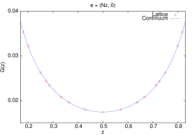
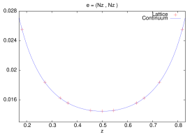
Figure 1: We show, for electric flux $\vec{e}=(Nz,0)$ (left), and $\vec{e}=(Nz,Nz)$ (right), the function $G(z)$ that gives the one-loop correction to the energy of a one-gluon state, through Eq. 134. The blue line corresponds to the continuum expression Eq. 135, while the red points are derived using a lattice regularization in the calculation of the self-energy.

The final result is quite compact and has many interesting properties that we want to comment about. The first important point is that the correction does not depend on the value of but only on the electric flux. Thus, the minimum energy within each sector corresponds to the minimum momentum $\rm{}_{\rm min}=\frac{2\pi\vec{n}}{NL}$. We will write it as follows:

$${{\cal E}^{2}(\vec{e})\over\lambda^{2}}={|\vec{n}|^{2}\over 4x^{2}}-{1\over x}\,G\Big{(}{\vec{e}\over N}\Big{)}\quad,$$ (134)

where we have introduced the variable $4\pi x=\lambda NL$, and the function:

$$G({\vec{z}})=-{1\over 16\pi^{2}}\int_{0}^{\infty}{dt\over\sqrt{t}}\,\Big{(}\theta_{3}^{2}(0,it)-\theta_{3}(z_{1},it)\,\theta_{3}(z_{2},it)-{1\over t}\Big{)}\quad.$$ (135)

This is a natural way to write it, since in 2+1 dimensions $\lambda$ has dimensions of energy, and appears as the natural unit. The three terms in Eq. 134 and $x$ are all dimensionless. Since the first term appearing in the dispersion relation is just the momentum squared, it is natural to interpret the correction as the mass squared. However, it is negative, since $G(\vec{z})$ is positive. As an illustration, we display in Fig. 1 the $\vec{z}=\vec{e}/N$ dependence of $G(\vec{z})$ for two different cases: $\vec{z}=(z,0)$, and $\vec{z}=(z,z)$. Notice that it peaks at $e/N$ close to $0$ and $1$. This feature is very relevant and will be commented about later. The red crosses in the figure result from a calculation of the self-energy correction using the lattice regularization that will be presented below. It agrees amazingly well with the continuum determination.

3.2.2 The Euclidean self-energy for the Wilson lattice regularization

Finally, in this subsection, we will present the calculation of the one-loop Eucliden self-energy using a lattice regularization. For the derivation we will make use of the results for the four dimensional case, with non-trivial twist on a two-torus, that have been obtained previously in [44]-[48]. Without much effort they can be translated into the three dimensional set up that we are facing here. For the sake of completeness, the generalization to 3 dimensions of the vacuum polarization derived in [44], [45] will be reproduced in Appendix B.

The starting point is a 3-dimensional lattice with $N_{s}$ sites in the spatial direction and infinite number of points in time. We will consider a discretization of the continuum action based on the Wilson plaquette action:

$$S_{W}=Nb\sum_{n\in{\bf Z}^{3}}\sum_{\mu\neq\nu}\Big{(}N-{\rm Tr}P_{\mu\nu}(n)\Big{)}\quad,$$ (136)

where $b=1/(\lambda_{L}a)$, with $a$ the lattice spacing and $\lambda_{L}$ ’t Hooft coupling on the lattice. $P_{\mu\nu}(n)$ represents the plaquette, written in terms of the SU($N$) link matrices $U_{\mu}(n)$ as:

$$P_{\mu\nu}(n)=U_{\mu}(n)U_{\nu}(n+e_{\mu})U_{\mu}^{\dagger}(n+e_{\nu})U_{\nu}^{\dagger}(n)$$

In the twisted box that we are considering, the spatial links satisfy the boundary conditions

$$U_{i}(n+N_{s}\hat{e}_{j})=\Omega_{j}(n)U_{i}(n)\Omega_{j}^{\dagger}(n+\hat{e}_{i})\quad.$$ (137)

The continuum limit is taken by sending $N_{s}\rightarrow\infty$ and the lattice spacing $a\rightarrow 0$, while keeping $L=aN_{s}$ constant. Note that in the Hamiltonian set up we are dealing with, the number of lattice points in the time direction is infinite and the momentum is hence cut-off at an UV scale $\pi/a$ for both spatial and temporal components. From now on and for simplicity we will set $a=1$.

For the Wilson lattice action, we can repeat the arguments used in the continuum and derive the lattice dispersion relation by imposing that the inverse lattice propagator, projected over transverse components, vanishes for lattice momentum $p=(i{\cal E}_{L},\rm)$. This gives:

$$\sinh^{2}({\cal E}_{L}/2)=\sum_{i}\sin^{2}(p_{i}/2)-{1\over 4}\sum_{\mu\nu}\varepsilon_{\mu}\Pi_{\mu\nu}^{L}(\rm)\varepsilon_{\nu}^{*}\Big{|}_{\rm on-shell}\quad,$$ (138)

where, at lowest order in $\lambda$, the lattice on-shell condition amounts to $p_{0}=i{\cal E}^{0}_{L}$, with:

$$\sinh^{2}({\cal E}^{0}_{L}/2)=\sum_{i}\sin^{2}(p_{i}/2)\quad.$$ (139)

The correction to the gluon energy in the continuum can be derived by evaluating ${\cal E}_{L}$ numerically, using the expressions for the lattice vacuum polarization presented in Appendix C, and extrapolating the results to the continuum limit by taking $N_{s}\rightarrow\infty$.

Here we will present a slightly modified version of the lattice dispersion relation that differs from the one above in the corrections at order $a^{2}$. The reason to do that is that the corresponding analytic formulas simplify considerably. For that, we will make use of the continuum expression on the right hand-side of Eq. 117 to approximate the lattice dispersion relation by:

$${\cal E}_{L}^{2}(\rm)\equiv 4\sum_{i}\sin^{2}(p_{i}/2)-\sum_{\mu}\Pi_{\mu\mu}^{L}(\rm)\Big{|}_{\rm on-shell}\quad.$$ (140)

Using the formulas for the vacuum polarization presented in Appendix C, one can easily derive the following expression at leading order in $\lambda_{L}$:

$$\delta{\cal E}_{L}^{2}(\rm)\equiv-\sum_{\mu}\Pi_{\mu\mu}^{L}\Big{|}_{\rm on-shell}(\rm)=$$ (141)

$$= {\lambda_{L}\over 4}+{g^{2}_{L}{\cal N}^{2}\over 6}\int_{-{\pi}}^{{\pi}}{dq_{0}\over 2\pi}\sum_{\vec{q}}^{\prime}\sum_{\mu}{F^{2}(\rm,\vec{q},-\rm-\vec{q})\over\widehat{q}^{2}}\Big{(}\widehat{q}_{\mu}^{2}+{3\widehat{(p+2q)}_{\mu}^{2}-6\tilde{V}^{(3)}_{\mu}\over 2\widehat{(p+q)}^{2}}-2\tilde{V}^{(4)}_{\mu}\Big{)}\Big{|}_{\rm on-shell}$$

$$- {g^{2}_{L}{\cal N}^{2}\over 4}\int_{-{\pi}}^{{\pi}}{dq_{0}\over 2\pi}\sum_{\vec{q}}^{\prime}\sum_{\mu}\Big{(}{1\over 2N}-{F^{2}(\rm,\vec{q},-\rm-\vec{q})\over 6}\Big{)}\Big{(}{\widehat{q}_{\mu}^{2}\widehat{p}_{\mu}^{2}\over\widehat{q}^{2}}\Big{)}\Big{|}_{\rm on-shell}\quad,$$

with

$$\tilde{V}^{(3)}_{\mu} = \cos^{2}\Big{(}{(p+q)_{\mu}\over 2}\Big{)}\widehat{(q-p)}^{2}+\cos^{2}\Big{(}{q_{\mu}\over 2}\Big{)}\widehat{(2p+q)}^{2}+\sum_{\rho}\cos^{2}\Big{(}{p_{\rho}\over 2}\Big{)}\widehat{(2q+p)}_{\mu}^{2}$$ (142)

$$+ 2\ \cos\Big{(}{(p+q)_{\mu}\over 2}\Big{)}\cos\Big{(}{q_{\mu}\over 2}\Big{)}\widehat{(q-p)}_{\mu}\widehat{(2p+q)}_{\mu}$$

$$- 2\ \cos\Big{(}{(p+q)_{\mu}\over 2}\Big{)}\cos\Big{(}{p_{\mu}\over 2}\Big{)}\widehat{(2q+p)}_{\mu}\widehat{(q-p)}_{\mu}$$

$$- 2\ \cos\Big{(}{p_{\mu}\over 2}\Big{)}\cos\Big{(}{q_{\mu}\over 2}\Big{)}\widehat{(2q+p)}_{\mu}\widehat{(2p+q)}_{\mu}\quad,$$

and

$$\tilde{V}^{(4)}_{\mu} = {1\over 4}\widehat{(q+p)}^{2}+3\cos^{2}\Big{(}{(q-p)_{\mu}\over 2}\Big{)}-3\cos({q_{\mu}})\sum_{\rho}\cos({p_{\rho}})$$ (143)

$$+ {1\over 3}\cos\Big{(}{q_{\mu}\over 2}\Big{)}\Big{\{}\widehat{p}_{\mu}\widehat{(q-p)}_{\mu}-2\ \widehat{p}_{\mu}\widehat{(q+p)}_{\mu}-\widehat{q}_{\mu}\widehat{(2p)}_{\mu}\Big{\}}$$

$$- {1\over 3}\cos\Big{(}{p_{\mu}\over 2}\Big{)}\Big{\{}\widehat{q}_{\mu}\widehat{(q-p)}_{\mu}+2\ \widehat{q}_{\mu}\widehat{(q+p)}_{\mu}+\widehat{p}_{\mu}\widehat{(2q)}_{\mu}\Big{\}}\quad.$$

Here, $\widehat{q}_{\mu}=2\sin(q_{\mu}/2)$, with $q_{i}=2\pi n_{i}/NN_{s}$, for $n_{i}=0,\cdots,N_{s}N-1$, and where the sum over $\vec{q}$ excludes momenta with $n_{i}=0$ (mod $N)\forall i$. Note that in the lattice formulation the linear divergences that arise in the different contributions to the self-energy cancel away in the sum and the final expression is UV finite.

To evaluate Eq. (141) numerically several steps are in order. We first fix the number of colours $N$ and the value of $\bar{k}$. Then, keeping the number of spatial sites ($N_{s}$) fixed, we evaluate the integrals over $q_{0}$ by discretizing the momenta in units of $2\pi/N_{0}$. Following Ref. [48], we improve the convergence of the finite sum over $q_{0}$ by shifting the pole of the propagator through the change of variables:

$$q_{0}\rightarrow q_{0}-{1\over 2}p_{0}-\gamma\sin(q_{0})\quad,$$

with $0\leq\gamma<1$, and $\gamma$ tuned close to 1 to improve the convergence of the sum. For fixed value of $N_{s}$, we increase $N_{0}$ until a stable result within machine precision is obtained for $G_{L}\equiv-x_{L}\,\delta{\cal E}_{L}^{2}/\lambda_{L}^{2}$, where $4\pi x_{L}=\lambda_{L}NN_{s}$. We generate in this way a set of values of $G_{L}$ for varying $N_{s}$ and extrapolate the results to $N_{s}\rightarrow\infty$. The extrapolation is obtained from a fit of the form:

$$G_{L}\Big{(}{e\over N}\Big{)}=G\Big{(}{e\over N}\Big{)}+\Big{(}b_{1}-b_{2}\ln(NN_{s})\Big{)}{1\over N^{2}N_{s}^{2}}+\Big{(}c_{1}-c_{2}\ln(NN_{s})\Big{)}{1\over N^{4}N_{s}^{4}}\quad.$$

As mentioned in the previous section, the continuum-extrapolated results obtained through this procedure match perfectly well the ones obtained in the continuum with dimensional regularization. This is exemplified in Fig. 1 for two values of the external momenta. The lines represent the continuum results, while the crosses indicate the results derived on the lattice.

3.3 General comments about the perturbative results and reduction

In the previous subsections we have analysed the perturbative calculation of the spectrum in our twisted box context. It is interesting to explore the general properties of this expansion. In particular let us focus on the dependence of our results on $N$ and $L$. It is clear that in momentum sums the two quantities enter in the combination $NL$. There is a slight correction due to the restriction induced by SU(N), since there is no component associated to vanishing colour momentum. The modification is termed slight since it affects only 1 of the $N^{2}$ degrees of freedom of the U(N) group. Now let us analyze the presence of $N$ and $L$ factors in the vertices. It is not hard to see that all vertices are proportional to the factor $g{\cal N}F$. Replacing the expressions given in the text we get: $-\frac{\sqrt{2\lambda}}{LN}\sin(\theta{\cal A})$. Notice that, once more, $L$ and $N$ appear combined as a product, once we express the formula in terms of ‘t Hooft coupling. The argument of the sine function is the area of the triangle formed by momenta meeting at a vertex, multiplied by the parameter $\theta$ appearing in Eq. 22. The parameter can be rewritten (for the square box case) as

$$\theta=\tilde{\theta}\times\Big{(}\frac{NL}{2\pi}\Big{)}^{2}\quad,$$ (144)

with $\tilde{\theta}$ given by Eq. 113.

Thus, we conclude that, according to perturbation theory, all physical results will depend on $\tilde{\theta}$, $\lambda$ and $LN$. Therefore, if we keep $\tilde{\theta}$ fixed, these results will depend jointly on $LN$. This is a form of volume independence or reduction, since finite volume effects would disappear, provided there is a well-defined large $N$ limit. On the other hand, if we achieve this limit with the alternative interpretation, L large and N fixed, we expect that the spectrum of the sector with vanishing electric flux should become independent of $\tilde{\theta}$. The reason is that this angle only affects the boundary conditions, and these should become irrelevant in the large volume limit. This argument does not apply for the non-zero electric flux sectors, because their masses continue to depend strongly on the size as we take it to infinity.

Another important point mentioned earlier, is that all energy scales could be expressed in units of $\lambda$. Because of dimensional counting, the ratio would appear as a power series expansion in the dimensionless quantity $\lambda L$. Combining this with our previous remarks, we conclude that the relevant expansion parameter would be

$$x=\frac{\lambda NL}{4\pi}$$ (145)

as was used previously in relation with the self-energy expression.

Thus, our final conclusion based on perturbation theory alone is that, as we take $N$ to infinity keeping $\tilde{\theta}$ fixed, we should recover the infinite volume limit. There are two provisos in this result. The first is that non-perturbative effects might not work the same way. We had indications of that in the study of the sphaleron solutions. This makes it very important to study the theory non-perturbatively to see what the behaviour really is. A first step in that direction will be presented in the next section. The other comment is that it becomes rigorously impossible to keep $\tilde{\theta}$ fixed as we change $N$. This is so because $\bar{k}/N$ is an irreducible rational number. To make the statement precise we have to assume that the final result would depend continuously on $\tilde{\theta}$. As $N$ grows, one could choose a sequence of values of $\bar{k}$ approximating $\tilde{\theta}$. In the next section we will see some examples.

Before, let us go back to the analysis of the consequences of our perturbative calculation of the minimum energy of the electric flux sectors. The formula (Eq. 134) reproduced below

$${{\cal E}^{2}(\vec{e})\over\lambda^{2}}={|\vec{n}|^{2}\over 4x^{2}}-{1\over x}\,G\Big{(}{\vec{e}\over N}\Big{)}\quad,$$ (146)

complies to the general pattern mentioned earlier. We remind the reader that $\vec{n}$ is given by the minimum momentum associated to a particular value of the electric flux

$$-\frac{N}{2}<(n_{i}=-k\,\epsilon_{ij}e_{j}\,(\bmod N))<\frac{N}{2}\quad.$$ (147)

As mentioned previously, the correction $\delta{\cal E}^{2}$ to the energy square could be considered the mass-square of the state. This interpretation seems bizarre since the quantity is negative. A particle with negative mass square is usually called a tachyon. A corresponding negative energy square would signal an instability. The state would be unstable and decay with a rate proportional to the imaginary part of the energy. The phenomenon is, thus, appropriately described as a tachyonic instability. Such a situation has been encountered in the context of field theories in non-commutative space-times [18, 20], where it was presented as signalling spontaneous breaking of $Z_{N}$ symmetry and electric flux condensation. Of course, as mentioned in the introduction, the question then is whether this tachyonic instability is present in our theory and, if so, what is its interpretation and the possible implications.

Of course, the negative mass-squared term does not necessarily imply any instability. At zeroth-order in perturbation theory our model has a mass gap, since the minimum momentum cannot vanish. Thus, for arbitrarily small coupling, the theory is stable. If we trust the one-loop result as exact, an instability would necessarily occur at

$$x_{T}(\vec{e})=\frac{|\vec{n}|^{2}}{4G(\frac{\vec{e}}{N})}$$ (148)

The point is then whether at this value of $x$ the perturbative formula remains valid or not. Notice that the reliability of this formula is higher, the smallest the value of $x_{T}$. Focusing on the values of $G$ displayed in Fig. 1 it might seem like a fairly large number. However, notice also that the function grows as $e/N$ approaches $0$ or $1$. This is not surprising because as $e/N$ approaches zero we should recover the UV divergence of the original integral. It is relatively simple to compute the behaviour close to the singularity by focusing on the integral producing the divergence

$$\int_{0}^{1}{dt\over t^{3/2}}\ \exp\Big{(}-{\pi|\vec{z}|^{2}\over t}\Big{)}=\,{1\over\ |\vec{z}|}+{\rm regular\ terms}\quad,$$ (149)

which leads to:

$${{\cal E}^{2}(\vec{e})\over\lambda^{2}}={|\vec{n}|^{2}\over 4x^{2}}-{N\over 16\pi^{2}x\,|\vec{e}|}\quad,$$ (150)

valid for $|\vec{e}|$ small enough. Plugging this result in the formula for the threshold for tachyonic behaviour we get

$$x_{T}={4\pi^{2}|\vec{e}||\vec{n}|^{2}\over N}\quad.$$ (151)

Taking $|\vec{e}|$ and $|\vec{n}|$ of order 1 and $N$ going to infinity, seems to lead unavoidably to a tachyonic instability setting in at $x=x_{T}$.

However, $|\vec{e}|$ and $|\vec{n}|$ are not unrelated quantities. If we forget about the modulo $N$ part and simply replace $n_{i}=-k\epsilon_{ij}e_{j}$ in the previous formula we get

$$x_{T}={4\pi^{2}|\vec{e}|^{3}k^{2}\over N}\quad.$$ (152)

where $k$ is the magnetic flux. If we scale the magnetic flux like $N$ (or even $\sqrt{N}$) in the large N limit, we keep the tachyonic threshold $x_{T}$ safely away from the perturbative region. On the opposite extreme if we take the lowest momentum value $n=1$, this corresponds to an electric flux of $\bar{k}$. Hence, to avoid instabilities we should take the large N limit keeping $\bar{k}/N$ bounded from below. It is remarkable that our criteria correspond to similar ones advocated by González-Arroyo and Okawa [25] for large $N$ reduction to apply for the twisted Eguchi-Kawai model in 4-dimensions.

It is clear that our analysis has opened many questions about the region of validity of the perturbative regime and its consequences that only a non-perturbative analysis can settle. This is indeed the purpose of the numerical results that will be presented in section 4.

4 Non-perturbative lattice determination of the mass spectra

4.1 The goals

In the previous section we have studied, by perturbative techniques, the behaviour of 2+1 SU(N) Yang-Mills fields defined on a finite spatial torus with twisted boundary conditions. Several interesting properties emerged concerning the $N$ and $L$ dependence of physical observables. In particular, we observed that with appropriate choices of the magnetic flux through the box, physical observables depend jointly on the product $NL$, or rather on the dimensionless quantity $x=\lambda NL/(4\pi)$. We also observed that, in certain circumstances, perturbation theory suggested the appearance of tachyonic instabilities. Both phenomena are well exemplified by the formula for the ground state energies in the sectors of non-zero electric flux $\vec{e}$ (Eq. 134), valid for small values of $x$. The purpose of this section is to explore the evolution of these quantities for larger values of $x$. This will allow us to determine the region of validity of the perturbative formulas and to test if and when tachyonic instabilities will appear. Last, but not least, we can check whether $NL$ scaling continues to hold in the non-perturbative region.

In order to justify our particular setting, it is necessary to be more specific about what quantities will be explored and why. Since we want to follow the transition from the perturbative to the non-perturbative region, we have concentrated on those quantities which are easier to track in both regimes. Thus, we will focus on straight line Polyakov loops having the minimal and next to minimal momentum values $\rm=(\frac{2n\pi}{NL},0)$ (with $n=1,2$) (we disregard here the mixed momenta $\rm=\frac{2n\pi}{NL}(\pm 1,\pm 1)$ which have lower perturbative energy than the $n=2$ states). To simplify notation, in what follows, we will refer to these quantities as ${\cal E}_{1}$ and ${\cal E}_{2}$ for the $n=1$ and $2$ cases respectively. The $n=1$ loops are the lowest excited states over the vacuum in the perturbative regime. As we will see, this will not be the case in general for the large $x$ region. We should emphasize that, even if we stick to these momenta, one still covers a wide range of electric flux values by changing the magnetic flux of the box. We recall that the relation between the integer $n$ appearing in the momentum formula and electric flux is $|\vec{e}|=\bar{k}n\bmod N$, where $\bar{k}k=1\bmod N$. Notice that, with twisted boundary conditions, there are no zero-momentum states carrying electric flux.

Concerning the behaviour of these quantities in the perturbative region it is interesting to make a few observations. While at zero order in perturbation the minimum $n=1$ momentum contains a unique state having the lowest energy (indeed the first excited state over the vacuum), for the $n=2$ case there are actually two degenerate states corresponding to one gluon or two collinear gluons. Since these states have the same quantum numbers they can mix. To order $\lambda$ the degeneracy is broken by the self-energy term, but mixing remains absent. Which of the two states is lighter, follows by comparing $G(2\bar{k}/N)$ with $4G(\bar{k}/N)$, and the answer depends on the value of $\bar{k}$.

In order to interpret our results it is interesting to revise what is the expected behaviour of our observables for large torus sizes. Confinement dictates that all states carrying non-vanishing electric flux should have energies that grow linearly with the size of the box $L$. A priori, one expects that the energy per unit length –the string tension– should depend only on the value of the electric flux and neither on the particular momentum chosen $n$, nor on the magnetic flux through the torus $k$:

$${{\cal E}_{n}\over\lambda}={\sigma_{\vec{e}}\,L\over\lambda}\quad.$$ (153)

The dependence of the string tension $\sigma_{\vec{e}}$ on the electric flux $\vec{e}=(0,e)$ is a very interesting property, around which considerable literature has been generated. The expected dependence is as follows:

$$\sigma_{e}=N\sigma^{\prime}\,\phi\Big{(}{e\over N}\Big{)}\quad,$$ (154)

where $\sigma^{\prime}$ can be fixed in terms of the ordinary string tension, which corresponds to one unit of electric flux. The function $\phi(z)$ should behave as $z$ for small argument, and by definition should satisfy $\phi(z)=\phi(1-z)$. There are two forms of $\phi(z)$ which have appeared repeatedly in the literature when studying various theories, either exactly or with approximations:

$$\phi(z)=z(1-z)$$

and

$$\phi(z)=\sin(\pi z)/\pi\quad.$$

We point out that the k-string formula Eq. 154 is in perfect agreement with our $x$ scaling hypothesis, since the linear behaviour of the energies can be rewritten as

$${{\cal E}_{n}\over\lambda}=4\pi x\frac{\sigma^{\prime}}{\lambda^{2}}\,\phi\Big{(}{e\over N}\Big{)}\quad.$$ (155)

We remind the reader that the $x$-dependence holds for fixed values of $\bar{k}/N$. For $n=1$, $e$ and $\bar{k}$ are just equal, while for $n=2$, $e=2\bar{k}\bmod N$.

The way in which the linear regime is approached, as $L$ grows from small to large values, has also been studied intensively for various confining theories, including 2+1 dimensional gauge theories. The picture that the fluctuating flux tubes can be described by an effective string theory has received strong support by recent lattice studies. For example, the work of Ref. [51] showed an spectacular agreement with the spectrum of the Nambu-Goto string. This goes beyond the behaviour having an universal character (irrespective of the particular string theory involved). In this respect, for the three-dimensional theory, it has been shown [52] that the first two coefficients in the expansion of the string energy in powers of $1/(\sigma L^{2})$ are universal.

This predicted $L$ dependence is very important in order to interpret our results. However, we might question how these conclusions are affected by our particular twisted box setting. Previous studies concerned the case of only one compact direction rather than two. Furthermore, one might wonder what effect does the presence of the twist have upon the string description. As a matter of fact, our work might help in giving support to a particular scenario of this type. There are remarkable indications that twisted boundary conditions could be related with string models on the background of Kalb-Ramond $B$-fields. We will explain below why this is indeed the most natural choice. The Nambu-Goto prediction for the energy of a closed-string winding $\vec{e}$ times around a torus on the background of a Kalb-Ramond $B$-field, is derived from:

$${{\cal E}^{2}(\vec{e})\over\lambda^{2}}=\Big{(}{\sigma|\vec{e}|L\over\lambda}\Big{)}^{2}-{\pi\sigma\over 3\lambda^{2}}+\sum_{i}\Big{(}{\epsilon_{ij}e_{j}\,B\over\lambda L}\Big{)}^{2}\quad,$$ (156)

The $B$-dependent term in this expression has an intriguing analogy with the pertubative expansion for the electric-flux energy. It suffices to recall that $\epsilon_{ij}e_{j}=-\bar{k}n_{i}({\rm mod}N)$, with $\rm=2\pi\vec{n}/NL$ the gluon momentum, to suggest the identification: $B\equiv-2\pi k/N$. This transforms the $B$-field dependent term into the tree-level perturbative contribution: $|\vec{n}|^{2}/(4x^{2})$.

On second thoughts, the connection between twisted boundary conditions and strings with Kalb-Ramond $B$-fields is also suggested by their common relation to non-commutative quantum field theory. In the open string sector, the latter appears as a particular low-energy limit of these type of string theories [50], with non-commutativity parameter $\theta_{ij}\equiv-\epsilon_{ij}L^{2}/B$. Combining this with the expression given above for the $B$-field readily reproduces the field-theory $\theta$ parameter introduced for the twisted box in Eq. 22.

This observation allows to cast the spectrum of the closed Nambu-Goto string on the background of a $B$-field into a form fully consistent with the conjectured $x$ dependence of all physical observables:

$${{\cal E}^{2}(\vec{e})\over\lambda^{2}}=\Big{(}{4\pi\sigma|\vec{e}|\over N\lambda^{2}}\Big{)}^{2}x^{2}-{\pi\sigma\over 3\lambda^{2}}+{|\vec{n}|^{2}\over 4x^{2}}\quad,$$ (157)

connecting, in a very remarkable way, perturbation theory in the twisted box with the Nambu-Goto string dynamics. From this formula we deduce that the first two terms are not affected by the presence of the twisted boundary conditions, which will allow us to make use of the results obtained in other settings.

4.2 The methodology

Having fixed our goals, we will now describe the way in which we have set up our methodology to accomplish them. We will be using lattice gauge theory techniques, which have proved to be a powerful tool to investigate non-perturbative phenomena in gauge theories. More detailed aspects of our technique follow.

Twisted boundary conditions can be very easily implemented on the lattice. The starting point is the Wilson lattice action given in Eq. 136 with link matrices satisfying the boundary conditions specified in Eq. 137. It is possible to perform a change of variables that allows one to work with periodic links at the price of introducing a twist dependent factor in the action. The new action reads

$$S_{W}=Nb\sum_{n\in{\bf Z}^{3}}\sum_{\mu\neq\nu}\Big{(}N-z_{\mu\nu}^{*}(n){\rm Tr}P_{\mu\nu}(n)\Big{)}\quad,$$ (158)

where $z_{\mu\nu}(n)$ is equal to 1 except for the corner plaquettes in each (1,2) plane where it takes the value:

$$z_{ij}(n)=\exp\Big{(}i\epsilon_{ij}{2\pi k\over N}\Big{)}\quad.$$ (159)

In order to explore the volume and $N$ dependence as a function of the magnetic flux, we have performed a set of Monte Carlo simulations for various values of $k$, the gauge group SU($N$), the lattice size $N_{s}=L/a$, and $b\equiv 1/(a\lambda_{L})$, where $a$ is the lattice spacing and $\lambda_{L}$ is ‘t Hooft coupling on the lattice. The temporal extent, with $N_{0}$ sites, has been chosen sufficiently large to avoid significant finite temperature effects. Our simulations allow us to cover a wide range of values of $x_{L}=NN_{s}/(4\pi b)$, which is the lattice counterpart of the dimensionless quantity $x$ introduced earlier. Similarly, multiplying $b$ by the spectrum as measured on the lattice we get $b\,{\cal E}_{L}$, the lattice equivalent to the ratios ${\cal E}/\lambda$. Lattice counterparts differ from the continuum values by a function of $a\lambda$ which goes to zero as $a\lambda\sim 1/b$ goes to zero. Thus, to recover the continuum results one should take $b$ and $N_{s}$ to infinity with a fixed ratio. For the exploratory study, contained in this paper, we will be moderately ambitious and work at a few fixed values of $N_{s}$ and $N$ but range over many values of $b$, which will allow us to scan a wide set of values of $x_{L}$, ranging from the perturbative regime to the domain where confinement of electric fluxes sets in. Notice, however, that in this way the lattice corrections would affect mostly the results obtained for larger values of $x_{L}$.

Our choice of values of $N$ and $N_{s}$ was designed to test the validity of our conjecture that physical results will depend only on the product $NL$. With this purpose in mind, we have analyzed four sets of $(N,N_{s},N_{0})$ values: (5,22,72), (5,14,48), (7,10,32), and (17,4,32), with magnetic fluxes: $k=1,2$ for SU(5), $k=1,2,3$ for SU(7), and $k=1,3,5,8$ for SU(17). The last three sets have been chosen to have approximately equal values of $NN_{s}$. The first, with the same value of $N$ as the second but larger $N_{s}$, was included as a measure of the effects of lattice artifacts. The results obtained at the same value of $x_{L}$ for the first set should be closer to the continuum.

As mentioned previously, our analysis will be focused on the electric-flux states generated by straight Polyakov lines that have minimal and next to minimal momentum values $\rm=(\frac{2n\pi}{NL},0)$ (with $n=1,2$). We have considered two different lattice operators projecting onto these states. They are represented by the product of link matrices:

$${\cal P}(t,x;w)={\rm Tr}\Big{\{}\prod_{s=0}^{N_{s}-1}U_{2}(t,y+s,x)\Big{\}}^{w}\quad,$$ (160)

with the two possible choices given by $w=-n\bar{k}\,(\bmod N)$ and $w=N-n\bar{k}\,(\bmod N)$. The spectrum has been extracted from correlators of these operators projected over the appropriate momenta through:

$$C_{n}(t;w)={1\over N_{s}}\sum_{x,\tilde{x}}\exp\Big{(}-i2\pi\,{n\tilde{x}\over N_{s}N}\Big{)}\,\langle{\cal P}(0,x;w){\cal P}^{\dagger}(t,x+\tilde{x};w)\rangle\quad.$$ (161)

The ground state mass within each electric-flux sector can be determined as usual from the late time decay of the correlator. Of the two operators indicated above, we have used in each case the one that shows less contamination of excited states and gives a lowest ground-state mass.

For the type of correlators that were studied in this work we could obtain good results by using smeared Polyakov loops. Hence, it has not been necessary to implement other state of the art techniques designed to improve the projection onto the ground state. This is exemplified in Fig. 2, where we show several characteristic effective mass plots, corresponding to both the perturbative and the confining regimes. Before continuing, let us point out that the smearing procedure has to be slightly modified in the twisted box by introducing the twist tensor, $z_{ji}$, in the definition of the staples. With this, smearing proceeds as usual by iteratively replacing the spatial link matrices by:

$$U_{i}^{(s+1)}(n)=(1-c)\,U_{i}^{(s)}(n)+{c\over 2}\sum_{\pm j,j\neq i}\!z_{ji}\,U_{j}^{(s)}(n)U_{i}^{(s)}(n+j)U_{j}^{(s)\dagger}(n+i)\Big{|}_{\rm unitarized}\quad.$$ (162)

The results that will be presented below were obtained with smearing parameter $c=0.475$ and 20 smearing steps.

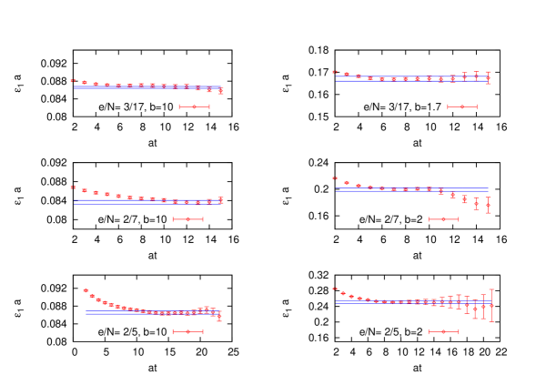
Figure 2: We show several characteristic effective mass plots for ${\cal E}_{1}$, the energy of electric flux $|\vec{e}|=\bar{k}$ with momentum $|\rm|=2\pi/NL$. They correspond to the perturbative (Left) and the confining (Right) regimes.

Finally, let us briefly describe the details of the algorithm employed in the Monte Carlo simulations. It is well know that the standard Creutz’s heat bath-algorithm has a very low acceptance rate both at weak coupling and for SU(N) gauge theories at large $N$. To prevent this, we have used instead a heat-bath algorithm based on a proposal by Fabricius and Haan [49] that significantly improves the performance in these two cases. In Creutz’s method, one sweeps through all possible SU(2) subgroups of SU(N) with probability given by:

$$\,{\rm d}\alpha_{0}\,\sqrt{1-\alpha_{0}^{2}}\ \exp(4bNk\alpha_{0})\quad.$$ (163)

For large $b$ and(or) large $N$, the exponential factor nearly always gives $\alpha_{0}\approx 1$, which is most of the times rejected with probability $\sqrt{1-\alpha_{0}^{2}}$. To circumvent this, Fabricius and Haan introduced the variable $\alpha_{0}=1-2\delta^{2}$, with probability distribution

$$\,{\rm d}\delta\,\delta^{2}\,\sqrt{1-\delta^{2}}\ {\rm exp}(-8bNk\delta^{2})\quad.$$ (164)

By introducing a three-dimensional vector $\vec{\delta}$, this becomes

$$\,{\rm d}^{3}\vec{\delta}\,\sqrt{1-|\vec{\delta}|^{2}}\ {\rm exp}(-8bNk|\vec{\delta}|^{2})\quad.$$ (165)

Then the exponential factor nearly always gives $|\vec{\delta}|\approx 0$ for large $\beta$ and(or) large $N$, which is accepted with $\sqrt{1-|\vec{\delta}|^{2}}$ probability. With this method at hand, one of our Monte Carlo sweeps consists of the heat-bath updating of all possible SU(2) subgroups of SU(N), followed by 5 over-relaxation updatings.

A compilation of all our numerical results is presented in the tables of Appendix D. For each data set, a characteristic ensemble consists on $1-2\times 10^{6}$ Monte-Carlo sweeps with all the observables measured every 40 sweeps. Both the errors on the correlators as those on the fitted masses have been determined using jackknife. Let us finish by mentioning that the characteristic run-times for the $SU(17)$ lattice, for instance, are 0.15 seconds/Monte-Carlo sweep, running on 16 cores of the IFT Hydra cluster (specifications can be found at http://www.ift.uam-csic.es/hydra/).

4.3 Analysis of Numerical Results

In this subsection we will present the numerical results obtained with the lattice regularization. As explained before, we have restricted our analysis to the evaluation of the temporal correlation function of straight Polyakov lines with minimal $\rm=(\frac{2\pi}{NL},0)$ and next-to-minimal momentum $\rm=(\frac{4\pi}{NL},0)$. The corresponding energies will be labelled ${\cal E}_{1}$ and ${\cal E}_{2}$ respectively. The bare results have been collected in tables in appendix D. This will allow other researchers to use and analyse the data according to their criteria. In what follows we will present our particular analysis of the numerical data.

Let us focus first on the results for the minimum momentum, with energy ${\cal E}_{1}$. A visual representation of the results is given in Fig. 3, in which the combination $x{\cal E}_{1}/\lambda$ is displayed as a function of $x$. Each set of points is represented in different colours and labelled by the combination $\bar{k}/N$ characteristic of the data sample. They have been grouped into subplots which display different ranges of the ratio $\bar{k}/N$, increasing from left to right. The continuous lines are the results of a fit to be explained later but, at this level, they are very helpful to guide the eye. A simple look at the figure shows the similarity among the different curves despite the difference in the value of $N$ and of the magnetic fluxes used. The visual agreement is in accordance to our hypothesized universal $x$ behaviour at fixed value of $\tilde{\theta}=2\pi\bar{k}/N$. The differences observed could be explained by the fact that the values of $\bar{k}/N$ are not exactly equal for each set of data points. Indeed, the closest values occur for $N=7$ and $\bar{k}=2$ and $N=7$ and $\bar{k}=5$. The results of these two cases, appearing in the middle subplot, show a striking resemblance.

The general features of the figures also agree with the expectations described earlier. The lowest order perturbative result, valid for small $x$, gives $0.5$, which agrees with the data. The correction comes from the self-energy term computed in this paper and accounts for the decrease observed at small but higher values of $x$. The way in which we have represented the data allows a very clear recognition of the perturbative features. If we continue for larger values of $x$, we observe that the decrease reaches a minimum at around $x\sim 1$, and then grows very fast for larger $x$. The fact that the decrease ceases before the energy becomes negative is precisely what we anticipated. It shows that the perturbative formulas cannot be trusted in this case beyond values of order 1. Hence, no tachyonic instability occurs in any of these data sets. We have left out temporarily of the analysis those cases in which perturbation theory indicates the generation of tachyonic instabilities at small values of $x$. That cases will be studied in the next subsection.

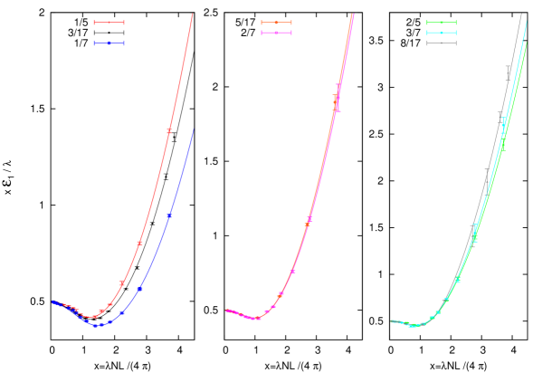
Figure 3: We display $x{\cal E}_{1}/\lambda$ as a function of $x$. The lines are fits derived from Eq. (168) with parameters set as discussed in section 4.3. The labels in the plot indicate the value of $\bar{k}/N$.

Finally, we should mention that the rise of the curves at large $x$ is simply what confinement predicts. To allow a more clear visual comparison of the results and the expectations, we have displayed in Fig. 4 the values of $({\cal E}_{1})^{2}/(\lambda x)^{2}$ after subtracting out $1/(4x^{4})$, which is the zero-order perturbative result for this quantity. The curves look very much consistent with the expectation that they should tend towards constant values at infinity with a $1/x^{2}$ pattern. The constant at infinity is nothing but the string tension. It is certainly not chance that the order of the curves corresponds neatly to the order of the values $e/N=\bar{k}/N$.

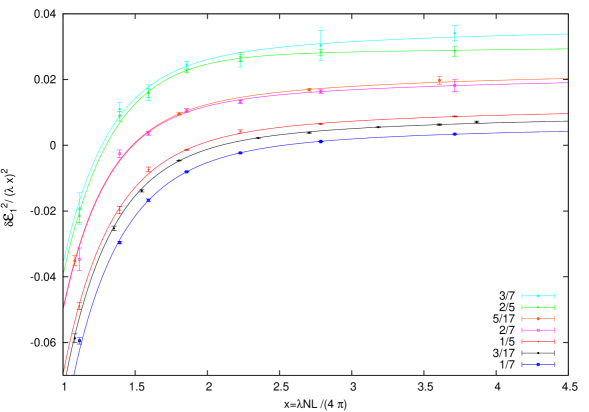
Figure 4: We display ${\cal E}_{1}^{2}/(\lambda x)^{2}$ after subtracting out $1/(4x^{4})$, which is the zero-order perturbative contribution to this quantity. The lines are fits derived from Eq. (168) with parameters determined as discussed in section 4.3. The labels in the plot indicate the value of $\bar{k}/N$.

$\bar{k}$	N	$G(\bar{k}/N)$	$\gamma$	${\cal A}$	$S_{0}$
1	5	0.0322615	0.110(2)	14(3)	7.5(4)
2	5	0.0185816	0.177(4)	27(8)	8.0(4)
1	7	0.0446267	0.081(1)	20(2)	8.1(2)
2	7	0.0234449	0.147(5)	12(6)	6.9(7)
3	7	0.0180238	0.190(7)	14(10)	7.2(1)
3	17	0.036346	0.099(2)	14(2)	7.4(3)
5	17	0.0228957	0.152(3)	10(3)	6.9(4)
8	17	0.0175579	0.210(5)	36(76)	10(3)

Table 1: We present the set of parameters corresponding to the fits used to describe the ${\cal E}_{1}$ data displayed in Figs. 3 and  4.

Thus, visual scrutiny shows that our anticipated results are not inconsistent with the data. It is necessary to go beyond this stage and attempt a more quantitative analysis of our results. For that purpose we have tried to describe the data with a parameterization inspired by the theoretical considerations presented at the beginning of this section. Collecting all the different contributions expected from the different sources, we are led to an expression of the type:

$${{\cal E}_{1}^{2}\over\lambda^{2}}={1\over 4x^{2}}+{\alpha\over x}+\beta+\gamma^{2}\,x^{2}\quad,$$ (166)

It follows both from the perturbative results and from the string fluctuation description, that it is advisable to parametrise ${\cal E}_{1}^{2}$ rather than ${\cal E}_{1}$. By construction this formula should describe well the behaviour of our data in the asymptotically small and large $x$ regimes. This is indeed the case. This simple ansatz describes also qualitatively well the transition region between both regimes shown by our data. Not satisfied with this result, we have aimed at having a quantitatively good description of the region of intermediate $x$ values. Curiously a simple additional term of the form

$$\frac{{\cal A}}{x^{a}}\,\exp\Big{\{}-{S_{0}\over x}\Big{\}}\quad,$$ (167)

allows us to achieve our goal. Although of a phenomenological nature, the form of the additional term was inspired by the posible presence of non-perturbative contributions around additional instanton-like configurations. The shape is the one arising from a semiclassical analysis. Indeed, this would not be completely unexpected. Monopole like contributions have been found to be crucial to achieve confinement in abelian gauge theories, and monopoles are just instanton-like in 2+1 dimensions. Furthermore, there are at least some non-perturbative 2-d configurations, studied in section 2, which look like sphalerons and appear as the top of the hill for a corresponding instanton configuration. Certainly, both the numerical study of the transition region, as well as the presence and dynamical contribution of semiclassical configurations, deserves further study. For the time being, we let the reader judge what relevance should be given to the fact that such a term allows us to describe the transition region with rather good precision.

The additional term adds three parameters, which are however too highly correlated to let our data determine them. After exploring different choices we found that fixing $a=7/2$ allows us to describe all the data.

In summary, the final parameterization used to fit the data in figures 3 - 4 is of the form:

$${{\cal E}_{1}^{2}\over\lambda^{2}}={1\over 4x^{2}}+{\alpha\over x}+{{\cal A}\over x^{3}\sqrt{x}}e^{-{S_{0}\over x}}+\beta+\gamma^{2}\,x^{2}\quad.$$ (168)

Before proceeding to present the results of the fits, let us discuss a bit more about the origin and possible values of the parameters. Our perturbative formulas account for the first and second terms of our expression, with $-\alpha$ replaced by the self-energy function $G(\vec{z})$, computed and displayed in section 3.2. Therefore, we fixed this parameter to this value in all our fits, after verifying that leaving this parameter free does not alter substantially the quality of the fit. One the other hand, the $\gamma$ and $\beta$ terms have the form following from a confining linear potential, corrected by universal subleading corrections arising in an effective string picture [52]. At leading order in $1/(\sigma L^{2})$, one expects: ${\cal E}/(\sigma L)=1+\pi\rho/(\sigma L^{2})$, where the second term is the universal Lüscher correction, with coefficient $\rho=-1/6$ for the fundamental closed string in three dimensions. An interesting question, relevant for the study of the $k$-string dynamics, is what is the dependence of this coefficient on the electric flux $e$ (see e.g. [3], [51], [53], [54]). Within our parameterization, $\rho=2\beta/(N\gamma)$. Thus, our results can provide interesting information in this respect.

After these considerations, we present the results of the fits. All data points corresponding to particular values of $N$ and $N_{s}=L/a$, are well fitted by our formula having four free parameters (${\cal A}$, $S_{0}$, $\beta$ and $\gamma$). From these results one can analyse the behaviour of $\rho$ as a function of the $e/N$ ratio. The results, displayed in Fig. 5, are consistent with a formula of the type:

$$N\rho(z)\equiv{2\beta\over\gamma}=-{{\cal C}\over z(1-z)}\quad,$$ (169)

with ${\cal C}=1/6$ in this case. Fixing this relation allows us to obtain equally good fits to the whole sample with less parameter correlations and, hence, reduced errors. This is just a three parameter fit which describes the data rather well. The continuum curves displayed in Figs. 3 and  4 are the result of these fits. The corresponding parameters are presented in Table 1.

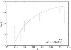
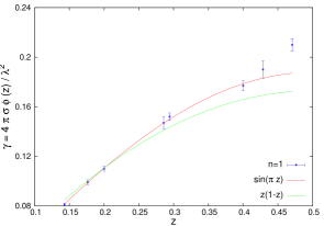
Figure 5: On the left plot we display the function $N\rho(z)$, given in Eq. 169, as a function of $z=e/N$. This quantity equals ($N$ times) the coefficient of the Lüscher term in the effective string expansion. On the right plot we display the function $\gamma(z)=4\pi\sigma^{\prime}\phi(z)/\lambda^{2}$, given in Eq. 170. The red line in the plot is a fit to the Sine scaling formula: $\phi(z)=\sin(\pi z)/\pi$. The green line corresponds to the prediction from Casimir scaling: $\phi(z)=z(1-z)$.

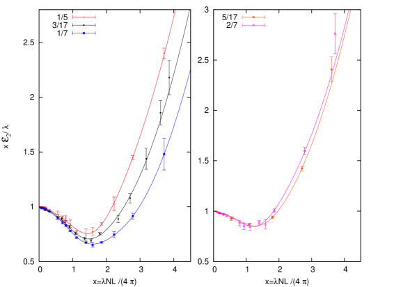
Figure 6: We display $x{\cal E}_{2}/\lambda$ as a function of $x$. The lines are fits derived from Eq. (168) with parameters determined as discussed in section 4.3. The labels in the plot indicate the value of $\bar{k}/N$.

Our results also allow us to extract relevant information on the values of the string tension for these states. Following the discussion around Eq. 154, we parameterize $\gamma$ as:

$$\gamma(z)={4\pi\sigma^{\prime}\over\lambda^{2}}\phi(z)\quad.$$ (170)

The information on what is the relevant scaling of the $k$-string tension with the electric flux is thus encoded in the function $\phi(z)$. In the right plot of Fig. 5 we display $\gamma(z)$ for our data set, which includes all the results for different gauge gauge groups and magnetic fluxes. The lines in the plot correspond to two of the most commonly discussed scaling functions for the $k$-string tension: Casimir scaling: $\phi(z)=z(1-z)$, and the Sine scaling: $\phi(z)=\sin(\pi z)/\pi$. Clearly the latter is in a much better accordance with the data giving a $\chi^{2}$ per degree of freedom of order 0.34 (if the point at largest value of $z$ is excluded). The value obtained from this fit for the large N fundamental string tension is $\sqrt{\sigma^{\prime}}/\lambda=0.217(1)$. It deviates around 10$\%$ from the large $N$ value obtained by Teper and collaborators in Ref. [3]: $\sqrt{\sigma}/\lambda=0.19638(9)$. Given the limitations of our numerical analysis, and the absence of a continuum extrapolation, this agreement can be considered very satisfactory.

Let us now briefly comment about the results of the $n=2$ momenta states. The quality of the data is poorer and we have to face additional complications, as the mixing of states occurring in pertubation theory. Hence, the results for $x{\cal E}_{2}/\lambda$ as a function of $x$, presented in Fig. 6, do not have the quality of the $n=1$ case. Notice that we have left out of the figure the set corresponding to the rightmost plot in Fig. 3, where perturbation theory indicates the existence of instabilities at this value of the momentum for small values of $x$. The corresponding data will be discussed in the next subsection.

The continuum curves in the plot correspond again to the parameterization of the energy given in Eq. 168. Here we had to deal with the complication introduced by the degeneracy at zero-order in perturbation theory between one gluon and two collinear gluon states. This degeneracy is broken by the self-energy contribution and accordingly we have taken $-\alpha={\rm max}\{G(2\bar{k}/N),4G(\bar{k}/N)\}$. For all the values of $\bar{k}/N$ displayed in the figure this consideration favours the second choice, and indeed its value is the one that appropriately describes our data. Concerning the parameters $\alpha$ and $\beta$, the precision in this case is not good enough to obtain a reliable independent determination of both. Nevertheless, if we fix $\gamma(z)$ according to Eq. 170, with $\phi(z)$ and $\sigma^{\prime}$ given by the Sine scaling formula, the resulting three parameter fit describes rather well the data. The corresponding parameters are presented in Table 2. The analysis of the Lüscher term based on these results is consistent with an scaling in $z=e/N$ given by the same equation 169 that describes the $n=1$ results, but with a coefficient ${\cal C}$ that is about four times larger.

$2\bar{k}$	N	$4G(\bar{k}/N)$	$G(2\bar{k}/N)$	$-\beta$	${\cal A}$	$S_{0}$
2	5	0.129046	0.0185816	0.231(23)	282(50)	10.6(6)
2	7	0.1785068	0.0234449	0.295(8)	118(7)	8.2(2)
3	7	0.0937796	0.0446267	0.219(25)	160(30)	8.8(5)
6	17	0.145384	0.0199961	0.294(13)	126(14)	8.5(3)
7	17	0.0915828	0.0183267	0.187(21)	111(31)	9.0(6)

Table 2: We present the set of parameters corresponding to the fits used to describe the ${\cal E}_{2}$ data displayed in Fig. 6.

4.4 Tachyonic instabilities

In this subsection we will address the possible occurrence in our results of tachyonic instabilities, as suggested by perturbation theory. We argued that, if the calculated threshold for instabilities $x_{T}$ does not turn out to be small, their presence has to be considered questionable. The data presented in the previous subsection verified that this is indeed the case: no instabilities occurred. On the contrary, if $x_{T}$ is small or very small, the perturbative indication of an instability should be considered seriously. Our perturbative discussion identified the cases of small of $\bar{k}/N$ and/or $k/N$ values as credible candidates for a tachyonic instability to set in. Within our data set there are two particular points that fall into this category. The first one corresponds to $n=1$, $N=17$ and $k=\bar{k}=1$, and the second to $n=2$, $N=17$ and $k=2$. In what follows, we will compare the expectations with the actual results for these cases.

In section 3.3 we gave as estimate for the threshold for instabilities $x_{T}=|\vec{n}|^{2}/(4G(e/N))$. By making use of our fitting function Eq. (168) we are now in condition for improving this estimate. This will allow us to test, beyond perturbation theory, the conditions leading to instabilities. For the energy to remain non tachyonic we should impose:

$${{\cal A}\over x\sqrt{x}}\,e^{-{S_{0}\over x}}+{|\vec{n}|^{2}\over 4}+\alpha\,x+\beta\,x^{2}+\gamma^{2}\,x^{4}\geq 0\quad.$$ (171)

Given that ${\cal A}\geq 0$, a simpler operational expression can be obtained by setting ${\cal A}=0$. In that limit, the energy is non-tachyonic whenever the quartic equation:

$${|\vec{n}|^{2}\over 4}+\alpha\,x+\beta\,x^{2}+\gamma^{2}\,x^{4}=0$$ (172)

does not have real roots. This is the case if and only if the discriminant is bigger than zero and the following condition, defined in terms of the Lüscher parameter $\rho$, is satisfied:

$${\cal H}\equiv{|\vec{n}|^{2}\over N^{2}}-{1\over 4}\,\rho^{2}(e)>0\quad.$$ (173)

It is interesting to point out that $-N^{2}{\cal H}$ is the discriminant of the equation obtained by setting the parameter $\alpha$ to zero in Eq. 172. In this limit we recover the Nambu-Goto string spectrum from Eq. 157. Hence, ${\cal H}>0$ is the bound to avoid tachyonic behaviour coming from the string component of the equation. The condition on the positivity of the discriminant for $\alpha\neq 0$ turns out to be a more restrictive one. After some algebraic manipulation it can be cast in the form:

$$4|\vec{n}|^{2}\,\gamma^{2}{\cal H}^{2}+4\beta\,{\alpha^{2}\over N^{2}}\,({\cal H}+8{|\vec{n}|^{2}\over N^{2}})-27\,{\alpha^{4}\over N^{4}}>0\quad,$$ (174)

Notice that, since $\beta<0$, the bound is violated for ${\cal H}=0$. The condition derived from the string formula is thus replaced by the more stringent one: ${\cal H}>{\cal H}_{0}$, with ${\cal H}_{0}$ the positive solution of the quadratic equation that saturates the bound. For small ${\cal H}_{0}$ we can still approximate the result by imposing ${\cal H}>0$. Parameterizing now the electric flux dependence of $\rho$ by $N\rho(z)=-{\cal C}/z(1-z)$, as in the previous subsection, we arrive at the following condition to prevent the appearance of tachyonic instabilities:

$$|\vec{n}|\,{|\vec{e}|\over N}\,\Big{(}1-{|\vec{e}|\over N}\Big{)}>\,{{\cal C}\over 2}\quad.$$ (175)

where the constant ${\cal C}$ is approximately $1/6$.

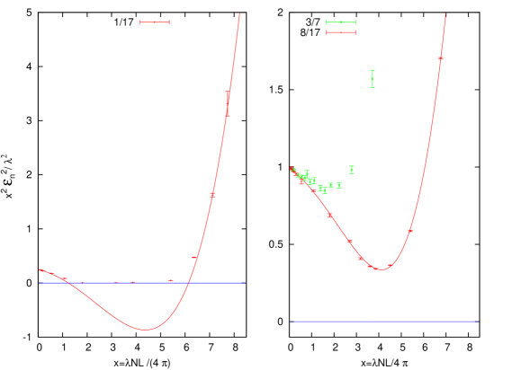
Figure 7: We display $x^{2}{\cal E}^{2}_{n}/\lambda^{2}$ vs $x$, in the sector of electric-flux $e=1$, for: Left: $n=1$, $\bar{k}=k=1$, and Right: $n=2$, $k=2$, $\bar{k}=(N-1)/2$. The continuum lines represent fits to the data derived from Eq. (168) with parameters fixed as described in section  4.3. For the fit in the left plot the condition ${\cal A}=0$ has been imposed. In all cases the choice of fit parameters corresponds to a single-gluon state. The labels in the figure indicate the values of $\bar{k}/N$.

Let us apply the previous formulas to the two cases mentioned earlier. Both correspond to electric flux equal to 1. Hence, for the $n=1$ case the bound implies that instabilities are expected to arise for $N>12$. If $n=2$, as in our second case, the instability would appear for $N>24$. The data in our examples correspond to $N=17$. Thus, according to these considerations, tachyonic instabilities should be present in the first case and not in the second.

The numerical results for $N=17$ in the two situations under study are presented in Fig. 7, where we display $x^{2}{\cal E}^{2}_{n}/\lambda^{2}$ as a function of $x$. The reason to display ${\cal E}^{2}$ instead of ${\cal E}$ will become clear below. The $n=1$ case, displayed on the left plot, is very different from the ones presented in the previous section. The energy decreases from the tree-level value of $x^{2}{\cal E}_{1}^{2}/\lambda^{2}=0.25$ and touches zero at values of $x$ of order one, much before the linearly rising contribution is able to reverse this tendency. The perturbative formula predicts $x_{T}\sim 2$, but non-perturbative effects have anticipated the appearance of the instability. A fit of the data to Eq. 168, analogous to the ones performed in the previous section, is able to capture rather well the overall behaviour outside the predicted tachyonic region. Beyond that point, the fitting function becomes negative, while the data points give a small value of the mass. This might well reflect that the correlation function is dominated by the square of the expectation values of each Polyakov loop, as predicted by the condensation mechanism [18, 20].

The second candidate for instabilities in our data, corresponding to $n=2$, looks in some respects more similar to the ones presented in the previous section. It is represented by the right plot of Fig. 7, where we display results for $N=7$ and 17. In both cases the linearly rising term compensates the negative decrease and the energy does not reach zero, in accordance with our expectations. Nevertheless, the results show a strong decrease of the energy with $N$ at intermediate values, well accounted by the continuum red line in the plot which represents a fit to Eq. (168). This could anticipate the development of an instability at even larger values ($N\sim 24$ is our prediction). The curve in Fig. 7 has been obtained using $G(1/17)=0.107703$, corresponding to the single gluon self-energy. The initially degenerate two-gluon state has a higher energy ($4G(8/17)=0.0702316$).

5 Conclusions

In this paper we have studied SU(N) Yang-Mills theory defined on a two-dimensional spatial torus of size $L_{1}\times L_{2}$ with twisted boundary conditions. The paper is written in a self-contained form, designed to serve as a useful reference in future papers on the subject. There are several new results contained in the paper both from the analytical as the numerical side. Two alternative choices for the twist matrices are given which lead to rather different descriptions of the same Physics. One of the formalisms is well suited for perturbative calculations, while the other is useful to study certain type of classical solutions similar to sphalerons, which are extrema of the potential having a few unstable directions. The connection between both formalisms is just a gauge transformation which is derived and presented in an appendix of the paper.

The paper then includes a description of the perturbative expansion to determine the spectrum of the theory. Calculations for the lowest energy states in different electric flux sectors are given up to order $g^{2}$. This includes a close analytical expression for the one loop self-energy as a function of the magnetic flux. Inspection of this formula allows one to investigate the possible emergence of tachyonic instabilities. It is interesting to notice that to avoid instabilities at small values of the coupling constant one is led to a similar set of conditions as advocated for the validity of the TEK model [25]. Thus, this is an important piece of evidence in favour of these criteria. A four dimensional extension is most welcome and is currently being analysed.

The perturbative setting indicates that at fixed value of the ratio $\bar{k}/N$ ($\bar{k}$ depends on the magnetic flux and is defined by $k\bar{k}=1($mod $N)$) all perturbative expressions depend jointly on the combination $LN$. This a an important result which extends the validity of reduction to finite values of $N$ and to the non-zero electric flux sectors of the theory. As a matter of fact, this merges with the ‘t Hooft coupling dependence into the combination $x=\lambda LN/4\pi$, which expresses the effective coupling for the energies of the afore-mentioned sectors. We warn however, that certain non-perturbative effects might not follow this pattern.

This brings us to the third part of the paper in which we present certain numerical results obtained in the lattice version of the model. Our purpose is mainly focused in testing how the previous considerations extend to the non-perturbative large volume domain. We track the evolution of the energies of the non-vanishing electric flux sectors, restricting ourselves to those having the minimal momentum and twice this value. Both the scaling with $x$ and the absence of tachyonic instabilities are monitored into the region in which the electric flux energies develop into a k-string spectrum, growing linearly with the linear extent of the box. Our results favour the simple sine formula for the k-string string tensions. The approach to this regime is also quite interesting since it involves the validity of the effective string description of Luscher, Symanzik and Weisz. In particular, we have discussed that the relevant description of the string spectrum on the twisted box corresponds to strings on the background of a Kalb-Ramond $B$-field. This is natural if one advocates the connection with non-commutative field theories [50]. The identification $B=-2\pi k/N$, with $k$ the magnetic flux, gives rise to the correct field theory non-commutative parameter: $\theta=-L^{2}/B$, and naturally incorporates in the dispersion relation of the effective string the contribution of the tree-level field-theory perturbative result.

It is remarkable that the expectations for the large volume region are consistent with the $x$-scaling hypothesis. Indeed, our data are fairly well described in all regions with a relatively simple parameterization which incorporates both the perturbative results as the long distance expectations.

Finally, we have analyzed non-perturbatively the fate of the tachyonic instabilities. Several of our numerical results show indeed indications that, for certain values of the magnetic flux, a possible condensation of electric fluxes might take place in the intermediate volume regime. Nevertheless, this situation is avoided if the set of conditions advocated in Ref. [25] to preserve the stability of the TEK model are imposed. Although our numerical results explore only a limited range of values of $N$, we have argued using the conjectured $x$ dependence of the results that this should also hold in the $N\rightarrow\infty$ limit.

It is clear that the paper could be thoroughly improved on the numerical aspects, both by an increase in statistics, analysis of lattice corrections and extension of the range of observables studied. In that respect, our present study has left out the sector having vanishing electric flux. It would be very interesting to see how the energies evolve from the perturbative region to those giving rise to the glueball spectrum. However, achieving this goal demands not only a substantial scale up of the computer resources used in this paper, but also a more elaborate multi-operator technique to source the states.

Another aspect that demands further study is the occurrence of non-perturbative effects of semiclassical origin. Our numerical data seem to suggest their presence, but it is unclear what is their origin and whether they have any connection to the constant magnetic field sphaleron-type configurations studied in our paper.

Finally, a deeper understanding of the properties of the system in the presence of tachyonic instabilities is also welcome. The goals set up here for future works seem feasible and should be considered together with the obvious extension to 3+1 dimensions.

Appendix A Connecting the two different twist matrix formalisms

To connect the two formalisms one needs to make a gauge transformation with a matrix $\Omega(x)$ satisfying

$$\Omega(x+L_{i}e_{i})=\exp\{i{1\over 2}\bar{B}\epsilon_{ij}L_{i}x_{j}\}\Omega(x)\Gamma_{i}^{\dagger}$$ (176)

Once this matrix is found we can use it to find a connection $A_{i}$ compatible with the abelian twist matrices and having vanishing magnetic field and minimal energy. This is given by

$$A_{i}=i\Omega\partial_{i}\Omega^{\dagger}$$

Alternatively, its inverse can give a connection with constant field strength in the formalism with constant twist matrices. These are local extrema of the action functional.

Let us assume without loss of generality that $\Gamma_{1}$ is diagonal. This implies that $\bar{B}$ can be written as a linear combination of $\Gamma_{1}$ and its powers. Using this fact we can parameterize $\Omega(x)$ as follows:

$$\Omega(x)=\sum_{n=0}^{N-1}X_{n}(x)\,\,\exp\{i\bar{B}L_{2}nx_{1}\}\Gamma_{2}^{n}$$

This is completely general if $X_{n}(x)$ is a diagonal matrix. Now we will study the conditions on $X_{n}$ that result from Eq. 176. Imposing first periodicity in $x_{1}$, we obtain:

$$X_{n}(x+e_{1}L_{1})=\exp\{i{1\over 2}\bar{B}L_{1}x_{2}/2\}X_{n}(x)\Gamma_{1}^{\dagger}$$

This constraint can be easily solved writing

$$X_{n}(x)=\exp\{i\bar{B}x_{1}x_{2}/2-iI_{1}x_{1}/L_{1}\}Z_{n}(x)$$

where $Z_{n}(x)$ is diagonal and periodic in $x_{1}$ with period $L_{1}$. The diagonal matrix $I_{1}$ is such that

$$e^{iI_{1}}=\Gamma_{1}$$

The next step is to impose the periodicity condition Eq. 176 for $i=2$. After some massaging we conclude that the condition on $Z_{n}(x)$ is the following:

$$Z_{n+1}(x)=Z_{n}(x+e_{2}L_{2})$$

This can be easily solved by writing

$$Z_{n}(x)=Z(x+ne_{2}L_{2})$$

with $Z(x)$ a diagonal matrix which is periodic in $x_{1}$. There is an additional condition that follows for $n=N$. This condition reads

$$\exp\{i\bar{B}NL_{2}x_{1}\}\,Z(x+NL_{2}e_{2})\Gamma_{2}^{N}=Z(x)$$

A simple inspection shows that one particular solution of this condition is given by

$$(Z(x))_{aa}=\left(\exp\{-\frac{\pi x_{2}^{2}}{L_{1}L_{2}N}\}\,\theta\Big{(}\frac{x_{1}}{L_{1}}+i\frac{x_{2}}{L_{1}};i\frac{L_{2}N}{L_{1}}\Big{)}\right)^{M_{a}}$$

where $2\pi M_{a}=-(\bar{B})_{aa}L_{1}L_{2}N$. The symbol $\theta$ stands for Jacobi’s theta function.

Instead of using knowledge of theta functions to solve the general form of $Z(x)$, we might simply use standard algebraic methods. Since $Z(x)$ is periodic in $x_{1}$ with period $L_{1}$ we can write it as a Fourier expansion. One can treat all components simultaneously by writing

$$Z(x)=\sum_{Q}\,e^{i2\pi Qx_{1}/L_{1}}\hat{Z}(x_{2},Q)$$

where $Q$ is an integer diagonal matrix. The periodicity condition in $x_{2}$ then gives rise to the following condition on the Fourier coefficients:

$$\hat{Z}(x_{2}+L_{2}N;Q)=\hat{Z}(x_{2},Q+\frac{\bar{B}NL_{1}L_{2}}{2\pi})$$

Since we can uniquely decompose $Q=Q^{\prime}+p\frac{\bar{B}NL_{1}L_{2}}{2\pi}$, the coefficient, then it is simple to solve the constraint. Finally, replacing all the previous results obtains

$$\Omega(x)=\exp\{\frac{i}{2}\bar{B}x_{1}x_{2}-iI_{1}\frac{x_{1}}{L_{1}}\}\sum_{p\in\mathbf{Z}}\sum_{Q^{\prime}}\,e^{i2\pi Q^{\prime}\frac{x_{1}}{L_{1}}}(x)\,\,\exp\{i\bar{B}L_{2}px_{1}\}\hat{Z}(x_{2}+pL_{2};Q^{\prime})\Gamma_{2}^{p}$$ (177)

where $\hat{Z}(x_{2};Q^{\prime})$ are arbitrary diagonal matrices. One particular class of solutions is that in which these functions are exponentials of a polynomial of second degree in $x_{2}$. It is this type which can be written in terms of theta functions.

The general form of the solution is subject to the additional condition that $\Omega$ belongs to SU(N).

To understand the structure and properties of the $\Omega(x)$ let us study the simpler SU(2) case. Here $k=1$ and $M_{a}=0$. Using the previous formulas in this specific case, we conclude that:

$$\Omega(x)=\begin{pmatrix}\exp\{-\frac{i\pi x_{1}}{2L_{1}}(\frac{x_{2}}{L_{2}}\!+\!1)\}\,C(\frac{x_{1}}{L_{2}},\frac{x_{2}}{L_{2}})&\ \ \exp\{-\frac{i\pi x_{1}}{2L_{1}}(\frac{x_{2}}{L_{2}}\!+\!1)\}\,T(\frac{x_{1}}{L_{1}},\frac{x_{2}}{L_{2}})\\ \\ -\exp\{\frac{i\pi x_{1}}{2L_{1}}(\frac{x_{2}}{L_{2}}\!+\!1)\}\,T^{*}(\frac{x_{1}}{L_{1}},\frac{x_{2}}{L_{2}})&\ \ \exp\{\frac{i\pi x_{1}}{2L_{1}}(\frac{x_{2}}{L_{2}}\!+\!1)\}\,C^{*}(\frac{x_{1}}{L_{1}},\frac{x_{2}}{L_{2}})\end{pmatrix}$$ (178)

where the quaternionic structure of $\Omega(x)$ is obvious. To make it unitary one must demand $|C|^{2}+|T|^{2}=1$. The functions $C$ and $T$ are both periodic of period 1. Furthermore periodicity in $x_{2}$ implies

$$C\Big{(}\frac{x_{1}}{L_{1}},\frac{x_{2}}{L_{2}}+2\Big{)}=-e^{i2\pi\frac{x_{1}}{L_{1}}}\,C\Big{(}\frac{x_{1}}{L_{1}},\frac{x_{2}}{L_{2}}\Big{)}$$

and a similar equation for $T$. Finally one has:

$$T\Big{(}\frac{x_{1}}{L_{1}},\frac{x_{2}}{L_{2}}\Big{)}=-ie^{-i\pi\frac{x_{1}}{L_{1}}}\,C\Big{(}\frac{x_{1}}{L_{1}},\frac{x_{2}}{L_{2}}+1\Big{)}$$

By Fourier decomposition in $x_{1}$ one can give the general solution in terms of an arbitrary function $\hat{C}$ as follows:

$$C(x,y)=\sum_{q{\rm even}}i^{q}\,e^{i\pi xq}\,\hat{C}(y-q)$$

and

$$T(x,y)=\sum_{q{\rm odd}}i^{q}\,e^{i\pi xq}\,\hat{C}(y-q)$$

Now choosing $\hat{C}(y)=e^{-\pi y^{2}/2}$, we obtain:

$$C(x,y) = e^{-\frac{\pi y^{2}}{2}}\,\theta_{0,\frac{1}{2}}(x-iy;2i)$$

$$T(x,y) = e^{-\frac{\pi y^{2}}{2}}\,\theta_{\frac{1}{2},\frac{1}{2}}(x-iy;2i)$$

where $\theta_{ab}$ are theta functions with rational characteristics, as defined in the book Tata lectures on Theta for example. The location of the zeroes of these functions are well-known and it turns out that $C(x,y)$ and $T(x,y)$ do not vanish as the same points. This is what we wanted since we can now divide the expression both functions by $|C|^{2}+|T|^{2}$, to impose that the matrix $\Omega$ belongs to SU(N). The final form for $\Omega$ is given by Eq. 178 with $C$ and $T$ given by

$$C(x,y) = \frac{\theta_{0,\frac{1}{2}}(x-iy;2i)}{|\theta_{0,\frac{1}{2}}(x-iy;2i)|^{2}+|\theta_{\frac{1}{2},\frac{1}{2}}(x-iy;2i)|^{2}}$$

$$T(x,y) = \frac{\theta_{\frac{1}{2},\frac{1}{2}}(x-iy;2i)}{|\theta_{0,\frac{1}{2}}(x-iy;2i)|^{2}+|\theta_{\frac{1}{2},\frac{1}{2}}(x-iy;2i)|^{2}}$$

Appendix B Derivation of the Euclidean self-energy

In this appendix we will present the derivation of the formula for the Euclidean vacuum polarization at one-loop which is used in section 3.2 to compute the gluon self-energy. The procedure is mostly straightforward, and follows by combining the standard continuum procedure, to be found in many textbooks, and the modified Fourier expansion associated to twisted boundary conditions.

The gauge fixed Euclidean Lagrangian density in a generalized covariant gauge with gauge parameter $\xi$ reads:

$${\cal L}={1\over 2}{\rm Tr}(F_{\mu\nu}^{2})+{1\over\xi}{\rm Tr}(\partial_{\mu}A_{\mu})^{2}-2{\rm Tr}(\bar{c}\partial_{\mu}D^{\mu}c)\quad,$$ (179)

with $D_{\mu}\equiv\partial_{\mu}-igA_{\mu}$, the covariant derivative, and $c$, $\bar{c}$ the ghost fields.

As mentioned earlier, we may now introduce the combined colour/space Fourier decomposition presented in section 2. The result is

$$A_{\mu}(x)={\cal N}\int_{-\infty}^{\infty}{dq_{0}\over 2\pi}\sum^{\prime}_{\vec{q}}\hat{A}_{\mu}(q)\,e^{iq\dot{x}}\,\hat{\Gamma}(\vec{q})$$ (180)

with $\vec{q}={2\pi\vec{n}\over NL}$, $n_{i}\in{\bf Z}$. As customarily done, the space-time momenta will be labelled by $q$ without an arrow, to distinguish it from the spatial part. The prime indicates that we should exclude from the sum the values of $\vec{q}$ corresponding to zero colour momenta, i.e. the values of $\vec{n}$ for which $n_{i}=0\ ({\rm mod}\ N),\ \forall i$.

This gives rise to the propagators:

$$\tilde{P}_{\mu\nu}(p,q)\equiv P_{\mu\nu}(q)\ \delta(q+p)={1\over q^{2}}\Big{(}\delta_{\mu\nu}-(1-\xi)\ {q_{\mu}q_{\nu}\over q^{2}}\Big{)}\ \delta(q+p)\quad,$$ (181)

for the gauge field, and

$$\tilde{P}_{g}(p,q)\equiv P_{g}(q)\ \delta(q+p)=-{1\over q^{2}}\delta(q+p)\quad,$$ (182)

for the ghost fields. The vertices contain 3-gluon, ghost-gluon and 4-gluon interactions, which look very similar to their infinite volume counterparts, with the structure constants $f_{a,b,c}$ replaced by the equivalent $F(\rm_{(i)},\rm_{(j)},\rm_{(k)})$. They are given by:

• 3-gluon vertex

  $${1\over 3!}\ V^{(3)}_{\mu_{1}\mu_{2}\mu_{3}}(p_{(1)},p_{(2)},p_{(3)})\ A_{\mu_{1}}(p_{(1)})A_{\mu_{2}}(p_{(2)})A_{\mu_{3}}(p_{(3)})\,\delta(p_{(1)}+p_{(2)}+p_{(3)})\quad,$$ (183)

  with

  $$V^{(3)}_{\mu_{1}\mu_{2}\mu_{3}}(p_{(1)},p_{(2)},p_{(3)}) = ig{\cal N}F(\rm_{(1)},\rm_{(2)},\rm_{(3)})\times$$ (184)

  $$\Big{(}(p_{(3)}-p_{(2)})_{\mu_{1}}\delta_{\mu_{2}\mu_{3}} + (p_{(1)}-p_{(3)})_{\mu_{2}}\delta_{\mu_{1}\mu_{3}}+(p_{(2)}-p_{(1)})_{\mu_{3}}\delta_{\mu_{1}\mu_{2}}\Big{)}\quad,$$

  where $F(\rm_{(1)},\rm_{(2)},\rm_{(3)})=-\sqrt{2/N}\,\sin(\theta{\cal A}_{12})$ (given in Eq. 29), ${\cal A}_{12}={1\over 2}(\rm_{(1)}\times\rm_{(2)})$ and $\theta$ is defined in Eq. 22.

• Ghost-gluon vertex

  $$V^{(gh)}=-ig{\cal N}F(\rm_{(1)},\rm_{(2)},\rm_{(3)})\ p_{\mu}^{(1)}\ \bar{c}(p_{(1)})A_{\mu}(p_{(2)})c(p_{(3)})\,\delta(p_{(1)}+p_{(2)}+p_{(3)})\quad.$$ (185)

• 4-gluon vertex

  $${1\over 4!}\ V^{(4)}_{\mu_{1}\mu_{2}\mu_{3}\mu_{4}}(p^{(1)},p_{(2)},p_{(3)},p_{(4)})\ A_{\mu_{1}}(p_{(1)})A_{\mu_{2}}(p_{(2)})A_{\mu_{3}}(p_{(3)})A_{\mu_{4}}(p_{(4)})\times$$

  $$\delta(p_{(1)}+p_{(2)}+p_{(3)}+p_{(4)})$$ (186)

  with

  $$V^{(4)}_{\mu_{1}\mu_{2}\mu_{3}\mu_{4}}=-g^{2}\frac{2{\cal N}^{2}}{N}\times$$ (187)

  $$\Big{(}\sin(\theta{\cal A}_{12})\sin(\theta{\cal A}_{34}) ( \delta_{\mu_{1}\mu_{3}}\delta_{\mu_{2}\mu_{4}}-\delta_{\mu_{2}\mu_{3}}\delta_{\mu_{1}\mu_{4}})$$

  $$+\sin(\theta{\cal A}_{23})\sin(\theta{\cal A}_{41}) ( \delta_{\mu_{2}\mu_{4}}\delta_{\mu_{3}\mu_{1}}-\delta_{\mu_{3}\mu_{4}}\delta_{\mu_{2}\mu_{1}})$$

  $$+\sin(\theta{\cal A}_{13})\sin(\theta{\cal A}_{24}) ( \delta_{\mu_{1}\mu_{2}}\delta_{\mu_{3}\mu_{4}}-\delta_{\mu_{3}\mu_{2}}\delta_{\mu_{1}\mu_{4}})\Big{)}\quad.$$

With the previous rules, one can easily derive the one-loop correction to the self-energy. There are three diagrams contributing at this order:

• The tadpole

  $$-g^{2}{\cal N}^{2}\int_{-\infty}^{\infty}{dq_{0}\over 2\pi}\sum_{\vec{q}}^{\prime}F^{2}(\rm,\vec{q},-\rm-\vec{q})\,({d\delta_{\mu\nu}\over q^{2}}-P_{\mu\nu}(q))\quad,$$ (188)

  where $P_{\mu\nu}(q)$ is the gluon propagator, $d$ the space-time dimension, and $F(\rm,\vec{q},-\rm-\vec{q})$ can be read from Eq. 29.

• The contribution from the ghost loop

  $$-g^{2}{\cal N}^{2}\int_{-\infty}^{\infty}{dq_{0}\over 2\pi}\sum_{\vec{q}}^{\prime}F^{2}(\rm,\vec{q},-\rm-\vec{q})\,{(p+q)_{\nu}q_{\mu}\over(p+q)^{2}q^{2}}\quad.$$ (189)

• The contribution from two 3-gluon vertices (eye graph)

  $${1\over 2}g^{2}{\cal N}^{2}\int_{-\infty}^{\infty}{dq_{0}\over 2\pi}\sum_{\vec{q}}^{\prime}F^{2}(\rm,\vec{q},-\rm-\vec{q})\,S_{\mu\nu}\quad,$$ (190)

  where

  $$S_{\mu\nu} = P_{\rho\rho^{\prime}}(p+q)P_{\sigma\sigma^{\prime}}(q)\times$$

  $$\Big{(}(p+2q)_{\mu}\delta_{\rho\sigma}+(p-q)_{\rho}\delta_{\mu\sigma}-(q+2p)_{\sigma}\delta_{\mu\rho}\Big{)}$$

  $$\Big{(}(p+2q)_{\nu}\delta_{\rho^{\prime}\sigma^{\prime}}+(p-q)_{\rho^{\prime}}\delta_{\nu\sigma^{\prime}}-(q+2p)_{\sigma^{\prime}}\delta_{\nu\rho^{\prime}}\Big{)}\quad,$$

Adding all contributions together, we obtain the one-loop formula for the vacuum polarization in Feynman gauge ($\xi=1$):

$$\Pi_{\mu\nu} = {1\over 2}g^{2}{\cal N}^{2}\int_{-\infty}^{\infty}{dq_{0}\over 2\pi}\sum_{\vec{q}}^{\prime}F^{2}(\rm,\vec{q},-\rm-\vec{q}){1\over q^{2}(p+q)^{2}}\times$$

$$\Big{(}(2(d-2)q_{\nu}-dp_{\nu})(p_{\mu}+2q_{\mu})-2(d-2)\delta_{\mu\nu}q^{2}+4(d-1)(q_{\mu}p_{\nu}-\delta_{\mu\nu}\ p\cdot q)\Big{)}$$

Appendix C Derivation of the Euclidean self-energy on the lattice

In this appendix we will, for completeness, reproduce the formula for the Euclidean vacuum polarization at one-loop as derived in Refs. [45], [44] for the Wilson lattice action with twisted boundary conditions in the x-y plane. For that we consider a $L^{2}\times R$ volume discretized both in space and time with lattice spacing $a$. The continuum limit is taken by sending $a\rightarrow 0$ and the number of lattice points to infinity, while keeping $L=aN_{s}$ fixed.

We list below the different contributions to the vacuum polarization (we have set the lattice spacing $a=1$ in what follows):

$$\Pi_{\mu\nu}^{\rm ms} = -{g_{L}^{2}N\over 12}\delta_{\mu\nu}\quad,$$ (193)

$$\Pi_{\mu\nu}^{\rm gh1} = -{1\over 6}g_{L}^{2}{\cal N}^{2}\delta_{\mu\nu}\int_{-{\pi}}^{{\pi}}{dq_{0}\over 2\pi}\sum_{\vec{q}}^{\prime}F^{2}(\rm,\vec{q},-\rm-\vec{q})\,{\widehat{q}_{\mu}^{2}\over\widehat{q}^{2}}\quad,$$ (194)

$$\Pi_{\mu\nu}^{\rm gh2} = {1\over 4}g_{L}^{2}{\cal N}^{2}\int_{-{\pi}}^{{\pi}}{dq_{0}\over 2\pi}\sum_{\vec{q}}^{\prime}F^{2}(\rm,\vec{q},-\rm-\vec{q})\,{\widehat{p}_{\mu}\widehat{p}_{\nu}-\widehat{(2q+p)}_{\mu}\widehat{(2q+p)}_{\nu}\over\widehat{q}^{2}\widehat{(p+q)}^{2}}\quad,$$ (195)

$$\Pi_{\mu\nu}^{\rm V3} = {1\over 2}g_{L}^{2}{\cal N}^{2}\int_{-{\pi}}^{{\pi}}{dq_{0}\over 2\pi}\sum_{\vec{q}}^{\prime}F^{2}(\rm,\vec{q},-\rm-\vec{q})\,{V_{\mu\lambda\rho}^{(3)}V_{\nu\lambda\rho}^{(3)}\over\widehat{q}^{2}\widehat{(p+q)}^{2}}\quad,$$ (196)

$$\Pi_{\mu\nu}^{\rm V4} = {1\over 3}g_{L}^{2}{\cal N}^{2}\int_{-{\pi}}^{{\pi}}{dq_{0}\over 2\pi}\sum_{\vec{q}}^{\prime}F^{2}(\rm,\vec{q},-\rm-\vec{q})\times$$ (197)

$${1\over\widehat{q}^{2}}\Big{(}V_{\lambda\lambda\mu\nu}^{(4)}(q,-q,p,-p)-V_{\lambda\mu\lambda\nu}^{(4)}(q,p,-q,-p)\Big{)}\quad,$$

$$\Pi_{\mu\nu}^{\rm W} = {g_{L}^{2}{\cal N}^{2}\over 4}\int_{-{\pi}}^{{\pi}}{dq_{0}\over 2\pi}\sum_{\vec{q}}^{\prime}\Big{(}{1\over 2N}-{1\over 6}F^{2}(\rm,\vec{q},-\rm-\vec{q})\Big{)}\times$$ (198)

$${1\over\widehat{q}^{2}}\,\widehat{p}_{\rho}\,(\widehat{p}_{\rho}\delta_{\mu\nu}-\widehat{p}_{\mu}\delta_{\rho\nu})\,(\widehat{q}_{\mu}^{\,2}(1-2\delta_{\rho\mu})+\widehat{q}_{\rho}^{\,2})\quad,$$

where $\widehat{q}_{\mu}=2\sin(q_{\mu}/2)$, with discretized spatial momenta $q_{i}=2\pi n_{i}/NN_{s}$, for $n_{i}=0,\cdots,N_{s}N-1$, and where the sum over $\vec{q}$ excludes momenta with zero colour momenta. As in the continuum: $F(\rm,\vec{q},-\rm-\vec{q})=-\sqrt{2/N}\sin(\theta(\rm\times\vec{q})/2)$. The three and four gluon vertices read:

$$V_{\mu\lambda\rho}^{(3)}=\cos\Big{(}{q_{\mu}+p_{\mu}\over 2}\Big{)}\widehat{(q-p)}_{\rho}\delta_{\mu\lambda}-\cos\Big{(}{p_{\lambda}\over 2}\Big{)}\widehat{(2q+p)}_{\mu}\delta_{\lambda\rho}+\cos\Big{(}{q_{\rho}\over 2}\Big{)}\widehat{(2p+q)}_{\lambda}\delta_{\mu\rho}\quad,$$ (199)

and

$$V_{\mu_{1}\mu_{2}\mu_{3}\mu_{4}}^{(4)}(k_{1},k_{2},k_{3},k_{4}) = f_{\mu_{1}}\delta_{\mu_{1}\mu_{2}\mu_{3}\mu_{4}}+(g_{\mu_{1}\mu_{4}}\delta_{\mu_{1}\mu_{2}\mu_{3}}+{\rm 3\ cyclic\ perms})$$

$$+ h_{\mu_{1}\mu_{2}}\delta_{\mu_{1}\mu_{3}}\delta_{\mu_{2}\mu_{4}}+(h_{\mu_{1}\mu_{3}}^{{}^{\prime}}\delta_{\mu_{1}\mu_{2}}\delta_{\mu_{3}\mu_{4}}+{\rm 1\ cyclic\ perm})\quad,$$

with:

$$f_{\mu_{1}} = {1\over 6}\sum_{\rho=0}^{2}\Big{(}\widehat{(k_{1}+k_{3})}^{2}_{\rho}-{1\over 2}\widehat{(k_{1}+k_{2})}^{2}_{\rho}-{1\over 2}\widehat{(k_{1}+k_{4})}^{2}_{\rho}+\widehat{k}_{1\rho}\widehat{k}_{2\rho}\widehat{k}_{3\rho}\widehat{k}_{4\rho}\Big{)}\quad,$$ (201)

$$g_{\mu\nu} = {1\over 6}\Big{(}\cos\Big{(}{k_{3\nu}\over 2}\Big{)}\widehat{(k_{1}-k_{2})}_{\nu}-\cos\Big{(}{k_{1\nu}\over 2}\Big{)}\widehat{(k_{2}-k_{3})}_{\nu}-\widehat{k}_{1\nu}\widehat{k}_{2\nu}\widehat{k}_{3\nu}\Big{)}\widehat{k}_{4\mu}\ \ \quad,$$ (202)

$$h_{\mu\nu} = 2\cos\Big{(}{k_{2\mu}-k_{4\mu}\over 2}\Big{)}\cos\Big{(}{k_{1\nu}-k_{3\nu}\over 2}\Big{)}\quad,$$ (203)

$$h_{\mu\nu}^{{}^{\prime}} = -\cos\Big{(}{k_{3\mu}-k_{4\mu}\over 2}\Big{)}\cos\Big{(}{k_{1\nu}-k_{2\nu}\over 2}\Big{)}+{1\over 4}\widehat{k}_{3\mu}\widehat{k}_{4\mu}\widehat{k}_{1\nu}\widehat{k}_{2\nu}\quad.$$ (204)

Appendix D Lattice results for the energy of electric flux

In this appendix we collect the numerical results for the electric-flux spectrum obtained in the lattice simulations described in section 4.

The simulations have been performed for various values of the rank of the group $N$, the angle $\tilde{\theta}=2\pi\bar{k}/N$, and the inverse ’t Hooft coupling $b=1/(a\lambda)$. The corresponding values for each dataset, as well as the lattice size employed ($N_{0}\times N_{s}^{2}$) in each case, are indicated on the tables. The set of values of $b$ simulated for the different cases is not always the same, although it covers approximately the same interval in $x$. The reasons for this are on one hand the limitations of numerical resources, and on the other the exclusion of points with strong lattice artefacts. In all these cases a dash replaces the corresponding entry in the table.

The electric-flux energies, given in lattice units, are extracted from the exponential decay in Euclidean time of correlation functions of Polyakov loops projected over gluon-momentum $\rm=2\pi\vec{n}/NL$. The results denoted in the tables by ${\cal E}_{1}$ and ${\cal E}_{2}$ correspond respectively to: $\vec{n}=(0,1)$ and $\vec{n}=(0,2)$, with electric flux determined through the relation: $e_{i}=\epsilon_{ji}\bar{k}n_{j}$ (mod $N$). They are the basis for the fits performed in section 4, collected in Tables 1 and  2. The few points labelled by an asterisk in the tables have been excluded from the fits in order to attain values of the $\chi^{2}$ per degree of freedom of order 1.

$b$	$a{\cal E}_{1}\,(\bar{k}=1)$	$a{\cal E}_{2}\,(\bar{k}=1)$	$a{\cal E}_{1}\,(\bar{k}=2)$	$a{\cal E}_{2}\,(\bar{k}=2)$
1.5	0.2485(17)	0.4310(86)	0.428(11)	0.2963(22)
02	0.1438(14)	0.2601(33)	0.2508(33)	0.2057(11)
2.5	0.1067(18)	0.184(11)	0.1714(32)	0.1830(19)
03	0.08668(42)	0.1513(19)	0.12924(81)	0.1748(17)
3.5	0.08082(92)	0.1390(61)	0.1065(12)	0.1685(38)
4	0.07521(90)	0.1331(99)	0.09549(93)	0.1715(30)
5	0.07495(33)	0.1380(26)	0.08355(60)	0.1660(26)
6	0.07741(63)	0.1515(61)	0.0808(10)	0.1689(18)
7	0.0808(14)	0.1609(36)	0.08238(80)	0.17143(86)
08	$*$ 0.08347(50)	0.1620(24)	-	-
10	$*$ 0.08522(68)	0.1697(28)	$*$ 0.08654(35)	0.1730(22)
18	$*$ 0.08734(20)	0.1740(15)	$*$ 0.08834(26)	0.1768(14)
28	0.08780(29)	0.17763(81)	0.08881(26)	0.1786(16)
35	0.08884(27)	0.1782(12)	-	-
50	0.08859(32)	0.17839(72)	0.08923(30)	0.17832(63)
75	0.08878(30)	0.17928(39)	0.08951(21)	0.17905(60)

Table 3: Electric-flux energies corresponding to gauge group SU(5) and lattice size $48\times 14^{2}$.

$\tilde{b}$	$a{\cal E}_{1}\,(\bar{k}=1)$	$a{\cal E}_{2}\,(\bar{k}=1)$	$a{\cal E}_{1}\,(\bar{k}=2)$	$a{\cal E}_{2}\,(\bar{k}=2)$
1	0.3679(83)	0.619(12)	0.536(77)	0.3736(59)
1.5	0.1486(25)	0.273(11)	0.2677(66)	0.1802(31)
2	0.08836(70)	0.1601(34)	0.1459(54)	0.1238(16)
3	0.05460(32)	0.085(10)	0.0818(11)	0.1078(10)
5	0.04823(33)	0.0888(32)	0.05193(55)	0.1070(26)

Table 4: Electric-flux energies corresponding to gauge group SU(5) and lattice size $72\times 22^{2}$. The bare couplings at which the simulations have been performed correspond to $b=22\,\tilde{b}/14$.

$b$	$a{\cal E}_{1}\,(\bar{k}=1)$	$a{\cal E}_{2}\,(\bar{k}=1)$	$a{\cal E}_{1}\,(\bar{k}=2)$	$a{\cal E}_{2}\,(\bar{k}=2)$	$a{\cal E}_{1}\,(\bar{k}=3)$	$a{\cal E}_{2}\,(\bar{k}=3)$
1.5	0.1696(14)	0.266(26)	0.346(16)	0.496(35)	0.466(15)	0.2250(40)
2	0.10190(37)	0.1640(49)	0.1995(27)	0.2869(60)	0.259(17)	0.1778(23)
2.5	0.07879(80)	0.1338(50)	0.1362(15)	0.1877(20)	0.1687(44)	0.1686(17)
3	0.07039(17)	0.1212(13)	0.1100(10)	0.1801(33)	0.1320(15)	0.1687(12)
3.5	0.06776(57)	0.1167(34)	0.09377(65)	0.1557(82)	0.1066(23)	0.1653(19)
4	0.06676(34)	0.12074(80)	0.08795(80)	0.1594(33)	0.0969(13)	0.1669(17)
5	$*$ 0.07136(34)	0.1289(13)	0.0795(11)	0.1514(67)	0.0842(14)	0.1715(18)
6	$*$ 0.07495(60)	0.1400(12)	0.07950(64)	0.1525(56)	0.08181(76)	0.1707(16)
7	$*$ 0.07885(62)	0.1487(17)	0.08064(87)	0.1583(49)	$*$ 0.07978(92)	0.1754(22)
8	$*$ 0.08136(41)	0.1536(19)	0.08173(35)	$*$ 0.137(36)	$*$0.0799(15)	0.1729(15)
10	$*$ 0.08351(28)	0.1608(19)	0.08365(40)	0.1679(16)	$*$0.08381(38)	0.17379(93)
14	-	-	0.08622(29)	0.1715(23)	0.08677(28)	0.1747(11)
18	0.08648(16)	0.17186(52)	0.08758(16)	0.17446(53)	0.08813(34)	-
28	0.08770(16)	0.17547(49)	0.08858(16)	0.17616(68)	0.08861(20)	0.17755(56)
35	0.08843(14)	0.17562(56)	0.08858(18)	0.17670(49)	0.08859(19)	0.17801(73)
50	0.08848(15)	0.17780(44)	0.08877(22)	-	0.08937(27)	-
75	0.08925(23)	0.17712(73)	-	-	-	-

Table 5: Electric-flux energies corresponding to gauge group SU(7) and lattice size $32\times 10^{2}$.

$b$	$a{\cal E}_{1}\,(\bar{k}=1)$	$a{\cal E}_{2}\,(\bar{k}=1)$	$a{\cal E}_{1}\,(\bar{k}=3)$	$a{\cal E}_{2}\,(\bar{k}=3)$
0.6	0.5995(73)	-	-	-
0.7	0.336(12)	-	-	-
0.76	0.2354(25)	0.74(38)	-	-
0.85	0.1272(53)	0.300(79)	-	-
1	0.039862(21)	0.1827(59)	-	-
1.4	0.01502(11)	0.0585(35)	0.2500(41)	0.403(29)
1.5	-	-	0.2118(29)	0.343(20)
1.7	0.011483(71)	0.0399(11)	0.1671(11)	0.266(18)
2	-	-	0.1245(11)	0.1993(79)
2.3	-	-	0.10423(73)	0.1642(61)
3	0.008588(18)	0.02217(4)	0.08276(22)	0.1393(20)
3.5	-	-	0.07631(47)	0.1275(27)
4	-	-	0.07507(52)	0.1311(23)
5	0.05383(12)	0.1556(26)	0.07600(41)	0.1401(21)
6	-	-	0.07906(66)	0.1506(28)
7	-	-	0.08178(53)	0.1583(27)
8	-	-	$*$ 0.08469(43)	0.1646(25)
10	0.07818(22)	0.1766(19)	$*$ 0.08659(21)	0.1664(23)
18	-	-	$*$ 0.08975(15)	0.17731(53)
28	0.08756(17)	0.18224(96)	0.09090(19)	0.17911(96)
50	0.09034(24)	0.1834(16)	0.09103(31)	0.18324(91)
75	-	-	0.09161(21)	0.18321(78)

Table 6: Electric-flux energies corresponding to gauge group SU(17) and lattice size $32\times 4^{2}$.

$b$	$a{\cal E}_{1}\,(\bar{k}=5)$	$a{\cal E}_{2}\,(\bar{k}=5)$	$a{\cal E}_{1}\,(\bar{k}=8)$	$a{\cal E}_{2}\,(\bar{k}=8)$
0.8	-	-	-	0.2412(35)
1	-	-	-	0.14151(49)
1.2	-	-	0.765(16)	0.11161(32)
1.4	-	-	0.582(14)	0.10802(47)
1.5	0.3505(96)	0.445(23)	0.495(10)	0.11055(39)
1.7	-	-	0.367(26)	0.11792(86)
2	0.1986(18)	0.2685(41)	0.2631(45)	0.13347(68)
3	0.10949(63)	0.1736(22)	0.13338(25)	0.1532(12)
5	0.08295(44)	0.1602(14)	0.0856(13)	0.16929(68)
10	0.08697(24)	0.1724(24)	0.08701(21)	0.1759(15)
18	0.08997(36)	0.17855(55)	0.09051(33)	0.18061(59)
28	0.09091(27)	0.18086(87)	0.09115(19)	0.18198(34)
50	0.09199(16)	0.18335(69)	0.09171(15)	0.18357(50)
75	-	-	0.09214(20)	0.18425(82)

Table 7: Electric-flux energies corresponding to gauge group SU(17) and lattice size $32\times 4^{2}$.

References

- [1] A. M. Polyakov, Phys. Lett. B59 (1975) 82.
- [2] K. Wilson, Phys. Rev. D 10 (1974) 2445.
- [3] A. Athenodorou, B. Bringoltz and M. Teper, JHEP 1105 (2011) 042 [arXiv:1103.5854 [hep-lat]]. A. Athenodorou, B. Bringoltz and M. Teper, JHEP 0905 (2009) 019 [arXiv:0812.0334 [hep-lat]]. B. Bringoltz and M. Teper, Phys. Lett. B 663 (2008) 429 [arXiv:0802.1490 [hep-lat]]. A. Athenodorou, B. Bringoltz and M. Teper, Phys. Lett. B 656 (2007) 132 [arXiv:0709.0693 [hep-lat]]. B. Bringoltz and M. Teper, Phys. Lett. B 645 (2007) 383 [hep-th/0611286]. B. Lucini and M. Teper, Phys. Rev. D 66 (2002) 097502 [hep-lat/0206027]. M. J. Teper, Phys. Rev. D 59 (1999) 014512 [hep-lat/9804008].
- [4] D. Karabali and V. P. Nair, Nucl. Phys. B 464 (1996) 135 [hep-th/9510157]. D. Karabali, C. -j. Kim and V. P. Nair, Nucl. Phys. B 524 (1998) 661 [hep-th/9705087]. D. Karabali, C. -j. Kim and V. P. Nair, Phys. Lett. B 434 (1998) 103 [hep-th/9804132]. D. Karabali, C. -j. Kim and V. P. Nair, Phys. Rev. D 64 (2001) 025011 [hep-th/0007188]. D. Karabali, V. P. Nair and A. Yelnikov, Nucl. Phys. B 824 (2010) 387 [arXiv:0906.0783 [hep-th]].
- [5] T. Eguchi and H. Kawai, Phys. Rev. Lett. 48 (1982) 1063.
- [6] G. Bhanot, U. M. Heller and H. Neuberger, Phys. Lett. B 113 (1982)
- [7] A. González-Arroyo and M. Okawa, Phys. Lett. B120 (1983) 174.
- [8] A. González-Arroyo and M. Okawa, Phys. Rev. D27 (1983) 2397.
- [9] G. ’t Hooft, Nucl. Phys. B 153 (1979) 141.
- [10] T. Eguchi and R. Nakayama, Phys. Lett. B 122 (1983) 59.
- [11] G. Aldazabal, N. Parga, M. Okawa and A. González-Arroyo, Phys. Lett. B 129 (1983) 90.
- [12] M. R. Douglas and N. A. Nekrasov, Rev. Mod. Phys. 73 (2001) 977 [hep-th/0106048].
- [13] A. González-Arroyo and C. P. Korthals Altes, Phys. Lett. B 131 (1983) 396.
- [14] M. Hayakawa, Phys. Lett. B 478 (2000) 394 [hep-th/9912094].
- [15] A. Matusis, L. Susskind and N. Toumbas, JHEP 0012 (2000) 002 [hep-th/0002075].
- [16] C. P. Martín and F. Ruiz Ruiz, Nucl. Phys. B 597 (2001) 197 [hep-th/0007131].
- [17] F. R. Ruiz, Phys. Lett. B 502 (2001) 274 [hep-th/0012171].
- [18] Z. Guralnik, R. C. Helling, K. Landsteiner and E. López, JHEP 0205, 025 (2002) [hep-th/0204037].
- [19] A. Armoni, E. López and A. M. Uranga, JHEP 0302 (2003) 020 [hep-th/0301099].
- [20] W. Bietenholz, J. Nishimura, Y. Susaki and J. Volkholz, JHEP 0610 (2006) 042 [hep-th/0608072]. W. Bietenholz, F. Hofheinz and J. Nishimura, JHEP 0209 (2002) 009 [hep-th/0203151].
- [21] J. Ambjorn, Y. M. Makeenko, J. Nishimura and R. J. Szabo, JHEP 9911 (1999) 029 [hep-th/9911041]. J. Ambjorn, Y. M. Makeenko, J. Nishimura and R. J. Szabo, Phys. Lett. B 480 (2000) 399 [hep-th/0002158]. J. Ambjorn, Y. M. Makeenko, J. Nishimura and R. J. Szabo, JHEP 0005 (2000) 023 [hep-th/0004147].
- [22] T. Ishikawa and M. Okawa, talk given at the Annual Meeting of the Physical Society of Japan, March 28-31, Sendai, Japan (2003).
- [23] M. Teper and H. Vairinhos, Phys. Lett. B 652 (2007) 359 [hep-th/0612097].
- [24] T. Azeyanagi, M. Hanada, T. Hirata and T. Ishikawa, JHEP 0801 (2008) 025 [arXiv:0711.1925 [hep-lat]].
- [25] A. González-Arroyo and M. Okawa, JHEP 1007 (2010) 043 [arXiv:1005.1981 [hep-th]].
- [26] A. González-Arroyo and M. Okawa, Phys. Lett. B 718 (2013) 1524 [arXiv:1206.0049 [hep-th]].
- [27] M. Luscher, Nucl. Phys. B 219 (1983) 233. M. Luscher and G. Munster, Nucl. Phys. B 232 (1984) 445.
- [28] P. van Baal, In *Shifman, M. (ed.): At the frontier of particle physics, vol. 2* 683-760 [hep-ph/0008206], and references therein.
- [29] T. H. Hansson, P. van Baal and I. Zahed, Nucl. Phys. B 289 (1987) 628.
- [30] A. González-Arroyo and C. P. Korthals Altes, Nucl. Phys. B 311 (1988) 433.
- [31] D. Daniel, A. González-Arroyo, C. P. Korthals Altes and B. Soderberg, Phys. Lett. B 221 (1989) 136; D. Daniel, A. González-Arroyo and C. P. Korthals Altes, Phys. Lett. B 251, 559 (1990).
- [32] M. García Pérez et al. [RTN Collaboration], Phys. Lett. B 305 (1993) 366 [hep-lat/9302007].
- [33] M. García Pérez, A. González-Arroyo and P. Martínez, Nucl. Phys. Proc. Suppl. 34 (1994) 228 [hep-lat/9312066]. A. González-Arroyo and P. Martínez, Nucl. Phys. B 459 (1996) 337 [hep-lat/9507001]. A. González-Arroyo, P. Martínez and A. Montero, Phys. Lett. B 359 (1995) 159 [hep-lat/9507006].
- [34] T. G. Kovacs and E. T. Tomboulis, Phys. Rev. Lett. 85 (2000) 704 [hep-lat/0002004].
- [35] P. de Forcrand and L. von Smekal, Phys. Rev. D 66 (2002) 011504 [hep-lat/0107018].
- [36] A. Hasenfratz, P. Hasenfratz and F. Niedermayer, Nucl. Phys. B 329 (1990) 739.
- [37] P. Kovtun, M. Unsal and L. G. Yaffe, JHEP 0706 (2007) 019 [hep-th/0702021 [HEP-TH]]. M. Unsal and L. G. Yaffe, Phys. Rev. D 78 (2008) 065035 [arXiv:0803.0344 [hep-th]]. M. Unsal and L. G. Yaffe, JHEP 1008 (2010) 030 [arXiv:1006.2101 [hep-th]]. E. Poppitz and M. Unsal, JHEP 1107 (2011) 082 [arXiv:1105.3969 [hep-th]].
- [38] A. Armoni, D. Dorigoni and G. Veneziano, JHEP 1110 (2011) 086 [arXiv:1108.6196 [hep-th]].
- [39] J. Kiskis, R. Narayanan and H. Neuberger, Phys. Rev. D 66 (2002) 025019 [hep-lat/0203005]. R. Narayanan and H. Neuberger, Phys. Rev. Lett. 91 (2003) 081601 [hep-lat/0303023]. R. Narayanan, H. Neuberger and F. Reynoso, Phys. Lett. B 651 (2007) 246 [arXiv:0704.2591 [hep-lat]]. R. Narayanan and H. Neuberger, JHEP 0712 (2007) 066 [arXiv:0711.4551 [hep-th]]. J. Kiskis and R. Narayanan, JHEP 0809 (2008) 080 [arXiv:0807.1315 [hep-th]].
- [40] A. González-Arroyo, “Yang-Mills fields on the four-dimensional torus. Part 1.: Classical theory,” In *Peñiscola 1997, Advanced school on non-perturbative quantum field physics* 57-91 [hep-th/9807108], and references therein.
- [41] D. Mumford, Tata Lectures on theta I, Birkhäuser-Boston (1982).
- [42] F. R. Klinkhamer and N. S. Manton, Phys. Rev. D 30 (1984) 2212. C. H. Taubes, Commun. Math. Phys. 86 (1982) 257. C. Taubes in: Progress in gauge filed theory, eds. G. ‘t Hooft et al., Plenum Press, New York, 1984, p. 563. G. ’t Hooft, Phys. Rev. D 14 (1976) 3432 [Erratum-ibid. D 18 (1978) 2199]. P. van Baal and N. D. Hari Dass, Nucl. Phys. B 385, 185 (1992).
- [43] N. H. Christ and T. D. Lee, Phys. Rev. D 22 (1980) 939 [Phys. Scripta 23 (1981) 970].
- [44] J. R. Snippe, Phys. Lett. B 389, 119 (1996) [hep-lat/9608146].
- [45] J. R. Snippe, Nucl. Phys. B 498, 347 (1997) [hep-lat/9701002].
- [46] M. Luscher and P. Weisz, Commun. Math. Phys. 97 (1985) 59 [Erratum-ibid. 98 (1985) 433].
- [47] M. Luscher and P. Weisz, Phys. Lett. B 158 (1985) 250.
- [48] M. Luscher and P. Weisz, Nucl. Phys. B 266 (1986) 309.
- [49] K. Fabricius and O. Haan, Phys. Lett. B 143 (1984) 459.
- [50] N. Seiberg and E. Witten, JHEP 9909 (1999) 032 [hep-th/9908142].
- [51] B. Lucini and M. Panero, Phys. Rept. 526 (2013) 93 [arXiv:1210.4997 [hep-th]], and references therein.
- [52] M. Luscher and P. Weisz, JHEP 0407 (2004) 014 [hep-th/0406205].
- [53] M. Pepe, PoS LATTICE 2010 (2010) 017 [arXiv:1011.0056 [hep-lat]].
- [54] A. Armoni and M. Shifman, Nucl. Phys. B 671 (2003) 67 [hep-th/0307020].