Photon correlations from ultra-strong optical nonlinearities

Abstract

We study the full field and frequency filtered output photon statistics of a resonator in thermal equilibrium with a bath and containing an arbitrarily large quartic nonlinearity. According to the general theory of photodetection, we derive general input-output relations valid for the ultra-anharmonic regime, where the nonlinearity becomes comparable to the energy of the resonator, and show how the emission properties are modified as compared to the generally assumed simple anharmonic regime. We analyse the impact of the nonlinearity on the full statistics of the emission, $g^{(2)}$, and its spectral properties. In particular we derive a semi-analytical expression for the frequency resolved two-photon correlations or two-photon spectrum of the system in terms of the master equation coefficients and density matrix. This provides a very clear insight into the level structure and emission possibilities of the system.

I Introduction

The quantum properties of light fields are one of the central objects studied in Quantum Optics. In this context it has been realized early on that optical nonlinearities are needed to generate non-classical output fields from classical input Walls . Therefore, engineering large optical nonlinearities has been a prime goal in experimental Quantum Optics throughout recent decades. Since the propagation of light fields in vacuum is described by a linear wave equation, optical nonlinearities can only appear if light fields couple to a suitable medium. Hence a strong nonlinearity requires a strong light matter coupling in the first place. Very recently, exceptionally strong light matter interactions have been realized in a variety of solid state optical devices guenter09 ; Niemczyk ; Todorov ; Schwartz ; Hoffman ; Scalari . In fact these light matter interactions have reached coupling strengths that are comparable to the energy of the photons that interact with the matter, leading to a novel regime of light matter coupling that has been coined the ultra-strong coupling regime.

Ultra-strong light matter couplings in turn will also lead to optical nonlinearities of unprecedented strength. The characterization of the physics of optically ultra-nonlinear devices is therefore a very timely question of high interest RidolfoPrl2012 ; RidolfoPhysScr2013 ; RidolfoPrl2013 ; StassiPrl2013 . Here we investigate the output photon statistics of optical nonlinearities for the regime where the anharmonicity of their frequency spectrum becomes comparable to the frequency of single photons. In our studies we focus on two paradigm examples of optical nonlinearities, a Kerr nonlinearity Imamoglu and a $\chi^{(3)}$ nonlinearity Scullybook . For the regime we are interested in, there is a significant difference between these two examples as no rotating wave approximation can be applied in the equations of motion Drummond80 .

The statistics of output photons for the ultra nonlinear devices we consider differs dramatically from the physics encountered in standard regimes where the anharmonicity of the spectrum is small compared to the photon frequency. There are two main reasons for these marked differences. First, photon dissipation is strongly modified for ultra strong nonlinearities. In each dissipation event the system loses a photon but in contrast to weak nonlinearities the frequency of the emitted photon strongly depends on how many photons are present inside the nonlinear device. This frequency dependence of the emission events needs to be taken into account properly Blais . Second, the frequency dependence of emitted photons also needs to be accounted for properly in the relation between the field in the device and an output field impinging on the detector. This requires properly generalized input-output relations RidolfoPrl2012 .

Ultra-nonlinear devices for microwave photons are for example very nicely realized in circuit quantum electrodynamics. In particular Hamiltonians as we consider them are realized in superconducting qubits, such as transmons Koch07 or in a transmission line resonator where the central conductor is intersected by a direct current superconducting interference device (dc SQUID) Leib12 ; Bourassa12 .

The remainder of the paper is organized as follows. In section II we first introduce the model we consider which may be analyzed in two versions. In the first version it contains an utrastrong Kerr nonlinearity for which we discuss the output photon statistics and spectra in section III. The photon correlations and spectra of the second version containing a general $\chi^{(3)}$ nonlinearity that is quartic in the field are presented in section IV. In section V we examine the photon correlations for the considered model with a negative $\chi^{(3)}$ nonlinearity, since some typical implementations such as superconducting qubits are described by it. We then conclude in section VI.

II Model

The aim of this work is to study the steady state and emission statistical properties of a non-linear resonator coupled to a thermal reservoir. The most general Hamiltonian that takes into account the nonlinearity of the system, consists of the harmonic part plus a standard power expansion of the potential energy with coefficients $U_{2n}$. Here we restrict ourselves to models where the potential is symmetric around the point where the field vanishes so that only even powers of the field appear in the expansion of the potential. Moreover we concentrate most of our discussion on cases where the nonlinearity is repulsive, i.e. $U_{2n}\geq 0$ for all $n$, as this ensures that the energy of the system has a lower bound for arbitrary magnitudes of the $|U_{2n}|$ and thus yields physically meaningful results for arbitrary field amplitudes. Setting $\hbar=1$, this Hamiltonian reads

$$H=\omega_{a}a^{\dagger}a+\sum_{n=2}^{\infty}U_{2n}(a+a^{\dagger})^{2n}\,,$$ (1)

where $\omega_{a}$ is the bare mode frequency of the resonator and $a$ its annihilation operator. For moderate field amplitudes, that is, for regimes with moderate photon numbers, the main physical effects due to the nonlinearity of the system are well described truncating such an expression to fourth order, i.e.

$$H_{S}=\omega_{a}a^{\dagger}a+U(a+a^{\dagger})^{4},$$ (2)

which is the quantized version of the classical Hamiltonian of the Duffing oscillator Peano06 .

If the system we analyze is in a regime of weak perturbation, i.e. the number of total excitations is small, one argues that the off-diagonal terms in Eq. (2), like the squeezing terms $(a^{\dagger})^{2}$ and $a^{2}$, are negligible as they create (or destroy) more than one excitation at a time. In this case, a further simplification leads to the well-known Kerr-nonlinear Hamiltonian,

$$H_{K}=\omega_{a}a^{\dagger}a+Ua^{\dagger}a^{\dagger}aa\,.$$ (3)

The exchange of excitations with a thermal bath with temperature $T$ is described in a master equation in the Lindblad form,

$$\dot{\rho}(t)=\mathcal{L}\rho(t)=i[\rho(t),H]+\mathcal{L}_{T}\rho(t)\,,$$ (4)

with $\rho(t)$ the density matrix of the resonator and the dot denoting a time derivative. We will consider $T$ in energy units that include the Boltzmann constant $k_{\mathrm{B}}$. The standard expression used in the literature breuer for a thermal bath is

$$\mathcal{\tilde{L}}_{T}=\gamma_{a}\Big{[}(1+\bar{n}_{T})\mathcal{D}_{a}+\bar{n}_{T}\mathcal{D}_{a^{\dagger}}\Big{]}$$ (5)

with $\mathcal{D}_{a}\rho=\frac{1}{2}(2a\rho a^{\dagger}-\rho a^{\dagger}a-a^{\dagger}a\rho)$, $\bar{n}_{T}$ the occupation of the bath at temperature $T$ and $\gamma_{a}$ the decay rate into the bath at zero temperature GardinerZoller . However, Eq. (5) is derived under the assumption that $U\ll\omega_{a}$, and therefore the steady state it leads to, is independent of $U$:

$$\tilde{\rho}_{T}=\frac{1}{\tilde{Z}}\sum_{n}e^{-\frac{\omega_{a}n}{T}}\left|n\right\rangle\left\langle n\right|\,,$$ (6)

with $\tilde{Z}=\sum_{n}e^{-\frac{\omega_{a}n}{T}}$. Importantly, $\tilde{\rho}_{T}$ differs from the thermal equilibrium state of an anharmonic oscillator Alicki with a level structure described by $H_{K}$ or $H_{S}$,

$$\rho_{T}=\frac{1}{Z}e^{-\frac{H_{\alpha}}{T}}\,,$$ (7)

for $\alpha=K$ or $\alpha=S$, and $Z=\mathrm{Tr}[e^{-\frac{H_{\alpha}}{T}}]$. We explore this discrepancy and its implications in the sequel. In doing so we first focus on the Kerr Hamiltonian.

III Kerr nonlinearity

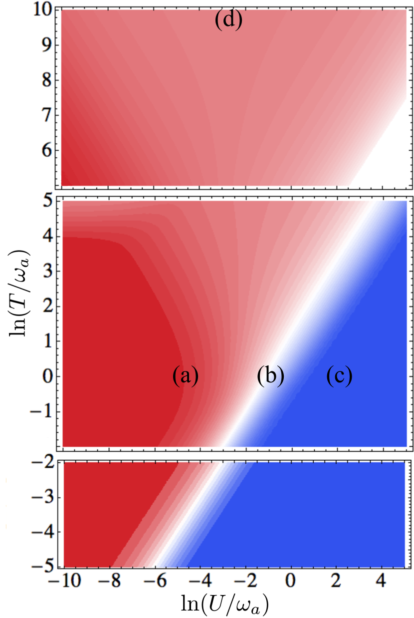
Figure 1: (color online) $g_{a}^{(2)}$ as a function of temperature and nonlinearity for the Kerr Hamiltonian $H_{K}$. Upper panel: the high occupation approximated solution, with the top limit $\pi/2$. Middle panel: Numerical solution. Lower panel: the low occupation approximated solution. Red corresponds to 2, white to 1 and blue to 0. The points marked with letters are further investigated in Fig. 2.

Since $H_{K}$ is diagonal in the resonator number state basis, $\langle m|H_{K}|n\rangle=\delta_{mn}\epsilon_{n}$, calculations are straightforward and even analytical in some limits. For instance, transition energies between the levels with $\epsilon_{n}=n\omega_{a}+n(n-1)U$ and $n=0,1,\ldots$ are simply given by $\Delta\epsilon_{n}=\epsilon_{n}-\epsilon_{n-1}=\omega_{a}+2(n-1)U$, i.e. they increase linearly with $n$ and $U$.

The thermalized state achieved with the standard Kerr-nonlinearity Hamiltonian $H_{K}$ should on physical grounds be given by the canonical ensemble,

$$\rho_{T}=\frac{1}{Z}\sum_{n}e^{-\frac{\omega_{a}n+Un(n-1)}{T}}\left|n\right\rangle\left\langle n\right|$$ (8)

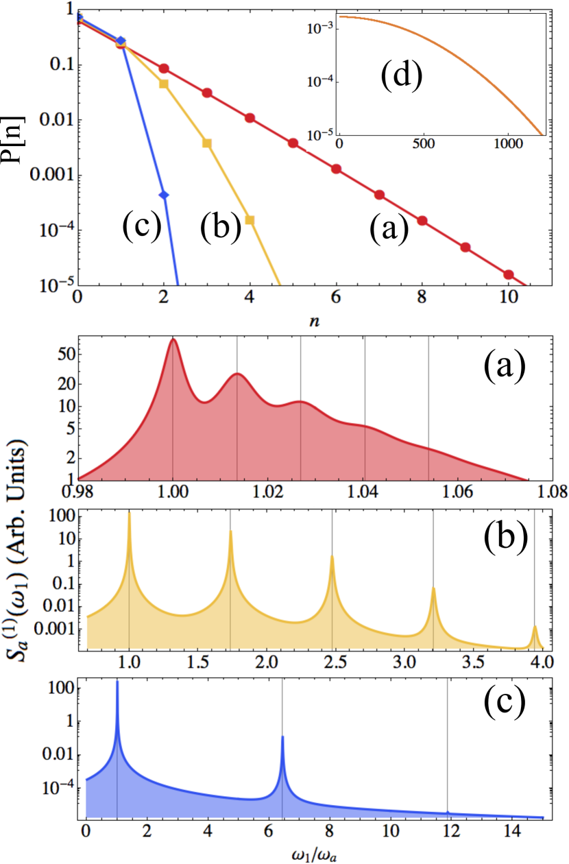
with $Z=\sum_{n}e^{-\frac{\omega_{a}n+Un(n-1)}{T}}$ Alicki . A fundamental difference between Eqs. (6) and (8) is that the first one has particle statistics that are independent of the parameters of the Hamiltonian and even independent of temperature with $g_{a}^{(N)}=\langle(a^{\dagger})^{N}a^{N}\rangle/\langle a^{\dagger}a\rangle^{N}=N!$ while the latter one has particle statistics depending on $T$ and $U$, including subpoissonian regions with $g_{a}^{(2)}<1$ Quattropani . We have plotted $g_{a}^{(2)}$ according to Eq. (8) in Fig. 1 as an illustration of the rich statistics that the nonlinearity $U$ brings. Only in the region $U\ll\omega_{a}$ (case (a)) do we recover statistics of thermal light fields with $g_{a}^{(2)}=2$ while in the opposite regime (case (c)) we recover the two-level system limit $g_{a}^{(2)}=0$ as expected when levels with more than one particle $n>1$ are so high in energy that they cannot be occupied by thermal fluctuations. The corresponding photon-distribution functions, P$[n]=\left\langle n\right|\rho_{T}\left|n\right\rangle$, are plotted in the upper part of Fig. 2, cases (a) and (c) respectively.

It is interesting that the Kerr nonlinearity $H_{K}$ allows for analytical solutions at the low and high temperature limits, as shown in Fig. 1 with separate upper and lower panels. In the high occupation regime, $T\gg\omega_{a}$, mean values of any observable can be obtained by transforming the sums over the number of excitations, $n$, into an integral (continuous variable approximation) giving for instance,

$$\langle a^{\dagger}a\rangle=\frac{1}{2}-\frac{\omega_{a}}{2U}+\frac{\sqrt{\frac{T}{\pi U}}e^{-\frac{(\omega_{a}-U)^{2}}{4TU}}}{1+\mathrm{Erf}(\frac{U-\omega_{a}}{2\sqrt{TU}})}\,,$$ (9)

with a limiting value of $\lim_{T\rightarrow\infty}g^{(2)}=\pi/2$. The corresponding photon-distribution function, case (d), is plotted in the inset of the upper panel in Fig. 2. In the low occupation regime, at temperatures $T<0.3\omega_{a}$, mean values can be obtained by truncating the sums in the excitation number at $n=2$. From this, we can determine analytically the non-linearity for which the statistics become subpoissonian, $g^{(2)}\leq 1$, as,

$$U\geq\frac{T}{2}\mathrm{Ln}\big{(}e^{\omega_{a}/T}-1+\sqrt{e^{2\omega_{a}/T}-2e^{\omega_{a}/T}-1}\big{)}-\frac{\omega_{a}}{2}\,.$$ (10)

Figure 2: (color online) Photon number distribution for the four cases marked in Fig. 1 with letters and the corresponding spectra of emission. Parameters are $\gamma_{a}=0.001\omega_{a}$, $T=\omega_{a}$, $\Gamma_{1}=0$ with (a) $U=e^{-5}\omega_{a}$, (b) $U=e^{-1}\omega_{a}$, (c) $U=e^{2}\omega_{a}$. (d) $T=e^{10}\omega_{a}$, $U=e^{-3}\omega_{a}$. The emission in case (d), not shown, is a large broad peak due to the large temperature-induced decoherence.

In order to look into dynamical observables such as the transient dynamics, $\rho(t)$, towards the thermalized steady state or the spectrum of emission, which depend on $\gamma_{a}$ as well, we need the correct master equation for the Hamiltonian $H_{K}$. Owing to the regime of deep anharmonicity, the standard quantum optical master equation with $\mathcal{\tilde{L}}_{T}$ would give a false description of the dynamics. Indeed, this Lindblad dissipator is obtained in an optical regime where the energy differences between subsequent levels are almost the same, and in this case the mean excitation number in the bath, i.e. the feeding factor, is almost the same for each transition and thus fixed as a constant. In the spirit of Ref. Blais , one can perform a perturbative expansion in the system-bath coupling strength in the basis of the eigenstates $|j\rangle$ of the exact Hamiltonian at hand, $H_{K}$ in this case, in order to derive the Redfield equations breuer that describe the dissipative processes. In our notation, we label the states $|j\rangle$ such that $\omega_{k}>\omega_{j}$ as $k>j$. After some algebra, we obtain a master equation with

$$\mathcal{L}_{T} = \sum_{j,k>j}\Gamma^{jk}_{a}\Big{[}1+\bar{n}_{T}(\Delta_{kj})\Big{]}\mathcal{D}_{|j\rangle\langle k|}$$ (11)

$$+ \sum_{j,k>j}\Gamma^{jk}_{a}\bar{n}_{T}(\Delta_{kj})\mathcal{D}_{|k\rangle\langle j|}\,.$$

In particular, in Eq. (11), $\mathcal{D}$ operates on the transition operators $|k\rangle\langle j|$ between the k-th and j-th eigenstates. The relaxation coefficients $\Gamma^{jk}_{a}=2\pi d_{a}(\Delta_{kj})\alpha^{2}_{a}(\Delta_{kj})|C^{a}_{jk}|^{2}$ can be interpreted as the full width at half maximum of each $|k\rangle\rightarrow|j\rangle$ transition at zero temperature, and they depend on the spectral density of the bath $d_{a}(\Delta_{kj})$ and the strength of the coupling to the bath $\alpha_{a}(\Delta_{kj})$ at their respective transition frequency $\Delta_{kj}=\omega_{k}-\omega_{j}$, as well as on the transition coefficients $C_{jk}=\langle j|(a+a^{\dagger})|k\rangle$. For a flat spectral density $d_{a}(\Delta_{kj})$, and couplings $\alpha_{a}(\Delta_{kj})$ that are frequency independent (Markov approximation), the relaxation coefficients reduce to $\Gamma^{jk}_{a}=\gamma_{a}|C^{a}_{jk}|^{2}$, where $\gamma_{a}$ is the standard damping rate. For the Hamiltonian $H_{K}$, the eigenstates remain the number states $\left|n\right\rangle$ and the energy difference between them is $\Delta\epsilon_{n}$. In order to solve Eq. (4) in the steady state, we first put the density matrix elements $\left\langle j\right|\rho\left|k\right\rangle$ in a vector that we denote $\mathbf{v}$ and rewrite the master equation in matricial form,

$$\partial_{\tau}\mathbf{v}(\tau)=M\mathbf{v}(\tau)\,.$$ (12)

The transient solution $\mathbf{v}(\tau)=e^{M\tau}\mathbf{v}(0)$ converges to the steady state in the long time limit as

$$\mathbf{v}^{\mathrm{ss}}=\lim_{\tau\rightarrow\infty}\mathbf{v}(\tau)=\lim_{\tau\rightarrow\infty}e^{M\tau}\left(\begin{array}[]{c}1\\ 0\\ \vdots\end{array}\right)\,,$$ (13)

where we have chosen the vacuum as the initial condition. Since we employ the justified assumption of a unique steady state Spohn ; Schirmer , the initial state is irrelevant and all the relevant information is encoded in $e^{M\tau}$. With this, we arrive to the thermal steady state defined by Eq. (8).

From the dynamics, we additionally obtain the spectrum of emission in the steady state (set at $t=0$),

$$S_{a}^{(1)}(\omega_{1})=\frac{1}{\pi}\Re\int_{0}^{\infty}d\tau e^{-\frac{\Gamma_{1}}{2}\tau}e^{-i\omega_{1}\tau}\langle a^{\dagger}(0)a(\tau)\rangle\,,$$ (14)

using the quantum regression formula delvallebook10 to obtain the two-time correlator $\langle a^{\dagger}(0)a(\tau)\rangle$ from the master equation (12). The linewidth $\Gamma_{1}$ provides the uncertainty in the frequency detection of the measurement apparatus eberly77a . According to Ref. delvalle12a , the spectrum can also be computed as the steady state population of an output detector or sensor with central frequency $\omega_{1}$ which is very weakly coupled to the measured field $a$,

$$S_{a}^{(1)}(\omega_{1})\propto\langle n_{1}\rangle\,,$$ (15)

where $\langle n_{1}\rangle$ is the sensor occupation and $\Gamma_{1}$ its decay rate. In the Appendix we explain in detail the method to compute the spectrum within the density matrix formalism, providing a semi-analytical formula in terms of the matrix $M$, Eq. (28).

Fig. 2 shows three examples of spectra of emission together with the photon number distribution for a fixed temperature and three different nonlinearities, marked in Fig. 1 as (a), (b) and (c). The photon number distribution would be that of (a) for the three cases, had we solved the master equation with Liouvillian $\mathcal{\tilde{L}}_{T}$ given in Eq. (5). The proper Liouvillian, Eq. (11), gives rise to a distribution that is $U$-dependent as required on physical grounds. The spectrum of emission is different in all three cases even under $\mathcal{\tilde{L}}_{T}$, but the intensities of the peaks are not accurately obtained. As expected, increasing the nonlinearity separates the different peaks, produced in the different transitions between subsequent energy levels, and makes it increasingly harder to populate high energy levels. At very large $U$, only the peak at $\omega_{a}$ survives as it corresponds to the emission of a two-level system.

IV Full anharmonic Hamiltonian

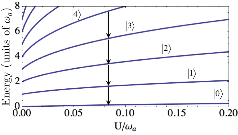
Figure 3: Energy levels of $H_{S}$ as a function of the nonlinearity $U$ for repulsive nonlinearities $U>0$.

For higher photon numbers, a more accurate description of the ultra-anharmonic regime is provided by the Hamiltonian $H_{S}$. After the diagonalization of $H_{S}$, whose eigenstates are no longer the number states, the steady state density matrix of the canonical ensemble reduces to,

$$\rho_{T}=\frac{1}{Z}\sum_{j}e^{-\epsilon_{j}/T}\left|j\right\rangle\left\langle j\right|$$ (16)

where $\epsilon_{j}$ is the j-th eigenvalue of $H_{S}$ and $Z=\sum_{j}e^{-\epsilon_{j}/T}$. These eigenenergies are plotted in Fig. 3 as a function of the nonlinearity. In this case, not only the dissipation term in the master equation but also the photodetection has to be modified in order to correctly describe the nonlinearity of the system RidolfoPrl2012 . Otherwise, unphysical results are found such as a stream of output photons when the system is in its ground state Werlang . By following the original photodetection formulation by Glauber, the probability per second that a photon is absorbed by an ideal detector is proportional to $\langle E^{-}(t)E^{+}(t)\rangle$, where $E^{\pm}(t)$ are the positive and negative frequency components of the electric field operator of the output. In the same way, the photon correlation functions are straightforwardly calculated as Milonni ; SavastaPRA1996 $\langle E^{-}(t)E^{-}(t^{\prime})E^{+}(t^{\prime})E^{+}(t)\rangle$, with all the positive frequency operators to the right and all the negative frequency operators to the left. Following Ref. RidolfoPrl2012 , by expressing the cavity electric-field operator in the eigenbasis, we derive correlation functions for the output fields which are valid for an arbitrary nonlinearity. Let us define the quadrature operators $X=X_{0}(a+a^{\dagger})$, and its conjugate momentum $P=-iP_{0}(a-a^{\dagger})$, with their time derivatives, $\dot{X}=i[H,X]$ and $\dot{P}=i[H,P]$. The input-output relations can be derived in a very general way GardinerZoller , and for an $X$ quadrature coupled to the electric field of the output channel, one finds,

$$E_{\text{out}}=E_{\text{in}}-\sqrt{\kappa}\,\dot{X}$$ (17)

where $\kappa$ is the associated decay rate into the output channel. Likewise, Eq. (17) can be generalized for the $P$ quadrature just replacing $X$ with $P$. Although this latter replacement seems to be harmless, it is worthwhile to notice that it has crucial significance in terms of physical observables. In fact, the output field has to reflect the symmetries of the system as it is explained further on. For input fields in the vacuum state, we define the delayed second order correlation function as

$$g_{\dot{X}}^{(2)}(\tau)=\lim_{t\to\infty}\frac{\langle\dot{X}^{-}(t)\dot{X}^{-}(t+\tau)\dot{X}^{+}(t+\tau)\dot{X}^{+}(t)\rangle}{\langle\dot{X}^{-}(t)\dot{X}^{+}(t)\rangle^{2}}.$$ (18)

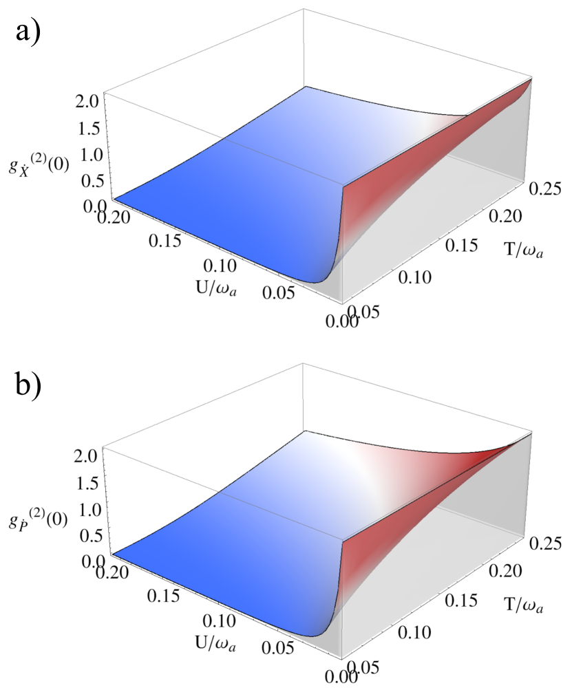
Thus, obtaining the photon correlations for the output fields requires calculating the positive and negative frequency components of the operator $\dot{X}$, namely $\dot{X}^{+}$ and $\dot{X}^{-}$ RidolfoPrl2012 . By expanding $\dot{X}$ in the basis of energy eigenstates $|j\rangle$, it is easy to find $\dot{X}^{+}=-i\sum_{j,k>j}\Delta_{kj}X_{jk}|j\rangle\langle k|$, where $X_{jk}=\langle j|X|k\rangle$ and $\dot{X}^{-}=(\dot{X}^{+})^{\dagger}$. In Fig. 4 we plot the second order coherence function at zero delay for both quadratures, $X$ and $P$. We observe similar behaviors with thermal and antibunched regions for small and large nonlinearities respectively. These functions are always bounded between 0 and 2 as in Fig. 1 and thus show physically meaningful results.

Figure 4: (color online) Zero-delay second order correlation function, $g^{(2)}(0)$, at thermal equilibrium, calculated separating positive and negative frequency components with respect to $H_{S}$ for the $\dot{X}$ quadrature (plot a), i.e. $\langle\dot{X}^{-}\dot{X}^{-}\dot{X}^{+}\dot{X}^{+}\rangle/\langle\dot{X}^{-}\dot{X}^{+}\rangle^{2}$, and for the $\dot{P}$ quadrature (pot b).

Let us finally turn into steady state spectral functions for one and two photons. Here, we couple the sensors to the $X$ operator, and we easily find the input-output relations for the electric field of the sensors as in Eq. (17). Since the sensors are very weakly coupled to the system, we can describe them as a single mode resonance, and the derivative of these operators reduces to $\dot{\varsigma_{i}}=-i\omega_{i}\varsigma_{i}$, being $\omega_{i}$ the frequency of the i-th sensor. Then, the output electric field is just,

$$E_{\text{out}}=E_{\text{in}}-i\,\epsilon_{i}\,\omega_{i}\,X$$ (19)

where $\epsilon_{i}$ is the coupling strength between the i-th sensor and the oscillator. Thus the power spectrum reads,

$$S_{X}^{(1)}(\omega_{1})=\frac{\omega_{1}^{2}}{\pi}\Re\int_{0}^{\infty}d\tau e^{-\frac{\Gamma_{1}}{2}\tau}e^{-i\omega_{1}\tau}\langle X^{-}(0)X^{+}(\tau)\rangle\,,$$ (20)

and the normalized two-photon spectrum of emission, computed as the cross intensity-intensity correlations between two sensors with frequencies $\omega_{1}$ and $\omega_{2}$ read,

$$g_{X}^{(2)}(\omega_{1};\omega_{2})=\frac{S_{X}^{(2)}(\omega_{1};\omega_{2})}{S_{X}^{(1)}(\omega_{1})S_{X}^{(1)}(\omega_{2})}=\frac{\langle n_{1}n_{2}\rangle}{\langle n_{1}\rangle\langle n_{2}\rangle}\,.$$ (21)

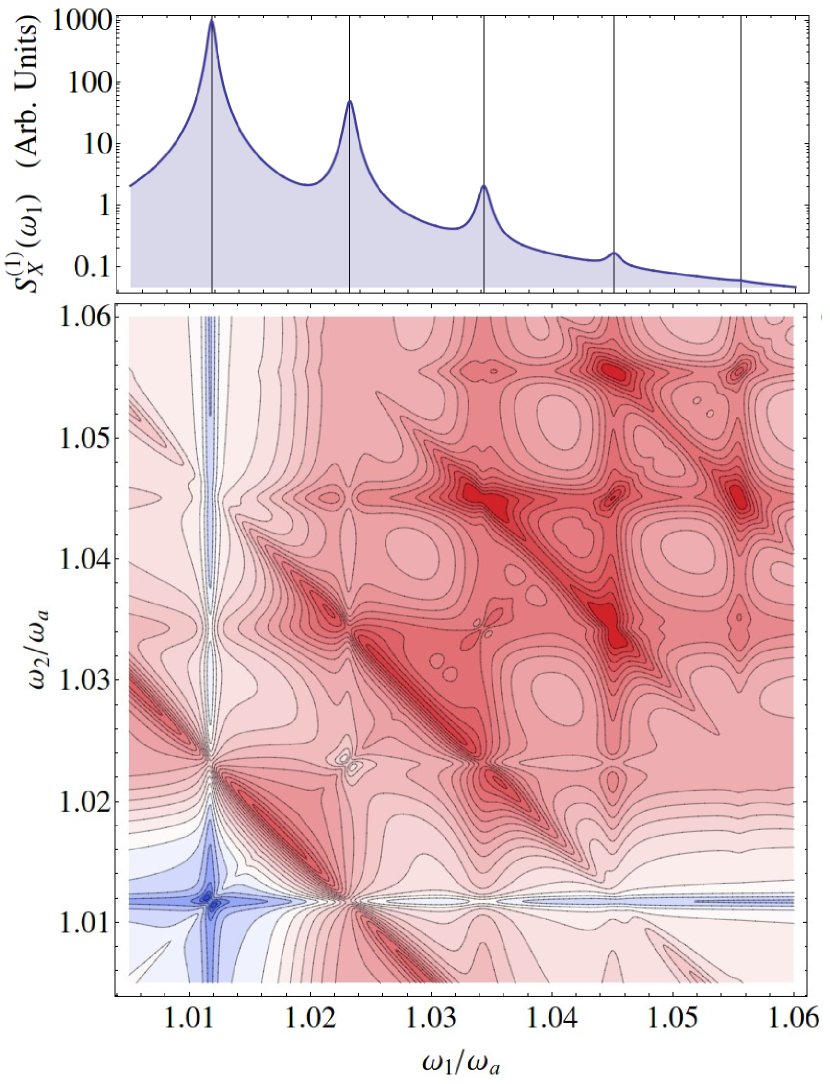
In the Appendix we derive semi-analytical expressions for both the one and two-photon spectrum in the steady state as a function of the master equation coefficient matrix of the system only, $M$, Eq. (36). We plot both $S_{X}^{(1)}(\omega_{1})$ and $g_{X}^{(2)}(\omega_{1};\omega_{2})$ in Fig. 5 for the full Hamiltonian $H_{S}$ in a region where the mean number of excitations is $\langle X^{-}X^{+}\rangle=0.035$ and the total second order coherence function is very close to thermal, $g_{\dot{X}}^{(2)}(0)=1.943$. The one-photon spectrum provides again the transition energies in the system and their frequency uncertainty (once deconvoluted from the detector precision $\Gamma_{1}$). The two-photon spectrum provides a clear picture of the level structure gonzaleztudela13a . First, we observe the characteristic blue butterfly shape around each transition frequency, $\omega_{1}=\omega_{2}=\Delta_{j+1j}$, as they are isolated from the rest by the nonlinearity. This is specially visible for the single excitation to ground state transition, $\omega_{1}=\omega_{2}=\Delta_{10}\approx\omega_{a}$, where antibunching is strong (in deep blue color). At larger nonlinearities $U$, this is the only remaining feature as it corresponds to the two-level system. Second, we observe the cascade type of correlations for every pair of consecutive transition frequencies, $\omega_{1}=\Delta_{j+11}$, $\omega_{2}=\Delta_{jj-1}$. This is recognized by a dip in the correlations, as compared to the antidiagonal lines that cross these points, getting close to one. This is the middle value for $g^{(2)}$ at $\tau=0$, between the bunching effect when the sign of the delay follows the natural cascade order (first $\Delta_{j+11}$ and then $\Delta_{jj-1}$) and the opposite delay sign that produces an antibunching effect. Finally, the diagonal and antidiagonal patterns are filtering induced effects. The diagonal line corresponds to an extra bunching produced by measuring indistinguishable photons, $\omega_{1}=\omega_{2}$, as explained in detail in Refs. delvalle12a and gonzaleztudela13a . The antidiagonal lines, given by $\omega_{1}+\omega_{2}=\epsilon_{j}-\epsilon_{j-2}$ for $j\geq 2$, correspond to leapfrog processes, where two-photons are emitted at the same time (within the time uncertainty window $1/\Gamma_{1}$) without populating the intermediate level. The nonlinearity allows these antidiagonal lines to split and be individually resolved, opening, therefore, the possibility of two-photon state generation in the system delvalle13a .

Figure 5: (color online) One-photon spectrum (top panel), and two photon spectrum at zero-delay time (bottom panel) at thermal equilibrium, calculated from Eqs. (28) and (36). Parameters are: $U=10^{-3}\omega_{a}$, $T=0.3\omega_{a}$, $\gamma_{a}=10^{-4}\omega_{a}$, $\Gamma_{1}=\Gamma_{2}=5\times 10^{-4}\omega_{a}$. The vertical grid lines mark the positions of the transitions in the system. The color scale ranks from the minimum to maximum value: 0.063 (darkest) blue, 1 white, 1572 (darkest) red.

V Attractive Nonlinearities

Circuit quantum electrodynamics is a prime candidate for the realization of attractive ($U<0$) ultra strong optical nonlinearities of the form we investigate here. We thus complete our discussion with results for an attractive nonlinearity, $U<0$, as it is for example realized in transmon qubits Koch07 or in a transmission line resonator where the central conductor is intersected by a dc SQUID Leib12 ; Bourassa12 .

A version of the Hamiltonian (1) can be implemented for microwave fields in circuit quantum electrodynamics where the nonlinearity is provided by a Josephson junction. The associated nonlinear inductance is described by a term $E_{J}\cos\phi$ in the Hamiltonian, which yields the Hamiltonian (1) by identifying $\phi=\sqrt{2E_{C}/E_{J}}\left(a+a^{\dagger}\right)$, $\omega_{a}=\sqrt{8E_{C}E_{J}}$ and $U_{2n}=-E_{J}\left(-2E_{C}/E_{J}\right)^{n}/(2n)!$ Leib12 , where $E_{C}$ and $E_{J}$ are the charging and Josephson energies of the considered circuit. Here, $U=-E_{C}/12$ is negative and the power series in Eq. (1) can only be truncated for sufficiently small ratios $E_{C}/E_{J}$ as for example in a transmon Koch07 .

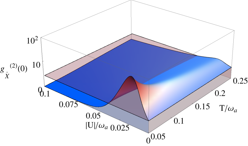
Fig. 6 shows $g_{\dot{X}}^{(2)}(0)$ according to Eq. (8) for the case where $U<0$. For comparison we also show the plane $g_{\dot{X}}^{(2)}(0)=2$ for standard thermal particle statistics of a non-interacting field. One can clearly identify a region with enhanced bunching $g_{\dot{X}}^{(2)}(0)>2$ for moderate but nonzero interactions and low temperatures. For stronger interactions $|U|/\omega_{a}\gtrsim 0.04$ the field becomes strongly antibunched. Note that we have kept here the next order $U_{6}$ of the nonlinearity to ensure that the spectrum of $H_{S}$ always has a lower bound.

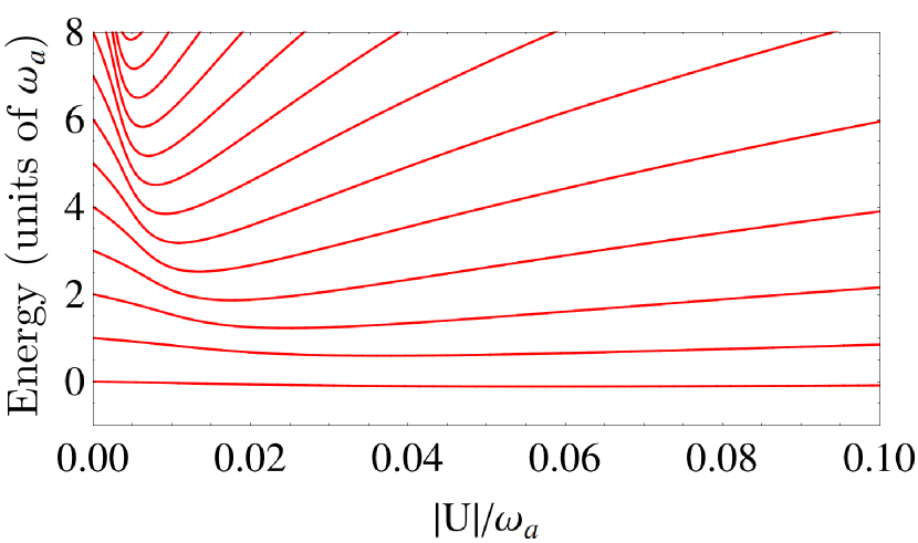
These features can be well understood by inspection of the energy levels of $H_{S}$ as a function of the nonlinearity $|U|$, see Fig. 7. In the parameter region where bunching appears, the transition energy between the first and second excited state is smaller than between ground and first excited state.

Figure 6: (color online) $g_{\dot{X}}^{(2)}(0)$ as a function of temperature and nonlinearity for the Hamiltonian $H_{S}$ (including the corresponding $U_{6}$-term) with $U<0$, c.f. Eq. (2). For comparison we show the plane $g_{\dot{X}}^{(2)}(0)=2$ for standard thermal particle statistics of a non-interacting field.

Figure 7: Energy levels of $H_{S}$ (including the corresponding $U_{6}$-term) as a function of the nonlinearity $U$ for attractive nonlinearities $U<0$.

VI Conclusions

We have analyzed the effect of a nonlinearity, $U$, that can be as large as the natural frequency, $\omega_{a}$, on the thermal equilibrium properties of a single mode. We have considered two types of quartic nonlinearities in the Hamiltonian of the system and derived the adequate master equation for the time evolution in contact with the thermal bath, as well as the output fields that can be measured in each case. In order to obtain a physical solution in agreement with the canonical ensemble, the Lindblad forms that describe dissipation and excitation must be in terms of the new eigenstates of the Hamiltonian, which are obtained numerically beforehand. We have focused on spectral and statistical properties of the system in a separated (one-photon or power spectrum of emission and second order coherence function) and combined (frequency resolved second order correlations or two-photon spectrum) way. We have derived a semi-analytical expression for the last one, following a sensor approach, only in terms of the master equation coefficients and the steady state density matrix. These observables offer complementary information about the different regimes appearing in the system when varying $U/\omega_{a}$ and $T/\omega_{a}$. At small nonlinearities the mode is in a thermal state, $g^{(2)}=2$, and one can apply the standard approximations for the Lindblad terms and output field. At large nonlinearities, however, the behavior is effectively close to that of a two-level system, with antibunched statistics, $g^{(2)}=0$, and a single transition isolated in energy. In the intermediate regimes a cascade of well defined transitions occurs providing a set of peaks in the spectrum and $0<g^{(2)}<2$. For attractive nonlinearities, $U<0$, low temperatures and small interactions, bunching can be enhanced above the thermal value, $g^{(2)}>2$.

Appendix A Derivation and formulas for one- and two-photon spectrum

Following the general formalism in Ref. delvalle12a , we derive semi-analytical expressions for the steady state one- and two-photon spectra of emission from a master equation approach, in an analogous way as done in Ref. gonzaleztudela13a , in terms of the relevant correlators in the system and their equations. We call the measured annihilation and creation field operators $X^{+}$ and $X^{-}$.

We define two reordering matrices, $T_{\pm}$, which, when acting on $\mathbf{v}$, substitute each element in it, $\left\langle m\right|\rho\left|n\right\rangle$, by $\left\langle m\right|X^{+}\rho\left|n\right\rangle$ for $T_{+}$ and $\left\langle m\right|\rho X^{-}\left|n\right\rangle$ for $T_{-}$. These matrices always exist, in infinite or in truncated Hilbert spaces (where, if truncation is to order $n_{\mathrm{max}}$, we set $\left\langle n_{\mathrm{max}}\right|X^{+}\rho\left|n\right\rangle=0$ and $\left\langle n\right|\rho X^{-}\left|n_{\mathrm{max}}\right\rangle=0$ for all $n$).

We now consider two sensors (although this can be generalized to an arbitrary number) with operators $\varsigma_{i}$, $i=1,2$ and linewidths $\Gamma_{i}$ coupled to the system with strength $\varepsilon_{i}$ such that the dynamics of the system is probed but is otherwise left unperturbed. This requires the tunnelling rates $\varepsilon_{i}$ to fulfill $\varepsilon_{i}\ll\sqrt{\Gamma_{i}\gamma_{Q}/2}$, where $\gamma_{Q}$ is the smallest system decay rate. The new density matrix that includes the sensors, $\rho_{\mathrm{sen}}$, follows a modified master equation where the photonic tunnelling terms, $H_{\mathrm{sen}}=\sum_{i=1}^{N}[\omega_{i}{\varsigma_{i}^{\dagger}}\varsigma_{i}+\varepsilon_{i}(X^{+}{\varsigma_{i}^{\dagger}}+X^{-}\varsigma_{i})]$, are added to the original Hamiltonian, and the sensor decay terms $\sum_{i=1}^{N}\Gamma_{i}\mathcal{D}_{\varsigma_{i}}\rho_{\mathrm{sen}}$ are added to the dissipative part.

We define new vectors, $\mathbf{w}$, each of them containing the system density matrix (in the same order as $\mathbf{v}$) but for a given combination of sensor states. That is, $\mathbf{w}[\mu_{1}\nu_{1}][\mu_{2}\nu_{2}]$ contains elements $\left\langle j,\mu_{1},\mu_{2}\right|\rho_{\mathrm{sen}}\left|k,\nu_{1},\nu_{2}\right\rangle$ with $j,k=1,2,\ldots$ labelling the system eigenstates. The sensors are two-level systems so the indices $\mu_{i}$ and $\nu_{i}$ take the values 0 or 1. The reduced system density matrix is recovered tracing over the sensors as $\mathbf{v}=\sum_{\mu_{1}=0,1}\sum_{\mu_{2}=0,1}\mathbf{w}[\mu_{1}\mu_{1}][\mu_{2}\mu_{2}]$. The reduced sensor density matrix, is obtained by tracing over the system as $u[\mu_{1}\nu_{1}][\mu_{2}\nu_{2}]=\sum_{m}\left\langle m,\mu_{1},\mu_{2}\right|\rho_{\mathrm{sen}}\left|m,\nu_{1},\nu_{2}\right\rangle=\mathrm{Tr}_{\mathrm{sys}}(\mathbf{w}[\mu_{1}\mu_{1}][\mu_{2}\mu_{2}])$ (noting that $\mathbf{w}$ is a vector so tracing means reconstructing it in a matrix form first). Let us also note that $\mathbf{w}[\mu_{1}\nu_{1}]=\sum_{\mu_{2}=0,1}\mathbf{w}[\mu_{1}\nu_{1}][\mu_{2}\mu_{2}]$ when we trace over the second sensor only.

The part of the master equation concerning each of the sensors and their coupling to the system, reads,

$$\partial_{t}\left\langle m,\mu_{1}\right|\rho_{\mathrm{sen}}\left|n,\nu_{1}\right\rangle\Big{|}_{\mathrm{sensor1}}= [(\nu_{1}-\mu_{1})i\omega_{1}-(\mu_{1}+\nu_{1}){\frac{\Gamma_{1}}{2}}]\left\langle m,\mu_{1}\right|\rho_{\mathrm{sen}}\left|n,\nu_{1}\right\rangle$$ (22a)

$$+\Gamma_{1}(1-\mu_{1})(1-\nu_{1})\left\langle m,1\right|\rho_{\mathrm{sen}}\left|n,1\right\rangle$$ (22b)

$$+i\varepsilon_{1}\Big{[} -\mu_{1}\left\langle m,0\right|X^{+}\rho_{\mathrm{sen}}\left|n,\nu_{1}\right\rangle+\nu_{1}\left\langle m,\mu_{1}\right|\rho_{\mathrm{sen}}X^{-}\left|n,0\right\rangle$$ (22c)

$$-(1-\mu_{1})\left\langle m,1\right|X^{-}\rho_{\mathrm{sen}}\left|n,\nu_{1}\right\rangle+(1-\nu_{1})\left\langle m,\mu_{1}\right|\rho_{\mathrm{sen}}X^{+}\left|n,1\right\rangle\Big{]}\,.$$ (22d)

The sensors are mere spectators of the emission from the system and do not alter its dynamics in any way. They are barely populated ($\langle{\varsigma_{i}^{\dagger}}\varsigma_{i}\rangle\ll 1$) and we can make the approximation that their ground state provides the system steady state (to second order in the couplings): $\mathbf{v}\approx\mathbf{w}[00][00]$. In the same way, tracing over the state of one sensor (for instance, the second) can be achieved by just fixing it in its ground state: $\mathbf{w}[\mu_{1}\nu_{1}]\approx\mathbf{w}[\mu_{1}\nu_{1}][00]$.

In order to obtain the equations of motion valid to leading order in $\varepsilon_{1,2}$, we note that the line b in Eq. (22) only applies to the element where $\mu_{1},\nu_{1}=0$, which is of no interest for us (and we know corresponds to the steady state of the system anyway). We can drop that line for our considerations. Furthermore, the last line d, can be dropped as well because it links the element with $\mu_{1}$ or $\nu_{1}=0$ to $\mu_{1}$ or $\nu_{1}=1$. This would lead to elements of higher order in the couplings, which we discard. In physical terms, line d corresponds to the process of the system absorbing an excitation from the sensors (back action), which we neglect. Therefore, we only keep lines a and c, obtaining, for the two sensor vector,

$$\partial_{t}\mathbf{w}[\mu_{1}\nu_{1}][\mu_{2}\nu_{2}]=\large\{M+[(\nu_{1}-\mu_{1})i\omega_{1}-(\mu_{1}+\nu_{1}){\frac{\Gamma_{1}}{2}}+(\nu_{2}-\mu_{2})i\omega_{2}-(\mu_{2}+\nu_{2})\frac{\Gamma_{2}}{2}]\mathbf{1}\large\}\mathbf{w}[\mu_{1}\nu_{1}][\mu_{2}\nu_{2}]\\ +\mu_{1}(-i\varepsilon_{1}T_{+})\mathbf{w}[0\nu_{1}][\mu_{2}\nu_{2}]+\nu_{1}(i\varepsilon_{1}T_{-})\mathbf{w}[\mu_{1}0][\mu_{2}\nu_{2}]+\mu_{2}(-i\varepsilon_{2}T_{+})\mathbf{w}[\mu_{1}\nu_{1}][0\nu_{2}]+\nu_{2}(i\varepsilon_{2}T_{-})\mathbf{w}[\mu_{1}\nu_{1}][\mu_{2}0]\,.$$ (23)

The matrix $M$ contains the system dynamics. This is equivalent to Eq. (12) of the supplemental material in Ref. delvalle12a . The equations can be solved recursively,

$$\mathbf{w}[\mu_{1}\nu_{1}][\mu_{2}\nu_{2}]=\frac{-1}{M+[(\nu_{1}-\mu_{1})i\omega_{1}-(\mu_{1}+\nu_{1})\frac{\Gamma_{1}}{2}+(\nu_{2}-\mu_{2})i\omega_{2}-(\mu_{2}+\nu_{2})\frac{\Gamma_{2}}{2}]\mathbf{1}}\\ \times\Big{\{}\mu_{1}(-i\varepsilon_{1}T_{+})\mathbf{w}[0\nu_{1}][\mu_{2}\nu_{2}]+\nu_{1}(i\varepsilon_{1}T_{-})\mathbf{w}[\mu_{1}0][\mu_{2}\nu_{2}]+\mu_{2}(-i\varepsilon_{2}T_{+})\mathbf{w}[\mu_{1}\nu_{1}][0\nu_{2}]+\nu_{2}(i\varepsilon_{2}T_{-})\mathbf{w}[\mu_{1}\nu_{1}][\mu_{2}0]\Big{\}}\,.$$ (24)

A.1 One-photon spectrum of emission (one sensor)

The single-photon physical spectrum of the field $X$ is given in the steady state (set at $t=0$) by Eq. (20) in the main text, that is, by the average population, in the steady state, of any one of the two sensors, say, the first one,

$$\langle n_{1}\rangle=\langle\varsigma^{\dagger}_{1}\varsigma_{1}\rangle=\mathrm{Tr}_{\mathrm{sys}}(\mathbf{w}[11][00])=\frac{\varepsilon_{1}^{2}}{\Gamma_{1}}(2\pi)S_{\Gamma_{1}}^{(1)}(\omega_{1})\,,$$ (25)

as was proven in Ref. delvalle12a . The approximated equation of motion of such element, reads $\partial_{t}\mathbf{w}[11][00]=(M-\Gamma_{1}\mathbf{1})\mathbf{w}[11][00]+(-i\varepsilon_{1}T_{+})\mathbf{w}[01][00]+(i\varepsilon_{1}T_{-})\mathbf{w}[10][00]$, so we have,

$$\mathbf{w}[11][00]=\frac{-1}{M+(-\Gamma_{1})\mathbf{1}}\Big{\{}(-i\varepsilon_{1}T_{+})\mathbf{w}[01][00]+(i\varepsilon_{1}T_{-})\mathbf{w}[10][00]\Big{\}}\,.$$ (26)

Using the solution Eq. (24), the elements of interest for the spectrum read,

$$\mathbf{w}[01][0,0]=\frac{-1}{M+(i\omega_{1}-\frac{\Gamma_{1}}{2})\mathbf{1}}(i\varepsilon_{1}T_{-})\mathbf{v}^{\mathrm{ss}}\,,$$ (27a)

$$\mathbf{w}[10][0,0]=\frac{-1}{M+(-i\omega_{1}-\frac{\Gamma_{1}}{2})\mathbf{1}}(-i\varepsilon_{1}T_{+})\mathbf{v}^{\mathrm{ss}}\,.$$ (27b)

The final expression is,

$$\langle n_{1}\rangle=\varepsilon_{1}^{2}\,\mathrm{Tr}_{\mathrm{sys}}\Big{(}\frac{1}{M+(-\Gamma_{1})\mathbf{1}}\Big{[}T_{+}\frac{1}{M+(i\omega_{1}-\frac{\Gamma_{1}}{2})\mathbf{1}}T_{-}+T_{-}\frac{1}{M+(-i\omega_{1}-\frac{\Gamma_{1}}{2})\mathbf{1}}T_{+}\Big{]}\mathbf{v}^{\mathrm{ss}}\Big{)}\,.$$ (28)

A.2 Two-photon spectrum of emission (two sensors)

The physical two-photon spectrum in the steady state and at $\tau=0$, is given by intensity-intensity cross correlations between two sensors as

$$\langle n_{1}n_{2}\rangle=\langle\varsigma^{\dagger}_{1}\varsigma_{1}\varsigma^{\dagger}_{2}\varsigma_{2}\rangle=\mathrm{Tr}_{\mathrm{sys}}(\mathbf{w}[11][11])=\frac{\varepsilon_{1}^{2}\varepsilon_{2}^{2}}{\Gamma_{1}\Gamma_{2}}(2\pi)^{2}S_{\Gamma_{1}\Gamma_{2}}^{(2)}(\omega_{1};\omega_{2})\,,$$ (29)

with,

$$\mathbf{w}[11][11]=\frac{-1}{M+(-\Gamma_{1}-\Gamma_{2})\mathbf{1}}\Big{\{}(-i\varepsilon_{2}T_{+})\mathbf{w}[11][01]+(i\varepsilon_{2}T_{-})\mathbf{w}[11][10]+\left[1\leftrightarrow 2\right]\Big{\}}\,.$$ (30)

This solution relies on $\mathbf{w}[11][01]$ and $\mathbf{w}[11][10]$, which can be expressed in terms of four lower order correlators:

$$\mathbf{w}[11][01]=\frac{-1}{M+(i\omega_{2}-\Gamma_{1}-\frac{\Gamma_{2}}{2})\mathbf{1}}\Big{\{}i\varepsilon_{2}T_{-}\mathbf{w}[11][00]+i\varepsilon_{1}T_{-}\mathbf{w}[10][01]-i\varepsilon_{1}T_{+}\mathbf{w}[01][01]\Big{\}}\,,$$ (31)

and

$$\mathbf{w}[11][10]=\frac{-1}{M+(-i\omega_{2}-\Gamma_{1}-\frac{\Gamma_{2}}{2})\mathbf{1}}\Big{\{}-i\varepsilon_{2}T_{+}\mathbf{w}[11][00]+i\varepsilon_{1}T_{-}\mathbf{w}[10][10]-i\varepsilon_{1}T_{+}\mathbf{w}[01][10]\Big{\}}\,.$$ (32)

Their solutions are Eq. (26) and

$$\mathbf{w}[10][01]=\frac{-1}{M+(-i\omega_{1}+i\omega_{2}-\frac{\Gamma_{1}+\Gamma_{2}}{2})\mathbf{1}}\Big{\{}i\varepsilon_{2}T_{-}\mathbf{w}[10][00]-i\varepsilon_{1}T_{+}\mathbf{w}[00][01]\Big{\}}\,,$$ (33)

and

$$\mathbf{w}[01][01]=\frac{-1}{M+(i\omega_{1}+i\omega_{2}-\frac{\Gamma_{1}+\Gamma_{2}}{2})\mathbf{1}}\Big{\{}i\varepsilon_{1}T_{-}\mathbf{w}[00][01]-i\varepsilon_{2}T_{-}\mathbf{w}[01][00]\Big{\}}\,.$$ (34)

and

$$\mathbf{w}[10][10]=\frac{-1}{M+(-i\omega_{1}-i\omega_{2}-\frac{\Gamma_{1}+\Gamma_{2}}{2})\mathbf{1}}\Big{\{}-i\varepsilon_{1}T_{+}\mathbf{w}[00][10]-i\varepsilon_{2}T_{+}\mathbf{w}[10][00]\Big{\}}\,.$$ (35)

By recurrence, we can build the final solution in terms of the system master equation, $M$, and the sensor parameters directly,

$$\langle n_{1}n_{2}\rangle= \epsilon_{1}^{2}\epsilon_{2}^{2}\,\mathrm{Tr}_{\mathrm{sys}}\Big{(}\frac{1}{M+(-\Gamma_{1}-\Gamma_{2})\mathbf{1}}$$

$$\times\Big{\{}T_{+}\frac{1}{M+(i\omega_{2}-\Gamma_{1}-\frac{\Gamma_{2}}{2})\mathbf{1}}\Big{[} T_{-}\frac{1}{M-\Gamma_{1}\mathbf{1}}\Big{(}T_{+}\frac{1}{M+(i\omega_{1}-\frac{\Gamma_{1}}{2})\mathbf{1}}T_{-}+T_{-}\frac{1}{M+(-i\omega_{1}-\frac{\Gamma_{1}}{2})\mathbf{1}}T_{+}\Big{)}$$

$$+ T_{-}\frac{1}{M+(-i\omega_{1}+i\omega_{2}-\frac{\Gamma_{1}+\Gamma_{2}}{2})\mathbf{1}}\Big{(}T_{-}\frac{1}{M+(-i\omega_{1}-\frac{\Gamma_{1}}{2})\mathbf{1}}T_{+}+T_{+}\frac{1}{M+(i\omega_{2}-\frac{\Gamma_{2}}{2})\mathbf{1}}T_{-}\Big{)}$$

$$+ T_{+}\frac{1}{M+(i\omega_{1}+i\omega_{2}-\frac{\Gamma_{1}+\Gamma_{2}}{2})\mathbf{1}}\Big{(}T_{-}\frac{1}{M+(i\omega_{2}-\frac{\Gamma_{2}}{2})\mathbf{1}}T_{-}+T_{-}\frac{1}{M+(i\omega_{1}-\frac{\Gamma_{1}}{2})\mathbf{1}}T_{-}\Big{)}\Big{]}$$

$$+T_{-}\frac{1}{M+(-i\omega_{2}-\Gamma_{1}-\frac{\Gamma_{2}}{2})\mathbf{1}}\Big{[} T_{+}\frac{1}{M-\Gamma_{1}\mathbf{1}}\Big{(}T_{+}\frac{1}{M+(i\omega_{1}-\frac{\Gamma_{1}}{2})\mathbf{1}}T_{-}+T_{-}\frac{1}{M+(-i\omega_{1}-\frac{\Gamma_{1}}{2})\mathbf{1}}T_{+}\Big{)}$$

$$+ T_{-}\frac{1}{M+(-i\omega_{1}-i\omega_{2}-\frac{\Gamma_{1}+\Gamma_{2}}{2})\mathbf{1}}\Big{(}T_{+}\frac{1}{M+(-i\omega_{2}-\frac{\Gamma_{2}}{2})\mathbf{1}}T_{+}+T_{+}\frac{1}{M+(-i\omega_{1}-\frac{\Gamma_{1}}{2})\mathbf{1}}T_{+}\Big{)}$$

$$+ T_{+}\frac{1}{M+(i\omega_{1}-i\omega_{2}-\frac{\Gamma_{1}+\Gamma_{2}}{2})\mathbf{1}}\Big{(}T_{-}\frac{1}{M+(-i\omega_{2}-\frac{\Gamma_{2}}{2})\mathbf{1}}T_{+}+T_{+}\frac{1}{M+(i\omega_{1}-\frac{\Gamma_{1}}{2})\mathbf{1}}T_{-}\Big{)}\Big{]}$$

$$+[1\leftrightarrow 2]\Big{\}}\mathbf{v}^{\mathrm{ss}}\Big{)}\,.$$ (A15)

References

• (1) D. F. Walls and G. J. Milburn, Quantum Optics (Cambridge University Press, Cambridge, England, 1994).
• (2) G. Günter et al., Nature 458, 178 (2009).
• (3) T. Niemczyk et al., Nat. Phys. 6, 772 (2010).
• (4) Y. Todorov et al., Phys. Rev. Lett. 105, 196402 (2010).
• (5) T. Schwartz, J. A. Hutchison, C. Genet, and T. W. Ebbesen, Phys. Rev. Lett. 106, 196405 (2011).
• (6) A.J. Hoffman et al., Phys. Rev. Lett. 107, 053602 (2011).
• (7) G. Scalari et al., Science 16, 1323 (2012).
• (8) A. Ridolfo, M. Leib, S. Savasta, and M. J. Hartmann, Phys. Rev. Lett. 109, 193602 (2012).
• (9) A. Ridolfo, M. Leib, S. Savasta, and M. J. Hartmann, Phys. Scr. T153, 014053 (2013).
• (10) A. Ridolfo, S. Savasta, and M. J. Hartmann, Phys. Rev. Lett. 110, 163601 (2013).
• (11) R. Stassi, A. Ridolfo, O. Di Stefano, M. J. Hartmann, and S. Savasta, Phys. Rev. Lett. 110, 243601 (2013).
• (12) A. Imamoğlu, H. Schmidt, G. Woods and M. Deutsch, Phys. Rev. Lett. 79, 1467 (1997).
• (13) M. O. Scully and M. S. Zubairy, Quantum Optics, (Cambridge University Press, Cambridge, England, 1997)
• (14) P. D. Drummond and D. F. Walls, J. Phys. A: Math. Gen. 13 725 (1980)
• (15) F. Beaudoin, J. M. Gambetta, and A. Blais, Phys. Rev. A 84, 043832 (2011).
• (16) J. Koch, T.M. Yu, J. Gambetta, A.A. Houck, D.I. Schuster, J. Majer, A. Blais, M.H. Devoret, S.M. Girvin, and R.J. Schoelkopf, Phys. Rev. A 76, 042319 (2007).
• (17) M. Leib, F. Deppe, A. Marx, R. Gross, and M. J. Hartmann, New J. Phys. 14, 075024 (2012).
• (18) J. Bourassa, F. Beaudoin, J. M. Gambetta, and A. Blais, Phys. Rev. A 86, 013814 (2012).
• (19) V. Peano and M. Thorwart, New J. Phys. 8, 21 (2006).
• (20) H.-P. Breuer and F.Petruccione, The Theory of Open Quantum Systems, Oxford University Press (2006).
• (21) C. W. Gardiner and P. Zoller, Quantum Noise, Springer-Verlag, (2000).
• (22) R. Alicki, Phys. Rev. A 40, 4077 (1989).
• (23) A. Quattropani, P. Schwendimann, and H. P. Baltes, Optica Acta 27, 135 (1980).
• (24) E. del Valle, Microcavity Quantum Electrodynamics, VDM Verlag (2010).
• (25) H. Spohn, Lett. Math. Phys. 2, 33 (1977)
• (26) S. G. Schirmer and Xiaoting Wang, Phys. Rev. A 81, 062306 (2010)
• (27) J. Eberly and K. Wódkiewicz, J. Opt. Soc. Am. 67, 1252 (1977)
• (28) T. Werlang, A. V. Dodonov, E. I. Duzzioni, and C. J. Villas-Bôas, Phys. Rev. A 78, 053805 (2008).
• (29) P. W. Milonni and D. F. V. James, and H. Fearn, Phys. Rev. A 52, 1525 (1995).
• (30) S. Savasta and R. Girlanda, Phys. Rev. A 53, 2716 (1996).
• (31) E. del Valle, A. Gonzalez-Tudela, F. P. Laussy, C. Tejedor and M. J. Hartmann, Phys. Rev. Lett. 109 183601 (2012)
• (32) A. Gonzalez-Tudela, F. P. Laussy, C. Tejedor, M. J. Hartmann and E. del Valle, New J. Phys. 15, 033036 (2013)
• (33) E. del Valle, New J. Phys. 15, 025019 (2013)