Generalized parton distributions for the proton in AdS/QCD

Abstract

We present a study of proton generalized parton distributions( GPDs) in both momentum and position spaces using the proton wave function obtained from AdS/ QCD. Here we consider the soft wall model. The results are compared with a phenomenological model of proton GPDs.

Introduction

Generalized parton distributions (GPDs) appear in the exclusive processes like deeply virtual Compton scattering (DVCS) or vector meson productions. The GPDs are functions of three variables, namely, longitudinal momentum faction $x$ of the quark or gluon, square of the total momentum transferred ($t$) and the skewness $\zeta$, which represents the longitudinal momentum transferred in the process. The GPDs contain much more informations about the nucleon structure and spin (see rev for example) compared to the ordinary parton distribution functions(pdfs) which are functions of $x$ only. The GPDs reduce to the ordinary parton distributions in the forward limit. Their first moments are related to the form factors and provide interesting information about the spin and orbital angular momentum of the constituents, as well as the spatial structure, of the nucleons. Being off-forward matrix elements, the GPDs have no probabilistic interpretation. But for zero skewness, the Fourier transforms of the GPDs with respect to the transverse momentum transfer ($\Delta_{\perp}$) give the impact parameter dependent GPDs which satisfy the positivity condition and can be interpreted as distribution functions burk1 . The impact parameter dependent GPDs provide us with the information about partonic distributions in the impact parameter or the transverse position space for a given longitudinal momentum ($x$). The impact parameter $b_{\perp}$ gives the separation of the struck quark from the center of momentum. In the $t\to 0$ limit, Ji’s sum rule ji relates the moment of the GPDs to the angular momentum contribution to the nucleon by the quark or gluon. Again in the impact parameter space, the sum rule has a simple interpretation for a transversely polarized state burk . The term containing $E(x,0,0)$ arises due to a transverse deformation of the GPDs in the center of momentum frame, whereas the term containing $H(x,0,0)$ is an overall transverse shift when going from the transversely polarized state in instant form to the front form.

As different experiments have measured or are planned to measure DVCS as well as vector meson production(e.g, HERA H1, COMPASS H1 ; H2 ; COMPASS and ZEUS ZEUS1 ; ZEUS2 collaborations, HARMES HERMES , JLAB CLAS , etc.), there are many activities going on to model GPDs for the proton.

In the overlap representation, GPDs can be expressed as off-forward matrix elements of bilocal light front currents. Using AdS/QCD, one can extract the light front wave functions(LFWFs) for the hadrons and thus provide an interesting way to calculate the GPDs. Polchinski and Strassler PS first used the AdS/CFT duality to address the hard scattering and deep inelastic scattering. The AdS/QCD for the baryon has been developed by several groups BT ; ads1 ; ads2 . Though it gives only the semiclassical approximation of QCD, so far this method has been successfully applied to describe many hadron properties e.g., the hadron mass spectrum, parton distribution functions, meson and nucleon form factors, structure functions etcBT1 ; AC ; BT2 . To describe the Pauli form factor in AdS/QCD, one needs to have nonminimal coupling as proposed by Abidin and Carlson AC . Recently it has been shown that AdS/QCD wave functions remarkably agree with experimental data for $\rho$ meson electroproduction forshaw . AdS/QCD has also been successfully applied in the meson sector to predict the branching ratio for decays of $\bar{B^{0}}$ and $\bar{B_{s}^{0}}$ into $\rho$ mesons ahmady1 , isospin asymmetry and branching ratio for the $B\to K^{*}\gamma$ decays ahmady2 , etc. An interesting study of Ehrenfest correspondence principle and the AdS/QFT duality has been done in glazek . Studies of the nucleon form factors with higher Fock sectors have been done in hf1 . Vega et al. vega proposed a beautiful prescription to extract GPDs from the form factors in AdS/QCD and they have done the GPD calculations using both the hard and soft wall models in AdS/QCD. It has been shown that the form of the confining potential in the soft wall model is unique for both the meson and baryon sectors BTD . In this work, we will provide the results for GPDs using the LFWFs obtained from the AdS/ QCD. We will use the formula for the nucleon form factors in the light front quark model with SU(6) spin flavor symmetry and compare the GPDs in the impact parameter space with a phenomenological model of the GPDs for the proton.

Baryon wave functions from AdS/QCD

In this section we briefly review the derivation of the baryon wave functions in AdS/QCD following Brodsky and Téramond BT ; BT2 . We know that the AdS/CFT correspondence relates a gravitationally interacting theory in anti de Sitter space $AdS_{d+1}$ with a conformal gauge theory in $d$ dimensions residing at the boundary. Since QCD is not a conformal theory, one needs to break the conformal invariance of the above duality to generate a bound state spectrum and to relate with QCD. There are two models in the literature to do so. One is the hard wall model in which the conformal symmetry is broken by introducing a boundary at $z_{0}\sim 1/\Lambda_{QCD}$ in the AdS direction where the wave function is made to vanish. In the soft wall model, the conformal invariance is broken by introducing a confining potential in the action of a Dirac field propagating in $AdS_{d+1}$ space. We will consider the soft model in this paper. The relevant action in the soft model is written asBT2

$$S=\int d^{4}xdz\sqrt{g}\Big{(}\frac{i}{2}\bar{\Psi}e^{M}_{A}\Gamma^{A}D_{M}\Psi-\frac{i}{2}(D_{M}\bar{\Psi})e^{M}_{A}\Gamma^{A}\Psi-\mu\bar{\Psi}\Psi-V(z)\bar{\Psi}\Psi\Big{)},$$ (1)

where $e^{M}_{A}=(z/R)\delta^{M}_{A}$ is the inverse vielbein and $V(z)$ is the confining potential, $R$ is the AdS radius. The corresponding Dirac equation in AdS is given by

$$i\Big{(}z\eta^{MN}\Gamma_{M}\partial_{N}+\frac{d}{2}\Gamma_{z}\Big{)}\Psi-\mu R\Psi-RV(z)\Psi=0.$$ (2)

With $z$ identified as the light front transverse impact variable $\zeta$ which gives the separation of the quark and gluonic constituents in the hadron, it is possible to extract the light front wave functions for the hadron. In $d=4$ dimensions, $\Gamma_{A}=\{\gamma_{\mu},-i\gamma_{5}\}$. The light front wave equation for a baryon in $2\times 2$ spinor representation can be written as

$$\frac{d}{d\zeta}\psi_{+}-\frac{\nu+1/2}{\zeta}\psi_{+}+U(\zeta)\psi_{+}=\cal{M}\psi_{-},$$ (3)

$$-\frac{d}{d\zeta}\psi_{-}-\frac{\nu+1/2}{\zeta}\psi_{-}+U(\zeta)\psi_{-}=\cal{M}\psi_{+},$$ (4)

where $\nu$ is related to the orbital angular momentum by $\nu=L+1$, $U(\zeta)=(R/\zeta)V(\zeta)$ is the effective confining potential in the light front Dirac equation, and $\zeta$ is the light front transverse variable giving the separation of quark and gluonic constituents in the baryon. With $z\to\zeta$, substituting $\Psi(x,\zeta)=e^{-iP\cdot x}\zeta^{2}\psi(\zeta)u(P)$ in Eq.(2), and identifying $\mid\mu R\mid=\nu+1/2$, we arrive at the Eqs(3), and (4). For linear confining potential $U(\zeta)=\kappa^{2}\zeta$, Eqs. (3) and (,4) can be written as

$$\big{(}-\frac{d^{2}}{d\zeta^{2}}-\frac{1-4\nu^{2}}{4\zeta^{2}}+\kappa^{4}\zeta^{2}+2(\nu+1)\kappa^{2}\Big{)}\psi_{+}(\zeta) = {\cal{M}}^{2}\psi_{+}(\zeta)$$ (5)

$$\big{(}-\frac{d^{2}}{d\zeta^{2}}-\frac{1-4(\nu+1)^{2}}{4\zeta^{2}}+\kappa^{4}\zeta^{2}+2\nu\kappa^{2}\Big{)}\psi_{-}(\zeta) = {\cal{M}}^{2}\psi_{-}(\zeta).$$ (6)

In case of mesons, the similar potential $\kappa^{4}\zeta^{2}$ appears in the Klein-Gordon equation which can be generated by introducing a dilaton background $\phi=e^{\pm\kappa^{2}z^{2}}$ in the AdS space which breaks the conformal invariance. But in the case of baryons, the dilaton can be scaled out by a field redefinitionBT2 . So, the confining potential for baryons cannot be produced by the dilaton and is put in by hand in the soft wall model. The solutions of the above equations are

$$\psi_{+}(\zeta) \sim \zeta^{\nu+1/2}e^{-\kappa^{2}\zeta^{2}/2}L_{n}^{\nu}(\kappa^{2}\zeta^{2})$$ (7)

$$\psi_{-}(\zeta) \sim \zeta^{\nu+3/2}e^{-\kappa^{2}\zeta^{2}/2}L_{n}^{\nu+1}(\kappa^{2}\zeta^{2}),$$ (8)

with eigenvalue ${\cal{M}}^{2}=4\kappa^{2}(n+\nu+1)$. So, the linear confining potential generates a mass gap of the order $\kappa$.

GPDs from Form Factors

The Dirac and Pauli form factors for the nucleons are given bydiehl

$$F_{1}^{p}(t) = \int_{0}^{1}dx(\frac{2}{3}H_{v}^{u}(x,t)-\frac{1}{3}H_{v}^{d}(x,t)),$$

$$F_{1}^{n}(t) = \int_{0}^{1}dx(\frac{2}{3}H_{v}^{d}(x,t)-\frac{1}{3}H_{v}^{u}(x,t)),$$

$$F_{2}^{p}(t) = \int_{0}^{1}dx(\frac{2}{3}E_{v}^{u}(x,t)-\frac{1}{3}E_{v}^{d}(x,t)),$$ (9)

$$F_{2}^{n}(t) = \int_{0}^{1}dx(\frac{2}{3}E_{v}^{d}(x,t)-\frac{1}{3}E_{v}^{u}(x,t)).$$

Here $x$ is the fraction of the light cone momentum carried by the active quark and the GPDs for valence quark $q$ are defined as $H_{v}^{q}(x,t)=H^{q}(x,0,t)+H^{q}(-x,0,t);~{}E_{v}^{q}(x,t)=E^{q}(x,0,t)+E^{q}(-x,0,t).$ The GPDs at $-x$ for quarks is equal to the GPDs at $x$ for antiquarks with a minus sign.

From the AdS/QCD action, the spin nonflip form factors can be written as

$$F_{\pm}(Q^{2})=g_{\pm}R^{4}\int\frac{dz}{z^{4}}V(Q^{2},z)\mid\psi_{\pm}(z)\mid^{2},$$ (10)

where, the coefficients $g_{\pm}$ are determined from the spin-flavor structure of the model. The SU(6) spin-flavor symmetric quark model is constructed in the AdS/QCD by weighing the different Fock-state components by the charges and spin projections of the partons as dictated by the symmetry. In the model, the probabilities to find a quark $q$ in proton or neutron with spin up or down are given byBT2 $N_{p\uparrow}^{u}=\frac{5}{3},~{}N_{p\downarrow}^{u}=\frac{1}{3},~{}N_{p\uparrow}^{d}=\frac{1}{3},N_{p\downarrow}^{d}=\frac{2}{3},~{}N_{n\uparrow}^{u}=\frac{1}{3},~{}N_{n\downarrow}^{u}=\frac{2}{3},~{}N_{n\uparrow}^{d}=\frac{5}{3},N_{n\downarrow}^{d}=\frac{1}{3}.$ The coefficients $g_{\pm}$ in Eq.(10 ) for a proton and neutron are then $g_{p}^{+}=N_{p\uparrow}^{u}e_{u}+N_{p\uparrow}^{d}e_{d}=1,~{}~{}g_{p}^{-}=N_{p\downarrow}^{u}e_{u}+N_{p\downarrow}^{d}e_{d}=0,~{}g_{n}^{+}=N_{n\uparrow}^{u}e_{u}+N_{n\uparrow}^{d}e_{d}=-\frac{1}{3},~{}~{}g_{n}^{-}=N_{n\downarrow}^{u}e_{u}+N_{n\downarrow}^{d}e_{d}=\frac{1}{3}.$ In terms of the LFWF derived from the AdS/QCD, the Dirac form factors for the nucleons in this model are given by BT2

$$F_{1}^{p}(Q^{2}) = R^{4}\int\frac{dz}{z^{4}}V(Q^{2},z)\psi^{2}_{+}(z),$$ (11)

$$F_{1}^{n}(Q^{2}) = -\frac{1}{3}R^{4}\int\frac{dz}{z^{4}}V(q^{2},z)(\psi^{2}_{+}(z)-\psi^{2}_{-}(z)),$$ (12)

with the normalization conditions $F_{1}^{p/n}(0)=e_{p/n}$, the electric charge of the nucleon. For Pauli form factors, one needs to include a nonminimal electromagnetic interaction term as proposed by Abidin and CarlsonAC

$$\int d^{4}x~{}dz~{}\sqrt{g}~{}\bar{\Psi}~{}e^{A}_{M}e^{B}_{N}[\Gamma_{A},\Gamma_{B}]\Psi.$$ (13)

This additional term produces the Pauli form factors as

$$F_{2}^{p/n}(Q^{2})\sim\int\frac{dz}{z^{3}}\psi_{+}(z)V(Q^{2},z)\psi_{-}(z).$$ (14)

The bulk-to-boundary propagator for the soft wall model is given by

$$V(Q^{2},z)=\Gamma(1+\frac{Q^{2}}{4\kappa^{2}})U\big{(}\frac{Q^{2}}{4\kappa^{2}},0,\kappa^{2}z^{2}),$$ (15)

where $U(a,b,z)$ is the Tricomi confluent hypergeometric function given by

$$\Gamma(a)U(a,b,z)=\int_{0}^{\infty}e^{-zx}x^{a-1}(1+x)^{b-a-1}dx.$$ (16)

The above propagator can be written in a simple integral form Rad ; BT2 :

$$V(Q^{2},z)=\kappa^{2}z^{2}\int_{0}^{1}\frac{dx}{(1-x)^{2}}x^{Q^{2}/(4\kappa^{2})}e^{-\kappa^{2}z^{2}x/(1-x)}.$$ (17)

The twist-3 nucleon wave functions in the soft wall model are obtained as

$$\psi_{+}(z) = \frac{\sqrt{2}\kappa^{2}}{R^{2}}z^{7/2}e^{-\kappa^{2}z^{2}/2},$$ (18)

$$\psi_{-}(z) = \frac{\kappa^{3}}{R^{2}}z^{9/2}e^{-\kappa^{2}z^{2}/2}.$$ (19)

With these wave functions the Pauli form factors fitted to the static values $F_{2}^{p/n}(0)=\chi_{p/n}$ where $\chi_{p/n}$ is the anomalous magnetic moment of the proton/neutron are written as

$$F_{2}^{p/n}(Q^{2})=\kappa_{p/n}R^{4}\int\frac{dz}{z^{4}}V(Q^{2},z)\psi_{-}^{2}(z).$$ (20)

We use the integral form of the bulk-to-boundary propagator in the formulas for the form factors in AdS space to extract the GPDs using the formulas in Eq. (9). Here we cannot use the form of form factors in terms of the product of poles on the Regge trajectory as written in BT2 , but we need to use the explicit formulas of the form factors as stated above with the wave functions so that we can exploit the integral form of the bulk-to-boundary propagator to extract the GPDs. We find that the best fit to the form factors is obtained for $\kappa=0.4066$ GeV as shown in Fig.1.

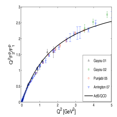
(a) (b)

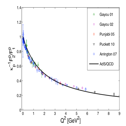
Figure 1: (Color online) AdS/QCD results are fitted with the experimental data. The plots show the ratio of Pauli and Dirac form factors for the proton, (a) the ratio is multiplied by $Q^{2}=-q^{2}=-t$, (b) the ratio is divided by $\kappa_{p}$. The experimental data are taken from Refs. Gay1 ; Gay2 ; Arr ; Pun ; Puck .

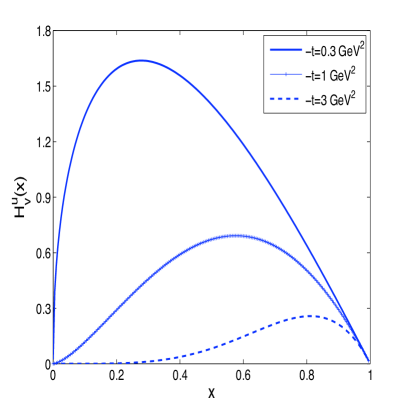
(a)  (b)

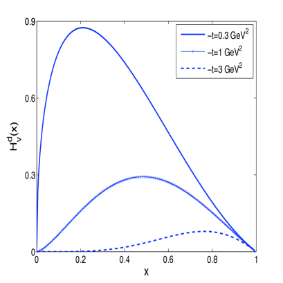
Figure 2: (Color online) Plots of (a) $H^{u}(x,t)$ vs $x$ for fixed values of $-t$ (b) the same as in (a) but for $d$ quark.

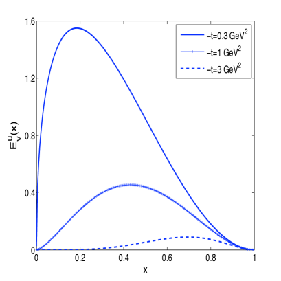
(a)  (b)

Figure 3: (Color online) Plots of (a) $E^{u}(x,t)$ vs $x$ for fixed values of $-t$; (b) $-E^{d}(x,t)$ vs $x$ for fixed values of $-t$.

In the Figs.2 (a) and (b) we show the GPD $H(x,t)$ as functions of $x$ for different $-t$ values for u and d quarks. Except for the fact that it falls off faster as $x$ increases for d quarks, the overall nature is the same for both u and d quarks. The apparent similarity in the behaviors for $u$ and $d$ quarks might be due to the $SU(6)$ symmetry in the AdS/QCD model. Similarly in Figs.3(a) and (b) we show the GPD $E(x,t)$ as a function of $x$ for different $-t$ for $u$ and $d$ quarks. Unlike $H(x,t)$, the falloff of the GPD $E(x,t)$ with increasing $x$ is similar for both $u$ and $d$ quarks.

GPDs in impact parameter space

GPDs in transverse impact parameter space are defined as burkardt :

$$H(x,b)={1\over(2\pi)^{2}}\int d^{2}\Delta e^{-i\Delta^{\perp}\cdot b^{\perp}}H(x,t),$$

$$E(x,b)={1\over(2\pi)^{2}}\int d^{2}\Delta e^{-i\Delta^{\perp}\cdot b^{\perp}}E(x,t).$$ (21)

The transverse impact parameter $b=\mid b_{\perp}\mid$ is a measure of the transverse distance between the struck parton and the center of momentum of the hadron and satisfies $\sum_{i}x_{i}b_{i}=0$, where the sum is over the number of partons. An estimate of the size of the bound state can be obtained from the relative distance between the struck parton and the center of momentum of the spectator system and is given by ${b\over 1-x}$ diehl . However, as the spatial extension of the spectator system is not available from the GPDs, exact estimation of the nuclear size is not possible. In Fig.4(a), we show the behavior of $H^{u}(x,b)$ in $x$ for fixed values of the impact parameter $b$ and in Fig.4(b) we show the same GPD as function of $b$ for fixed values of $x$, and the similar plots for $d$ quark are shown in Figs.4(c) and (d). The GPDs $E^{u/d}(x,b)$ are shown in Fig.5.

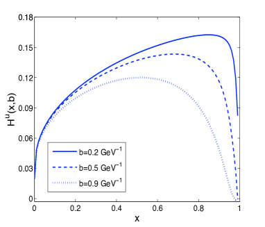
(a)  (b)

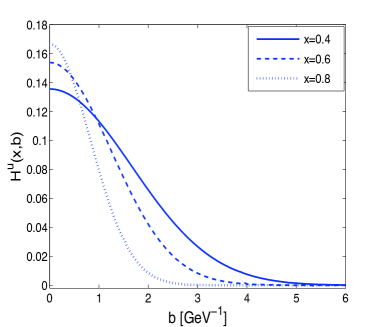
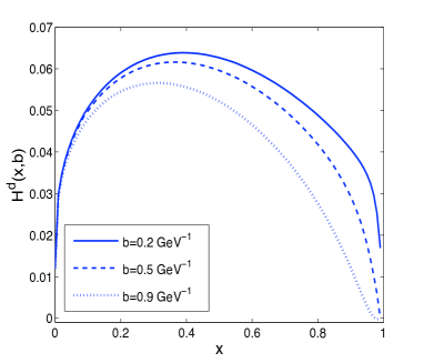
(c)  (d)

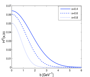
Figure 4: (Color online) Plots of (a) $H^{u}(x,b)$ vs $x$ for fixed values of impact parameter $b=\mid b_{\perp}\mid$; (b) $H^{u}(x,b)$ vs $b$ for fixed $x$; (c) and (d) are the same as in (a) and (b) but for $d$ quarks.

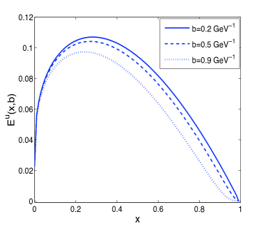
(a)  (b)

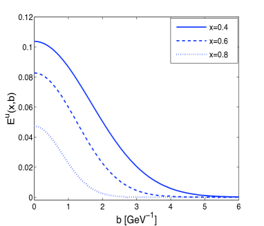
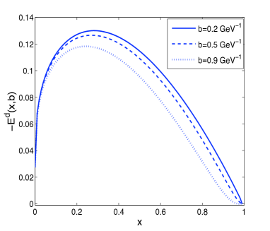
(c)  (d)

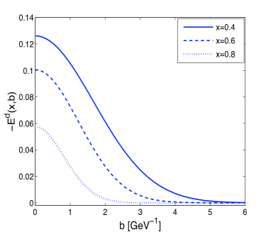
Figure 5: (Color online) Plots of (a) $E^{u}(x,b)$ vs $x$ for fixed values of $b=\mid b_{\perp}\mid$; (b) $-E^{d}(x,b)$ vs$x$ for fixed values of $b=\mid b_{\perp}\mid$ for $d$ quarks.

The GPDs evaluated in this model are qualitatively similar to the GPDs calculated in AdS/QCD using another parametrizationvega . So, it is interesting to compare with a phenomenological model. Here we compare the overall behaviors of the GPDs in the impact parameter space with those obtained from a phenomenological model for the proton proposed in Ahmed . The GPDs in this model are given by

$$H^{q}(x,t) = G^{\lambda^{q}}_{M^{q}_{x}}(x,t)x^{-\alpha^{q}-\beta^{q}_{1}(1-x)p_{1}t},$$ (22)

$$E^{q}(x,t) = \kappa_{q}G^{\lambda^{q}}_{M^{q}_{x}}(x,t)x^{-\alpha^{q}-\beta^{q}_{2}(1-x)p_{2}t},$$ (23)

where the first part is derived from the spectator model and modified by the Regge term to have proper behavior at low $x$. The parameters are fixed by fitting the form factors. The details of the functional forms and the values of the parameters can be found in Ahmed . The impact parameter dependent GPDs from this model have been studied in CMM . One should remember that the valence GPDs we have considered here in AdS/QCD are not exactly the same as GPDs in this model and so exact agreement is not expected, but it is interesting to compare and contrast the overall behaviors of the GPDs from these two models as we expect that the valence GPDs dominate the overall behavior for the GPDs in a proton.

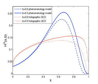
(a)  (b)

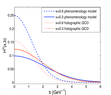
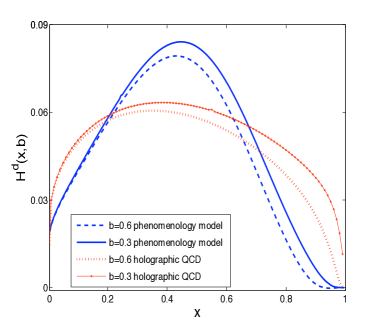
(c)  (d)

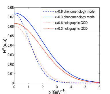
Figure 6: (Color online) Plots of (a) $H^{u}(x,b)$ vs $x$ for fixed values of impact parameter $b=\mid b_{\perp}\mid$ (b) $H^{u}(x,b)$ vs $b$ for fixed values of $x$, (c) same as in (a) but for $d$ quark and (d) same as in (b) but for $d$-quark.

In Fig.6, we compare the impact parameter dependent proton GPD $H(x,b)$ from AdS/QCD with the model mentioned above, for both $u$ and $d$ quarks. The GPDs fall off slowly for large $x$ in AdS/QCD compared to the model, while in the impact parameter space they look almost the same except for the difference in the magnitudes. In Fig.7 we have compared the two models for the proton GPD $E(x,b)$. The behavior in $x$ for $u$-quarks is quite different in the two models, while they agree better for $d$-quarks, and again the GPDs from AdS/QCD fall off slowly at large $x$ compared to the other model. In the model, the behavior of $E(x,b)$ for $u$ and $d$ quarks is quite different when plotted against $x$ for fixed values of impact parameter $b$, whereas in AdS/QCD, it shows almost the same behavior for both $u$ and $d$ quarks. The GPD $E(x,b)$ in both models agrees better in impact parameter space for the $d$-quark than the $u$-quark. The difference with the AdS/QCD results can be attributed to the fact that AdS/QCD provides only the valence wave functions in the semiclassical approximation. It is interesting to note that in both cases, at small values of impact parameter $b$, the GPD $H(x,b)$ is larger for $u$-quarks than $d$-quarks whereas the magnitude of the GPD $E(x,b)$ is marginally larger for $d$-quarks than the that for $u$-quarks. Thus it is interesting to check with other models whether this is a model independent result.

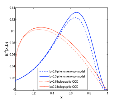
(a)  (b)

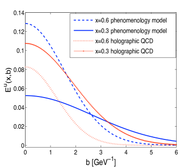
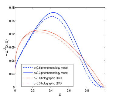
(c)  (b)

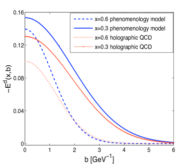
Figure 7: (Color online) Plots of (a) $E^{u}(x,b)$ vs $x$ for fixed values of $b=\mid b_{\perp}\mid$; (b) $E^{u}(x,b)$ vs. $b$ for fixed values of $x$; (c) the same as in (a) but for $d$-quarks; and (d) the same as in (b) but for $d$-quarks.

Concluding remarks
In this work we have evaluated the GPDs for protons using the LFWFs obtained from AdS/QCD. It is shown BT2 that the electromagnetic form factors for protons and neutrons calculated by using the AdS/QCD wave functions fit well with the experimental results. The GPDs are calculated using the form factors and exploiting the integral representation of the bulk-to-boundary propagator in AdS space. The valence GPDs thus obtained in the impact parameter space have been compared with the GPDs obtained from a phenomenological model. Though in the AdS/QCD we have only valence GPDs it is interesting to note that their behaviors are quite similar and agree well in impact parameter space with a phenomenological model for GPDs. But variation of the GPDs from AdS/QCD are slower than the other model when compared to the behaviors in $x$ for both $u$ and $d$ quarks.

Acknowledgements: The authors acknowledge useful discussions with Stan Brodsky and thank Stan Brodsky, Guy de Téramand and Valery Lyubovitskij for going through the previous version of the manuscript and for their valuable comments and references on the AdS/QCD and its applications.

References

- (1) For reviews on generalized parton distributions, and DVCS, see M. Diehl, Phys. Rep. 388, 41 (2003); A. V. Belitsky and A. V. Radyushkin, Phys. Rep. 418 1, (2005); K. Goeke, M. V. Polyakov, and M. Vanderhaeghen, Prog. Part. Nucl. Phys. 47, 401 (2001).
- (2) M. Burkardt, Int. J. Mod. Phys. A 18, 173 (2003).
- (3) X. Ji. Phys. Rev. Lett. 78, 610 (1997).
- (4) M. Burkardt, Phys. Rev. D 72, 094020 (2005).
- (5) C. Adloff et. al., (H1 Collaboration), Eur. Phys. J. C 13, 371 (2000).
- (6) C. Adloff et. al. (H1 Collaboration), Phys. Lett. B 517, 47 (2001).
- (7) N. D’Hose, E. Burtin, P. A. M. Guichon, J. Marroncle (COMPASS Collaboration), Eur. Phys. J. A 19, 47 (2004).
- (8) J. Breitweg et. al. (ZEUS Collaboration), Eur. Phy. J. C 6, 603 (1999).
- (9) S. Chekanov et. al. (ZEUS Collaboration), Phys. Lett. B 573, 46 (2003).
- (10) A. Airapetian et. al. (HERMES Collaboration), Phys. Rev. Lett. 87, 182001 (2001).
- (11) S. Stepanyan et. al. (CLAS Collaboration), Phys. Rev. Lett. 87, 182002 (2001).
- (12) J. Polchinski and M. J. Strassler, Phys. Rev. Lett. 88, 031601 (2002); JHEP 0305, 012 (2003).
- (13) S. J. Brodsky and G. F. de Téramond, Phys. Lett. B 582, 211 (2004), Phys. Rev. Lett. 94, 201601 (2005), Phys. Rev. Lett. 96, 201601 (2006), Phys. Rev. D 77, 056007 (2006), Phys. Rev. Lett. 102, 081601(2009).
- (14) H. Forkel, M. Beyer and T. Frederico, Int. J. Mod. Phys. E16, 2794 (2007), W. de Paula, T. Frederico, H. Forkel and M. Beyer, Phys. Rev. D 79, 75019 (2009).
- (15) A. Vega, I Schmidt, T. Branz, T. Gutsche, V. E. Lyubovitskij, Phys. Rev. D 80, 055014 (2009).
- (16) S. J. Brodsky and G. F. de Téramond, Phys. Rev. D 77, 056007 (2008); Phys. Rev. D 78, 025032 (2008), S. J. Brodsky, F-G. Cao and G. F. de Téramond, Phys. Rev. D 84, 033001(2011).
- (17) Z. Abidin and C. E. Carlson, Phys. Rev. D 79, 115003 (2009).
- (18) S. J. Brodsky and G. F. de Téramond, arXiv:1203.4025 [hep-ph].
- (19) J. R. Forshaw and R. Sandapen, Phys. Rev. Lett. 109, 081601 (2012).
- (20) M. Ahmady and R. Sandapen, Phys. Rev. D 87, 054013 (2013).
- (21) M. Ahmady and R. Sandapen, Phys. Rev. D 88, 014042 (2013).
- (22) S. D. Glazek and A. P. Trawinski, arXiv: 1307.2059 [hep-ph].
- (23) T. Gutsche, V. E. Lyubovitskij, I. Schmidt and A. Vega, Phys. Rev. D 86, 036007 (2012).
- (24) A. Vega, I. Schimdt, T. Gutsche and V. E. Lyubovitskij, Phys. Rev. D 83, 036001 (2011); Phys. Rev. D 85, 096004 (2012).
- (25) S. J. Brodsky, G. F. de Téramond, H. G. Dosch, arXiv: 1302.5399 [hep-ph].
- (26) M. Diehl, T. Feldman, R. Jacob, P. Kroll, Eur. Phys. J. C 39, 1 (2005).
- (27) H. R. Grigoryan and A. V. Radyushkin, Phys. Rev. D 76, 095007 (2007).
- (28) M. Burkardt, Int. J. Mod. Phys. A 18, 173 (2003); M. Burkardt, Phys. Rev. D 62, 071503 (2000), Erratum- ibid, D 66, 119903 (2002); J. P. Ralston and B. Pire, Phys. Rev. D 66, 111501 (2002).
- (29) S. Ahmad, H. Honkanen, S. Liuti and S. Taneja, Phys. Rev. D 75, 094003 (2007).
- (30) D. Chakrabarti, R. Manohar and A. Mukherjee, Phys. Lett. B 682, 428 (2010).
- (31) O. Gayou et. al., Phys. Rev. C 64, 038202 (2001).
- (32) O. Gayou et. al., Phys. Rev. Lett. 88, 092301 (2002).
- (33) J. Arrington, W. Melnitchouk and J. A. Tjon, Phys. Rev. C 76, 035205 (2007).
- (34) V. Punjabi et. al., Phys. Rev. C 71, 055202 (2005).
- (35) A. Puckett et. al., Phys. Rev. Lett. 104, 242301 (2010).