Large-scale Multi-label Learning with Missing Labels

Abstract

The multi-label classification problem has generated significant interest in recent years. However, existing approaches do not adequately address two key challenges: (a) the ability to tackle problems with a large number (say millions) of labels, and (b) the ability to handle data with missing labels. In this paper, we directly address both these problems by studying the multi-label problem in a generic empirical risk minimization (ERM) framework. Our framework, despite being simple, is surprisingly able to encompass several recent label-compression based methods which can be derived as special cases of our method. To optimize the ERM problem, we develop techniques that exploit the structure of specific loss functions - such as the squared loss function - to offer efficient algorithms. We further show that our learning framework admits formal excess risk bounds even in the presence of missing labels. Our risk bounds are tight and demonstrate better generalization performance for low-rank promoting trace-norm regularization when compared to (rank insensitive) Frobenius norm regularization. Finally, we present extensive empirical results on a variety of benchmark datasets and show that our methods perform significantly better than existing label compression based methods and can scale up to very large datasets such as the Wikipedia dataset.

1 Introduction

Large scale multi-label classification is an important learning problem with several applications to real-world problems such as image and video annotation Carneiro et al. (2007); Wang et al. (2009) and query/keyword suggestions Agrawal et al. (2013). The goal in multi-label classification is to accurately predict a label vector $\bm{y}\in\{0,1\}^{L}$ for a given data point $\bm{x}\in\mathbb{R}^{d}$. This problem has been studied extensively in the domain of structured output learning, where the number of labels is assumed to be small and the main focus is thus, on modeling inter-label correlations and using them to accurately predict the label vector Hariharan et al. (2010).

Due to several motivating real-life applications, recent research on multi-label classification has largely shifted its focus to the other end of the spectrum where the number of labels is assumed to be extremely large, with the key challenge being the design of scalable algorithms that offer real-time predictions and have a small memory footprint. In such situations, simple methods such as 1-vs-all or Binary Relevance (BR), that treat each label as a separate binary classification problem fail miserably. For a problem with (say) $10^{4}$ labels and $10^{6}$ features, which is common in several applications, these methods have a memory footprint of around $100$ Gigabytes and offer slow predictions.

A common technique that has been used to handle the label proliferation problem in several recent works is “label space reduction”. The key idea in this technique is to reduce the dimensionality of the label-space by using either random projections or canonical correlation analysis (CCA) based projections Chen & Lin (2012); Hsu et al. (2009); Tai & Lin (2012); Kapoor et al. (2012). Subsequently. these methods perform prediction on the smaller dimensional label-space and then recover the original labels by projecting back onto the high dimensional label-space. In particular, Chen & Lin (2012) recently showed that by using a CCA type method with appropriate orthogonality constraints, one can design an efficient algorithm with both label-space as well as feature-space compression. However, this method is relatively rigid and cannot handle several important issues inherent to multi-label problems; see Section 2.1 for more details.

In this paper we take a more direct approach by formulating the problem as that of learning a low-rank linear model $Z\in\mathbb{R}^{d\times L}$ s.t. $\bm{y}^{pred}=Z^{T}\bm{x}$. We cast this learning problem in the standard ERM framework that allows us to use a variety of loss functions and regularizations for $Z$. This framework unifies several existing dimension reduction approaches. In particular, we show that if the loss function is chosen to be the squared-$L_{2}$ loss, then our proposed formulation has a closed form solution, and surprisingly, the conditional principal label space transformation (CPLST) method of Chen & Lin (2012) can be derived as a special case. However, the flexibility of the framework allows us to use other loss functions and regularizers that are useful for preventing overfitting and increasing scalability.

Moreover, we can extend our formulation to handle missing labels; in contrast, most dimension reduction formulations (including CPLST) cannot accommodate missing labels. The ability to learn in the presence of missing labels is crucial as for most real-world applications, one cannot expect to accurately obtain (either through manual or automated labeling) all the labels for a given data point. For example, in image annotation, human labelers tag only prominent labels and typically miss out on several objects present in the image. Similarly, in online collections such as Wikipedia, where articles get tagged with categories, human labelers usually tag only with categories they know about. Moreover, there might be considerable noise/disagreement in the labeling.

In order to solve for the low-rank linear model that results from our formulation, we use the popular alternating minimization algorithm that works well despite the non-convexity of the rank constraint. For general loss functions and trace-norm regularization, we exploit subtle structures present in the problem to design a fast conjugate gradient based method. For the special case of squared-$L_{2}$ loss and trace-norm regularization, we further exploit the structure of the loss function to provide a more efficient and scalable algorithm. As compared to direct computation, our algorithm is $O(\bar{d})$ faster, where $\bar{d}$ is the average number of nonzero features in an instance.

On the theoretical side, we perform an excess risk analysis for the trace-norm regularized ERM formulation with missing labels, assuming labels are observed uniformly at random. Our proofs do not follow from existing results due to missing labels and require a careful analysis involving results from random matrix theory. Our results show that while in general the low-rank promoting trace-norm regularization does not provide better bounds than learning a full-rank matrix (e.g. using Frobenius norm regularization), for several interesting data distributions, trace-norm regularization does indeed give significantly better bounds. More specifically, for isotropic data distributions, we show that trace-norm based methods have excess risk of $O(\frac{1}{\sqrt{nL}})$ while full-rank learning can only guarantee $O(\frac{1}{\sqrt{n}})$ excess risk, where $n$ is the number of training points and $L$ is the number of labels.

Finally, we provide an extensive empirical evaluation of our method on a variety of benchmark datasets. In particular, we compare our method against three recent label compression based methods: CPLST Chen & Lin (2012), Bayesian-CS Kapoor et al. (2012), and WSABIE Weston et al. (2010). On almost all benchmark datasets, our method significantly outperforms these methods, both in the presence and absence of missing labels. Finally, we demonstrate the scalability of our method by applying it to a recently curated Wikipedia dataset Agrawal et al. (2013), that has 881,805 training samples and 213,707 labels. The results show that our method not only provides reasonably accurate solutions for such large-scale problems, but that the training time required is orders of magnitude shorter than several existing methods.

Related Work. Typically, Binary Relevance (BR), which treats each label as an independent binary classification problem, is quite accurate for multi-label classification. However, for large number of labels, this method becomes infeasible due to increased model size and prediction time. Recently, techniques have been developed that either reduce the dimensionality of the labels, such as the Compressed Sensing Approach (CS) Hsu et al. (2009), PLST Tai & Lin (2012), CPLST Chen & Lin (2012), and Bayesian CS Kapoor et al. (2012), or reduce the feature dimensionality, such as Sun et al. (2011), or both, such as WSABIE Weston et al. (2010). Most of these existing techniques are tied to a specific loss function (e.g., CPLST and BCS cater only to the squared-$L_{2}$ loss, and WSABIE works with the weighted approximate ranking loss) and/or cannot accommodate missing labels.

Our framework models multi-label classification as a general ERM problem with a low-rank constraint, which not only generalizes both label and feature dimensionality reduction but also brings in the ability to support various loss functions and allows for rigorous generalization error analysis. We show that our formulation not only retrieves CPLST, which has been shown to be fairly accurate, as a special case, but in fact substantially enhances it by use of regularization, other loss functions, allowing missing labels etc.

Paper Organization. We start by studying the generic low-rank empirical risk minimization framework for multi-label learning in Section 2. Next, we propose efficient algorithms for the framework in Section 3 and analyze the generalization performance for the trace-norm regularized ERM in Section 4. We present empirical results in Section 5, and our conclusions in Section 6.

2 Problem Formulation

In this section we present a generic ERM-style framework for multi-label classification. For each training point, we shall receive a feature vector $\bm{x}_{i}\in\mathbb{R}^{d}$ and a corresponding label vector $\bm{y}_{i}\in\left\{{0,1}\right\}^{L}$ with $L$ labels. For any $j\in[L]$, $\bm{y}_{i}^{j}=1$ will denote that the $l^{\text{th}}$ label is “present” or “on” whereas $\bm{y}_{i}^{j}=0$ will denote that the label is “absent” or “off”. Note that although we focus mostly on the binary classification setting in this paper, our methods easily extend to the multi-class setting where $\bm{y}_{i}^{j}\in\left\{{1,2,\ldots,C}\right\}$.

Our predictions for the label vector shall be parametrized as $f(\bm{x};Z)=Z^{T}\bm{x}$, where $Z\in\mathbb{R}^{d\times L}$. Although we have adopted a linear parametrization here, our results can easily be extended for non-linear kernels as well. Let $\ell(\bm{y},f(\bm{x};Z))\in\mathbb{R}$ be the loss function that computes the discrepancy between the “true” label vector and the prediction. We assume that the loss function is decomposable, i.e., $\ell(\bm{y},f(\bm{x};Z))=\sum_{j=1}^{L}\ell(\bm{y}^{j},f^{j}(\bm{x};Z))$.

The motivation for our framework comes from the observation that although the number of labels in a multi-label classification problem might be large, there typically exist significant label correlations, thus reducing the effective number of parameters required to model them to much less than $d\times L$. We capture this intuition by restricting the matrix $Z$ to learn only a small number of “latent” factors. This constrains $Z$ to be a low rank matrix which not only controls overfitting but also gives computational benefits.

Given $n$ training points our training set will be $(X,Y)$ where $X=[\bm{x}_{1},\ldots,\bm{x}_{n}]^{T}$ and $Y=[\bm{y}_{1}\ \bm{y}_{2}\ \dots\ \bm{y}_{n}]^{T}$. Using the loss function $\ell$, we propose to learn the parameters $Z$ by using the canonical regularized empirical risk minimization (ERM) method, i.e.,

$$\hat{Z}=\arg\min_{Z}J(Z) =\sum_{i=1}^{n}\sum_{j=1}^{L}\ell(Y_{ij},f^{j}(\bm{x}_{i};Z))+\lambda\cdot r(Z),$$

$$\ \ \ s.t.\ \ \mathrm{rank}(Z) \leq k,$$ (1)

where $r(Z):\mathbb{R}^{d\times L}\rightarrow\mathbb{R}$ is a regularization function. In the presence of missing labels, we compute the loss only over the known labels, i.e.,

$$\hat{Z}=\arg\min_{Z}J_{\Omega}(Z) =\sum_{(i,j)\in\Omega}\ell(Y_{ij},f^{j}(\bm{x}_{i};Z))+\lambda\cdot r(Z),$$

$$\ \ \ s.t.\ \ \mathrm{rank}(Z) \leq k,$$ (2)

where $\Omega\subseteq[n]\times[L]$ is the index set that represents “known” labels. Note that in this work, we assume the standard missing value setting, where each label can be either on, off (i.e., $Y_{ij}=1$ or $0$), or missing ($Y_{ij}=?$); several other works have considered another setting where only positive labels are known and are given as $1$ in the label matrix, while negative or missing values are all denoted by $0$ Agrawal et al. (2013); Bucak et al. (2011).

Note that although the above formulation is NP-hard in general due to the non-convex rank constraint, for convex loss functions, one can still utilize the standard alternating minimization method. Moreover, for the special case of $L_{2}$ loss, we can derive closed form solutions for the full-label case (1) and show connections to several existing methods.

We would like to note that while the ERM framework is well known and standard, most existing multi-label methods for large number of labels motivate their work in a relatively ad-hoc manner. By studying this formal framework, we can show that existing methods like CPLST Chen & Lin (2012) are in fact a special case of this generic framework (see next section). Furthermore, having this framework also helps us in studying generalization error bounds for our methods and identifying situations where the methods can be expected to succeed (see Section 4).

2.1 Special Case: Squared-$L_{2}$ loss

In this section, we study (1) and (2) for the special case of squared $L_{2}$ loss function, i.e., $\ell(\bm{y},f(\bm{x};Z))=\|\bm{y}-f(\bm{x};Z)\|_{2}^{2}$. We show that in the absence of missing labels, the formulation in (1) can be solved optimally for the squared $L_{2}$ loss using SVD. Furthermore, by selecting an appropriate regularizer $r(Z)$ and $\lambda$, our solution for $L_{2}$ loss is exactly the same as that of CPLST Chen & Lin (2012).

We first show that the unregularized form of (1) with $\ell(\bm{y},f(\bm{x};Z))=\|\bm{y}-Z^{T}\bm{x}\|_{2}^{2}$ has a closed form solution.

Claim 1.

If $\ell(\bm{y},f(\bm{x};Z))=\|\bm{y}-Z^{T}\bm{x}\|_{2}^{2}$ and $\lambda=0$, then

$$V_{X}\Sigma_{X}^{-1}M_{k}=\arg\min_{Z:\mathrm{rank}(Z)\leq k}\|Y-XZ\|_{F}^{2},$$ (3)

where $X=U_{X}\Sigma_{X}V_{X}^{T}$ is the thin SVD decomposition of $X$, and $M_{k}$ is the rank-$k$ truncated SVD of $M\equiv U_{X}^{T}Y$.

Proof of Claim 1.

Let $X=U_{X}\Sigma_{X}V_{X}^{T}$ be the thin SVD decomposition of $X$, and $M_{k}$ be the rank-$k$ truncated SVD approximation of $U_{X}^{T}Y$. We have

$$\arg\min_{Z:\mathrm{rank}(Z)\leq k}\|Y-XZ\|_{F}$$

$$= \arg\min_{Z:\mathrm{rank}(Z)\leq k}\|(U_{X}U_{X}^{T})(Y-XZ)+(I-U_{X}U_{X}^{T})(Y-XZ)\|_{F}$$

$$= \arg\min_{Z:\mathrm{rank}(Z)\leq k}\|U_{X}U_{X}^{T}(Y-XZ)\|_{F}+\|(I-U_{X}U_{X}^{T})(Y-XZ)\|_{F}$$

$$= \arg\min_{Z:\mathrm{rank}(Z)\leq k}\|U_{X}^{T}(Y-XZ)\|_{F}$$

$$= \arg\min_{Z:\mathrm{rank}(Z)\leq k}\|U_{X}^{T}Y-\Sigma_{X}V_{X}^{T}Z)\|_{F}$$

$$= V_{X}\Sigma_{X}^{-1}M_{k}\qed$$

We now show that this is exactly the solution obtained by Chen & Lin (2012) for their CPLST formulation.

Claim 2.

The solution to Equation 3 is equivalent to $Z^{\text{{CPLST}}}=W_{{CPLST}}H_{{CPLST}}^{T}$ which is the closed form solution for the CPLST scheme Chen & Lin (2012), i.e.,

$$(W_{{CPLST}},H_{{CPLST}})$$

$$= \arg\min_{\begin{subarray}{c}W\in{\mathbb{R}}^{d\times k}\\ H\in{\mathbb{R}}^{L\times k}\end{subarray}}\|XW-YH\|_{F}^{2}+\|Y-YHH^{T}\|_{F}^{2},$$

$$\quad s.t.\quad H^{T}H=I_{k}.$$ (4)

Proof of Claim 2.

Let $U_{k}[A]\Sigma_{k}[A]V_{k}[A]$ be the rank-$k$ truncated SVD approximation of a matrix $A$. In Chen & Lin (2012), the authors show that the closed form solution to (4) is

$$H_{C} =V_{k}[Y^{T}XX^{\dagger}Y],$$

$$W_{C} =X^{\dagger}YH_{C},$$

where $X^{\dagger}$ is the pseudo inverse of $X$. It follows from $X^{\dagger}=V_{X}\Sigma_{X}^{-1}U_{X}^{T}$ that $Y^{T}XX^{\dagger}Y=Y^{T}U_{X}U_{X}^{T}Y=M^{T}M$ and $V_{k}[Y^{T}XX^{\dagger}Y]=V_{k}[M].$ Thus, we have

$$Z^{CPLST} =W_{C}H_{C}^{T}$$

$$=X^{\dagger}YH_{C}H_{C}^{T}$$

$$=V_{X}^{T}\Sigma_{X}^{-1}U_{X}^{T}YV_{k}[M]V_{k}[M]^{T}$$

$$=V_{X}^{T}\Sigma_{X}^{-1}MV_{k}[M]V_{k}[M]^{T}$$

$$=V_{X}^{T}\Sigma_{X}^{-1}M_{k}\qed$$

Note that Chen & Lin (2012) derive their method by relaxing a Hamming loss problem and dropping constraints in the canonical correlation analysis in a relatively ad-hoc manner. The above results, on the other hand, show that the same model can be derived in a more principled manner. This helps us in extending the method for several other problem settings in a principled manner and also helps in providing excess risk bounds:

• As shown empirically, CPLST tends to overfit significantly whenever $d$ is large. However, we can handle this issue by setting the regularization parameter appropriately.

• The closed form solution in Chen & Lin (2012) cannot directly handle missing labels as it requires SVD on fully observed $Y$. In contrast, our framework can itself handle missing labels without any modifications.

• The formulation in Chen & Lin (2012) is tied to the $L_{2}$ loss function. In contrast, we can easily handle other loss functions; although, the optimization problem might become more difficult to solve.

3 Algorithms

In this section, we apply the alternating minimization technique for optimizing (1) and (2). For a matrix $Z$ with a known low rank $k$, it is inefficient to represent it using $d\times L$ entries, especially when $d$ and $L$ are large. Hence we consider a low-rank decomposition of the form $Z=WH^{T}$, where $W\in{\mathbb{R}}^{d\times k}$ and $H\in{\mathbb{R}}^{L\times k}$. We further assume that $r(Z)$ can be decomposed into $r_{1}(W)+r_{2}(H)$. In the following sections, we present results with the trace norm regularization, i.e., $r(Z)=\|Z\|_{\operatorname{tr}}$, which can be decomposed as $\|{Z}\|_{\operatorname{tr}}=\frac{1}{2}\left(\|W\|_{F}^{2}+\|H\|_{F}^{2}\right)$. Thus, $\min_{Z}J_{\Omega}(Z)$ under the rank constraint is equivalent to minimizing over $W,H$:

$$J_{\Omega}(W,H)=\sum_{(i,j)\in\Omega}\ell(Y_{ij},\bm{x}_{i}^{T}W\bm{h}_{j})+\frac{\lambda}{2}\left(\|W\|_{F}^{2}+\|H\|_{F}^{2}\right)$$ (5)

where $\bm{h}_{j}^{T}$ is the $j$-th row of $H$. Note that when either of $W$ or $H$ is fixed, $J_{\Omega}(W,H)$ becomes a convex function. This allows us to apply alternating minimization, a standard technique for optimizing functions with such a property, to (5). For a general loss function, after proper initialization, a sequence $\{\left(W^{(t)},H^{(t)}\right)\}$ is generated by

$$H^{(t)} \leftarrow\underset{H}{\arg\min}\quad J_{\Omega}(W^{(t-1)},H),$$

$$W^{(t)} \leftarrow\underset{W}{\arg\min}\quad J_{\Omega}(W,H^{(t)}).\vspace*{-5pt}$$

For a convex loss function, $(W^{(t)},H^{(t)})$ is guaranteed to converge to a stationary point when the minimum for both $\min_{H}J_{\Omega}\left(W^{(t-1)},H\right)$ and $\min_{W}J_{\Omega}\left(W,H^{(t)}\right)$ are uniquely defined (see Bertsekas, 1999, Proposition 2.7.1). In fact, when the squared loss is used and $Y$ is fully observed, the case considered in Section 3.2, we can prove that $(W^{(t)},H^{(t)})$ converges to the global minimum of (5) when either $\lambda=0$ or $X$ is orthogonal.

Once $W$ is fixed, updating $H$ is easy as each row $\bm{h}_{j}$ of $H$ can be independently updated as follows:

$$\bm{h}_{j}\leftarrow\underset{\bm{h}\in{\mathbb{R}}^{k}}{\arg\min}\sum_{i:(i,j)\in\Omega}\ell(Y_{ij},\bm{x}_{i}^{T}W\bm{h})+\frac{1}{2}\lambda\cdot\|\bm{h}\|_{2}^{2},$$ (6)

which is easy to solve as $k$ is small in general. Based on the choice of the loss function, (6) is essentially a linear classification or regression problem over $k$ variables with $|\{i:(i,j)\in\Omega\}|$ instances.

Algorithm 1 General Loss with Missing Labels

• To compute $\nabla g(\bm{w})$:

• $A\leftarrow XW$, where $\bm{vec}\left({W}\right)=\bm{w}$.

• $D_{ij}\leftarrow\ell^{\prime}(Y_{ij},\bm{a}_{i}^{T}\bm{h}_{j}),\ \forall(i,j)\in\Omega$.

• Return: $\bm{vec}\left({X^{T}(DH)}\right)+\lambda\bm{w}$

• To compute: $\nabla^{2}g(\bm{w})\bm{s}$

• $A\leftarrow XW$, where $\bm{vec}\left({W}\right)=\bm{w}$.

• $B\leftarrow XS$, where $\bm{vec}\left({S}\right)=\bm{s}$.

• $U_{ij}\leftarrow\ell^{\prime\prime}(Y_{ij},\bm{a}_{i}^{T}\bm{h}_{j})\bm{b}_{i}^{T}\bm{h}_{j},\ \forall(i,j)\in\Omega$.

• Return: $\bm{vec}\left({X^{T}(UH)}\right)+\lambda\bm{s}$.

Algorithm 2 Squared Loss with Full Labels

• To compute $\nabla g(\bm{w})$:

• $A\leftarrow XW$, where $\bm{vec}\left({W}\right)=\bm{w}$.

• $B\leftarrow YH$.

• $M\leftarrow H^{T}H$.

• Return: $\bm{vec}\left({X^{T}(AM-B)}\right)+\lambda\bm{w}$

• To compute: $\nabla^{2}g(\bm{w})\bm{s}$

• $A\leftarrow XS$, where $\bm{vec}\left({S}\right)=\bm{s}$.

• $M\leftarrow H^{T}H$.

• Return: $\bm{vec}\left({X^{T}(AM)}\right)+\lambda\bm{s}$

If $H$ is fixed, updating $W\in{\mathbb{R}}^{d\times k}$ is more involved as all variables are mixed up due to the pre-multiplication with $X$. Let $\tilde{\bm{x}}_{ij}=\bm{h}_{j}\otimes\bm{x}_{i}$. It is not hard to see that updating $W$ is equivalent to a regularized linear classification/regression problem with $|\Omega|$ data points $\{(Y_{ij},\tilde{\bm{x}}_{ij}):(i,j)\in\Omega\}$. Thus if $W^{*}=\arg\min_{W}\ J_{\Omega}(W,H)$ and we denote $\bm{w}^{*}:=\bm{vec}\left({W^{*}}\right)$, then $\bm{w}^{*}=\arg\min_{\bm{w}\in{\mathbb{R}}^{dk}}g(\bm{w})$,

$$g(\bm{w})\equiv\sum_{(i,j)\in\Omega}\ell\left(Y_{ij},\bm{w}^{T}\tilde{\bm{x}}_{ij}\right)+\frac{1}{2}\lambda\cdot\|\bm{w}\|_{2}^{2}.$$ (7)

Taking the squared loss as an example, the above is equivalent to a regularized least squares problem with $dk$ variables. When $d$ is large, say 1M, the closed form solution, which requires inverting a $dk\times dk$ matrix, can hardly be regarded as feasible. As a result, updating $W$ efficiently turns out to be the main challenge for alternating minimization.

In large-scale settings where both $dk$ and $|\Omega|$ are large, iterative methods such as Conjugate Gradient (CG), which perform cheap updates and offer a good approximate solution within a few iterations, are more appropriate to solve (7). Several linear classification/regression packages such as LIBLINEAR Fan et al. (2008) can handle such problems if $\{\tilde{\bm{x}}_{ij}:(i,j)\in\Omega\}$ are available. The main operation in such iterative methods is a gradient calculation ($\nabla g(\bm{w})$) or a multiplication of the Hessian matrix and a vector ($\nabla^{2}g(\bm{w})\bm{s}$). Let $\tilde{X}=[\cdots\tilde{\bm{x}}_{ij}\cdots]^{T}_{(i,j)\in\Omega}$ and $\bar{d}=\sum_{i=1}^{n}\|\bm{x}\|_{0}/n$. Then these operations require at least $nnz(\tilde{X})=O(|\Omega|\bar{d}k)$ time to compute in general.

However, as we show below, we can exploit the structure in $\tilde{X}$ to develop efficient techniques such that both the operations mentioned above can be done in $O\left(\left(|\Omega|+nnz(X)+d+L\right)\times k\right)$ time. As a result, iterative methods, such as CG, can achieve $O(\bar{d})$ speedup. See Appendix A.1 for a detailed CG procedure for (7) with the squared loss. Our techniques, thus, make the alternating minimization method efficient enough to handle large-scale problems.

3.1 Fast Operations for General Loss Functions with Missing Labels

We assume that the loss function is a general twice-differentiable function $\ell(a,b),$ where $a$ and $b$ are scalars. Let $\ell^{\prime}(a,b)=\frac{\partial}{\partial b}\ell(a,b)$, and $\ell^{\prime\prime}(a,b)=\frac{\partial^{2}}{\partial b^{2}}\ell(a,b)$. The gradient and the Hessian matrix for $g(\bm{w})$ are:

$$\nabla g(\bm{w}) =\sum_{(i,j)\in\Omega}\ell^{\prime}(Y_{ij},\bm{w}^{T}\tilde{\bm{x}}_{ij})\tilde{\bm{x}}_{ij}+\lambda\bm{w},$$ (8)

$$\nabla^{2}g(\bm{w}) =\sum_{(i,j)\in\Omega}\ell^{\prime\prime}(Y_{ij},\bm{w}^{T}\tilde{\bm{x}}_{ij})\tilde{\bm{x}}_{ij}\tilde{\bm{x}}_{ij}^{T}+\lambda I.\vspace*{-5pt}$$ (9)

A direct computation of $\nabla g(\bm{w})$ and $\nabla^{2}g(\bm{w})\bm{s}$ using (8) and (9) requires at least $O(|\Omega|\bar{d}k)$ time. Below we give faster procedures to perform both operations.

Gradient Calculation. Recall that $\tilde{\bm{x}}_{ij}=\bm{h}_{j}\otimes\bm{x}_{i}=\bm{vec}\left({\bm{x}_{i}\bm{h}_{j}^{T}}\right)$. Therefore, we have

$$\sum_{(i,j)\in\Omega}\ell^{\prime}(Y_{ij},\bm{w}^{T}\tilde{\bm{x}}_{ij})\bm{x}_{i}\bm{h}_{j}^{T}=X^{T}DH,$$

where $D$ is sparse with $D_{ij}=\ell^{\prime}(Y_{ij},\bm{w}^{T}\tilde{\bm{x}}_{ij}),\ \forall(i,j)\in\Omega$. Thus,

$$\nabla g(\bm{w})=\bm{vec}\left({X^{T}DH}\right)+\lambda\bm{w}.$$ (10)

Assuming that $\ell^{\prime}(a,b)$ can be computed in constant time, which holds for most loss functions (e.g. squared-$L_{2}$ loss, logistic loss), the gradient computation can be done in $O\left(\left(nnz(X)+|\Omega|+d\right)\times k\right)$ time. Algorithm 1 gives the details of computing $\nabla g(\bm{w})$ using (10).

Hessian-vector Multiplication. After substituting $\tilde{\bm{x}}_{ij}=\bm{h}_{j}\otimes\bm{x}_{i}$, we have

$$\nabla^{2}g(\bm{w})\bm{s}=\sum_{(i,j)\in\Omega}\ell^{\prime\prime}_{ij}\cdot\left((\bm{h}_{j}\bm{h}_{j}^{T})\otimes(\bm{x}_{i}\bm{x}_{i}^{T})\right)\bm{s}+\lambda\bm{s},$$

where $\ell^{\prime\prime}_{ij}=\ell^{\prime\prime}(Y_{ij},\bm{w}^{T}\tilde{\bm{x}}_{ij})$. Let $S$ be the $d\times k$ matrix such that $\bm{s}=\bm{vec}\left({S}\right)$. Using the identity $(B^{T}\otimes A)\bm{vec}\left({X}\right)=\bm{vec}\left({AXB}\right)$, we have $\left((\bm{h}_{j}\bm{h}_{j}^{T})\otimes(\bm{x}_{i}\bm{x}_{i}^{T})\right)\bm{s}=\bm{vec}\left({\bm{x}_{i}\bm{x}_{i}^{T}S\bm{h}_{j}\bm{h}_{j}^{T}}\right)$. Thus,

$$\sum_{ij}\ell^{\prime\prime}_{ij}\bm{x}_{i}\bm{x}_{i}^{T}S\bm{h}_{j}\bm{h}_{j}^{T} =\sum_{i=1}^{n}\bm{x}_{i}(\sum_{j:(i,j)\in\Omega}\ell^{\prime\prime}_{ij}\cdot(S^{T}\bm{x}_{i})^{T}\bm{h}_{j}\bm{h}_{j}^{T})$$

$$=\sum_{i=1}^{n}\bm{x}_{i}(\sum_{j:(i,j)\in\Omega}U_{ij}\bm{h}_{j}^{T})=X^{T}UH,$$

where $U$ is sparse, and $U_{ij}~{}=\ell^{\prime\prime}_{ij}\cdot(S^{T}\bm{x}_{i})^{T}\bm{h}_{j},\ \forall(i,j)\in\Omega$. Thus, we have

$$\nabla^{2}g(\bm{w})\bm{s}=\bm{vec}\left({X^{T}UH}\right)+\lambda\bm{s}.$$ (11)

In Algorithm 1, we describe a detailed procedure for computing the Hessian-vector multiplication in $O\left(\left(nnz(X)+|\Omega|+d\right)\times k\right)$ time using (11).

Table 1: Computation of $\ell^{\prime}(a,b)$ and $\ell^{\prime\prime}(a,b)$ for different loss functions. Note that for the logistic and $L_{2}$-hinge loss in Table 1, $Y_{ij}$ is assumed to be ${-1,+1}$ instead of $\{0,1\}$.

	$\ell(a,b)$	$\frac{\partial}{\partial b}\ell(a,b)$	$\frac{\partial^{2}}{\partial b^{2}}\ell(a,b)$
Squared loss	$\frac{1}{2}(a-b)^{2}$	$b-a$	$1$
Logistic loss	$\log\left(1+e^{-ab}\right)$	$\frac{-a}{1+e^{-ab}}$	$\frac{-a^{2}e^{-ab}}{\left(1+e^{-ab}\right)^{2}}$
$L_{2}$-hinge loss	$\left(\max(0,1-ab)\right)^{2}$	$-2a\max(0,1-ab)$	$2\cdot{\mathcal{I}}[ab<1]$

Loss Functions. See Table 1 for expressions of $\ell^{\prime}(a,b)$ and $\ell^{\prime\prime}(a,b)$ for three common loss functions: squared loss, logistic loss, and squared hinge loss. Thus, to solve (7), we can apply CG for squared loss and the trust region Newton method (TRON) Lin et al. (2008) for the other two loss functions.

3.2 Fast Operations for Squared Loss with Full Labels

For the situation where labels are fully observed, solving (1) efficiently in the large-scale setting remains a challenge. The closed form solution from (3) is not ideal for two reasons: firstly since it involves the SVD of both $X$ and $U_{X}^{T}Y$, the solution becomes infeasible when rank of $X$ is large. Secondly, since it is an unregularized solution, it might overfit. Indeed CPLST has similar scalability and overfitting issues due to absence of regularization and requirement of pseudo inverse calculations for $X$. When $Y$ is fully observed, Algorithm 1, which aims to handle missing labels with a general loss function, is also not scalable as $|\Omega|=nL$ imposing a $O\left(nLk+nnz(X)k\right)$ cost per operation which is prohibitive when $n$ and $L$ are large.

Although, for a general loss, an $O(nLk)$ cost seems to be inevitable, for the $L_{2}$ loss, we propose fast procedures such that the cost of each operation only depends on $nnz(Y)$ instead of $|\Omega|$. In most real-world multi-label problems, $nnz(Y)\ll nL=|\Omega|$. As a result, for the squared loss, our technique allows alternating minimization to be performed efficiently even when $|\Omega|=nL$.

If the squared loss is used, the matrix $D$ in Eq. (10) is $D=XWH^{T}-Y$ when $Y$ is fully observed, where $W$ is the $d\times k$ matrix such that $\bm{vec}\left({W}\right)=\bm{w}$. Then, we have

$$\nabla g(\bm{w})=\bm{vec}\left({X^{T}XWH^{T}H-X^{T}YH}\right)+\lambda\bm{w}.$$ (12)

Similarly, $U$ in Eq. (11) is $U=XSH^{T}$ which gives us

$$\nabla^{2}g(\bm{w})\bm{s}=\bm{vec}\left({X^{T}XSH^{T}H}\right)+\lambda\bm{s}.$$ (13)

With a careful choice of the sequence of the matrix multiplications, we show detailed procedures in Algorithm 2, which use only $O(nk+k^{2})$ extra space and $O\left(\left(nnz(Y)+nnz(X)\right)k+(n+L)k^{2}\right)$ time to compute both $\nabla g(\bm{w})$ and $\nabla^{2}g(\bm{w})\bm{s}$ efficiently.

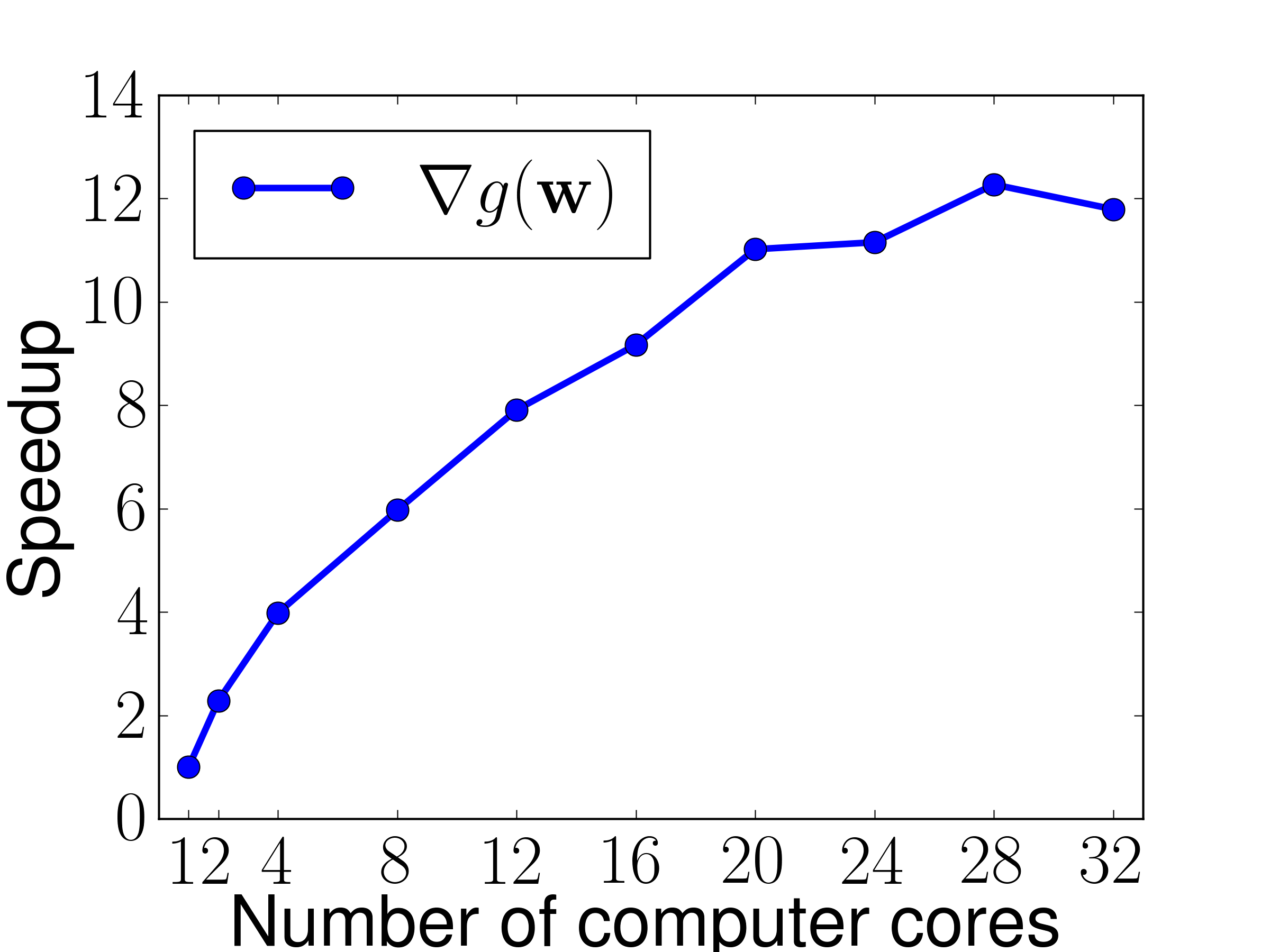
(a) $\nabla g(\bm{w})$

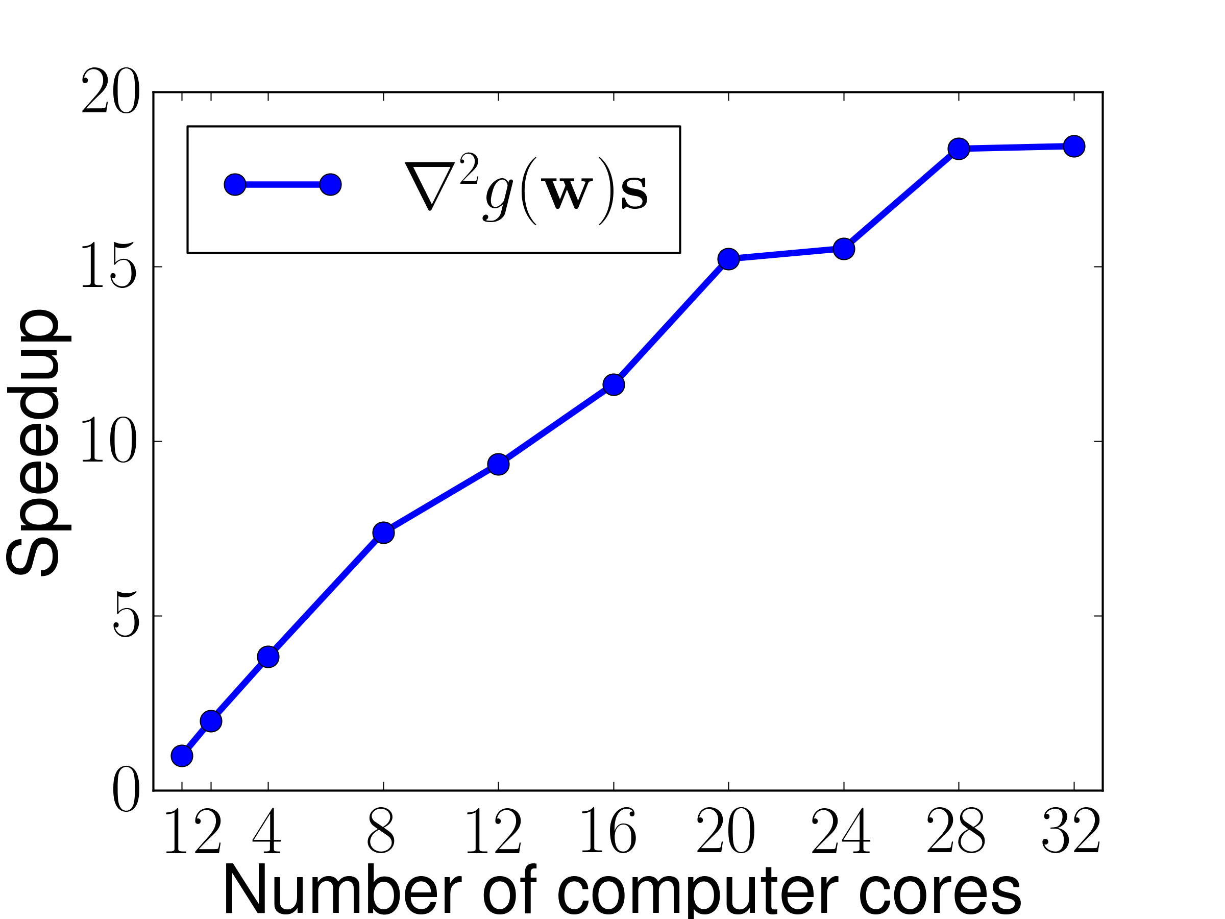
(b) $\nabla^{2}g(\bm{w})\bm{s}$

Figure 3: Speedup results for our proposed fast gradient calculation and Hessian-vector multiplication.

Remark on parallelization. As we can see, matrix multiplication acts as a crucial subroutine in both Algorithms 1 and 2. Thus, with a highly-optimized parallel BLAS library (such as ATLAS or Intel MKL), our algorithms can easily enjoy speedup brought by the parallel matrix operations provided in the library without any extra efforts. Figure 3 in Appendix D shows that both algorithms do indeed enjoy impressive speedups as the number of cores increases.

Remark on kernel extension. Given a kernel function ${\mathcal{K}}(\cdot,\cdot)$, let $f^{j}\in{\mathcal{H}}_{{\mathcal{K}}}$ be the minimizer of the empirical loss defined in Eq. (2). Then by the Representer Theorem (for example, Schölkopf et al., 2001), $f^{j}$ admits a representation of the form: $f^{j}(\cdot;\bm{z}_{j})=\sum_{t=1}^{n}z_{jt}{\mathcal{K}}(\cdot,\bm{x}_{t}),$ where $\bm{z}_{j}\in{\mathbb{R}}^{n}$. Let the vector function $\bm{k}(\bm{x}):{\mathbb{R}}^{d}\rightarrow{\mathbb{R}}^{n}$ for ${\mathcal{K}}$ be defined as $\bm{k}(\bm{x})=[\cdots,{\mathcal{K}}(\bm{x},\bm{x}_{t}),\cdots]^{T}$. Then $f(\bm{x};Z)$ can be written as $f(\bm{x};Z)=Z^{T}\bm{k}(\bm{x})$, where $Z$ is an $n\times L$ matrix with $\bm{z}_{j}$ as the $j$-th column. Once again, we can impose the same trace norm regularization $r(Z)$ and the low rank constraint in Eq. (5). As a result, $Z=WH^{T}$ and $f^{j}(\bm{x}_{i},\bm{z}_{j})=\bm{k}^{T}(\bm{x}_{i})W\bm{h}_{j}$. If $K$ is the kernel Gram matrix for the training set $\{\bm{x}_{i}:i=1,\ldots,n\}$ and $K_{i}$ is its $i^{\text{th}}$ column, then the loss in (5) can be replaced by $\l(Y_{ij},K_{i}^{T}W\bm{h}_{j})$. Thus, the proposed alternating minimization can be applied to solve Equations (1) and (2) with the kernel extension as well.

4 Generalization Error Bounds

In this section we analyze excess risk bounds for our learning model with trace norm regularization. Our analysis demonstrates the superiority of our trace norm regularization-based technique over BR and Frobenius norm regularization. We require a more careful analysis for our setting since standard results do not apply because of the presence of missing labels.

Our multi-label learning model is characterized by a distribution ${{\cal D}}$ on the space of data points and labels ${\cal X}\times\left\{{0,1}\right\}^{L}$ where ${\cal X}\subseteq\mathbb{R}^{d}$ and a distribution that decides the pattern of missing labels. We receive $n$ training points $(\bm{x}_{1},\bm{y}_{1}),\ldots,(\bm{x}_{n},\bm{y}_{n})$ sampled i.i.d from the distribution ${{\cal D}}$, where $\bm{y}_{i}\in\left\{{0,1}\right\}^{L}$ are the ground truth label vectors. However we shall only be able to observe the ground truth label vectors $\bm{y}_{i}$ at $s$ random locations. More specifically, for each $i$ we only observe $\bm{y}_{i}$ at locations $l_{i}^{1},\ldots,l_{i}^{s}\in[L]$ where the locations are chosen uniformly from the set $[L]$ and the choices are independent of $(\bm{x}_{i},\bm{y}_{i})$.

Given this training data, we learn a predictor $\hat{Z}$ by performing empirical risk minimization over a constrained set of predictors as follows:

$$\hat{Z}=\underset{r(Z)\leq\lambda}{\arg\inf}\ \hat{\cal L}(Z)=\frac{1}{n}\sum_{i=1}^{n}\sum_{j=1}^{s}\ell(\bm{y}_{i}^{l_{i}^{j}},f^{l_{i}^{j}}(\bm{x}_{i};Z)),$$

where $\hat{\cal L}(Z)$ is the empirical risk of a predictor $Z$. Note that although the method in Equation 2 uses a regularized formulation that is rank-constrained, we analyze just the regularized version without the rank constraints for simplicity. As the class of rank-constrained matrices is smaller than the class of trace-norm constrained matrices, we can in fact expect better generalization performance than that indicated here, if the ERM problem can be solved exactly.

Our goal would be to show that $\hat{Z}$ has good generalization properties i.e. ${\cal L}(\hat{Z})\leq\underset{r(Z)\leq\lambda}{\inf}{\cal L}(Z)+\epsilon,$ where ${\cal L}(Z):=\underset{\bm{x},\bm{y},l}{\mathbb{E}}\left\llbracket{{\ell(\bm{y}^{l},f^{l}(\bm{x};Z))}}\right\rrbracket$ is the population risk of a predictor.

Theorem 3.

Suppose we learn a predictor using the formulation $\hat{Z}=\underset{\left\|{Z}\right\|_{\operatorname{tr}}\leq\lambda}{\arg\inf}\ \hat{\cal L}(Z)$ over a set of $n$ training points. Then with probability at least $1-\delta$, we have

$${\cal L}(\hat{Z})\leq\underset{\left\|{Z}\right\|_{\operatorname{tr}}\leq\lambda}{\arg\inf}\ {\cal L}(Z)+{\cal O}\left({{s\lambda\sqrt{\frac{1}{n}}}}\right)+{\cal O}\left({{s\sqrt{\frac{\log\frac{1}{\delta}}{{n}}}}}\right),$$

where we assume (w.l.o.g.) that $\mathbb{E}\left\llbracket{\left\|{\bm{x}}\right\|_{2}^{2}}\right\rrbracket\leq 1$.

We refer to Appendix B for the proof. Interestingly, we can show that our analysis, obtained via uniform convergence bounds, is tight and cannot be improved in general. We refer the reader to Appendix C.1 for the tightness argument. However, it turns out that Frobenius norm regularization is also able to offer the same excess risk bounds and thus, this result does not reveal any advantage for trace norm regularization. Nevertheless, we can still get improved bounds for a general class of distributions over $(\bm{x},\bm{y})$:

Theorem 4.

Let the data distribution satisfy the following conditions: 1) The top singular value of the covariance matrix $X=\underset{\bm{x}\sim{{\cal D}}}{\mathbb{E}}\left\llbracket{{\bm{x}\bm{x}^{\top}}}\right\rrbracket$ is $\|X\|_{2}=\sigma_{1}$, 2) $\text{tr}\left({X}\right)=\Sigma$ and 3) the distribution on ${\cal X}$ is sub-Gaussian i.e. for some $\eta>0$, for all $\bm{v}\in\mathbb{R}^{d}$, $\mathbb{E}\left\llbracket{\exp\left(x^{\top}\bm{v}\right)}\right\rrbracket\leq\exp\left(\left\|{\bm{v}}\right\|_{2}^{2}\eta^{2}/2\right)$, then with probability at least $1-\delta$, we have

$${\cal L}(\hat{Z})\leq\underset{\left\|{Z}\right\|_{\operatorname{tr}}\leq\lambda}{\arg\inf}\ {\cal L}(Z)+{\cal O}\left({{s\lambda\sqrt{\frac{d(\eta^{2}+\sigma_{1})}{nL\Sigma}}+s\sqrt{\frac{\log\frac{1}{\delta}}{{n}}}}}\right).$$

In particular, if the data points are generated from a unit normal distribution, then we have

$${\cal L}(\hat{Z})\leq\underset{\left\|{Z}\right\|_{\operatorname{tr}}\leq\lambda}{\arg\inf}\ {\cal L}(Z)+{\cal O}\left({{s\lambda\sqrt{\frac{1}{nL}}}}\right)+{\cal O}\left({{s\sqrt{\frac{\log\frac{1}{\delta}}{{n}}}}}\right).$$

The proof of Theorem 4 can be found in Appendix B. Our proofs do not follow either from existing techniques for learning with matrix predictors (for instance Kakade et al. (2012)) or from results on matrix completion with trace norm regularization Shamir & Shalev-Shwartz (2011) due to the complex interplay of feature vectors and missing labels that we encounter in our learning model. Instead, our results utilize a novel form of Rademacher averages, bounding which requires tools from random matrix theory. We note that our results can even handle non-uniform sampling of labels (see Theorem 6 in Appendix B for details).

We note that the assumptions on the data distribution are trivially satisfied with finite $\sigma_{1}$ and $\eta$ by any distribution with support over a compact set. However, for certain distributions, this allows us to give superior bounds for trace norm regularization. We note that Frobenius norm regularization can give no better than a $\left({\frac{\lambda}{\sqrt{n}}}\right)$ style excess error bound even for such distributions (see Appendix C.2 for a proof), whereas trace norm regularization allows us to get superior $\left({\frac{\lambda}{\sqrt{nL}}}\right)$ style bounds. This is especially contrasting when, for instance, $\lambda={\cal O}(\sqrt{L})$, in which case trace norm regularization gives ${\cal O}\left({{\frac{1}{\sqrt{n}}}}\right)$ excess error whereas the excess error for Frobenius regularization deteriorates to ${\cal O}\left({{\sqrt{\frac{L}{n}}}}\right)$. Thus, trace norm seems better suited to exploit situations where the data distribution is isotropic.

Intuitively, we expect such results due to the following reason: when labels are very sparsely observed, such as when $s={\cal O}\left({{1}}\right)$, we observe the value of each label on ${\cal O}\left({{n/L}}\right)$ training points. In such a situation, Frobenius norm regularization with say $\lambda=\sqrt{L}$ essentially allows an independent predictor $z_{l}\in\mathbb{R}^{d}$ to be learned for each label $l\in[L]$. Since all these predictors are being trained on only ${\cal O}\left({{n/L}}\right)$ training points, the performance accordingly suffers.

On the other hand, if we were to train a single predictor for all the labels i.e. $Z=z\bm{1}^{\top}$ for some $z\in\mathbb{R}^{d}$, such a predictor would be able to observe $O(n)$ points and consequently have much better generalization properties. Note that this predictor also satisfies $\|z\bm{1}^{\top}\|_{\operatorname{tr}}\leq\sqrt{L}$. This seems to indicate that trace norm regularization can capture cross label dependencies, especially in the presence of missing labels, much better than Frobenius norm regularization.

Having said that, it is important to note that the two regularizations (trace norm vs. Frobenius norm) might induce different biases in the learning framework. It would be an interesting exercise to study the bias-variance trade-offs offered by these two regularization techniques. However, if one has label correlations then we expect both formulations to suffer similar biases.

5 Experimental Results

Table 2: Data statistics. $d$ and $L$ are the number of features and labels, respectively, and $\bar{d}$ and $\bar{L}$ are the average number of nonzero features and positive labels in an instance, respectively.

			Training set			Test set
Dataset	$d$	$L$	$n$	$\bar{d}$	$\bar{L}$	$n$	$\bar{d}$	$\bar{L}$
bibtex	1,836	159	4,880	68.74	2.40	2,515	68.50	2.40
autofood	9,382	162	155	143.92	15.80	38	143.71	13.71
compphys	33,284	208	161	792.78	9.80	40	899.02	11.83
delicious	500	983	12,920	18.17	19.03	3,185	18.80	19.00
eurlex	5,000	3,993	17,413	236.69	5.30	1,935	240.96	5.32
nus-wide	1,134	1,000	161,789	862.70	5.78	107,859	862.94	5.79
wiki	366,932	213,707	881,805	146.78	7.06	10,000	147.78	7.08

We now present experimental results in order to assess our proposed algorithms in terms of accuracy and scalability. As we shall see, the results unambiguously demonstrate the superiority of our method over other approaches.

Datasets. We consider a variety of benchmark datasets including four standard datasets (bibtex, delicious, eurlex, and nus-wide), two datasets with $d\gg L$ (autofood and compphys), and a very large scale Wikipedia based dataset, which contains about 1M wikipages and 200K labels. See Table 2 for more information about the datasets. We conducted all experiments on an Intel machine with 32 cores.

Table 3: Comparison of LEML with various loss functions and WSABIE on smaller datasets. SQ denotes squared loss, LR denotes logistic regression loss, and SH denotes squared hinge loss

		Top-$3$ Accuracy				Average AUC
		LEML			WSABIE	LEML			WSABIE
	$k/L$	SQ	LR	SH		SQ	LR	SH
bibtex	$20\%$	34.16	25.65	27.37	28.77	0.8910	0.8677	0.8541	0.9055
	$40\%$	36.53	28.20	24.81	30.05	0.9015	0.8809	0.8467	0.9092
	$60\%$	38.00	28.68	23.26	31.11	0.9040	0.8861	0.8505	0.9089
autofood	$20\%$	81.58	80.70	81.58	66.67	0.9565	0.9598	0.9424	0.8779
	$40\%$	76.32	80.70	78.95	70.18	0.9277	0.9590	0.9485	0.8806
	$60\%$	70.18	80.70	81.58	60.53	0.8815	0.9582	0.9513	0.8518
compphys	$20\%$	80.00	80.00	80.00	49.17	0.9163	0.9223	0.9274	0.8212
	$40\%$	80.00	78.33	79.17	39.17	0.9199	0.9157	0.9191	0.8066
	$60\%$	80.00	80.00	80.00	49.17	0.9179	0.9143	0.9098	0.8040
delicious	$20\%$	61.20	53.68	57.27	42.87	0.8854	0.8588	0.8894	0.8561
	$40\%$	61.23	49.13	52.95	42.05	0.8827	0.8534	0.8868	0.8553
	$60\%$	61.15	46.76	49.58	42.22	0.8814	0.8517	0.8852	0.8523

Table 4: Comparison of LEML and WSABIE on large datasets

		LEML				WSABIE
dataset	$k$	time (s)	top-$1$	top-$3$	AUC	time (s)	top-$1$	top-$3$	AUC
eurlex	250	175	51.99	39.79	0.9425	373	33.13	25.01	0.8648
	500	487	56.90	44.20	0.9456	777	31.58	24.00	0.8651
nus-wide	50	574	20.71	15.96	0.7741	4,705	14.58	11.37	0.7658
	100	1,097	20.76	16.00	0.7718	6,880	12.46	10.21	0.7597
wiki	250	9,932	19.56	14.43	0.9086	79,086	18.91	14.65	0.9020
	500	18,072	22.83	17.30	0.9374	139,290	19.20	15.66	0.9058

Competing Methods. A list containing details of the competing methods (including ours) is given below. Note that CS Hsu et al. (2009) and PLST Tai & Lin (2012) are not included as they are shown to be suboptimal to CPLST and BCS in Chen & Lin (2012); Kapoor et al. (2012).

• LEML (Low rank Empirical risk minimization for Multi-Label Learning): our proposed method. We implemented CG with Algorithms 1 and 2 for squared loss, and TRON Lin et al. (2008) with Algorithm 1 for logistic and squared hinge loss.

• CPLST: the method proposed in Chen & Lin (2012). We used the code provided by the author.

• BCS: the Bayesian compressed sensing method of Kapoor et al. (2012). We used code provided by the authors to test this method.

• BR: Binary Relevance with various loss functions.

• WSABIE: As there is no publicly available code, we implemented this method and hand-tuned the learning rate and the margin for each dataset as suggested by the authors of WSABIE (Weston, 2013).
  

Evaluation Criteria. Three criteria will be used to compare the methods: top-K accuracy, which measures the performance on a few top predictions, Hamming loss, which considers the overall classification performance, and average AUC, which takes the overall ranking into account.

Given a test set $\{\bm{x}_{i},\bm{y}_{i}:i=1,\ldots,n\}$ and an real-valued predictor $f(\bm{x}):\mathbb{R}^{d}\rightarrow\mathbb{R}$:

• Top-$K$ accuracy: for each instance, we select the $K$ labels with the largest decision values for prediction. The average accuracy among all instances are reported as the top-$K$ accuracy.

• Hamming-loss: for each pair of instance $\bm{x}$ and label index $j$, we round the decision value $f^{j}(\bm{x})$ to 0 or 1.

  $$\text{Hamming Loss}=\frac{1}{nL}\sum_{i=1}^{n}\sum_{j=1}^{L}I[\text{round}\left(f^{j}(\bm{x})\right)\neq\bm{y}^{j}]$$

• Average AUC: we follow Bucak et al. (2009) to calculate area under ROC curve for each instance and report the average AUC among all test instances.

5.1 Results with full labels

We divide datasets into two groups: small datasets (bibtex, autofood, compphys, and delicious) on which BCS and CPLST can be tested without scalability issues and large datasets (eurlex, nus-wide, and wiki) to which only LEML and WSABIE are able to scale.

Small datasets. We first compare dimension reduction based approaches to assess their performance with varying dimensionality reduction ratios. Figure 1 presents these results for LEML, CPLST and BCS on the squared $L_{2}$ loss with BR included for reference. Clearly LEML consistently performs better than other methods for all ratios. Next we compare LEML with three loss functions (squared, logistic, and $L_{2}$-hinge) to WSABIE, which approximately optimizes a weighted approximate ranking loss. As Table 3 shows, although the best loss for each dataset might vary, LEML is always superior to or competitive with WSABIE. Based on Figure 1, Table 3, and further results in Appendix D.2, we make the following observations. 1) LEML can deliver accuracies competitive with BR even with a severe reduction in dimensionality, 2) On bibtex and compphys, LEML is even shown to outperform BR. This is a benefit brought forward by the design of LEML, wherein the relation between labels can be captured by a low rank $Z$. This enables LEML to better utilize label information than BR and yield better accuracies. 3) On autofood and compphys, CPLST seems to suffer from overfitting and demonstrates a significant dip in performance. In contrast, LEML, which brings regularization into the formulation performs well consistently on all datasets.

Larger data. Table 4 shows results for LEML and WSABIE on the three larger datasets. We implemented LEML with the squared $L_{2}$ loss using Algorithm 2 for comparison in the full labels case. Note that Hamming loss is not used here as it is not clear how to convert the label ranking given by WSABIE to a 0/1 encoding. For LEML, we report the time and the accuracies obtained after five alternating iterations. For WSABIE, we ran the method on each dataset with the hand-tuned parameters for about two days, and reported the time and results for the epoch with the highest average AUC. On eurlex and nus-wide, LEML is clearly superior than WSABIE on all evaluation criteria. On wiki, although both methods share a similar performance for $k=250$, on increasing $k$ to $500$, LEML again outperforms WSABIE. Also clearly noticeable is the stark difference in the running times of the two methods. Whereas LEML takes less than 6 hours to deliver 0.9374 AUC on wiki, WSABIE requires about 1.6 days to achieve 0.9058 AUC. More specifically, WSABIE takes about 7,000s for the first epoch, 16,000s for the second and 36,000s for the third epoch which result in it spending almost two days on just 5 epochs. Although this phenomenon is expected due to the sampling scheme in WSABIE Weston et al. (2010), it becomes more serious as $L$ increases. We leave the issue of designing a better sampling scheme with large $L$ for future work. Figure 2a further illustrates this gap in training times for the nus-wide dataset. All in all, the results clearly demonstrate the scalability and efficiency of LEML.

Table 5: Comparison between various dimensionality reduction approaches on $Y$ with 20% observed entries, and $k=0.4L$.

	Top-$3$ Accuracy			Hamming loss			Average AUC
	LEML	BCS	BR	LEML	BCS	BR	LEML	BCS	BR
bibtex	28.50	23.84	25.78	0.0136	0.2496	0.0193	0.8332	0.7871	0.8087
autofood	67.54	35.09	62.28	0.0671	0.2445	0.0760	0.8634	0.6322	0.8178
compphys	65.00	35.83	31.67	0.0518	0.2569	0.0566	0.7964	0.6442	0.7459

5.2 Results with missing labels

For experiments with missing labels, we compare LEML, BCS, and BR. We implemented BR with missing labels by learning an $L_{2}$-regularized binary classifier/regressor for each label on observed instances. Thus, the model derived from BR corresponds to the minimizer of (2) with Frobenius norm regularization. Table 5 shows the results when $20\%$ entries were revealed (i.e. $80\%$ missing rate) and squared loss function was used for training. We used $k=0.4L$ for both LEML and BCS. The results clearly show that LEML outperforms BCS and LEML with respect to all three evaluation criteria. On bibtex, we further present results for various rates of observed labels in Figure 2b and results for various dimension reduction ratios in Figure 2c. LEML clearly shows superior performance over other approaches, which corroborates the theoretical results of Section 4 that indicate better generalization performance for low-rank promoting regularizations. More empirical results for other loss functions, various observed ratios and dimension reduction ratios can be found in Appendix D.3.

(a) bibtex

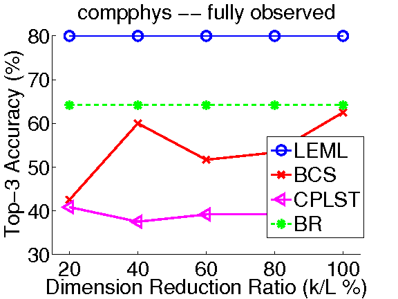
(b) compphys

(c) delicious

Figure 1: Comparison between different dimensionality reduction methods with fully observed $Y$ by varying the ratio of dimension reduction $k/L$.

(a)

(b)

(c)

Figure 2: Results for (a): LEML vs. WSABIE on nus-wide. (b): bibtex with various observed ratios. (c): bibtex with various ratios of dimension reduction.

6 Conclusion

In this paper we studied the multi-label learning problem with missing labels in the standard ERM framework. We modeled our framework with rank constraints and regularizers to increase scalability and efficiency. To solve the obtained non-convex problem, we proposed an alternating minimization based method that critically exploits structure in the loss function to make our method scalable. We showed that our learning framework admits excess risk bounds that indicate better generalization performance for our methods than the existing methods like BR, something which our experiments also confirmed. Our experiments additionally demonstrated that our techniques are much more efficient than other large scale multi-label classifiers and give superior performance than the existing label compression based approaches. For future work, we would like to extend LEML to other (non decomposable) loss functions such as ranking losses and study conditions under which alternating minimization for our problem is guaranteed to converge to the global optimum. Another open question is if our risk bounds can be improved by avoiding the uniform convergence route that we use in the paper.

Appendix A Algorithm Details

A.1 Conjugate Gradient for Squared Loss

In Algorithm 3, we show the detailed conjugate gradient procedure used to solve (7) when the squared loss is used. Note that $\nabla^{2}g(\bm{w})$ is invariant to $\bm{w}$ as (7) is a quadratic problem due to the squared loss function.

Algorithm 3 Conjugate gradient for solving (7) with the squared loss

• Set initial $\bm{w}_{0}$, $\bm{r}_{0}=-\nabla g(\bm{w}_{0})$, $\bm{d}_{0}=\bm{r}_{0}$.

• For $t=0,1,2,\ldots$

  • If $\|\bm{r}_{t}\|$ is small enough, then stop the procedure and return $\bm{w}_{t}$.

  • $\displaystyle\alpha_{t}=\frac{\bm{r}_{t}^{T}\bm{r}_{t}}{\bm{d}_{t}^{T}\nabla^{2}g(\bm{w}_{0})\bm{d}_{t}}$

  • $\bm{w}_{t+1}=\bm{w}_{t}+\alpha_{t}\bm{d}_{t}$

  • $\bm{r}_{t+1}=\bm{r}_{t}-\alpha_{t}\nabla^{2}g(\bm{w}_{0})\bm{d}_{t}$

  • $\displaystyle\beta_{t}=\frac{\bm{r}_{t+1}^{T}\bm{r}_{t+1}}{\bm{r}_{t}^{T}\bm{r}_{t}}$

  • $\bm{d}_{t+1}=\bm{r}_{t+1}+\beta_{t}\bm{d}_{t}$

Appendix B Analyzing Trace Norm-bounded Predictors

In this section, we shall provide a proof of Theorems 3 and 4. Our proof shall proceed by demonstrating a uniform convergence style bound for the empirical losses. More precisely, we shall show, for both trace norm as well as Frobenius regularizations, that with high probability, we have

$${\cal L}(\hat{Z})\leq\hat{\cal L}(\hat{Z})+\epsilon.$$

Suppose $Z^{\ast}\in\underset{r(Z)\leq\lambda}{\arg\min}\ {\cal L}(Z)$, then a similar analysis will allow us to show, again with high probability,

$$\hat{\cal L}(Z^{\ast})\leq{\cal L}(Z^{\ast})+\epsilon.$$

Combining the two along with the fact that $\hat{Z}$ is the empirical risk minimizer i.e. $\hat{\cal L}(\hat{Z})\leq\hat{\cal L}(Z^{\ast})$ will yield the announced claim in the following form:

$${\cal L}(\hat{Z})\leq{\cal L}(Z^{\ast})+2\epsilon.$$

Thus, in the sequel, we shall only concentrate on proving the aforementioned uniform convergence bound. We shall denote the regularized class of predictors as ${\cal Z}=\left\{{Z\in\mathbb{R}^{d\times L},r(Z)\leq\lambda}\right\}$, where $r(Z)=\left\|{Z}\right\|_{\operatorname{tr}}$ or $r(Z)=\left\|{Z}\right\|_{F}$. We shall also use the following shorthand for the loss incurred by the predictor on a specific label $l\in[L]$: $\ell(\bm{y}_{i}^{l},Z_{l},\bm{x}):=\ell(\bm{y}_{i}^{l},f^{l}(\bm{x};Z))$, where $Z_{l}$ denotes the $l^{\text{th}}$ column of the matrix $Z$.

We shall perform our analysis in several steps outlined below:

1. Step 1: In this step we shall show, by an application of McDiarmid’s inequality, that with high probability, the excess risk of the learned predictor can be bounded by bounding the expected suprēmus deviation of empirical risks from population risks over the set of predictors in the class ${\cal Z}$.

2. Step 2: In this step we shall show that the expected suprēmus deviation can be bounded by a Rademacher average term.

3. Step 3: In this step we shall reduce the estimation of the Rademacher average term to the estimation of the spectral norm of a random matrix that we shall describe.

4. Step 4: Finally, we shall use tools from random matrix theory to bound the spectral norm of the random matrix.

We now give details of each of the steps in the following subsections:

B.1 Step 1: Bounding Excess Risk by Expected Suprēmus Deviation

We will first analyze the case $s=1$ and will later show how to extend the analysis to $s>1$. In this case, we receive $n$ training points $(\bm{x}_{i},\bm{y}_{i})$ and for each training point $\bm{x}_{i}$, we get to see the value of a random label $l_{i}\in[L]$ i.e. we get to see the true value of $\bm{y}_{i}^{l_{i}}$. Thus, for any predictor $Z\in{\cal Z}$, the observed training loss is given by

$$\hat{\cal L}(Z)=\frac{1}{n}\sum_{i=1}^{n}\ell(\bm{y}_{i}^{l_{i}},Z_{l_{i}},\bm{x}_{i}).$$

The population risk functional is given by

$${\cal L}(Z)=\underset{(\bm{x},\bm{y},l)}{\mathbb{E}}\left\llbracket{{\ell_{l}(\bm{y}^{l},f^{l}(\bm{x};Z))}}\right\rrbracket=\underset{(\bm{x},\bm{y},l)}{\mathbb{E}}\left\llbracket{{\ell_{l}(\bm{y}^{l},Z_{l},\bm{x})}}\right\rrbracket$$

We note here that our subsequent analysis shall hold even for non uniform distributions for sampling the labels. The definition of the population risk functional incorporates this. In case we have a uniform distribution over the labels, the above definition reduces to

$${\cal L}(Z)=\underset{(\bm{x},\bm{y},l)}{\mathbb{E}}\left\llbracket{{\ell_{l}(\bm{y}^{l},Z_{l},\bm{x})}}\right\rrbracket=\underset{(\tilde{\bm{x}}_{i},\tilde{\bm{y}}_{i},\tilde{l}_{i})}{\mathbb{E}}\left\llbracket{{\frac{1}{n}\sum_{i=1}^{n}\ell(\tilde{\bm{y}}_{i}^{\tilde{l}_{i}},Z_{\tilde{l}_{i}},\tilde{\bm{x}}_{i})}}\right\rrbracket$$

Given the above, we now analyze the excess risk i.e. the difference between the observed training loss $\hat{\cal L}(\hat{Z})$ and the population risk ${\cal L}(\hat{Z})$.

$${\cal L}(\hat{Z})-\hat{\cal L}(\hat{Z}) \leq \underset{Z\in{\cal Z}}{\sup}\left\{{{\cal L}(Z)-\hat{\cal L}(Z)}\right\}$$

$$= \underbrace{\underset{Z\in{\cal Z}}{\sup}\left\{{\underset{(\tilde{\bm{x}}_{i},\tilde{\bm{y}}_{i},\tilde{l}_{i})}{\mathbb{E}}\left\llbracket{{\frac{1}{n}\sum_{i=1}^{n}\ell(\tilde{\bm{y}}_{i}^{\tilde{l}_{i}},Z_{\tilde{l}_{i}},\tilde{\bm{x}}_{i})}}\right\rrbracket-\frac{1}{n}\sum_{i=1}^{n}\ell(\bm{y}_{i}^{l_{i}},Z_{l_{i}},\bm{x}_{i})}\right\}}_{g((\bm{x}_{1},\bm{y}_{1},l_{1}),\ldots,(\bm{x}_{n},\bm{y}_{n},l_{n}))}$$

Since all the label-wise loss functions are bounded, an arbitrary change in any $(\bm{x}_{i},\bm{y}_{i})$ or any $l_{i}$ should not perturb the expression $g((\bm{x}_{1},\bm{y}_{1},l_{1}),\ldots,(\bm{x}_{n},\bm{y}_{n},l_{n}))$ by more than ${\cal O}\left({{\frac{1}{n}}}\right)$. Thus, by an application of McDiarmid’s inequality, we have, with probability at least $1-\delta$,

$${\cal L}(\hat{Z})-\hat{\cal L}(\hat{Z})\leq\underset{(\bm{x}_{i},\bm{y}_{i}),l_{i}}{\mathbb{E}}\left\llbracket{{g((\bm{x}_{1},\bm{y}_{1},l_{1}),\ldots,(\bm{x}_{n},\bm{y}_{n},l_{n}))}}\right\rrbracket+{\cal O}\left({{\sqrt{\frac{\log\frac{1}{\delta}}{n}}}}\right)$$

Thus, we conclude that the excess risk of the learned predictor can be bounded by calculating the expected suprēmus deviation of empirical risks from population risks.

B.2 Step 2: Bounding Expected Suprēmus Deviation by a Rademacher Average

We now analyze the expected suprēmus deviation. We have

$$\underset{(\bm{x}_{i},\bm{y}_{i}),l_{i}}{\mathbb{E}}\left\llbracket{{g((\bm{x}_{1},\bm{y}_{1},l_{1}),\ldots,(\bm{x}_{n},\bm{y}_{n},l_{n}))}}\right\rrbracket$$

$$= \underset{(\bm{x}_{i},\bm{y}_{i}),l_{i}}{\mathbb{E}}\left\llbracket{{\underset{Z\in{\cal Z}}{\sup}\left\{{\underset{(\tilde{\bm{x}}_{i},\tilde{\bm{y}}_{i},\tilde{l}_{i})}{\mathbb{E}}\left\llbracket{{\frac{1}{n}\sum_{i=1}^{n}\ell(\tilde{\bm{y}}_{i}^{\tilde{l}_{i}},Z_{\tilde{l}_{i}},\tilde{\bm{x}}_{i})}}\right\rrbracket-\frac{1}{n}\sum_{i=1}^{n}\ell(\bm{y}_{i}^{l_{i}},Z_{l_{i}},\bm{x}_{i})}\right\}}}\right\rrbracket$$

$$\leq \underset{(\bm{x}_{i},\bm{y}_{i}),l_{i}}{\mathbb{E}}\left\llbracket{{\underset{Z\in{\cal Z}}{\sup}\left\{{\underset{(\tilde{\bm{x}}_{i},\tilde{\bm{y}}_{i},\tilde{l}_{i})}{\mathbb{E}}\left\llbracket{{\frac{1}{n}\sum_{i=1}^{n}\ell(\tilde{\bm{y}}_{i}^{\tilde{l}_{i}},Z_{\tilde{l}_{i}},\tilde{\bm{x}}_{i})}}\right\rrbracket-\frac{1}{n}\sum_{i=1}^{n}\underset{(\tilde{\bm{x}}_{i},\tilde{\bm{y}}_{i})}{\mathbb{E}}\left\llbracket{{\ell(\tilde{\bm{y}}_{i}^{l_{i}},Z_{l_{i}},\tilde{\bm{x}}_{i})}}\right\rrbracket}\right\}}}\right\rrbracket$$

$$+\ \underset{(\bm{x}_{i},\bm{y}_{i}),l_{i}}{\mathbb{E}}\left\llbracket{{\underset{Z\in{\cal Z}}{\sup}\left\{{\frac{1}{n}\sum_{i=1}^{n}\underset{(\tilde{\bm{x}}_{i},\tilde{\bm{y}}_{i})}{\mathbb{E}}\left\llbracket{{\ell(\tilde{\bm{y}}_{i}^{l_{i}},Z_{l_{i}},\tilde{\bm{x}}_{i})}}\right\rrbracket-\frac{1}{n}\sum_{i=1}^{n}\ell(\bm{y}_{i}^{l_{i}},Z_{l_{i}},\bm{x}_{i})}\right\}}}\right\rrbracket$$

$$= \underset{l_{i}}{\mathbb{E}}\left\llbracket{{\underset{Z\in{\cal Z}}{\sup}\left\{{\underset{(\tilde{\bm{x}}_{i},\tilde{\bm{y}}_{i},\tilde{l}_{i})}{\mathbb{E}}\left\llbracket{{\frac{1}{n}\sum_{i=1}^{n}\ell(\tilde{\bm{y}}_{i}^{\tilde{l}_{i}},Z_{\tilde{l}_{i}},\tilde{\bm{x}}_{i})}}\right\rrbracket-\frac{1}{n}\sum_{i=1}^{n}\underset{(\tilde{\bm{x}}_{i},\tilde{\bm{y}}_{i})}{\mathbb{E}}\left\llbracket{{\ell(\tilde{\bm{y}}_{i}^{l_{i}},Z_{l_{i}},\tilde{\bm{x}}_{i})}}\right\rrbracket}\right\}}}\right\rrbracket$$

$$+\ \underset{(\bm{x}_{i},\bm{y}_{i}),l_{i}}{\mathbb{E}}\left\llbracket{{\underset{Z\in{\cal Z}}{\sup}\left\{{\frac{1}{n}\sum_{i=1}^{n}\underset{(\tilde{\bm{x}}_{i},\tilde{\bm{y}}_{i})}{\mathbb{E}}\left\llbracket{{\ell(\tilde{\bm{y}}_{i}^{l_{i}},Z_{l_{i}},\tilde{\bm{x}}_{i})}}\right\rrbracket-\frac{1}{n}\sum_{i=1}^{n}\ell(\bm{y}_{i}^{l_{i}},Z_{l_{i}},\bm{x}_{i})}\right\}}}\right\rrbracket$$

$$\leq \underset{(l_{i},\tilde{l}_{i})}{\mathbb{E}}\left\llbracket{{\underset{Z\in{\cal Z}}{\sup}\left\{{\frac{1}{n}\sum_{i=1}^{n}\underset{(\tilde{\bm{x}}_{i},\tilde{\bm{y}}_{i})}{\mathbb{E}}\left\llbracket{{\ell(\tilde{\bm{y}}_{i}^{\tilde{l}_{i}},Z_{\tilde{l}_{i}},\tilde{\bm{x}}_{i})}}\right\rrbracket-\frac{1}{n}\sum_{i=1}^{n}\underset{(\tilde{\bm{x}}_{i},\tilde{\bm{y}}_{i})}{\mathbb{E}}\left\llbracket{{\ell(\tilde{\bm{y}}_{i}^{l_{i}},Z_{l_{i}},\tilde{\bm{x}}_{i})}}\right\rrbracket}\right\}}}\right\rrbracket$$

$$+\ \underset{(\bm{x}_{i},\bm{y}_{i}),l_{i},(\tilde{\bm{x}}_{i},\tilde{\bm{y}}_{i})}{\mathbb{E}}\left\llbracket{{\underset{Z\in{\cal Z}}{\sup}\left\{{\frac{1}{n}\sum_{i=1}^{n}{\ell(\tilde{\bm{y}}_{i}^{l_{i}},Z_{l_{i}},\tilde{\bm{x}}_{i})}-\frac{1}{n}\sum_{i=1}^{n}\ell(\bm{y}_{i}^{l_{i}},Z_{l_{i}},\bm{x}_{i})}\right\}}}\right\rrbracket$$

$$= \underset{(l_{i},\tilde{l}_{i}),\epsilon_{i}}{\mathbb{E}}\left\llbracket{{\underset{Z\in{\cal Z}}{\sup}\left\{{\frac{1}{n}\sum_{i=1}^{n}\epsilon_{i}\left({\underset{(\tilde{\bm{x}}_{i},\tilde{\bm{y}}_{i})}{\mathbb{E}}\left\llbracket{{\ell(\tilde{\bm{y}}_{i}^{\tilde{l}_{i}},Z_{\tilde{l}_{i}},\tilde{\bm{x}}_{i})}}\right\rrbracket-\underset{(\tilde{\bm{x}}_{i},\tilde{\bm{y}}_{i})}{\mathbb{E}}\left\llbracket{{\ell(\tilde{\bm{y}}_{i}^{l_{i}},Z_{l_{i}},\tilde{\bm{x}}_{i})}}\right\rrbracket}\right)}\right\}}}\right\rrbracket$$

$$+\ \underset{(\bm{x}_{i},\bm{y}_{i}),l_{i},(\tilde{\bm{x}}_{i},\tilde{\bm{y}}_{i}),\epsilon_{i}}{\mathbb{E}}\left\llbracket{{\underset{Z\in{\cal Z}}{\sup}\left\{{\frac{1}{n}\sum_{i=1}^{n}\epsilon_{i}\left({\ell(\tilde{\bm{y}}_{i}^{l_{i}},Z_{l_{i}},\tilde{\bm{x}}_{i})-\ell(\bm{y}_{i}^{l_{i}},Z_{l_{i}},\bm{x}_{i})}\right)}\right\}}}\right\rrbracket$$

$$\leq 2\underset{l_{i},\epsilon_{i}}{\mathbb{E}}\left\llbracket{{\underset{Z\in{\cal Z}}{\sup}\left\{{\frac{1}{n}\sum_{i=1}^{n}\epsilon_{i}{\underset{(\tilde{\bm{x}}_{i},\tilde{\bm{y}}_{i})}{\mathbb{E}}\left\llbracket{{\ell(\tilde{\bm{y}}_{i}^{l_{i}},Z_{l_{i}},\tilde{\bm{x}}_{i})}}\right\rrbracket}}\right\}}}\right\rrbracket+2\underset{(\bm{x}_{i},\bm{y}_{i}),l_{i},\epsilon_{i}}{\mathbb{E}}\left\llbracket{{\underset{Z\in{\cal Z}}{\sup}\left\{{\frac{1}{n}\sum_{i=1}^{n}\epsilon_{i}{\ell(\bm{y}_{i}^{l_{i}},Z_{l_{i}},\bm{x}_{i})}}\right\}}}\right\rrbracket$$

$$\leq 2\underset{(\tilde{\bm{x}}_{i},\tilde{\bm{y}}_{i}),l_{i},\epsilon_{i}}{\mathbb{E}}\left\llbracket{{\underset{Z\in{\cal Z}}{\sup}\left\{{\frac{1}{n}\sum_{i=1}^{n}\epsilon_{i}{{\ell(\tilde{\bm{y}}_{i}^{l_{i}},Z_{l_{i}},\tilde{\bm{x}}_{i})}}}\right\}}}\right\rrbracket+2\underset{(\bm{x}_{i},\bm{y}_{i}),l_{i},\epsilon_{i}}{\mathbb{E}}\left\llbracket{{\underset{Z\in{\cal Z}}{\sup}\left\{{\frac{1}{n}\sum_{i=1}^{n}\epsilon_{i}{\ell(\bm{y}_{i}^{l_{i}},Z_{l_{i}},\bm{x}_{i})}}\right\}}}\right\rrbracket$$

$$\leq 4\underset{(\bm{x}_{i},\bm{y}_{i}),l_{i},\epsilon_{i}}{\mathbb{E}}\left\llbracket{{\underset{Z\in{\cal Z}}{\sup}\left\{{\frac{1}{n}\sum_{i=1}^{n}\epsilon_{i}{{\ell(\bm{y}_{i}^{l_{i}},Z_{l_{i}},\bm{x}_{i})}}}\right\}}}\right\rrbracket\leq\frac{4C}{n}\underset{(\bm{x}_{i},\bm{y}_{i}),l_{i},\epsilon_{i}}{\mathbb{E}}\left\llbracket{{\underset{Z\in{\cal Z}}{\sup}\left\{{\sum_{i=1}^{n}\epsilon_{i}{{\langle Z_{l_{i}},\bm{x}_{i}\rangle}}}\right\}}}\right\rrbracket$$

$$= \frac{4C}{n}\underset{X,{\mathbf{l}},\text{\boldmath$\epsilon$}}{\mathbb{E}}\left\llbracket{{\underset{Z\in{\cal Z}}{\sup}{\langle Z,X^{{\mathbf{l}}}_{\text{\boldmath$\epsilon$}}\rangle}}}\right\rrbracket,$$

where for any $\bm{x}_{1},\ldots,\bm{x}_{n}\in{\cal X}$, ${\mathbf{l}}\in[L]^{n}$ and $\text{\boldmath$\epsilon$}\in\left\{{-1,+1}\right\}^{n}$, we define the matrix $X^{\mathbf{l}}_{\text{\boldmath$\epsilon$}}$ as follows:

$$X^{\mathbf{l}}_{\text{\boldmath$\epsilon$}}:=\left[{\sum_{i\in I_{1}}\epsilon_{i}\bm{x}_{i}\sum_{i\in I_{2}}\epsilon_{i}\bm{x}_{i}\ldots\sum_{i\in I_{L}}\epsilon_{i}\bm{x}_{i}}\right]$$

where for any $l\in[L]$, we define $I_{l}:=\left\{{i:l_{i}=l}\right\}$. Note that in the last second inequality we have used the contraction inequality for Rademacher averages (see Ledoux & Talagrand, 2002, proof of Theorem 4.12) We also note that the above analysis also allows for separate label-wise loss functions, so long as they are all bounded and $C$-Lipschitz. For any matrix predictor class ${\cal Z}$, we define its Rademacher complexity as follows:

$${\cal R}_{n}\left({{\cal Z}}\right):=\frac{1}{n}\underset{X,{\mathbf{l}},\text{\boldmath$\epsilon$}}{\mathbb{E}}\left\llbracket{{\underset{Z\in{\cal Z}}{\sup}{\langle Z,X^{{\mathbf{l}}}_{\text{\boldmath$\epsilon$}}\rangle}}}\right\rrbracket$$

We have thus established that with high probability,

$${\cal L}(\hat{Z})-\hat{\cal L}(\hat{Z})\leq 4C{\cal R}_{n}\left({{\cal Z}}\right)+{\cal O}\left({{\sqrt{\frac{\log\frac{1}{\delta}}{n}}}}\right).$$

We now establish that the same analysis also extends to situations wherein, for each training point we observe values of $s$ labels instead. Thus, for each $\bm{x}_{i}$, we observe values for labels $l_{i}^{1},\ldots,l_{i}^{s}$. In this case the empirical loss is given by

$$\hat{\cal L}(Z)=\frac{1}{n}\sum_{i=1}^{n}\sum_{j=1}^{s}\ell(\bm{y}_{i}^{l^{j}_{i}},Z_{l^{j}_{i}},\bm{x}_{i})$$

The change in any $\bm{x}_{i}$ leads to a perturbation of at most ${\cal O}\left({{\frac{s}{n}}}\right)$ whereas the change in any $l^{j}_{i}$ leads to a perturbation of ${\cal O}\left({{\frac{1}{n}}}\right)$. Thus the sum of squared perturbations is bounded by $\frac{2s^{2}}{n}$. Thus on application of the McDiarmid’s inequality, we will be able to bound the excess risk by the following expected suprēmus deviation term

$$\underset{(\bm{x}_{i},\bm{y}_{i},l^{j}_{i})}{\mathbb{E}}\left\llbracket{{\underset{Z\in{\cal Z}}{\sup}\left\{{s\underset{(x,y,l)}{\mathbb{E}}\left\llbracket{{\ell_{l}(\bm{y}^{l},Z_{l},\bm{x})}}\right\rrbracket-\frac{1}{n}\sum_{i=1}^{n}\sum_{j=1}^{s}\ell(\bm{y}_{i}^{l^{j}_{i}},Z_{l^{j}_{i}},\bm{x}_{i})}\right\}}}\right\rrbracket$$

plus a quantity that behaves like ${\cal O}\left({{s\sqrt{\frac{\log\frac{1}{\delta}}{n}}}}\right)$. We analyze the expected suprēmus deviation term below:

$$\underset{(\bm{x}_{i},\bm{y}_{i},l^{j}_{i})}{\mathbb{E}}\left\llbracket{{\underset{Z\in{\cal Z}}{\sup}\left\{{s\underset{(\bm{x},\bm{y},l)}{\mathbb{E}}\left\llbracket{{\ell_{l}(\bm{y}^{l},Z_{l},\bm{x})}}\right\rrbracket-\frac{1}{n}\sum_{i=1}^{n}\sum_{j=1}^{s}\ell(\bm{y}_{i}^{l^{j}_{i}},Z_{l^{j}_{i}},\bm{x}_{i})}\right\}}}\right\rrbracket$$

$$= \underset{(\bm{x}_{i},\bm{y}_{i},l^{j}_{i})}{\mathbb{E}}\left\llbracket{{\underset{Z\in{\cal Z}}{\sup}\left\{{\sum_{j=1}^{s}\left({\underset{(\bm{x},\bm{y},l)}{\mathbb{E}}\left\llbracket{{\ell_{l}(\bm{y}^{l},Z_{l},\bm{x})}}\right\rrbracket-\frac{1}{n}\sum_{i=1}^{n}\ell(\bm{y}_{i}^{l^{j}_{i}},Z_{l^{j}_{i}},\bm{x}_{i})}\right)}\right\}}}\right\rrbracket$$

$$\leq \sum_{j=1}^{s}\underset{(\bm{x}_{i},\bm{y}_{i},l^{j}_{i})}{\mathbb{E}}\left\llbracket{{\underset{Z\in{\cal Z}}{\sup}\left\{{{\underset{(\bm{x},\bm{y},l)}{\mathbb{E}}\left\llbracket{{\ell_{l}(\bm{y}^{l},Z_{l},\bm{x})}}\right\rrbracket-\frac{1}{n}\sum_{i=1}^{n}\ell(\bm{y}_{i}^{l^{j}_{i}},Z_{l^{j}_{i}},\bm{x}_{i})}}\right\}}}\right\rrbracket$$

$$\leq \sum_{j=1}^{s}\frac{4C}{n}\underset{X,{\mathbf{l}}^{j},\text{\boldmath$\epsilon$}}{\mathbb{E}}\left\llbracket{{\underset{Z\in{\cal Z}}{\sup}{\langle Z,X^{{\mathbf{l}}^{j}}_{\text{\boldmath$\epsilon$}}\rangle}}}\right\rrbracket=\frac{4Cs}{n}\underset{X,{\mathbf{l}},\text{\boldmath$\epsilon$}}{\mathbb{E}}\left\llbracket{{\underset{Z\in{\cal Z}}{\sup}{\langle Z,X^{{\mathbf{l}}}_{\text{\boldmath$\epsilon$}}\rangle}}}\right\rrbracket=4Cs{\cal R}_{n}\left({{\cal Z}}\right)$$

and thus, it just suffices to prove bounds for the case where a single label is observed per point.

B.3 Step 3: Estimating the Rademacher Average

We will now bound the following quantity:

$${\cal R}_{n}({\cal Z})=\frac{1}{n}\underset{X,{\mathbf{l}},\text{\boldmath$\epsilon$}}{\mathbb{E}}\left\llbracket{{\underset{Z\in{\cal Z}}{\sup}{\langle Z,X^{{\mathbf{l}}}_{\text{\boldmath$\epsilon$}}\rangle}}}\right\rrbracket$$

where $X^{{\mathbf{l}}}_{\text{\boldmath$\epsilon$}}$ is as defined above. Approaches to bounding such Rademacher average terms usually resort to Martingale techniques Kakade et al. (2008) or use of tools from convex analysis Kakade et al. (2012) and decompose the Rademacher average term. However, such decompositions shall yield suboptimal results in our case. Our proposed approach will, instead involve an application of Hölder’s inequality followed by an application from results from random matrix theory to bound the spectral norm of a random matrix.

For simplicity of notation, for any $l\in[L]$, we denote $V_{l}=\sum_{i\in I_{l}}\epsilon_{i}x_{i}$ and $V:=X^{\mathbf{l}}_{\text{\boldmath$\epsilon$}}=[V_{1}\ V_{2}\ldots V_{L}]$. Also, for any $l\in[L]$, let $n_{l}=\left|{I_{l}}\right|$ denote the number of training points for which values of the $l^{\text{th}}$ label was observed i.e. $n_{l}=\sum_{i=1}^{n}\mathds{1}_{l_{i}=l}$.

B.3.1 Distribution Independent Bound

We apply Hölder’s inequality to get the following result:

$$\frac{1}{n}\underset{X,{\mathbf{l}},\text{\boldmath$\epsilon$}}{\mathbb{E}}\left\llbracket{{\underset{Z\in{\cal Z}}{\sup}{\langle Z,X^{{\mathbf{l}}}_{\text{\boldmath$\epsilon$}}\rangle}}}\right\rrbracket\leq\frac{1}{n}\underset{X,{\mathbf{l}},\text{\boldmath$\epsilon$}}{\mathbb{E}}\left\llbracket{{\underset{Z\in{\cal Z}}{\sup}{\left\|{Z}\right\|_{\operatorname{tr}}\left\|{X^{{\mathbf{l}}}_{\text{\boldmath$\epsilon$}}}\right\|_{F}}}}\right\rrbracket\leq\frac{1}{n}\underset{X,{\mathbf{l}},\text{\boldmath$\epsilon$}}{\mathbb{E}}\left\llbracket{{\lambda\left\|{X^{{\mathbf{l}}}_{\text{\boldmath$\epsilon$}}}\right\|_{2}}}\right\rrbracket\leq\frac{\lambda}{n}\sqrt{\underset{X,{\mathbf{l}},\text{\boldmath$\epsilon$}}{\mathbb{E}}\left\llbracket{{\left\|{X^{{\mathbf{l}}}_{\text{\boldmath$\epsilon$}}}\right\|^{2}_{2}}}\right\rrbracket}$$

Then the following bound can be derived in a straightforward manner:

$$\underset{X,{\mathbf{l}},\text{\boldmath$\epsilon$}}{\mathbb{E}}\left\llbracket{{\left\|{X^{\mathbf{l}}_{\text{\boldmath$\epsilon$}}}\right\|_{2}^{2}}}\right\rrbracket \leq \underset{X,{\mathbf{l}},\text{\boldmath$\epsilon$}}{\mathbb{E}}\left\llbracket{{\left\|{X^{\mathbf{l}}_{\text{\boldmath$\epsilon$}}}\right\|_{F}^{2}}}\right\rrbracket=\underset{X,{\mathbf{l}},\text{\boldmath$\epsilon$}}{\mathbb{E}}\left\llbracket{{\sum_{l=1}^{L}\left\|{V_{l}}\right\|_{2}^{2}}}\right\rrbracket=\underset{X,{\mathbf{l}},\text{\boldmath$\epsilon$}}{\mathbb{E}}\left\llbracket{{\sum_{l=1}^{L}\left\|{\sum_{i\in I_{l}}\epsilon_{i}\bm{x}_{i}}\right\|_{2}^{2}}}\right\rrbracket$$

$$= \underset{X,{\mathbf{l}},\text{\boldmath$\epsilon$}}{\mathbb{E}}\left\llbracket{{\sum_{l=1}^{L}\sum_{i\in I_{l}}\left\|{\bm{x}_{i}}\right\|_{2}^{2}+\sum_{i\neq j\in I_{l}}\epsilon_{i}\epsilon_{j}\langle\bm{x}_{i},\bm{x}_{j}\rangle}}\right\rrbracket$$

$$\leq \underset{{\mathbf{l}}}{\mathbb{E}}\left\llbracket{{\sum_{l=1}^{L}n_{l}{\mathbb{E}}\left\llbracket{{\left\|{\bm{x}}\right\|_{2}^{2}}}\right\rrbracket}}\right\rrbracket\leq\underset{{\mathbf{l}}}{\mathbb{E}}\left\llbracket{{\sum_{l=1}^{L}n_{l}}}\right\rrbracket=n$$

where we have assumed, without loss of generality that $\underset{\bm{x}\sim{{\cal D}}}{\mathbb{E}}\left\llbracket{{\left\|{\bm{x}}\right\|_{2}^{2}}}\right\rrbracket\leq 1$. This proves

$${\cal R}_{n}({\cal Z})\leq\frac{\lambda}{\sqrt{n}},$$

which establishes Theorem 3. Note that the same analysis holds if $Z$ is Frobenius norm regularized since we can apply the Hölder’s inequality for Frobenius norm instead and still get the same Rademacher average bound.

B.3.2 Tighter Bounds for Trace Norm Regularization

Notice that in the above analysis, we did not exploit the fact that the top singular value of the matrix $X^{\mathbf{l}}_{\text{\boldmath$\epsilon$}}$ could be much smaller than its Frobenius norm. However, there exist distributions where trace norm regularization enjoys better performance guarantees over Frobenius norm regularization. In order to better present our bounds, we model the data distribution ${{\cal D}}$ on ${\cal X}$ (or rather its marginal) more carefully. Let $X:={\mathbb{E}}\left\llbracket{{\bm{x}\bm{x}^{\top}}}\right\rrbracket$ and suppose the distribution ${{\cal D}}$ satisfies the following conditions:

1. The top singular value of $X$ is $\left\|{X}\right\|_{2}=\sigma_{1}$

2. The matrix $X$ has trace $\text{tr}\left({X}\right)=\Sigma$

3. The distribution on ${\cal X}$ is sub-Gaussian i.e. for some $\eta>0$, we have, for all $\bm{v}\in\mathbb{R}^{d}$,

   $${\mathbb{E}}\left\llbracket{{\exp\left({x^{\top}\bm{v}}\right)}}\right\rrbracket\leq\exp\left({\left\|{\bm{v}}\right\|_{2}^{2}\eta^{2}/2}\right)$$

In order to be consistent with previous results, we shall normalize the vectors $x$ so that they are unit-norm on expectation. Since ${\mathbb{E}}\left\llbracket{{\left\|{x}\right\|_{2}^{2}}}\right\rrbracket=\text{tr}\left({X}\right)=\Sigma$, we wish to bound the Rademacher average as

$${\cal R}_{n}\left({{\cal Z}}\right)\leq\frac{1}{n\sqrt{\Sigma}}\underset{X,{\mathbf{l}},\text{\boldmath$\epsilon$}}{\mathbb{E}}\left\llbracket{{\underset{Z\in{\cal Z}}{\sup}{\langle Z,X^{{\mathbf{l}}}_{\text{\boldmath$\epsilon$}}\rangle}}}\right\rrbracket$$

In this case, it is possible to apply the Hölder’s inequality as

$$\frac{1}{n\sqrt{\Sigma}}\underset{X,{\mathbf{l}},\text{\boldmath$\epsilon$}}{\mathbb{E}}\left\llbracket{{\underset{Z\in{\cal Z}}{\sup}{\langle Z,X^{{\mathbf{l}}}_{\text{\boldmath$\epsilon$}}\rangle}}}\right\rrbracket\leq\frac{1}{n\sqrt{\Sigma}}\underset{X,{\mathbf{l}},\text{\boldmath$\epsilon$}}{\mathbb{E}}\left\llbracket{{\underset{Z\in{\cal Z}}{\sup}{\left\|{Z}\right\|_{\operatorname{tr}}\left\|{X^{{\mathbf{l}}}_{\text{\boldmath$\epsilon$}}}\right\|_{2}}}}\right\rrbracket\leq\frac{1}{n\sqrt{\Sigma}}\underset{X,{\mathbf{l}},\text{\boldmath$\epsilon$}}{\mathbb{E}}\left\llbracket{{\lambda\left\|{X^{{\mathbf{l}}}_{\text{\boldmath$\epsilon$}}}\right\|_{2}}}\right\rrbracket\leq\frac{\lambda}{n\sqrt{\Sigma}}\sqrt{\underset{X,{\mathbf{l}},\text{\boldmath$\epsilon$}}{\mathbb{E}}\left\llbracket{{\left\|{X^{{\mathbf{l}}}_{\text{\boldmath$\epsilon$}}}\right\|^{2}_{2}}}\right\rrbracket}$$

Thus, in order to bound ${\cal R}_{n}({\cal Z})$, it suffices to bound $\underset{X,{\mathbf{l}},\text{\boldmath$\epsilon$}}{\mathbb{E}}\left\llbracket{{\left\|{X^{\mathbf{l}}_{\text{\boldmath$\epsilon$}}}\right\|_{2}^{2}}}\right\rrbracket$. In this case, since our object of interest is the spectral norm of the matrix $X^{\mathbf{l}}_{\text{\boldmath$\epsilon$}}$, we expect to get much better guarantees, for instance, in case the training points $x\in{\cal X}$ are being sampled from some (near) isotropic distribution. We note that Frobenius norm regularization will not be able to gain any advantage in these situations since it would involve the Frobenius norm of the matrix $X^{\mathbf{l}}_{\text{\boldmath$\epsilon$}}$ (as shown in the previous subsubsection) and thus, cannot exploit the fact that the spectral norm of this matrix is much smaller than its Frobenius norm.

B.4 Step 4: Calculating the Spectral norm of a Random Matrix

To bound $\underset{X,{\mathbf{l}},\text{\boldmath$\epsilon$}}{\mathbb{E}}\left\llbracket{{\left\|{X^{\mathbf{l}}_{\text{\boldmath$\epsilon$}}}\right\|_{2}^{2}}}\right\rrbracket$, we first make some simplifications (we will take care of the normalizations later). For any $l\in[L]$, let the probability of the value for label $l$ being observed be $p_{l}\in(0,1]$ such that $\sum_{l}p_{l}=1$. Also let $P=\underset{l\in[L]}{\max}\ p_{l}$ and $p=\underset{l\in[L]}{\min}\ p_{t}$. Call the event ${\cal E}_{\max}$ as the event when $n_{l}\leq 2P\cdot n$ for all $l\in[L]$ i.e. every label will have at most $2P\cdot n$ training points for which its value is seen. The following result shows that this is a high probability event:

Lemma 1.

For any $\delta>0$, if $n\geq{\frac{1}{2p^{2}}\log\frac{L}{\delta}}$, then with probability $1-\delta$, we have

$${\mathbb{P}}\left[{{{\cal E}_{\max}}}\right]\geq 1-\delta$$

Proof.

For any $l\in[L]$, an application of Chernoff’s bound for Boolean random variables tells us that with probability at least $1-\exp\left({{-2np_{l}^{2}}}\right)$, we have $n_{l}\leq 2p_{l}\cdot n\leq 2P\cdot n$. Taking a union bound and using $p_{l}\geq p$ finishes the proof. ∎

Conditioning on the event ${\cal E}_{\max}$ shall allow us to get a control over the spectral norm of the matrix $X^{\mathbf{l}}_{\text{\boldmath$\epsilon$}}$ by getting a bound on the sub-Gaussian norm of the individual columns of $X^{\mathbf{l}}_{\text{\boldmath$\epsilon$}}$. We show below, that conditioning on this event does not affect the Rademacher average calculations. A simple calculation shows that $\underset{X,\text{\boldmath$\epsilon$}}{\mathbb{E}}\left\llbracket{{\left.\left\|{X^{\mathbf{l}}_{\text{\boldmath$\epsilon$}}}\right\|_{2}^{2}\right|{\mathbf{l}}}}\right\rrbracket\leq n\Sigma$. If we have $n>\frac{1}{2p^{2}}\log\frac{L\Sigma}{Pd(\eta^{2}+\sigma_{1})}$, we have ${\mathbb{P}}\left[{{\neg{\cal E}_{\max}}}\right]<{\frac{Pd(\eta^{2}+\sigma_{1})}{\Sigma}}$. This gives us the following bound:

$$\underset{X,{\mathbf{l}},\text{\boldmath$\epsilon$}}{\mathbb{E}}\left\llbracket{{\left\|{X^{\mathbf{l}}_{\text{\boldmath$\epsilon$}}}\right\|_{2}^{2}}}\right\rrbracket = \underset{X,\text{\boldmath$\epsilon$}}{\mathbb{E}}\left\llbracket{{\left.\left\|{X^{\mathbf{l}}_{\text{\boldmath$\epsilon$}}}\right\|_{2}^{2}\right|{\cal E}_{\max}}}\right\rrbracket{\mathbb{P}}\left[{{{\cal E}_{\min}}}\right]+\underset{X,\text{\boldmath$\epsilon$}}{\mathbb{E}}\left\llbracket{{\left.\left\|{X^{\mathbf{l}}_{\text{\boldmath$\epsilon$}}}\right\|_{2}^{2}\right|\neg{\cal E}_{\min}}}\right\rrbracket\left({1-{\mathbb{P}}\left[{{{\cal E}_{\max}}}\right]}\right)$$

$$= \underset{X,\text{\boldmath$\epsilon$}}{\mathbb{E}}\left\llbracket{{\left.\left\|{X^{\mathbf{l}}_{\text{\boldmath$\epsilon$}}}\right\|_{2}^{2}\right|{\cal E}_{\max}}}\right\rrbracket(1-\delta)+\underset{X,\text{\boldmath$\epsilon$}}{\mathbb{E}}\left\llbracket{{\left.\left\|{X^{\mathbf{l}}_{\text{\boldmath$\epsilon$}}}\right\|_{2}^{2}\right|\neg{\cal E}_{\max}}}\right\rrbracket\delta$$

$$\leq \underset{X,\text{\boldmath$\epsilon$}}{\mathbb{E}}\left\llbracket{{\left.\left\|{X^{\mathbf{l}}_{\text{\boldmath$\epsilon$}}}\right\|_{2}^{2}\right|{\cal E}_{\max}}}\right\rrbracket+n\Sigma\left({\frac{Pd(\eta^{2}+\sigma_{1})}{\Sigma}}\right)$$

$$\leq {\cal O}\left({{\underset{X,\text{\boldmath$\epsilon$}}{\mathbb{E}}\left\llbracket{{\left.\left\|{X^{\mathbf{l}}_{\text{\boldmath$\epsilon$}}}\right\|_{2}^{2}\right|{\cal E}_{\max}}}\right\rrbracket}}\right)$$

where the last step follows since our subsequent calculations will show that $\underset{X,\text{\boldmath$\epsilon$}}{\mathbb{E}}\left\llbracket{{\left.\left\|{X^{\mathbf{l}}_{\text{\boldmath$\epsilon$}}}\right\|_{2}^{2}\right|{\cal E}_{\max}}}\right\rrbracket={\cal O}\left({{nPd(\eta^{2}+\sigma_{1})}}\right)$. Thus, it suffices to bound $\underset{X,\text{\boldmath$\epsilon$}}{\mathbb{E}}\left\llbracket{{\left.\left\|{X^{\mathbf{l}}_{\text{\boldmath$\epsilon$}}}\right\|_{2}^{2}\right|{\cal E}_{\max}}}\right\rrbracket=\underset{X,\text{\boldmath$\epsilon$}}{\mathbb{E}}\left\llbracket{{\left.\left\|{V}\right\|_{2}^{2}\right|{\cal E}_{\max}}}\right\rrbracket$. For sake of brevity we will omit the conditioning term from now on.

For simplicity let $A_{l}=\frac{V_{l}}{c}$ where $c=\eta\cdot\sqrt{2P\cdot n}$ and $A=\left[{A_{1}A_{2}\ldots A_{L}}\right]$. Thus

$$\underset{X,{\mathbf{l}},\text{\boldmath$\epsilon$}}{\mathbb{E}}\left\llbracket{{\left\|{X^{\mathbf{l}}_{\text{\boldmath$\epsilon$}}}\right\|_{2}^{2}}}\right\rrbracket=c^{2}\cdot\underset{X,{\mathbf{l}},\text{\boldmath$\epsilon$}}{\mathbb{E}}\left\llbracket{{\left\|{A}\right\|_{2}^{2}}}\right\rrbracket$$

We first bound the sub-Gaussian norm of the column vectors $A_{l}$. For any vector $\bm{v}\in\mathbb{R}^{d}$, we have:

$${\mathbb{E}}\left\llbracket{{\exp\left({A_{l}^{\top}\bm{v}}\right)}}\right\rrbracket = {\mathbb{E}}\left\llbracket{{\exp\left({\frac{1}{c}\sum_{i\in I_{l}}\epsilon_{i}\langle\bm{x}_{i},\bm{v}\rangle}\right)}}\right\rrbracket$$

$$= \left({{\mathbb{E}}\left\llbracket{{\exp\left({\langle\bm{x},\frac{1}{c}\epsilon\bm{v}\rangle}\right)}}\right\rrbracket}\right)^{n_{l}}$$

$$\leq \left({{\exp\left({\left\|{\frac{1}{c}\epsilon\bm{v}}\right\|_{2}^{2}\eta^{2}/2}\right)}}\right)^{n_{l}}$$

$$= {\exp\left({\frac{n_{l}}{2\eta^{2}P\cdot n}\left\|{\bm{v}}\right\|_{2}^{2}\eta^{2}/2}\right)}$$

$$\leq \exp\left({\left\|{\bm{v}}\right\|_{2}^{2}/2}\right)$$

where, in the second step, we have used the fact that $\bm{x}_{i},\bm{x}_{j}$ and $\epsilon_{i},\epsilon_{j}$ are independent for $i\neq j$, in the third step we have used the sub-Gaussian properties of $\bm{x}$ and in the fourth step, we have use the fact that the event ${\cal E}_{\max}$ holds. This shows us that the sub-Gaussian norm of the column vector $A_{l}$ is bounded i.e. $\left\|{A_{l}}\right\|_{\psi_{2}}\leq 1$.

We now proceed to bound $\underset{X,\text{\boldmath$\epsilon$}}{\mathbb{E}}\left\llbracket{{\left\|{A}\right\|_{2}^{2}}}\right\rrbracket=\underset{X,\text{\boldmath$\epsilon$}}{\mathbb{E}}\left\llbracket{{\left\|{A^{\top}}\right\|_{2}^{2}}}\right\rrbracket$. Our proof proceeds by an application of a Bernstein-type inequality followed by a covering number argument and finishing off by bounding the expectation in terms of the cumulative distribution function. The first two parts of the proof proceed on the lines of the proof of Theorem 5.39 in Vershynin (2012) For any fixed vector $\bm{v}\in{\cal S}^{d-1}$, the set of unit norm vectors in $d$ dimensions, we have:

$${\left\|{A\bm{v}}\right\|_{2}^{2}}=\sum_{l=1}^{L}{\langle A_{l},\bm{v}\rangle^{2}}=:\sum_{l=1}^{L}Z_{l}^{2}$$

Now observe that conditioned on ${\mathbf{l}}$, $I_{t}\cap I_{t^{\prime}}=\varphi$ if $t\neq t^{\prime}$ and thus, conditioned on ${\mathbf{l}}$, the variables $Z_{t},Z_{t^{\prime}}$ are independent for $t\neq t^{\prime}$. This will allow us to apply the following Bernstein-type inequality

Theorem 5 (Vershynin (2012), Corollary 5.17).

Let $X_{1},\ldots,X_{N}$ be independent centered sub-exponential variables with bounded sub-exponential norm i.e. for all $i$, we have $\left\|{X_{i}}\right\|_{\psi_{1}}\leq B$ for some $B>0$. Then for some absolute constant $c_{1}>0$, we have for any $\epsilon>0$,

$${\mathbb{P}}\left[{{\sum_{i=1}^{N}X_{i}\geq\epsilon N}}\right]\leq\exp\left({-c_{1}\min\left\{{\frac{\epsilon^{2}}{B^{2}},\frac{\epsilon}{B}}\right\}N}\right).$$

To apply the above result, we will first bound expectation of the random variables $Z_{l}^{2}$.

$${\mathbb{E}}\left\llbracket{{Z_{l}^{2}}}\right\rrbracket={\mathbb{E}}\left\llbracket{{\langle A_{l},\bm{v}\rangle^{2}}}\right\rrbracket={\mathbb{E}}\left\llbracket{{\left({\frac{1}{c}\sum_{i\in I_{l}}\epsilon_{i}\langle\bm{x}_{i},\bm{v}\rangle}\right)^{2}}}\right\rrbracket=\frac{n_{l}}{c^{2}}{\mathbb{E}}\left\llbracket{{\langle\bm{x},\bm{v}\rangle^{2}}}\right\rrbracket\leq\frac{n_{l}\sigma_{1}}{c^{2}}\leq\frac{\sigma_{1}}{\eta^{2}}$$

where the fourth inequality follows from definition of the top singular norm $\sigma_{1}$ of $X:={\mathbb{E}}\left\llbracket{{xx^{\top}}}\right\rrbracket$ and the last inequality follows from the event ${\cal E}_{\max}$. The above calculation gives us a bound on the expectation of $Z_{l}^{2}$ which will be used to center it. Since we have already established $\left\|{A_{l}}\right\|_{\psi_{2}}\leq 1$, we automatically get $\left\|{Z_{l}}\right\|_{\psi_{2}}\leq 1$. Using standard inequalities between the sub-exponential norm $\left\|{\cdot}\right\|_{\psi_{1}}$ and the sub-Gaussian norm $\left\|{\cdot}\right\|_{\psi_{2}}$ of random variables (for instance, see Vershynin, 2012, Lemma 5.14) we also have

$$\left\|{Z_{l}^{2}-{\mathbb{E}}\left\llbracket{{Z_{l}^{2}}}\right\rrbracket}\right\|_{\psi_{1}}\leq 2\left\|{Z_{l}^{2}}\right\|_{\psi_{1}}\leq 4\left\|{Z_{l}}\right\|_{\psi_{2}}^{2}\leq 4.$$

Applying Theorem 5 to the variables $X_{l}=Z_{l}^{2}-{\mathbb{E}}\left\llbracket{{Z_{l}^{2}}}\right\rrbracket$, we get

$${\mathbb{P}}\left[{{\sum_{l=1}^{L}Z_{l}^{2}-L\frac{\sigma_{1}}{\eta^{2}}\geq\epsilon L}}\right]\leq\exp\left({-c_{1}L\min\left\{{\epsilon^{2},\epsilon}\right\}}\right)$$

where $c_{1}>0$ is an absolute constant. Thus with probability at least $1-\exp\left({-c_{1}L\min\left\{{\epsilon^{2},\epsilon}\right\}}\right)$, for a fixed vector $\bm{v}\in{\cal S}^{d-1}$, we have the inequality

$${\left\|{A\bm{v}}\right\|_{2}^{2}}\leq\left({\frac{\sigma_{1}}{\eta^{2}}+\epsilon}\right)L$$

Applying a union bound over a $\frac{1}{4}$-net ${\cal N}_{1/4}$ over ${\cal S}^{d-1}$ (which can be of size at most $9^{d}$), we get that with probability at most $1-9^{d}\exp\left({-c_{1}L\min\left\{{\epsilon^{2},\epsilon}\right\}}\right)$, we have the above inequality for every vector $\bm{v}\in{\cal N}_{1/4}$ as well. We note that this implies a bound on the spectral norm of the matrix $A$ (see Vershynin, 2012, Lemma 5.4) and get the following bound

$$\left\|{A}\right\|_{2}^{2}\leq 2\left({\frac{\sigma_{1}}{\eta^{2}}+\epsilon}\right)L$$

Put $\epsilon=c_{2}\cdot\frac{d}{L}+\frac{\epsilon^{\prime}}{L}$ where $c_{2}=\max\left\{{1,\frac{\ln 9}{c_{1}}}\right\}$ and suppose $d\geq L$. Since $c_{2}\geq 1$, we have $\epsilon\geq 1$ which gives $\min\left\{{\epsilon,\epsilon^{2}}\right\}=\epsilon$. This gives us with probability at least $1-\exp\left({-c_{1}\epsilon^{\prime}}\right)$,

$$\left\|{A}\right\|_{2}^{2}\leq 2\left({L\frac{\sigma_{1}}{\eta^{2}}+c_{2}d+\epsilon^{\prime}}\right)$$

Consider the random variable $Y=\frac{\left\|{A}\right\|_{2}^{2}}{2}-L\frac{\sigma_{1}}{\eta^{2}}-c_{2}d$. Then we have ${\mathbb{P}}\left[{{Y>\epsilon}}\right]\leq\exp\left({-c_{1}\epsilon}\right)$. Thus we have

$${\mathbb{E}}\left\llbracket{{Y}}\right\rrbracket=\int_{0}^{\infty}{\mathbb{P}}\left[{{Y>\epsilon}}\right]d\epsilon\leq\int_{0}^{\infty}\exp\left({-c_{1}\epsilon}\right)d\epsilon=\frac{1}{c_{1}}$$

This gives us

$${\mathbb{E}}\left\llbracket{{{\left\|{A}\right\|_{2}^{2}}}}\right\rrbracket\leq 2\left({L\frac{\sigma_{1}}{\eta^{2}}+c_{2}d+\frac{1}{c_{1}}}\right)$$

and consequently,

$$\underset{X,{\mathbf{l}},\text{\boldmath$\epsilon$}}{\mathbb{E}}\left\llbracket{{\left\|{X^{\mathbf{l}}_{\text{\boldmath$\epsilon$}}}\right\|_{2}^{2}}}\right\rrbracket=c^{2}\cdot\underset{X,{\mathbf{l}},\text{\boldmath$\epsilon$}}{\mathbb{E}}\left\llbracket{{\left\|{A}\right\|_{2}^{2}}}\right\rrbracket\leq 4\eta^{2}P\cdot n\left({L\frac{\sigma_{1}}{\eta^{2}}+c_{2}d+\frac{1}{c_{1}}}\right)\leq{\cal O}\left({{n\eta^{2}P\left({d+L\frac{\sigma_{1}}{\eta^{2}}}\right)}}\right)\leq{\cal O}\left({{nPd(\eta^{2}+\sigma_{1})}}\right)$$

where the last step holds when $d\geq L$. Thus, we are able to bound the Rademacher averages, for some absolute constant $c_{3}$ as

$${\cal R}_{n}\left({{\cal Z}}\right)\leq\frac{\lambda}{n\sqrt{\Sigma}}\sqrt{\left\|{\underset{X,{\mathbf{l}},\text{\boldmath$\epsilon$}}{\mathbb{E}}\left\llbracket{{\left\|{X^{\mathbf{l}}_{\text{\boldmath$\epsilon$}}}\right\|_{2}^{2}}}\right\rrbracket}\right\|}\leq c_{3}\lambda\sqrt{\frac{Pd(\eta^{2}+\sigma_{1})}{n\Sigma}},$$

which allows us to make the following claim:

Theorem 6.

Suppose we learn a predictor using the trace norm regularized formulation $\hat{Z}=\underset{\left\|{Z}\right\|_{\operatorname{tr}}\leq\lambda}{\arg\inf}\ \hat{\cal L}(Z)$ over a set of $n$ training points. Further suppose that, for any $l\in[L]$, the probability of observing the value of label $l$ is given by $p_{l}$ and let $P=\underset{l\in[L]}{\max}\ p_{l}$. Then with probability at least $1-\delta$, we have

$${\cal L}(\hat{Z})\leq\underset{\left\|{Z}\right\|_{\operatorname{tr}}\leq\lambda}{\arg\inf}\ {\cal L}(Z)+{\cal O}\left({{s\lambda\sqrt{\frac{dP(\eta^{2}+\sigma_{1})}{n\Sigma}}}}\right)+{\cal O}\left({{s\sqrt{\frac{\log\frac{1}{\delta}}{{n}}}}}\right),$$

where the terms $\eta,\sigma_{1},\Sigma$ are defined by the data distribution as before.

Essentially, the above result indicates that if some label is observed too often, as would be the case when $P=\Omega\left({{1}}\right)$, we get no benefit from trace norm regularization since this is akin to a situation with fully observed labels. However, if the distribution on the labels is close to uniform i.e. $P={\cal O}\left({{\frac{1}{L}}}\right)$, the above calculation lets us bound the Rademacher average, and consequently, the excess risk as

$${\cal R}_{n}\left({{\cal Z}}\right)\leq c_{3}\lambda\sqrt{\frac{d(\eta^{2}+\sigma_{1})}{nL\Sigma}},$$

thus proving the first part of Theorem 4.

We now notice that However, in case our data distribution is near isotropic, i.e. $\Sigma\gg\sigma_{1}$, then this result gives us superior bounds. For instance, if the data points are generated from a standard normal distribution, then we have $\sigma_{1}=1$, $\Sigma=d$ and $\eta=1$ using which we can bound the Rademacher average term as

$${\cal R}_{n}\left({{\cal Z}}\right)\leq c_{3}\lambda\sqrt{\frac{2}{nL}},$$

which gives us the second part of Theorem 4.

Appendix C Lower Bounds for Uniform Convergence-based Proofs

In this section, we show that our analysis for Theorems 3 and 4 are essentially tight. In particular, we show for each case, a data distribution such that the deviation of the empirical losses from the population risks is, up to a constant factor, the same as predicted by the results. We state these lower bounds in two separate subsections below:

C.1 Lower Bound for Trace Norm Regularization

In this section we shall show that for general distribution, Theorem 3 is tight. Recall that Theorem 3 predicts that for a predictor $\hat{Z}$ learned using a trace norm regularized formulation satisfies, with constant probability (i.e. $\delta=\Omega\left({{1}}\right)$),

$${\cal L}(\hat{Z})\leq\hat{\cal L}(\hat{Z})+{\cal O}\left({{\lambda\sqrt{\frac{1}{n}}}}\right),$$

where, for simplicity as well as w.l.o.g., we have assumed $s=1$. We shall show that this result is tight by demonstrating the following lower bound:

Claim 7.

There exists a data-label distribution and a loss function such that the empirical risk minimizer learned as $\hat{Z}=\underset{\left\|{Z}\right\|_{\operatorname{tr}}\leq\lambda}{\arg\inf}\ \hat{\cal L}(Z)$ has, with constant probability, its population risk lower bounded by

$${\cal L}(\hat{Z})\geq\hat{\cal L}(\hat{Z})+\Omega\left({{\lambda\sqrt{\frac{1}{n}}}}\right),$$

thus establishing the tightness claim. Our proof will essentially demonstrate this by considering a non-isotropic data distribution (since, for isotropic distributions, Theorem 4 shows that a tighter upper bound is actually possible). For simplicity, and w.l.o.g., we will prove the result for $\lambda=1$. Let $\text{\boldmath$\mu$}\in\mathbb{R}^{d}$ be a fixed unit vector and consider the following data distribution

$$\bm{x}_{i}=\zeta_{i}\text{\boldmath$\mu$},$$

where $\zeta_{i}$ are independent Rademacher variables and a trivial label distribution

$$\bm{y}_{i}=\mathds{1},$$

where $\mathds{1}\in\mathbb{R}^{L}$ is the all-ones vector. Note that the data distribution satisfies ${\mathbb{E}}\left\llbracket{{\left\|{\bm{x}}\right\|_{2}^{2}}}\right\rrbracket=1$ and thus, satisfies the assumptions of Theorem 3. Let $\omega_{i}^{l}=1$ iff the label $l$ is observed for the $i^{\text{th}}$ training point. Note that for any $i$, we have $\sum_{l=1}^{L}\omega_{i}^{l}=1$ and that for any $l\in[L]$, $\omega_{i}^{l}=1$ with probability $1/L$. Also consider the following loss function

$$\ell(\bm{y}^{l},f^{l}(\bm{x};Z))=\langle Z_{l},\bm{y}^{l}\bm{x}\rangle$$

Let

$$\hat{Z}=\underset{\left\|{Z}\right\|_{\operatorname{tr}}\leq 1}{\arg\inf}\ \hat{\cal L}(Z)=\underset{\left\|{Z}\right\|_{\operatorname{tr}}\leq 1}{\arg\inf}\ \frac{1}{n}\langle Z,\text{\boldmath$\mu$}{\mathbf{v}}^{\top}\rangle$$

where ${\mathbf{v}}$ is the vector

$${\mathbf{v}}=\left[{\sum_{i=1}^{n}\zeta_{i}\omega^{1}_{i}\ \sum_{i=1}^{n}\zeta_{i}\omega^{2}_{i}\ \ldots\ \sum_{i=1}^{n}\zeta_{i}\omega^{L}_{i}}\right]$$

Clearly, since $x$ is a centered distribution and $\ell$ is a linear loss function, ${\cal L}(\hat{Z})=0$. However, by Hölder’s inequality, we also have

$$\hat{Z}=-\frac{\text{\boldmath$\mu$}{\mathbf{v}}^{\top}}{\left\|{{\mathbf{v}}}\right\|_{2}},$$

and thus, $\hat{\cal L}(\hat{Z})=-\frac{1}{n}\left\|{{\mathbf{v}}}\right\|_{2}$ since $\left\|{\text{\boldmath$\mu$}}\right\|_{2}=1$. The following lemma shows that with constant probability, $\left\|{{\mathbf{v}}}\right\|_{2}\geq\sqrt{n/2}$ which shows that ${\cal L}(\hat{Z})\geq\hat{\cal L}(\hat{Z})+\Omega\left({{\sqrt{\frac{1}{n}}}}\right)$, thus proving the lower bound.

Lemma 2.

With probability at least $3/4$, we have $\left\|{{\mathbf{v}}}\right\|_{2}^{2}\geq n/2$.

Proof.

We have

$$\left\|{{\mathbf{v}}}\right\|_{2}^{2} = \sum_{l=1}^{L}\left({\sum_{i=1}^{n}\zeta_{i}\omega^{l}_{i}}\right)^{2}=\sum_{l=1}^{L}\sum_{i=1}^{n}\omega^{l}_{i}+\sum_{l=1}^{L}\sum_{i\neq j}\zeta_{i}\omega^{l}_{i}\zeta_{j}\omega^{l}_{j}$$

$$= n+\sum_{i\neq j}\zeta_{i}\zeta_{j}\langle\text{\boldmath$\omega$}_{i},\text{\boldmath$\omega$}_{j}\rangle=n+W,$$

where $\text{\boldmath$\omega$}_{i}=[\omega_{i}^{1},\omega_{i}^{2},\ldots,\omega_{i}^{L}]$. Now clearly ${\mathbb{E}}\left\llbracket{{W}}\right\rrbracket=0$ and as the following calculation shows, ${\mathbb{E}}\left\llbracket{{W^{2}}}\right\rrbracket\leq 2n^{2}/L$ which, by an application of Tchebysheff’s inequality, gives us, for $L>32$, with probability at least $3/4$, $\left|{W}\right|\leq n/2$ and consequently $\left\|{{\mathbf{v}}}\right\|_{2}^{2}\geq n/2$. We give an estimation of the variance of $Z$ below.

$${\mathbb{E}}\left\llbracket{{W^{2}}}\right\rrbracket = {\mathbb{E}}\left\llbracket{{\sum_{i_{1}\neq j_{1},i_{2}\neq j_{2}}\zeta_{i_{1}}\zeta_{j_{1}}\langle\text{\boldmath$\omega$}_{i_{1}},\text{\boldmath$\omega$}_{j_{1}}\rangle\zeta_{i_{2}}\zeta_{j_{2}}\langle\text{\boldmath$\omega$}_{i_{2}},\text{\boldmath$\omega$}_{j_{2}}\rangle}}\right\rrbracket$$

$$= 2{\mathbb{E}}\left\llbracket{{\sum_{i\neq j}\langle\text{\boldmath$\omega$}_{i},\text{\boldmath$\omega$}_{j}\rangle^{2}}}\right\rrbracket=2n(n-1){\mathbb{E}}\left\llbracket{{\langle\text{\boldmath$\omega$}_{1},\text{\boldmath$\omega$}_{2}\rangle}}\right\rrbracket\leq\frac{2n^{2}}{L},$$

where we have used the fact that ${\langle\text{\boldmath$\omega$}_{i},\text{\boldmath$\omega$}_{j}\rangle}^{2}=\langle\text{\boldmath$\omega$}_{i},\text{\boldmath$\omega$}_{j}\rangle$ since $\langle\text{\boldmath$\omega$}_{i},\text{\boldmath$\omega$}_{j}\rangle=0\text{ or }1$, and that ${\mathbb{E}}\left\llbracket{{\langle\text{\boldmath$\omega$}_{1},\text{\boldmath$\omega$}_{2}\rangle}}\right\rrbracket=\frac{1}{L}$ since that is the probability of the same label getting observed for $\bm{x}_{1}$ and $\bm{x}_{2}$. ∎

C.2 Lower Bound for Frobenius Norm Regularization

In this section, we shall prove that even for isotropic distributions, Frobenius norm regularization cannot offer ${\cal O}\left({{\frac{1}{\sqrt{nL}}}}\right)$-style bounds as offered by trace norm regularization.

Claim 8.

There exists an isotropic, sub-Gaussian data distribution and a loss function such that the empirical risk minimizer learned as $\hat{Z}=\underset{\left\|{Z}\right\|_{F}\leq\lambda}{\arg\inf}\ \hat{\cal L}(Z)$ has, with constant probability, its population risk lower bounded by

$${\cal L}(\hat{Z})\geq\hat{\cal L}(\hat{Z})+\Omega\left({{\lambda\sqrt{\frac{1}{n}}}}\right),$$

whereas an empirical risk minimizer learned as $\hat{Z}=\underset{\left\|{Z}\right\|_{\operatorname{tr}}\leq\lambda}{\arg\inf}\ \hat{\cal L}(Z)$ over the same distribution has, with probability at least $1-\delta$, its population risk bounded by

$${\cal L}(\hat{Z})\leq\hat{\cal L}(\hat{Z})+{\cal O}\left({{\lambda\sqrt{\frac{1}{nL}}}}\right)+{\cal O}\left({{\sqrt{\frac{\log\frac{1}{\delta}}{n}}}}\right).$$

We shall again prove this result for $\lambda=1$. We shall retain the distribution over labels as well as the loss function from our previous discussion in Appendix C.1. We shall also reuse $\omega_{i}^{l}$ to denote the label observation pattern. We shall however use Rademacher vectors to define the data distribution i.e. each of the $d$ coordinates of the vector $\bm{x}$ obeys the law

$$r\sim\frac{1}{2}(\mathds{1}_{\left\{{r=1}\right\}}+\mathds{1}_{\left\{{r=-1}\right\}}).$$

Thus we sample $\bm{x}_{i}$ as

$$\bm{x}_{i}=\frac{1}{\sqrt{d}}\left[{r_{i}^{1},\ r_{i}^{2},\ \ldots\ ,r_{i}^{d}}\right],$$

where each coordinate is independently sampled. We now show that this distribution satisfies the assumptions of Theorem 4. We have ${\mathbb{E}}\left\llbracket{{\bm{x}\bm{x}^{\top}}}\right\rrbracket=\frac{1}{d}\cdot\mathbb{I}$ where $\mathbb{I}$ is the $d\times d$ identity matrix. Thus $\sigma_{1}=\frac{1}{d}$ and $\Sigma=1$. We also have, for any $\bm{v}\in\mathbb{R}^{d}$,

$${\mathbb{E}}\left\llbracket{{\exp\left({\bm{x}^{\top}\bm{v}}\right)}}\right\rrbracket = {\mathbb{E}}\left\llbracket{{\exp\left({\sum_{j=1}^{d}\bm{x}^{j}\bm{v}^{j}}\right)}}\right\rrbracket=\prod_{j=1}^{d}{\mathbb{E}}\left\llbracket{{\exp\left({\bm{x}^{j}\bm{v}^{j}}\right)}}\right\rrbracket$$

$$= \prod_{j=1}^{d}\frac{1}{2}\left({\exp\left({\frac{1}{\sqrt{d}}\bm{v}^{j}}\right)+\exp\left({-\frac{1}{\sqrt{d}}\bm{v}^{j}}\right)}\right)$$

$$= \prod_{j=1}^{d}\cosh\left({\frac{1}{\sqrt{d}}\bm{v}^{j}}\right)\leq\prod_{j=1}^{d}\exp\left({\frac{1}{d}(\bm{v}^{j})^{2}}\right)$$

$$= \exp\left({\sum_{j=1}^{d}\frac{1}{d}(\bm{v}^{j})^{2}}\right)=\exp\left({\frac{1}{d}\left\|{\bm{v}}\right\|_{2}^{2}}\right),$$

where the second equality uses the independence of the coordinates of $\bm{x}$. Thus we have $\eta^{2}=\frac{2}{d}$. Thus, this distribution fulfills all the preconditions of Theorem 4. Note that had trace norm regularization been applied, then by applying Theorem 4, we would have gotten an excess error of

$${\cal O}\left({{\sqrt{\frac{d(\eta^{2}+\sigma_{1})}{nL\Sigma}}}}\right)={\cal O}\left({{\sqrt{\frac{d(2/d+1/d)}{nL\cdot 1}}}}\right)={\cal O}\left({{\sqrt{\frac{1}{nL}}}}\right)$$

whereas, as the calculation given below shows, Frobenius norm regularization cannot guarantee an excess risk better than ${\cal O}\left({{\sqrt{\frac{1}{n}}}}\right)$. Suppose we do perform Frobenius norm regularization in this case. Then we have

$$\hat{Z}=\underset{\left\|{Z}\right\|_{F}\leq 1}{\arg\inf}\ \hat{\cal L}(Z)=\underset{\left\|{Z}\right\|_{F}\leq 1}{\arg\inf}\ \frac{1}{n}\langle Z,X\rangle,$$

where $X$ is the matrix

$$X=\left[{\sum_{i=1}^{L}\omega_{i}^{1}\bm{x}_{i}\ \sum_{i=1}^{L}\omega_{i}^{2}\bm{x}_{i}\ \ldots\ \sum_{i=1}^{L}\omega_{i}^{L}\bm{x}_{i}}\right].$$

As before, ${\cal L}(\hat{Z})=0$ since the data distribution is centered and the loss function is linear. By a similar application of Hölder’s inequality, we can also get

$$\hat{Z}=-\frac{X}{\left\|{X}\right\|_{F}},$$

and thus, $\hat{\cal L}(\hat{Z})=-\frac{1}{n}\left\|{X}\right\|_{F}$. The following lemma shows that with constant probability, $\left\|{X}\right\|_{F}\geq\sqrt{n/2}$ which shows that ${\cal L}(\hat{Z})\geq\hat{\cal L}(\hat{Z})+\Omega\left({{\sqrt{\frac{1}{n}}}}\right)$, thus proving the claimed inability of Frobenius norm regularization to give ${\cal O}\left({{\frac{1}{\sqrt{nL}}}}\right)$-style bounds even for isotropic distributions.

Lemma 3.

With probability at least $3/4$, we have $\left\|{X}\right\|_{F}^{2}\geq n/2$.

Proof.

We have

$$\left\|{X}\right\|_{F}^{2} = \sum_{l=1}^{L}\left\|{\sum_{i=1}^{n}\omega^{l}_{i}\bm{x}_{i}}\right\|_{2}^{2}=\sum_{l=1}^{L}\sum_{i=1}^{n}\omega^{l}_{i}\left\|{\bm{x}_{i}}\right\|_{2}^{2}+\sum_{l=1}^{L}\sum_{i\neq j}\omega^{l}_{i}\omega^{l}_{j}\langle\bm{x}_{i},\bm{x}_{j}\rangle$$

$$= \sum_{i=1}^{n}\left\|{\bm{x}_{i}}\right\|_{2}^{2}+\sum_{i\neq j}\langle\bm{x}_{i},\bm{x}_{j}\rangle\langle\text{\boldmath$\omega$}_{i},\text{\boldmath$\omega$}_{j}\rangle=n+W$$

where as before, $\text{\boldmath$\omega$}_{i}=[\omega_{i}^{1},\omega_{i}^{2},\ldots,\omega_{i}^{L}]$. We will, in the sequel prove that $\left|{W}\right|\leq n/2$, thus establishing the claim. Clearly ${\mathbb{E}}\left\llbracket{{W}}\right\rrbracket=0$ and as the following calculation shows, ${\mathbb{E}}\left\llbracket{{W^{2}}}\right\rrbracket\leq 2n^{2}/Ld$ which, by an application of Tchebysheff’s inequality, gives us, for $Ld>32$, with probability at least $3/4$, $\left|{W}\right|\leq n/2$ and consequently $\left\|{X}\right\|_{F}^{2}\geq n/2$. We give an estimation of the variance of $W$ below.

$${\mathbb{E}}\left\llbracket{{W^{2}}}\right\rrbracket = {\mathbb{E}}\left\llbracket{{\sum_{i_{1}\neq j_{1},i_{2}\neq j_{2}}\langle\bm{x}_{i_{1}},\bm{x}_{j_{1}}\rangle\langle\text{\boldmath$\omega$}_{i_{1}},\text{\boldmath$\omega$}_{j_{1}}\rangle\langle\bm{x}_{i_{2}},\bm{x}_{j_{2}}\rangle\langle\text{\boldmath$\omega$}_{i_{2}},\text{\boldmath$\omega$}_{j_{2}}\rangle}}\right\rrbracket$$

$$= 2{\mathbb{E}}\left\llbracket{{\sum_{i\neq j}\langle\bm{x}_{i},\bm{x}_{j}\rangle^{2}\langle\text{\boldmath$\omega$}_{i},\text{\boldmath$\omega$}_{j}\rangle^{2}}}\right\rrbracket=2n(n-1){\mathbb{E}}\left\llbracket{{\langle\bm{x}_{1},\bm{x}_{2}\rangle^{2}\langle\text{\boldmath$\omega$}_{1},\text{\boldmath$\omega$}_{2}\rangle}}\right\rrbracket$$

$$= 2n(n-1){\mathbb{E}}\left\llbracket{{\langle\bm{x}_{1},\bm{x}_{2}\rangle^{2}}}\right\rrbracket{\mathbb{E}}\left\llbracket{{\langle\text{\boldmath$\omega$}_{1},\text{\boldmath$\omega$}_{2}\rangle}}\right\rrbracket\leq\frac{2n^{2}}{Ld},$$

where we have used the fact that data points and label patterns are sampled independently. ∎

Appendix D More Experimental Results

D.1 Speedup Results Due to Multi-core Computation

D.2 Detailed Results with Full Labels

• Table 6 shows the top-1 accuracy results for the case with fully observed labels.

• Table 7 shows the top-3 accuracy results for the case with fully observed labels.

• Table 8 shows the top-5 accuracy results for the case with fully observed labels.

• Table 9 shows the Hamming loss results for the case with fully observed labels.

• Table 10 shows the average AUC results for the case with fully observed labels.

Table 6: Comparison for dimensionality reductions approach on fully observed $Y$ with various rank. SQ for squared loss, LR for logistic loss, SH for squared hinge loss, and WAR for weighted approximated-rank loss

		Top-$1$ Accuracy
		LEML			BCS	CPLST	WSABIE
	$k/L$	SQ	LR	SH	SQ	SQ	WAR
bibtex	$20\%$	58.33	46.20	46.52	41.43	55.55	48.51
	$40\%$	60.99	50.78	40.68	54.63	58.73	52.37
	$60\%$	61.99	51.37	39.24	57.53	60.36	51.45
	$80\%$	63.38	52.64	39.96	59.76	62.31	53.04
	$100\%$	63.94	53.76	38.41	60.24	63.02	53.24
autofood	$20\%$	86.84	84.21	89.47	68.42	52.63	47.37
	$40\%$	92.11	89.47	92.11	28.95	55.26	86.84
	$60\%$	73.68	89.47	86.84	71.05	52.63	65.79
	$80\%$	94.74	89.47	89.47	81.58	57.89	78.95
	$100\%$	81.58	89.47	86.84	84.21	57.89	60.53
compphys	$20\%$	92.50	87.50	97.50	70.00	52.50	65.00
	$40\%$	95.00	92.50	95.00	65.00	50.00	47.50
	$60\%$	95.00	92.50	95.00	72.50	47.50	70.00
	$80\%$	95.00	87.50	97.50	75.00	50.00	45.00
	$100\%$	95.00	97.50	97.50	67.50	50.00	52.50
delicious	$20\%$	67.16	57.39	61.07	59.50	66.53	48.35
	$40\%$	66.66	51.62	56.20	61.16	66.25	47.25
	$60\%$	66.28	50.96	51.59	63.08	66.22	47.38
	$80\%$	66.25	51.55	49.11	62.10	66.22	45.59
	$100\%$	66.28	50.83	46.53	63.45	66.22	46.25

Table 7: Comparison for dimensionality reductions approach on fully observed $Y$ with various rank. SQ for squared loss, LR for logistic loss, SH for squared hinge loss, and WAR for weighted approximated-rank loss

		Top-$3$ Accuracy
		LEML			BCS	CPLST	WSABIE
	$k/L$	SQ	LR	SH	SQ	SQ	WAR
bibtex	$20\%$	34.16	25.65	27.37	21.74	31.99	28.77
	$40\%$	36.53	28.20	24.81	28.95	34.53	30.05
	$60\%$	38.00	28.68	23.26	32.25	36.01	31.11
	$80\%$	38.58	29.42	23.04	34.09	36.75	31.21
	$100\%$	38.41	30.25	22.36	34.87	36.91	31.24
autofood	$20\%$	81.58	80.70	81.58	53.51	42.98	66.67
	$40\%$	76.32	80.70	78.95	50.88	42.11	70.18
	$60\%$	70.18	80.70	81.58	64.91	41.23	60.53
	$80\%$	80.70	80.70	85.09	73.68	42.98	72.81
	$100\%$	75.44	80.70	82.46	65.79	42.98	64.04
compphys	$20\%$	80.00	80.00	80.00	42.50	40.83	49.17
	$40\%$	80.00	78.33	79.17	60.00	37.50	39.17
	$60\%$	80.00	80.00	80.00	51.67	39.17	49.17
	$80\%$	80.00	78.33	80.83	53.33	39.17	52.50
	$100\%$	80.00	79.17	81.67	62.50	39.17	56.67
delicious	$20\%$	61.20	53.68	57.27	53.01	61.13	42.87
	$40\%$	61.23	49.13	52.95	56.20	61.08	42.05
	$60\%$	61.15	46.76	49.58	57.07	61.09	42.22
	$80\%$	61.13	48.06	47.34	57.09	61.09	42.01
	$100\%$	61.12	46.11	45.92	57.91	61.09	41.34

Table 8: Comparison for dimensionality reductions approach on fully observed $Y$ with various rank. SQ for squared loss, LR for logistic loss, SH for squared hinge loss, and WAR for weighted approximated-rank loss

		Top-$5$ Accuracy
		LEML			BCS	CPLST	WSABIE
	$k/L$	SQ	LR	SH	SQ	SQ	WAR
bibtex	$20\%$	24.49	19.24	20.33	15.39	23.11	21.92
	$40\%$	26.84	20.61	18.54	19.95	24.96	22.47
	$60\%$	27.66	20.99	17.61	22.43	26.07	23.33
	$80\%$	28.20	21.48	17.46	24.07	26.47	23.44
	$100\%$	28.01	22.03	16.83	24.48	26.47	23.44
autofood	$20\%$	81.05	80.00	75.79	44.21	36.84	66.32
	$40\%$	73.68	78.42	76.84	51.05	36.32	66.84
	$60\%$	69.47	78.95	78.42	57.37	36.32	60.53
	$80\%$	74.74	78.95	80.53	68.95	36.84	66.84
	$100\%$	72.63	78.42	83.16	62.11	36.84	61.58
compphys	$20\%$	72.00	73.50	72.50	32.50	37.50	46.00
	$40\%$	73.00	74.00	74.50	54.50	35.50	41.00
	$60\%$	73.00	74.00	74.00	43.50	34.50	44.00
	$80\%$	73.00	73.00	74.00	47.50	36.00	46.50
	$100\%$	72.50	72.50	73.00	54.50	36.00	49.50
delicious	$20\%$	56.46	49.46	52.94	47.91	56.30	39.79
	$40\%$	56.39	45.66	49.54	51.61	56.28	39.27
	$60\%$	56.28	43.22	46.93	52.85	56.23	38.97
	$80\%$	56.27	44.03	45.43	52.92	56.23	39.27
	$100\%$	56.27	42.11	44.24	53.28	56.23	38.41

Table 9: Comparison for dimensionality reductions approach on fully observed $Y$ with various rank. SQ for squared loss, LR for logistic loss, SH for squared hinge loss, and WAR for weighted approximated-rank loss

		Hamming Loss
		LEML			BCS	CPLST
	$k/L$	SQ	LR	SH	SQ	SQ
bibtex	$20\%$	0.0126	0.0211	0.0231	0.0150	0.0127
	$40\%$	0.0124	0.0240	0.0285	0.0140	0.0126
	$60\%$	0.0123	0.0233	0.0320	0.0132	0.0126
	$80\%$	0.0123	0.0242	0.0343	0.0130	0.0125
	$100\%$	0.0122	0.0236	0.0375	0.0129	0.0125
autofood	$20\%$	0.0547	0.0621	0.0588	0.0846	0.0996
	$40\%$	0.0590	0.0608	0.0578	0.0846	0.0975
	$60\%$	0.0593	0.0611	0.0586	0.0838	0.0945
	$80\%$	0.0572	0.0611	0.0569	1.0000	0.0944
	$100\%$	0.0603	0.0617	0.0586	1.0000	0.0944
compphys	$20\%$	0.0457	0.0470	0.0456	0.0569	0.0530
	$40\%$	0.0454	0.0466	0.0456	0.0569	0.0526
	$60\%$	0.0454	0.0469	0.0460	0.0569	0.0530
	$80\%$	0.0464	0.0484	0.0456	0.0569	0.0755
	$100\%$	0.0453	0.0469	0.0450	0.0569	0.0755
delicious	$20\%$	0.0181	0.0196	0.0187	0.0189	0.0182
	$40\%$	0.0181	0.0221	0.0198	0.0186	0.0182
	$60\%$	0.0182	0.0239	0.0207	0.0187	0.0182
	$80\%$	0.0182	0.0253	0.0212	0.0186	0.0182
	$100\%$	0.0182	0.0260	0.0216	0.0186	0.0182

Table 10: Comparison for dimensionality reductions approach on fully observed $Y$ with various rank. SQ for squared loss, LR for logistic loss, SH for squared hinge loss, and WAR for weighted approximated-rank loss

		Average AUC
		LEML			BCS	CPLST	WSABIE
	$k/L$	SQ	LR	SH	SQ	SQ	WAR
bibtex	$20\%$	0.8910	0.8677	0.8541	0.7875	0.8657	0.9055
	$40\%$	0.9015	0.8809	0.8467	0.8263	0.8802	0.9092
	$60\%$	0.9040	0.8861	0.8505	0.8468	0.8854	0.9089
	$80\%$	0.9035	0.8875	0.8491	0.8560	0.8882	0.9164
	$100\%$	0.9024	0.8915	0.8419	0.8614	0.8878	0.9182
autofood	$20\%$	0.9565	0.9598	0.9424	0.7599	0.7599	0.8779
	$40\%$	0.9277	0.9590	0.9485	0.7994	0.7501	0.8806
	$60\%$	0.8815	0.9582	0.9513	0.8282	0.7552	0.8518
	$80\%$	0.9280	0.9588	0.9573	0.8611	0.7538	0.8520
	$100\%$	0.9361	0.9581	0.9561	0.8718	0.7539	0.8471
compphys	$20\%$	0.9163	0.9223	0.9274	0.6972	0.7692	0.8212
	$40\%$	0.9199	0.9157	0.9191	0.7881	0.7742	0.8066
	$60\%$	0.9179	0.9143	0.9098	0.7705	0.7705	0.8040
	$80\%$	0.9187	0.9003	0.9220	0.7820	0.7806	0.7742
	$100\%$	0.9205	0.9040	0.8977	0.7884	0.7804	0.7951
delicious	$20\%$	0.8854	0.8588	0.8894	0.7308	0.8833	0.8561
	$40\%$	0.8827	0.8534	0.8868	0.7635	0.8814	0.8553
	$60\%$	0.8814	0.8517	0.8852	0.7842	0.8834	0.8523
	$80\%$	0.8814	0.8468	0.8845	0.7941	0.8834	0.8558
	$100\%$	0.8814	0.8404	0.8836	0.8000	0.8834	0.8557

D.3 Detailed Results with Missing Labels

• Table 11 shows the top-1 accuracy results for the case with various missing ratios and dimension reduction rates.

• Table 12 shows the top-3 accuracy results for the case with various missing ratios and dimension reduction rates.

• Table 13 shows the top-5 accuracy results for the case with various missing ratios and dimension reduction rates.

• Table 14 shows the Hamming loss results for the case with various missing ratios and dimension reduction rates.

• Table 15 shows the average AUC results for the case with various missing ratios and dimension reduction rates.

Table 11: Comparison for $Y$ with missing labels

			Top-$1$ Accuracy
dataset	$\frac{k}{L}$	$\frac{|\Omega|}{nL}$	Squared			Logsitic		Squared Hinge
			LEML	BCS	BR	LEML	BR	LEML	BR
bibtex	$20\%$	$5\%$	30.30	30.22	42.90	41.51	46.68	30.42	44.97
		$10\%$	39.84	33.56	44.53	41.99	51.09	33.44	48.55
		$20\%$	48.35	40.12	46.08	43.06	55.94	37.22	52.84
		$40\%$	52.37	41.79	43.82	42.27	58.57	40.24	55.39
	$40\%$	$5\%$	34.35	39.17	42.90	43.42	46.68	31.13	44.97
		$10\%$	42.11	39.96	44.53	46.00	51.09	29.03	48.55
		$20\%$	51.97	45.49	46.08	47.40	55.94	32.05	52.84
		$40\%$	56.38	50.10	43.82	49.70	58.57	38.17	55.39
	$60\%$	$5\%$	36.58	41.87	42.90	43.54	46.68	42.54	44.97
		$10\%$	45.53	45.13	44.53	39.36	51.09	31.37	48.55
		$20\%$	53.52	49.54	46.08	46.12	55.94	33.28	52.84
		$40\%$	57.18	54.19	43.82	48.83	58.57	32.13	55.39
autofood	$20\%$	$5\%$	7.89	0.00	7.89	7.89	7.89	7.89	7.89
		$10\%$	44.74	2.63	50.00	55.26	44.74	50.00	50.00
		$20\%$	63.16	0.00	57.89	73.68	47.37	68.42	57.89
		$40\%$	60.53	15.79	78.95	81.58	68.42	86.84	78.95
	$40\%$	$5\%$	10.53	10.53	7.89	7.89	7.89	13.16	7.89
		$10\%$	57.89	7.89	50.00	60.53	44.74	55.26	50.00
		$20\%$	76.32	31.58	57.89	78.95	47.37	76.32	57.89
		$40\%$	60.53	5.26	78.95	84.21	68.42	84.21	78.95
	$60\%$	$5\%$	7.89	10.53	7.89	7.89	7.89	7.89	7.89
		$10\%$	57.89	23.68	50.00	57.89	44.74	55.26	50.00
		$20\%$	73.68	57.89	57.89	78.95	47.37	76.32	57.89
		$40\%$	63.16	36.84	78.95	81.58	68.42	89.47	78.95
compphys	$20\%$	$5\%$	62.50	35.00	42.50	45.00	45.00	67.50	42.50
		$10\%$	75.00	10.00	52.50	67.50	52.50	55.00	52.50
		$20\%$	72.50	7.50	52.50	72.50	52.50	70.00	52.50
		$40\%$	87.50	5.00	52.50	77.50	52.50	80.00	52.50
	$40\%$	$5\%$	65.00	60.00	42.50	45.00	45.00	65.00	42.50
		$10\%$	70.00	17.50	52.50	65.00	52.50	72.50	52.50
		$20\%$	72.50	52.50	52.50	70.00	52.50	75.00	52.50
		$40\%$	80.00	42.50	52.50	80.00	52.50	80.00	52.50
	$60\%$	$5\%$	67.50	52.50	42.50	45.00	45.00	65.00	42.50
		$10\%$	70.00	52.50	52.50	67.50	52.50	67.50	52.50
		$20\%$	77.50	52.50	52.50	80.00	52.50	80.00	52.50
		$40\%$	82.50	52.50	52.50	80.00	52.50	80.00	52.50

Table 12: Comparison for $Y$ with missing labels

			Top-$3$ Accuracy
dataset	$\frac{k}{L}$	$\frac{|\Omega|}{nL}$	Squared			Logsitic		Squared Hinge
			LEML	BCS	BR	LEML	BR	LEML	BR
bibtex	$20\%$	$5\%$	16.06	14.29	22.19	21.74	24.47	16.10	23.29
		$10\%$	20.95	16.29	24.10	22.88	28.43	17.64	26.69
		$20\%$	26.34	18.78	25.78	23.21	31.92	21.06	29.56
		$40\%$	30.17	21.55	26.26	23.61	34.50	23.05	31.99
	$40\%$	$5\%$	18.73	18.99	22.19	22.84	24.47	17.03	23.29
		$10\%$	22.49	20.16	24.10	25.18	28.43	16.62	26.69
		$20\%$	28.50	23.84	25.78	25.79	31.92	18.97	29.56
		$40\%$	32.74	27.58	26.26	27.18	34.50	21.18	31.99
	$60\%$	$5\%$	18.81	21.09	22.19	22.62	24.47	22.48	23.29
		$10\%$	23.96	24.06	24.10	19.84	28.43	17.28	26.69
		$20\%$	29.07	27.05	25.78	25.13	31.92	19.14	29.56
		$40\%$	33.55	31.13	26.26	27.66	34.50	19.46	31.99
autofood	$20\%$	$5\%$	30.70	11.40	19.30	29.82	17.54	38.60	19.30
		$10\%$	52.63	5.26	33.33	50.88	23.68	57.02	33.33
		$20\%$	59.65	10.53	62.28	70.18	53.51	66.67	61.40
		$40\%$	57.89	20.18	71.93	76.32	63.16	75.44	71.93
	$40\%$	$5\%$	26.32	15.79	19.30	29.82	17.54	31.58	19.30
		$10\%$	59.65	12.28	33.33	51.75	23.68	53.51	33.33
		$20\%$	67.54	35.09	62.28	71.05	53.51	64.04	61.40
		$40\%$	55.26	33.33	71.93	78.07	63.16	77.19	71.93
	$60\%$	$5\%$	25.44	8.77	19.30	28.95	17.54	22.81	19.30
		$10\%$	52.63	35.09	33.33	50.00	23.68	61.40	33.33
		$20\%$	68.42	35.09	62.28	73.68	53.51	71.05	61.40
		$40\%$	57.02	23.68	71.93	75.44	63.16	74.56	71.93
compphys	$20\%$	$5\%$	46.67	32.50	28.33	40.00	28.33	40.00	28.33
		$10\%$	53.33	9.17	37.50	59.17	29.17	40.83	37.50
		$20\%$	62.50	10.83	31.67	60.83	28.33	61.67	31.67
		$40\%$	69.17	26.67	43.33	73.33	33.33	70.83	43.33
	$40\%$	$5\%$	45.83	27.50	28.33	37.50	28.33	41.67	28.33
		$10\%$	57.50	20.83	37.50	60.00	29.17	55.83	37.50
		$20\%$	65.00	35.83	31.67	60.00	28.33	61.67	31.67
		$40\%$	68.33	32.50	43.33	70.83	33.33	73.33	43.33
	$60\%$	$5\%$	45.00	30.83	28.33	35.83	28.33	45.00	28.33
		$10\%$	59.17	26.67	37.50	61.67	29.17	56.67	37.50
		$20\%$	65.00	29.17	31.67	60.83	28.33	64.17	31.67
		$40\%$	71.67	30.00	43.33	65.83	33.33	70.83	43.33

Table 13: Comparison for $Y$ with missing labels

			Top-$5$ Accuracy
dataset	$\frac{k}{L}$	$\frac{|\Omega|}{nL}$	Squared			Logsitic		Squared Hinge
			LEML	BCS	BR	LEML	BR	LEML	BR
bibtex	$20\%$	$5\%$	11.71	10.32	16.14	16.34	17.74	12.07	17.32
		$10\%$	15.42	11.55	17.77	16.91	20.80	13.11	19.65
		$20\%$	19.51	13.26	18.81	17.07	23.95	15.52	22.12
		$40\%$	22.05	15.32	19.13	17.55	25.57	17.57	23.30
	$40\%$	$5\%$	13.53	13.25	16.14	17.02	17.74	12.70	17.32
		$10\%$	16.25	14.30	17.77	18.78	20.80	12.24	19.65
		$20\%$	20.56	17.36	18.81	19.05	23.95	14.46	22.12
		$40\%$	23.75	19.73	19.13	19.67	25.57	15.86	23.30
	$60\%$	$5\%$	13.61	14.78	16.14	16.62	17.74	16.56	17.32
		$10\%$	16.99	17.31	17.77	14.41	20.80	12.91	19.65
		$20\%$	21.10	19.51	18.81	18.23	23.95	14.17	22.12
		$40\%$	24.50	22.31	19.13	20.38	25.57	14.95	23.30
autofood	$20\%$	$5\%$	35.26	8.42	25.26	34.21	21.58	36.84	25.26
		$10\%$	46.84	6.84	35.79	51.05	32.11	48.95	35.79
		$20\%$	50.53	10.53	57.89	66.84	52.11	60.53	57.89
		$40\%$	52.11	16.84	68.42	73.16	56.32	72.11	68.42
	$40\%$	$5\%$	32.11	17.89	25.26	31.58	21.58	30.00	25.26
		$10\%$	49.47	10.00	35.79	50.53	32.11	45.26	35.79
		$20\%$	64.74	32.11	57.89	66.32	52.11	60.53	57.89
		$40\%$	50.53	28.95	68.42	73.16	56.32	74.74	68.42
	$60\%$	$5\%$	31.58	17.37	25.26	31.05	21.58	30.00	25.26
		$10\%$	50.53	31.58	35.79	52.63	32.11	53.68	35.79
		$20\%$	64.74	28.95	57.89	68.42	52.11	67.89	57.89
		$40\%$	58.95	20.00	68.42	71.58	56.32	69.47	68.42
compphys	$20\%$	$5\%$	34.50	23.00	25.00	28.50	26.00	34.50	25.00
		$10\%$	50.50	13.50	28.50	51.50	24.00	41.50	29.00
		$20\%$	52.00	11.50	36.50	55.00	30.00	53.00	36.50
		$40\%$	60.50	24.00	38.00	64.50	31.00	64.00	38.50
	$40\%$	$5\%$	34.50	22.00	25.00	29.50	26.00	33.50	25.00
		$10\%$	53.50	29.00	28.50	51.50	24.00	46.00	29.00
		$20\%$	56.50	31.00	36.50	55.50	30.00	52.50	36.50
		$40\%$	59.50	26.00	38.00	61.50	31.00	62.50	38.50
	$60\%$	$5\%$	36.00	22.00	25.00	27.50	26.00	33.50	25.00
		$10\%$	53.00	24.50	28.50	50.50	24.00	50.50	29.00
		$20\%$	56.50	29.00	36.50	54.00	30.00	55.50	36.50
		$40\%$	61.00	32.00	38.00	61.50	31.00	63.50	38.50

Table 14: Comparison for $Y$ with missing labels

			Hamming Loss
dataset	$\frac{k}{L}$	$\frac{|\Omega|}{nL}$	Squared			Logsitic		Squared Hinge
			LEML	BCS	BR	LEML	BR	LEML	BR
bibtex	$20\%$	$5\%$	0.0158	0.1480	0.0144	0.0143	0.0138	0.0180	0.0137
		$10\%$	0.0146	0.1360	0.0156	0.0144	0.0134	0.0187	0.0135
		$20\%$	0.0136	0.1179	0.0193	0.0156	0.0132	0.0210	0.0136
		$40\%$	0.0131	0.0994	0.0251	0.0174	0.0128	0.0242	0.0141
	$40\%$	$5\%$	0.0152	0.2837	0.0144	0.0141	0.0138	0.0175	0.0137
		$10\%$	0.0149	0.2716	0.0156	0.0141	0.0134	0.0211	0.0135
		$20\%$	0.0136	0.2496	0.0193	0.0150	0.0132	0.0226	0.0136
		$40\%$	0.0128	0.2271	0.0251	0.0160	0.0128	0.0269	0.0141
	$60\%$	$5\%$	0.0154	0.4082	0.0144	0.0145	0.0138	0.0154	0.0137
		$10\%$	0.0147	0.3978	0.0156	0.0163	0.0134	0.0215	0.0135
		$20\%$	0.0138	0.3726	0.0193	0.0157	0.0132	0.0252	0.0136
		$40\%$	0.0129	0.3638	0.0251	0.0172	0.0128	0.0312	0.0141
autofood	$20\%$	$5\%$	0.0924	0.1727	0.0942	0.0918	0.0991	0.0884	0.0942
		$10\%$	0.0807	0.1449	0.0837	0.0832	0.0854	0.0811	0.0837
		$20\%$	0.0750	0.1436	0.0760	0.0686	0.0843	0.0697	0.0760
		$40\%$	0.0780	0.1399	0.0752	0.0655	0.0838	0.0629	0.0750
	$40\%$	$5\%$	0.0919	0.2887	0.0942	0.0919	0.0991	0.0941	0.0942
		$10\%$	0.0801	0.2264	0.0837	0.0812	0.0854	0.0814	0.0837
		$20\%$	0.0671	0.2445	0.0760	0.0681	0.0843	0.0697	0.0760
		$40\%$	0.0903	0.2042	0.0752	0.0647	0.0838	0.0648	0.0750
	$60\%$	$5\%$	0.0932	0.4189	0.0942	0.0921	0.0991	0.0937	0.0942
		$10\%$	0.0840	0.4144	0.0837	0.0817	0.0854	0.0817	0.0837
		$20\%$	0.0689	0.3596	0.0760	0.0676	0.0843	0.0692	0.0760
		$40\%$	0.0724	0.3384	0.0752	0.0650	0.0838	0.0645	0.0750
compphys	$20\%$	$5\%$	0.0555	0.1391	0.0556	0.0554	0.0555	0.0567	0.0556
		$10\%$	0.0536	0.1446	0.0565	0.0542	0.0569	0.0554	0.0565
		$20\%$	0.0524	0.1431	0.0566	0.0518	0.0566	0.0518	0.0566
		$40\%$	0.0484	0.1048	0.0543	0.0489	0.0561	0.0488	0.0543
	$40\%$	$5\%$	0.0567	0.2924	0.0556	0.0555	0.0555	0.0566	0.0556
		$10\%$	0.0532	0.2532	0.0565	0.0535	0.0569	0.0532	0.0565
		$20\%$	0.0518	0.2569	0.0566	0.0513	0.0566	0.0518	0.0566
		$40\%$	0.0505	0.1766	0.0543	0.0495	0.0561	0.0484	0.0543
	$60\%$	$5\%$	0.0558	0.4394	0.0556	0.0556	0.0555	0.0555	0.0556
		$10\%$	0.0532	0.4148	0.0565	0.0532	0.0569	0.0544	0.0565
		$20\%$	0.0516	0.3797	0.0566	0.0519	0.0566	0.0517	0.0566
		$40\%$	0.0486	0.3563	0.0543	0.0495	0.0561	0.0480	0.0543

Table 15: Comparison for $Y$ with missing labels

			Average AUC
dataset	$\frac{k}{L}$	$\frac{|\Omega|}{nL}$	Squared			Logsitic		Squared Hinge
			LEML	BCS	BR	LEML	BR	LEML	BR
bibtex	$20\%$	$5\%$	0.7115	0.6529	0.7789	0.8066	0.8123	0.7363	0.7998
		$10\%$	0.7665	0.6756	0.7954	0.8208	0.8561	0.7371	0.8210
		$20\%$	0.8269	0.7111	0.8087	0.8205	0.8941	0.7859	0.8378
		$40\%$	0.8674	0.7375	0.8104	0.8347	0.9153	0.8167	0.8530
	$40\%$	$5\%$	0.7379	0.7182	0.7789	0.8164	0.8123	0.7396	0.7998
		$10\%$	0.7730	0.7353	0.7954	0.8370	0.8561	0.7351	0.8210
		$20\%$	0.8332	0.7817	0.8087	0.8392	0.8941	0.7813	0.8378
		$40\%$	0.8724	0.8097	0.8104	0.8639	0.9153	0.8038	0.8530
	$60\%$	$5\%$	0.7376	0.7445	0.7789	0.8132	0.8123	0.8051	0.7998
		$10\%$	0.7778	0.7831	0.7954	0.7639	0.8561	0.7444	0.8210
		$20\%$	0.8367	0.8264	0.8087	0.8251	0.8941	0.7755	0.8378
		$40\%$	0.8753	0.8504	0.8104	0.8716	0.9153	0.7899	0.8530
autofood	$20\%$	$5\%$	0.7170	0.5198	0.6451	0.7070	0.6356	0.7235	0.6450
		$10\%$	0.8083	0.5578	0.7576	0.8194	0.7259	0.8131	0.7576
		$20\%$	0.8043	0.5804	0.8178	0.8797	0.7712	0.8665	0.8178
		$40\%$	0.8007	0.5807	0.8860	0.9317	0.8087	0.9237	0.8857
	$40\%$	$5\%$	0.7129	0.6299	0.6451	0.7029	0.6356	0.7157	0.6450
		$10\%$	0.8218	0.6517	0.7576	0.8198	0.7259	0.8175	0.7576
		$20\%$	0.8634	0.6322	0.8178	0.8796	0.7712	0.8644	0.8178
		$40\%$	0.8131	0.6848	0.8860	0.9319	0.8087	0.9260	0.8857
	$60\%$	$5\%$	0.7175	0.6013	0.6451	0.7045	0.6356	0.7128	0.6450
		$10\%$	0.8206	0.6316	0.7576	0.8196	0.7259	0.8213	0.7576
		$20\%$	0.8725	0.6758	0.8178	0.8800	0.7712	0.8781	0.8178
		$40\%$	0.8141	0.6351	0.8860	0.9315	0.8087	0.9255	0.8857
compphys	$20\%$	$5\%$	0.6486	0.5727	0.6457	0.6479	0.6424	0.6488	0.6457
		$10\%$	0.7478	0.5691	0.7235	0.7473	0.7147	0.7556	0.7235
		$20\%$	0.7908	0.5729	0.7459	0.7921	0.7297	0.8101	0.7459
		$40\%$	0.8172	0.6788	0.7728	0.8416	0.7413	0.8718	0.7730
	$40\%$	$5\%$	0.6474	0.6049	0.6457	0.6478	0.6424	0.6480	0.6457
		$10\%$	0.7509	0.6295	0.7235	0.7481	0.7147	0.7437	0.7235
		$20\%$	0.7964	0.6442	0.7459	0.7913	0.7297	0.7849	0.7459
		$40\%$	0.8192	0.6651	0.7728	0.8371	0.7413	0.8561	0.7730
	$60\%$	$5\%$	0.6443	0.6089	0.6457	0.6468	0.6424	0.6601	0.6457
		$10\%$	0.7504	0.6505	0.7235	0.7489	0.7147	0.7421	0.7235
		$20\%$	0.7991	0.6687	0.7459	0.7854	0.7297	0.8064	0.7459
		$40\%$	0.8269	0.7240	0.7728	0.8378	0.7413	0.8659	0.7730

References

- Agrawal et al. (2013) Agrawal, Rahul, Gupta, Archit, Prabhu, Yashoteja, and Varma, Manik. Multi-label learning with millions of labels: Recommending advertiser bid phrases for web pages. In Proceedings of the International World Wide Web Conference, 2013.
- Bertsekas (1999) Bertsekas, Dimitri P. Nonlinear Programming. Athena Scientific, Belmont, MA 02178-9998, second edition, 1999.
- Bucak et al. (2009) Bucak, Serhat Selcuk, Mallapragada, Pavan Kumar, Jin, Rong, and Jain, Anil K. Efficient multi-label ranking for multi-class learning: Application to object recognition. In Proceedings of IEEE International Conference on Computer Vision, 2009.
- Bucak et al. (2011) Bucak, Serhat Selcuk, Jin, Rong, and Jain, Anil K. Multi-label learning with incomplete class assignments. In Proceedings of IEEE Computer Society Conference on Computer Vision and Pattern Recognition, 2011.
- Carneiro et al. (2007) Carneiro, Gustavo, Chan, Antoni B., Moreno, Pedro J., and Vasconcelos, Nuno. Supervised learning of semantic classes for image annotation and retrieval. IEEE Trans. Pattern Anal. Mach. Intell., 29(3):394–410, 2007.
- Chen & Lin (2012) Chen, Yao-Nan and Lin, Hsuan-Tien. Feature-aware label space dimension reduction for multi-label classification. In Bartlett, P., Pereira, F.C.N., Burges, C.J.C., Bottou, L., and Weinberger, K.Q. (eds.), Advances in Neural Information Processing Systems 25, pp. 1538–1546, 2012.
- Fan et al. (2008) Fan, Rong-En, Chang, Kai-Wei, Hsieh, Cho-Jui, Wang, Xiang-Rui, and Lin, Chih-Jen. LIBLINEAR: A library for large linear classification. Journal of Machine Learning Research, 9:1871–1874, 2008.
- Hariharan et al. (2010) Hariharan, Bharath, Zelnik-Manor, Lihi, Vishwanathan, S. V. N., and Varma, Manik. Large scale max-margin multi-label classification with priors. In Proceedings of the International Conference on Machine Learning, June 2010.
- Hsu et al. (2009) Hsu, Daniel, Kakade, Sham, Langford, John, and Zhang, Tong. Multi-label prediction via compressed sensing. In Bengio, Y., Schuurmans, D., Lafferty, J., Williams, C. K. I., and Culotta, A. (eds.), Advances in Neural Information Processing Systems 22, pp. 772–780, 2009.
- Kakade et al. (2008) Kakade, Sham M., Sridharan, Karthik, and Tewari, Ambuj. On the Complexity of Linear Prediction: Risk Bounds, Margin Bounds, and Regularization. In Koller, Daphne, Schuurmans, Dale, Bengio, Yoshua, and Bottou, Léon (eds.), Advances in Neural Information Processing Systems 21, 2008.
- Kakade et al. (2012) Kakade, Sham M., Shalev-Shwartz, Shai, and Tewari, Ambuj. Regularization Techniques for Learning with Matrices. Journal of Machine Learning Research, 13:1865–1890, 2012.
- Kapoor et al. (2012) Kapoor, Ashish, Viswanathan, Raajay, and Jain, Prateek. Multilabel classification using bayesian compressed sensing. In Bartlett, P., Pereira, F.C.N., Burges, C.J.C., Bottou, L., and Weinberger, K.Q. (eds.), Advances in Neural Information Processing Systems 25, pp. 2654–2662, 2012.
- Ledoux & Talagrand (2002) Ledoux, Michel and Talagrand, Michel. Probability in Banach Spaces: Isoperimetry and Processes. Springer, 2002.
- Lin et al. (2008) Lin, Chih-Jen, Weng, Ruby C., and Keerthi, S. Sathiya. Trust region Newton method for large-scale logistic regression. Journal of Machine Learning Research, 9:627–650, 2008.
- Schölkopf et al. (2001) Schölkopf, Bernhard, Herbrich, Ralf, and Smola, Alex J. A Generalized Representer Theorem. In 14th Annual Conference on Computational Learning Theory, pp. 416–426, 2001.
- Shamir & Shalev-Shwartz (2011) Shamir, Ohad and Shalev-Shwartz, Shai. Collaborative Filtering with the Trace Norm: Learning, Bounding, and Transducing. In 24th Annual Conference on Learning Theory, 2011.
- Sun et al. (2011) Sun, Liang, Ji, Shuiwang, and Ye, Jieping. Canonical correlation analysis for multi-label classification: A least squares formulation, extensions and analysis. IEEE Transactions on Pattern Analysis and Machine Intelligence, 33(1):194–200, 2011.
- Tai & Lin (2012) Tai, Farbound and Lin, Hsuan-Tien. Multi-label classification with principal label space transformation. Neural Computation, 24(9):2508–2542, 2012.
- Vershynin (2012) Vershynin, Roman. Introduction to the non-asymptotic analysis of random matrices, chapter 5 of Compressed Sensing, Theory and Applications, pp. 210–268. Cambridge University Press, 2012.
- Wang et al. (2009) Wang, Changhu, Yan, Shuicheng, Zhang, Lei, and Zhang, Hong-Jiang. Multi-Label Sparse Coding for Automatic Image Annotation. In IEEE Computer Society Conference on Computer Vision and Pattern Recognition, 2009.
- Weston (2013) Weston, Jason. Personal Communication, 2013.
- Weston et al. (2010) Weston, Jason, Bengio, Samy, and Usunier, Nicolas. Large scale image annotation: learning to rank with joint word-image embeddings. Mach. Learn., 81(1):21–35, October 2010.