Chargino and neutralino production at the Large Hadron Collider in left-right supersymmetric models

Abstract

We present a complete and extensive analysis of associated chargino and neutralino production in the framework of a supersymmetric theory augmented by left-right symmetry. This model provides additional gaugino and higgsino states in both the neutral and charged sectors, thus potentially enhancing new physics signals at the LHC. For a choice of benchmark scenarios, we calculate cross sections for $7,8$ and $14$ TeV. We then simulate events expected to be produced at the LHC, and classify them according to the number of leptons in the final state. We devise methods to reduce the background and compare the signals with consistently simulated events for the Minimal Supersymmetric Standard Model. We pinpoint promising scenarios where left-right symmetric supersymmetric signals can be distinguished both from background and from the Minimal Supersymmetric Standard Model events.

1 Introduction

The Standard Model (SM) of electroweak interactions has been proved enormously successful, but it leaves many important questions unanswered. It is widely acknowledged that, from the theoretical standpoint, the SM must be an effective theory obtained from a more fundamental one which is yet to be experimentally confirmed. One of the most popular suggestions for Beyond the Standard Model (BSM) theories is Supersymmetry (SUSY), which introduces a new symmetry between fundamental particles. In their simplest form, SUSY theories resolve the gauge hierarchy and fine tuning problem, which plagues the SM, and provide a natural explanation for the dark matter known to pervade our universe. Thus supersymmetry helps to understand the fundamental connection between particle physics and cosmology.

A major incentive for the Large Hadron Collider (LHC) construction has been to understand BSM processes predicted by various extensions of the Standard Model at high collision energies. Since the size of the parameter spaces is large, simplified production and decay schemes are developed to allow for a largely model-independent search strategy, and benchmarks are employed to simplify the search. In supersymmetry, most of the superpartners likely to be produced at the LHC will not be detected as such, as they will eventually decay into the lightest supersymmetric particle (LSP), which is stable as long as the $R$-parity is conserved. The experimental study of supersymmetry hence involves cascade decays of the supersymmetric particles to the LSP, and the careful reconstruction of the decay chains. The event signatures are normally characterized by large missing transverse energy $\not{E}_{T}$, and possibly by either a high transverse momentum single lepton, or multilepton signals, both with or without associated jets.

There is no evidence so far for SUSY at the Tevatron or LEP, or at the LHC, though the searches are far from over. For the latter, the performance (assuming optimal detector efficiency) is significant compared to previous experiments and one might find hints of deviations from the Standard Model by investigating kinematical distributions associated to signatures containing large missing transverse energy. Indeed, the cross sections for high missing transverse energy signals and for heavy particle production increase significantly when comparing LHC $pp$ collisions at a center-of-mass energy $\sqrt{s}=7$ TeV or $14$ TeV with the Tevatron data. One has typically a factor of about $20$ for $t\bar{t}$ pair-production, and up to $100$ for hypothetical particle production lying within the TeV range Clark:2010ka .

The ATLAS and CMS experiments have been searching for supersymmetry at the LHC during its initial run at a center-of-mass energy of $7$ TeV and during its 2012 run at 8 TeV. Both collaborations have reported detailed results on the limits for the SUSY partners of SM particles ATLAS ; CMS and the data collected by these experiments has been able to extend searches far beyond the reach of the Tevatron for many scenarios without, so far, any discovery or hint for BSM results. This highlights the power of increasing the center of mass energy. The results are mostly (but not exclusively) based on the assumption of minimal supergravity and/or constrained versions of the Minimal Supersymmetric Standard Model (MSSM), and they set strong direct limits on supergravity unified models. While the model assumption greatly simplifies scanning the vast supersymmetric parameter space, it is important to explore the discovery potential of superparticles in a more general context.

If a supersymmetric-like signal is observed at the LHC, one may wonder whether the signal is indeed supersymmetric and if the SUSY nature of the signal is confirmed, whether it could be explained by the minimal supersymmetric extension of the SM or by one of the non-minimal ones. It is thus essential to have clear indicators for various SUSY scenarios from phenomenology, which could differentiate one model from another. In supersymmetry, most event simulations have been produced assuming the underlying model to be the MSSM, with the breaking either induced by supergravity, favoring dilepton signatures, or by gauge interactions with a hidden sector, allowing for diphoton or monojet production. However, the MSSM inherits some of the problems of the Standard Model, such as the generation of the neutrino masses or the strong $CP$ problem. Both can be naturally addressed within the framework of a left-right symmetry Pati:1974yy ; Mohapatra:1974hk ; Mohapatra:1974gc ; Senjanovic:1975rk ; Mohapatra:1977mj ; Senjanovic:1978ev ; Mohapatra:1979ia ; Mohapatra:1995xd ; Mohapatra:1996vg ; Kuchimanchi:1995rp ; Kuchimanchi:1993jg . This symmetry is favored by many extra-dimensional models, and many gauge unification scenarios, such as $SO(10)$ or $E_{6}$ Babu:1993we ; Babu:1994dq ; Frank:1999wz ; Frank:1999ys ; Mohapatra:1997sp . These considerations lead to the building of left-right supersymmetric models (LRSUSY) based on an $SU(3)_{c}\times SU(2)_{L}\times SU(2)_{R}\times U(1)_{B-L}$ gauge group Francis:1990pi ; Huitu:1993uv ; Huitu:1993gf . Nevertheless, the open question on how these models can be distinguished from more conventional SUSY theories as the MSSM remains.

Many existing studies addressing that question have focused on the possibility of observing doubly-charged Higgs bosons Akeroyd:2010ip ; Akeroyd:2009hb ; Ma:2009fi ; Ren:2008yi ; Chen:2008jh ; Han:2007bk ; Mukhopadhyaya:2005vf ; Azuelos:2005uc ; Muhlleitner:2003me ; Godfrey:2001xb ; Dutta:1998bn ; Huitu:1996su ; Alloul:2013raa or doubly-charged higgsinos Chacko:1997cm ; Raidal:1998vi ; Demir:2009nq ; Demir:2008wt ; Frank:2007nv ; Alloul:2013raa . These new particles are predicted by a specific class of LRSUSY models involving $SU(2)_{L}$ or $SU(2)_{R}$ triplets in the Higgs sector, responsible for the breaking of the left-right symmetry. Of course, the discovery of such exotic particles will be an irrefutable proof for an extended symmetry, but will not allow to conclude about the existence of a left-right supersymmetry. Previous studies have shown that the presence of extra charged gauge bosons associated with additional $SU(2)$ symmetries, which can thus be helicity-analyzed, are indicative of left-right symmetries Frank:2010cj .

In this work we propose to analyze the production of the fermionic partners of the gauge and Higgs bosons, the charginos and neutralinos, as a signal for left-right supersymmetry. We consider a class of left-right supersymmetric models containing six singly-charged charginos, the admixtures of the supersymmetric partners of the charged gauge and Higgs bosons of the model and twelve neutralinos, the admixtures of the supersymmetric partners of the neutral gauge and Higgs bosons. By contrast, the MSSM contains only two chargino and four neutralino states. The neutralino and chargino sectors of our LRSUSY models contain both left-handed and right-handed gauginos, and due to the richness of the spectrum, it is likely that several eigenstates are light. As a consequence, the investigation of their production and decay could lead to possible evidences for an extended gauge structure.

Chargino-neutralino associated production and their subsequent decays has been extensively searched for by the D$\not{0}$ and CDF collaborations at the Tevatron Yamaoka:2009zz , investigating events with a $Z$ boson, decaying into $e^{+}e^{-}$, two or more jets from a $W$ boson decay, and large missing transverse energy. In addition, one of the classical associated SUSY signature consists of the trilepton channel, where the Standard Model background is expected to be small. However, at the Tevatron, the chargino-neutralino trilepton signal has a low cross section and leptons are relatively hard to reconstruct as they have low transverse momentum. At the ILC, chargino-neutralino pair production and decays into the lightest neutralino (LSP) and on-shell $W$ bosons is considered as one of the benchmarking processes. Considering all-hadronic decays of the gauge bosons in the final state, one has thus a clear signature of four jets with large missing energy Li:2010mq ; Kafer:2009gm . However, model independent studies are difficult, and most collider results so far have to be interpreted within a given SUSY-breaking scenario, even though phenomenological studies indicate that different breaking mechanisms have different implications for the spectrum of charginos and neutralinos, which is already true within the MSSM Huitu:2010me .

The LHC being a proton-proton machine, it is expected to produce squarks and gluinos copiously. Their non-observation consequently implies that stops, squarks and gluinos are heavy if they exist. Contrary, the charginos and neutralinos can still be rather light. Hence, their decays into both quarks (jets) and leptons should be visible. Some preliminary limits on chargino and neutralino production based on MSSM models exist already. Results from the ATLAS collaboration Aad:2012pxa ; Aad:2012hba ; ATLAS:2012kma ; Aad:2012jja show that chargino masses between 110 GeV and 340 GeV are excluded at the 95% confidence level in direct production of wino-like pairs decaying into LSP via on-shell sleptons, for a 10 GeV neutralino mass. For models with decays into intermediate degenerate sleptons, the lightest chargino ${\tilde{\chi}}^{+}_{1}$ and second lightest neutralino ${\tilde{\chi}}^{0}_{2}$ are even ruled out up to masses of 500 GeV. Within the CMS experiment, final states with three leptons in conjunction with two jets have been used to rule out chargino and neutralino masses between 200 and 500 GeV for models where the branching fraction of charginos and neutralinos into SM gauge bosons and leptons is large Chatrchyan:2012pka ; Chatrchyan:2012mea ; Chatrchyan:2011ff ; CMS:aro .

However, the associated production of charginos and neutralinos in LRSUSY could yield signals that are different from those expected in the MSSM. In this analysis we concentrate on these and compare them with their counterparts in the MSSM in a variety of inclusive final states involving leptons and missing transverse energy. Since these searches require a careful control over the SM backgrounds, the latter are evaluated as well, employing state-of-the-art simulation methods.

Our work is organized as follows: in the next section (Section 2) we present a detailed description of LRSUSY models and resolve at the same time some confusions, errors and misconceptions in previous model versions found in the literature. We also highlight the chargino and neutralino sectors of the theory, relevant for this work. We then proceed with the establishment of benchmark scenarios for our LHC simulations in Section 3. Section 4 is dedicated to chargino and neutralino production and decay in terms of final states with charged leptons and missing transverse energy. We present explicit results of an event simulation of LRSUSY signals and compare them with Standard Model backgrounds (Section 4.2) and with their MSSM counterparts (Section 4.3). We summarize our findings and conclude in Section 5. The Appendix contains extra details on the description of the model for completeness.

2 Theoretical framework: left-right symmetric supersymmetry

In the literature, the so-called left-right supersymmetric models are based on the $SU(3)_{c}\times SU(2)_{L}\times SU(2)_{R}\times U(1)_{B-L}$ gauge group. While many versions of the model exist, we briefly describe the one used in this paper, giving the particle content and the Lagrangian. We also provide the masses and mixing matrices for the chargino and neutralino sectors, relevant for this work, and leave additional details and our conventions for the Appendix.

2.1 Particle Content

The gauge sector of the theory is defined by assigning one vectorial supermultiplet for each direct factor of the gauge group, i.e., multiplets lying in the corresponding adjoint representation,

$$\begin{split}SU(3)_{c}\to V_{3}=&\ ({\utilde{\bf 8}},{\utilde{\bf 1}},{\utilde{\bf 1}},0)\equiv\big{(}\tilde{g}^{a},g_{\mu}^{a}\big{)}\ ,\\ SU(2)_{L}\to V_{2L}=&\ ({\utilde{\bf 1}},{\utilde{\bf 3}},{\utilde{\bf 1}},0)\equiv\big{(}\tilde{W}_{L}^{k},W_{L\mu}^{k}\big{)}\ ,\\ SU(2)_{R}\to V_{2R}=&\ ({\utilde{\bf 1}},{\utilde{\bf 1}},{\utilde{\bf 3}},0)\equiv\big{(}\tilde{W}_{R}^{k},W_{R\mu}^{k}\big{)}\ ,\\ U(1)_{B-L}\to V_{1}=&\ ({\utilde{\bf 1}},{\utilde{\bf 1}},{\utilde{\bf 1}},0)\equiv\big{(}\tilde{\hat{B}},\hat{B}_{\mu}\big{)}\ .\end{split}$$ (1)

Here we have introduced our notations for the gauge boson and their associated gaugino fields.

The $SU(3)_{c}\times SU(2)_{L}\times SU(2)_{R}\times U(1)_{B-L}$ gauge group is broken to the Standard Model gauge group via a set of two $SU(2)_{R}$ Higgs triplets $\Delta_{1R}$ and $\Delta_{2R}$ evenly charged under the $B-L$ gauge symmetry. In addition, extra $SU(2)_{L}$ Higgs triplets $\Delta_{1L}$ and $\Delta_{2L}$ are introduced to preserve parity at higher scales. However, the minimum of the scalar potential prefers a solution in which the right-chiral scalar neutrinos get vacuum expectation values (vevs), breaking $R$-parity spontaneously. Consequently, even if explicit $R$-parity breaking is forbidden in LRSUSY models, sneutrino vevs lead to dangerous lepton number violating operators in the superpotential. Two scenarios have been proposed which remedy this situation. In Refs. Babu:2008ep ; Frank:2011jia , an additional singlet chiral supermultiplet ($S$) is supplemented to the field content of the model, leading to an $R$-parity conserving minimum of the scalar potential after accounting for one-loop corrections. In contrast, two extra chiral supermultiplets lying in the $({\utilde{\bf 1}},{\utilde{\bf 3}},{\utilde{\bf 1}},0)$ and $({\utilde{\bf 1}},{\utilde{\bf 1}},{\utilde{\bf 3}},0)$ representations of the LRSUSY gauge group are included in Refs. Aulakh:1997fq ; Aulakh:1997ba , which allow to achieve left-right symmetry breaking with conserved $R$-parity at tree-level. We adopt the former approach, as it is a minimal solution. The breaking of the $SU(2)_{L}\times U(1)_{Y}$ symmetry to $U(1)_{\rm em}$ is performed by adding to the model two $SU(2)_{L}\times SU(2)_{R}$ Higgs bidoublets $\Phi_{1}$ and $\Phi_{2}$ which are also necessary to generate non-trivial quark mixing angles Babu:1998tm . The field content of the Higgs sector is thus summarized as

$$\begin{split}\qquad&S=\big{(}\utilde{\bf 1},\utilde{\bf 1},\utilde{\bf 1},0\big{)}\ ,\\ (\Phi_{1})^{i}{}_{i^{\prime}}=\begin{pmatrix}\Phi_{1}^{0}&\Phi_{1}^{+}\\ \Phi_{1}^{-}&\Phi^{\prime 0}_{1}{}\end{pmatrix}=\big{(}\utilde{\bf 1},\utilde{\bf 2},\utilde{\bf 2}^{*},0\big{)}\ ,&\qquad(\Phi_{2})^{i}{}_{i^{\prime}}=\begin{pmatrix}\Phi^{\prime 0}_{2}&\Phi_{2}^{+}\\ \Phi_{2}^{-}&\Phi_{2}{}^{0}\end{pmatrix}=\big{(}\utilde{\bf 1},\utilde{\bf 2},\utilde{\bf 2}^{*},0\big{)}\ ,\\ (\Delta_{1L})^{i}{}_{j}=\begin{pmatrix}\frac{\Delta_{1L}^{-}}{\sqrt{2}}&\Delta_{1L}^{0}\\ \Delta_{1L}^{--}&\frac{-\Delta_{1L}^{-}}{\sqrt{2}}\end{pmatrix}=\big{(}\utilde{\bf 1},\utilde{\bf 3},\utilde{\bf 1},-2\big{)}\ ,&\qquad(\Delta_{1R})^{i^{\prime}}{}_{j^{\prime}}=\begin{pmatrix}\frac{\Delta_{1R}^{-}}{\sqrt{2}}&\Delta_{1R}^{0}\\ \Delta_{1R}^{--}&\frac{-\Delta_{1R}^{-}}{\sqrt{2}}\end{pmatrix}=\big{(}\utilde{\bf 1},\utilde{\bf 1},\utilde{\bf 3},-2\big{)}\ ,\\ (\Delta_{2L})^{i}{}_{j}=\begin{pmatrix}\frac{\Delta_{2L}^{+}}{\sqrt{2}}&\Delta_{2L}^{++}\\ \Delta_{2L}^{0}&\frac{-\Delta_{2L}^{+}}{\sqrt{2}}\end{pmatrix}=\big{(}\utilde{\bf 1},\utilde{\bf 3},\utilde{\bf 1},2\big{)}\ ,&\qquad(\Delta_{2R})^{i^{\prime}}{}_{j^{\prime}}=\begin{pmatrix}\frac{\Delta_{2R}^{+}}{\sqrt{2}}&\Delta_{2R}^{++}\\ \Delta_{2R}^{0}&\frac{-\Delta_{2R}^{+}}{\sqrt{2}}\end{pmatrix}=\big{(}\utilde{\bf 1},\utilde{\bf 1},\utilde{\bf 3},2\big{)}\ ,\end{split}$$ (2)

after introducing explicitly the index structure and the representations under the $SU(3)_{c}\times SU(2)_{L}\times SU(2)_{R}\times U(1)_{B-L}$ gauge group. We recall that our conventions regarding the $SU(2)$ indices are summarized in Appendix A, and the matrix representation for the triplets, often used in the literature to build Lagrangians, is defined by $\Delta_{a\{L,R\}}=\frac{1}{\sqrt{2}}\sigma_{k}\delta_{a\{L,R\}}^{k}$ where $\sigma^{k}$ are the Pauli matrices and the $\delta$-fields carry adjoint gauge indices $k=1,2,3$. The electric charge $Q$ of all fields is obtained from the well-known Gell-Mann-Nishima relation,

$$Q=T_{3L}+T_{3R}+\frac{Y_{B-L}}{2}\ ,$$ (3)

where $T_{3L}$, $T_{3R}$ and $Y_{B-L}$ denote the $SU(2)_{L}$, $SU(2)_{R}$ and $U(1)_{B-L}$ quantum numbers.

In addition to the various Higgs supermultiplets described above, the chiral sector of the theory contains left-handed ($Q_{L}$ and $L_{L}$) and right-handed ($Q_{R}$ and $L_{R}$) doublets of quark and lepton supermultiplets,

$$\begin{split}(Q_{L})^{fmi}=\begin{pmatrix}u_{L}^{fm}\\ d_{L}^{fm}\end{pmatrix}=\big{(}\utilde{\bf 3},\utilde{\bf 2},\utilde{\bf 1},\frac{1}{3}\big{)}\ ,&\qquad(Q_{R})_{fm{i^{\prime}}}=\begin{pmatrix}u^{\mathbf{c}}_{Rfm}&d^{\mathbf{c}}_{Rfm}\end{pmatrix}=\big{(}\utilde{\bf\bar{3}},\utilde{\bf 1},\utilde{\bf 2}^{*},-\frac{1}{3}\big{)}\ ,\\ (L_{L})^{fi}=\begin{pmatrix}\nu_{L}^{f}\\ \ell_{L}^{f}\end{pmatrix}=\big{(}\utilde{\bf 1},\utilde{\bf 2},\utilde{\bf 1},-1\big{)}\ ,&\qquad(L_{R})_{f{i^{\prime}}}=\begin{pmatrix}\nu_{Rf}^{\mathbf{c}}&\ell_{Rf}^{\mathbf{c}}\end{pmatrix}=\big{(}\utilde{\bf 1},\utilde{\bf 1},\utilde{\bf 2}^{*},1\big{)}\ ,\end{split}$$ (4)

where the superscript ${\mathbf{c}}$ denotes charge conjugation, the index $f$ is a generation index and $m$ is a color index.

2.2 Lagrangian

The dynamics associated to the field content presented above is described by the Lagrangian

$${\cal L}_{\rm LRSUSY}={\cal L}_{\rm vector}+{\cal L}_{\rm chiral}+{\cal L}_{\rm W}+{\cal L}_{\rm Soft}-V_{D}-V_{F}\ ,$$ (5)

where ${\cal L}_{\rm vector}$ and ${\cal L}_{\rm chiral}$ contain kinetic and gauge interaction terms associated with the vector and chiral content of the theory, respectively, ${\cal L}_{\rm W}$ describes the superpotential interactions between chiral supermultiplets, ${\cal L}_{\rm Soft}$ is the supersymmetry-breaking Lagrangian, and the two terms $V_{D}$ and $V_{F}$ are the so-called $D$-term and $F$-term contributions to the scalar potential.

The gauge sector Lagrangian is fixed by gauge symmetry principles and for one specific vector multiplet $({\tilde{V}}^{k},V^{k}_{\mu})$, is

$$\begin{split}{\cal L}_{\rm vector}=&\ -\frac{1}{4}V_{k}^{\mu\nu}V^{k}_{\mu\nu}+\frac{i}{2}({\tilde{V}}^{k}\sigma^{\mu}D_{\mu}\overline{\tilde{V}}_{k}-D_{\mu}{\tilde{V}}^{k}\sigma^{\mu}\overline{\tilde{V}}_{k})+\ldots\ ,\end{split}$$ (6)

where the dots stand for terms included in the scalar potential contribution $V_{D}$ and $\sigma^{\mu}=(1,\sigma^{i})$ consists of one of the possible four-vectors built upon the Pauli matrices. In the expression above, the field strength tensor and the covariant derivative in the adjoint representation are given by

$$V_{\mu\nu}^{k}=\partial_{\mu}V_{\nu}^{k}-\partial_{\nu}V_{\mu}^{k}+gf_{ij}{}^{k}V_{\mu}^{i}V_{\nu}^{j}\ ,\quad D_{\mu}{\tilde{V}}^{k}=\partial_{\mu}{\tilde{V}}^{k}+gf_{ij}{}^{k}V_{\mu}^{i}{\tilde{V}}^{j}\ ,$$ (7)

where $g$ and $f_{ij}{}^{k}$ denote the coupling and structure constants associated to the corresponding gauge group. The chiral Lagrangian related to one given chiral supermultiplet $(\psi,\phi)$ is also entirely fixed by gauge invariance and reads,

$$\begin{split}{\cal L}_{\rm chiral}=&\ D_{\mu}\phi^{\dagger}D^{\mu}\phi+\frac{i}{2}\Big{[}\psi\sigma^{\mu}D_{\mu}\bar{\psi}-D_{\mu}\psi\sigma^{\mu}\bar{\psi}\Big{]}+\Big{[}i\sqrt{2}g\overline{\tilde{V}}^{k}\cdot\bar{\psi}_{i}T_{k}\phi^{i}+{\rm h.c.}\Big{]}+\ldots\ ,\end{split}$$ (8)

where the dots stand for terms included in the scalar potential contribution $V_{F}$. A sum over all gauge subgroups is understood, and is also included in the covariant derivative $D_{\mu}=\partial_{\mu}-igV^{k}_{\mu}T_{k}$. An existing source of confusion in the literature refers to the choice for the matrices $T_{k}$, in particular for the action of the $SU(2)_{R}$ symmetry. For instance, understanding the $SU(2)_{L}\times SU(2)_{R}$ structure of the Lagrangians constructed in Refs. Borah:2012bb ; Chen:2010ss ; Borah:2010kk ; Dutta:1998yy ; Babu:2008ep ; Babu:2001se ; Kuchimanchi:1993jg ; FileviezPerez:2008sx , which sometimes employ $SU(2)_{R}$ fundamental representations (in contrast to our choice) could be not straightforward. Within those conventions, the contraction of the indices is indeed understood and therefore not trivial to get. Furthermore, some of the analytical formulas of Refs. Francis:1990pi ; Vicente:2010wa ; Rodriguez:2007pg contain incorrect index contractions. More precisely, for the $SU(2)_{L}$ gauge group, the generators of the Lie algebra are the Pauli matrices which act on the fields by a left action (see, e.g., the third term in the first relation of Eq. (2.2)), while for the $SU(2)_{R}$ gauge group the generators of the Lie algebra are minus the transpose of the Pauli matrices and act on the fields by a right action (see, e.g., the third term in the second relation of Eq. (2.2)). In the latter case, the right-handed fields are indeed in the dual of the fundamental representation of $SU(2)_{R}$, although equivalent to the fundamental representation. More details are given in Appendix A. As examples the covariant derivatives for the left-handed and right-handed squarks ${\tilde{Q}}_{L}$ and ${\tilde{Q}}_{R}$, as well as for the bidoublet of scalar Higgs fields $\Phi_{1}$, read

$$(D_{\mu}{\tilde{Q}}_{L})^{fmi} = (\partial_{\mu}{\tilde{Q}}_{L})^{fmi}-ig_{s}g^{a}_{\mu}(T_{a}{\tilde{Q}}_{L})^{fmi}-\frac{i}{2}g_{L}W_{L\mu}^{k}(\sigma_{k}{\tilde{Q}}_{L})^{fmi}-\frac{i}{6}{\hat{g}}{\hat{B}}_{\mu}({\tilde{Q}}_{L})^{fmi}\ ,$$

$$(D_{\mu}{\tilde{Q}}_{R})_{fm{i^{\prime}}} = (\partial_{\mu}{\tilde{Q}}_{R})_{fm{i^{\prime}}}\!+\!ig_{s}g^{a}_{\mu}({\tilde{Q}}_{R}T_{a})_{fm{i^{\prime}}}\!+\!\frac{i}{2}g_{R}W_{R\mu}^{k}({\tilde{Q}}_{R}\sigma_{k})_{fm{i^{\prime}}}\!+\!\frac{i}{6}{\hat{g}}{\hat{B}}_{\mu}({\tilde{Q}}_{R})_{fm{i^{\prime}}}\ ,$$

$$(D_{\mu}\Phi_{1})^{i}{}_{i^{\prime}} = (\partial_{\mu}\Phi_{1})^{i}{}_{i^{\prime}}-\frac{i}{2}g_{L}W_{L\mu}^{k}(\sigma_{k}\Phi_{1})^{i}{}_{i^{\prime}}+\frac{i}{2}g_{R}W_{R\mu}^{k}(\Phi_{1}\sigma_{k})^{i}{}_{i^{\prime}}\ ,$$ (9)

where $g_{s}$, $g_{L}$, $g_{R}$ and ${\hat{g}}$ are the coupling constants associated to $SU(3)_{c}$, $SU(2)_{L}$, $SU(2)_{R}$ and $U(1)_{B-L}$, respectively, and $T_{a}$ and $\sigma_{k}/2$ the generators of $SU(3)$ and $SU(2)$ in the fundamental representation. Regarding the triplets of scalar Higgs fields, the covariant derivatives are given, taking the example of the $\delta_{2L}$ and $\Delta_{2L}$ fields, by

$$D_{\mu}\delta_{2L}^{i} = \partial_{\mu}\delta_{2L}^{i}+g_{L}\epsilon_{jk}{}^{i}W_{L\mu}^{j}\delta_{2L}^{k}-i{\hat{g}}{\hat{B}}_{\mu}\delta_{2L}^{i}\ ,$$ (10)

$$(D_{\mu}\Delta_{2L}){}^{i}{}_{j} = (\partial_{\mu}\Delta_{2L}){}^{i}{}_{j}-\frac{i}{2}g_{L}W_{L\mu}^{k}(\sigma_{k}\Delta_{2L})^{i}{}_{j}+\frac{i}{2}g_{L}W_{L\mu}^{k}(\Delta_{2L}\sigma_{k})^{i}{}_{j}-i{\hat{g}}{\hat{B}}_{\mu}(\Delta_{2L})^{i}{}_{j}\ ,$$

where $\epsilon$ is the rank-three antisymmetric tensor related to the adjoint representation of $SU(2)$. In the first line of the equation above, we have used the common form for fields lying in the adjoint representation and in the second line, the matrix representation for $SU(2)$ triplets introduced in Eq. (2).

The most general superpotential describing the interactions among the model chiral supermultiplets is

$$W(\phi) = ({\tilde{Q}}_{L})^{mi}y_{Q}^{1}(\hat{\Phi}_{1})_{i}{}^{i^{\prime}}({\tilde{Q}}_{R})_{m{i^{\prime}}}+({\tilde{Q}}_{L})^{mi}y_{Q}^{2}(\hat{\Phi}_{2})_{i}{}^{i^{\prime}}({\tilde{Q}}_{R})_{m{i^{\prime}}}+({\tilde{L}}_{L})^{i}y_{L}^{1}(\hat{\Phi}_{1})_{i}{}^{i^{\prime}}({\tilde{L}}_{R})_{i^{\prime}}$$ (11)

$$+({\tilde{L}}_{L})^{i}y_{L}^{2}(\hat{\Phi}_{2})_{i}{}^{i^{\prime}}({\tilde{L}}_{R})_{i^{\prime}}+(\hat{\tilde{L}}_{L})_{i}y_{L}^{3}(\Delta_{2L})^{i}{}_{j}({\tilde{L}}_{L})^{j}+({\tilde{L}}_{R})_{i^{\prime}}y_{L}^{4}(\Delta_{1R})^{i^{\prime}}{}_{j^{\prime}}(\hat{\tilde{L}}_{R})^{j^{\prime}}$$

$$+\Big{(}\mu_{L}+\lambda_{L}S\Big{)}\Delta_{1L}\cdot\hat{\Delta}_{2L}+\Big{(}\mu_{R}+\lambda_{R}S\Big{)}\Delta_{1R}\cdot\hat{\Delta}_{2R}+\Big{(}\mu_{3}+\lambda_{3}S\Big{)}\Phi_{1}\cdot\hat{\Phi}_{2}$$

$$+\frac{1}{3}\lambda_{s}S^{3}+\mu_{s}S^{2}+\xi_{F}S\ ,$$

where squark and slepton flavor indices are understood (the Yukawa couplings $y_{Q}$ and $y_{L}$ are $3\times 3$ matrices in flavor space). This superpotential is expressed in terms of the scalar degrees of freedom of the field content of the theory, i.e., squarks and sleptons ${\tilde{Q}}_{L}$, ${\tilde{Q}}_{R}$, ${\tilde{L}}_{L}$ and ${\tilde{L}}_{R}$, the Higgs fields $\Phi_{i}$ and $\Delta_{a{\{L,R\}}}$, and the singlet field $S$. We have also introduced the hatted ( $\hat{}$ ) quantities

$$\begin{split}&\ (\hat{\tilde{L}}_{L})_{i}=\varepsilon_{ij}({\tilde{L}}_{L})^{j}\ ,\quad(\hat{\tilde{L}}_{R})^{i^{\prime}}=\varepsilon^{{i^{\prime}}{j^{\prime}}}({\tilde{L}}_{R})_{j^{\prime}}\ ,\quad(\hat{\Phi}_{1,2})_{i}{}^{i^{\prime}}=\varepsilon^{{i^{\prime}}{j^{\prime}}}\varepsilon_{ij}(\Phi_{1,2})^{j}{}_{j^{\prime}}\ ,\\ &\ (\hat{\Delta}_{2L})_{i}{}^{j}=\varepsilon_{ik}\varepsilon^{j\ell}(\Delta_{2L})^{k}{}_{\ell}\ ,\quad(\hat{\Delta}_{2R})_{i^{\prime}}{}^{j^{\prime}}=\varepsilon_{{i^{\prime}}{k^{\prime}}}\varepsilon^{{j^{\prime}}{\ell^{\prime}}}(\Delta_{2R})^{k^{\prime}}{}_{\ell^{\prime}}\ ,\end{split}$$ (12)

and the associated invariant products

$$\begin{split}&\ \Delta_{1L}\cdot\hat{\Delta}_{2L}\equiv\text{Tr}\Big{(}\Delta^{t}_{1L}\hat{\Delta}_{2L}\Big{)}=(\Delta_{1L})^{i}{}_{j}\ (\hat{\Delta}_{2L})_{i}{}^{j}\ ,\\ &\ \Delta_{1R}\cdot\hat{\Delta}_{2R}\equiv\text{Tr}\Big{(}\Delta^{t}_{1R}\hat{\Delta}_{2R}\Big{)}=(\Delta_{1R})^{i^{\prime}}{}_{j^{\prime}}\ (\hat{\Delta}_{2R})_{i^{\prime}}{}^{j^{\prime}}\\ &\ \Phi_{1}\cdot\hat{\Phi}_{2}\ \equiv\ \text{Tr}(\Phi_{1}^{t}\hat{\Phi}_{2})=(\Phi_{1})^{i}{}_{{i^{\prime}}}(\hat{\Phi}_{2})_{i}{}^{i^{\prime}}\ ,\end{split}$$ (13)

as well as the Yukawa couplings $\lambda$, the bilinear supersymmetric mass terms $\mu$ and the linear $\xi$-term. We recall that the conventions for the $SU(2)$ invariant tensors $\varepsilon_{ij}$ and $\varepsilon^{ij}$ are indicated in the Appendix. Left-right symmetry requires all ${y}^{1,2}_{Q},y^{1,2}_{L}$ matrices to be Hermitian in the generation space and ${y}^{3,4}_{L}$ matrices to be symmetric. The superpotential can however be simplified by neglecting all the three $\mu$-terms mixing the different Higgs fields, keeping only the effective bilinear terms dynamically generated by the vev of the singlet field. This limit, motivated by, e.g., a discrete $\mathbbm{Z}_{3}$ symmetry of the superpotential, can naturally explain both the strong and SUSY $CP$ problems Babu:2008ep .

The soft-SUSY breaking Lagrangian of Eq. (5) is given by

$$\begin{split}{\cal L}_{\rm Soft}=&\ -\frac{1}{2}\bigg{[}M_{1}\tilde{\hat{B}}\cdot\tilde{\hat{B}}+M_{2L}{\tilde{W}}_{L}^{k}\cdot{\tilde{W}}_{Lk}+M_{2R}{\tilde{W}}_{R}^{k}\cdot{\tilde{W}}_{Rk}+M_{3}{\tilde{g}}^{a}\cdot{\tilde{g}}_{a}+{\rm h.c.}\bigg{]}\\ &\ -{\tilde{Q}}_{L}^{\dagger}m_{Q_{L}}^{2}{\tilde{Q}}_{L}-{\tilde{Q}}_{R}m_{Q_{R}}^{2}{\tilde{Q}}_{R}^{\dagger}-{\tilde{L}}_{L}^{\dagger}m_{L_{L}}^{2}{\tilde{L}}_{L}-{\tilde{L}}_{R}m_{L_{R}}^{2}{\tilde{L}}_{R}^{\dagger}\\ &\ -(m_{\Phi}^{2})^{{f^{\prime}}f}{\rm Tr}(\Phi_{f}^{\dagger}\Phi_{f^{\prime}})-m_{\Delta_{1L}}^{2}{\rm Tr}(\Delta_{1L}^{\dagger}\Delta_{1L})-m_{\Delta_{2L}}^{2}{\rm Tr}(\Delta_{2L}^{\dagger}\Delta_{2L})\\ &\ -m_{\Delta_{1R}}^{2}{\rm Tr}(\Delta_{1R}^{\dagger}\Delta_{1R})-m_{\Delta_{2R}}^{2}{\rm Tr}(\Delta_{2R}^{\dagger}\Delta_{2R})-m_{s}^{2}S^{\dagger}S\\ &\ -\bigg{[}{\tilde{Q}}_{L}T_{Q}^{1}\hat{\Phi}_{1}{\tilde{Q}}_{R}+{\tilde{Q}}_{L}T_{Q}^{2}\hat{\Phi}_{2}{\tilde{Q}}_{R}+{\tilde{L}}_{L}T_{L}^{1}\hat{\Phi}_{1}{\tilde{L}}_{R}+{\tilde{L}}_{L}T_{L}^{2}\hat{\Phi}_{2}{\tilde{L}}_{R}+\hat{{\tilde{L}}}_{L}T_{L}^{3}\Delta_{2L}{\tilde{L}}_{L}\\ &\quad+{\tilde{L}}_{R}T_{L}^{4}\Delta_{1R}\hat{{\tilde{L}}}_{R}+\Big{(}B_{L}+T_{L}S\Big{)}\Delta_{1L}\cdot\hat{\Delta}_{2L}+\Big{(}B_{R}+T_{R}S\Big{)}\Delta_{1R}\cdot\hat{\Delta}_{2R}\\ &\quad+\Big{(}B_{3}+T_{3}S\Big{)}\Phi_{1}\cdot\hat{\Phi}_{2}+\frac{1}{3}T_{s}S^{3}+B_{s}S^{2}+\xi_{s}S+{\rm h.c.}\bigg{]}\ .\end{split}$$ (14)

where all the indices but the bidoublet flavor ones are understood. In this last expression, the first line provides mass terms for the gaugino fields, the three next lines mass terms for all the scalar fields and the other lines are derived from the form of the superpotential, the trilinear couplings $T_{Q}$ and $T_{L}$ being $3\times 3$ matrices in flavor space. Finally, the $F$-term and $D$-term contributions to the scalar potential $V_{F}$ and $V_{D}$ are obtained after solving the equations of motion for the auxiliary fields associated with each supermultiplet,

$$V_{F}=\frac{\partial W(\phi)}{\partial\phi^{i}}\frac{\partial W^{\dagger}(\phi^{\dagger})}{\partial\phi^{\dagger}_{i}}\quad\text{and}\quad V_{D}=\frac{1}{2}g^{2}(\phi^{\dagger}T^{k}\phi)(\phi^{\dagger}T_{k}\phi)\ ,$$ (15)

where sums over all the direct factors of the gauge group and the chiral content of the theory are understood.

The gauge symmetry is spontaneously broken in two steps, the $SU(2)_{R}\times U(1)_{B-L}$ gauge group being first broken to the electroweak gauge group which is subsequently broken to the electromagnetic group $U(1)_{\rm em}$. At the minimum of the scalar potential, the neutral components of the Higgs fields obtain non-zero vevs,

$$\begin{split}&\langle S\rangle=\frac{v_{s}}{\sqrt{2}}e^{i\alpha_{s}}\ ,\quad\langle\Phi_{1}\rangle=\begin{pmatrix}\quad\frac{v_{1}}{\sqrt{2}}\quad&0\\ 0&\frac{v_{1}^{\prime}}{\sqrt{2}}e^{i\alpha_{1}}\end{pmatrix}\ ,\quad\langle\Phi_{2}\rangle=\begin{pmatrix}\quad\frac{v_{2}^{\prime}}{\sqrt{2}}e^{i\alpha_{2}}\quad&0\\ 0&\frac{v_{2}}{\sqrt{2}}\end{pmatrix}\ ,\\ &\langle\Delta_{1L}\rangle=\begin{pmatrix}0&\frac{v_{1L}}{\sqrt{2}}\\ 0&0\end{pmatrix},\ \langle\Delta_{1R}\rangle=\begin{pmatrix}0&\frac{v_{1R}}{\sqrt{2}}\\ 0&0\end{pmatrix},\ \langle\Delta_{2L}\rangle=\begin{pmatrix}0&0\\ \frac{v_{2L}}{\sqrt{2}}&0\end{pmatrix},\ \langle\Delta_{2R}\rangle=\begin{pmatrix}0&0\\ \frac{v_{2R}}{\sqrt{2}}&0\end{pmatrix}.\end{split}$$ (16)

Keeping the number of independent complex phases minimum, the vevs $v_{iL}$, $v_{iR}$, $v_{1}$, $v_{2}$, $v^{\prime}_{1}$, $v^{\prime}_{2}$ and $v_{s}$ can be chosen real and non-negative whilst the only complex phases which cannot be rotated away by means of suitable gauge transformations and field redefinitions are denoted by $\alpha_{1}$, $\alpha_{2}$ and $\alpha_{s}$. This rather large number of degrees of freedom can be reduced by the strong constraints existing on the different vevs. Although in the supersymmetric limit, the vev of the singlet field is vanishing, it becomes of the order of the supersymmetry-breaking scale after SUSY-breaking. Since $v_{1R}$ and $v_{2R}$ are related to the masses of the $SU(2)_{R}$ gauge bosons and to the Majorana masses of the right-handed neutrinos, they must be larger than the other vevs related to the SM-like particle masses. In addition, small left-handed neutrino Majorana masses require that the vevs of the $SU(2)_{L}$ Higgs triplets, $v_{1L}$ and $v_{2L}$, are negligibly small. Finally, as it is shown in Appendix B, the possibly $CP$-violating $W^{\pm}_{L}-W^{\pm}_{R}$ mixing is dictated by the products $v_{1}v_{1}^{\prime}e^{i\alpha_{1}}$ and $v_{2}v_{2}^{\prime}e^{i\alpha_{2}}$ which is constrained to be small by $K^{0}-{\bar{K}}^{0}$ mixing data. Hence, we assume the hierarchy

$$v_{s}\gg v_{1R},v_{2R}\gg v_{2},v_{1}\gg v_{1}^{\prime}=v_{2}^{\prime}=v_{1L}=v_{2L}\approx 0\qquad\text{and}\qquad\alpha_{1}=\alpha_{2}\approx 0\ .$$ (17)

2.3 Charginos and neutralinos

In the fermionic sector, all the partners of the gauge and Higgs bosons with the same quantum numbers (electric charge and color representation) mix after breaking the electroweak symmetry to electromagnetism. The model contains twelve neutralinos, the admixtures of the neutral superpartners. Their symmetric mass matrix, expressed in the $(i{\tilde{W}}_{L}^{3},i{\tilde{W}}_{R}^{3},i{\tilde{B}},\tilde{\Phi}_{2}^{\prime 0},\tilde{\Phi}_{2}^{0},\tilde{\Phi}_{1}^{0},\tilde{\Phi}_{1}^{\prime 0},$ $\tilde{\Delta}_{2L}^{0},\tilde{\Delta}_{2R}^{0},\tilde{\Delta}_{1L}^{0},\tilde{\Delta}_{1R}^{0},\tilde{S})$ basis, reads

$$M_{\chi^{0}}=$$ (18)

$$\small{\!\!\!\left(\begin{array}[]{c c c c c c c c c c c c}M_{2L}&0&0&\frac{g_{L}\tilde{v}_{2}^{\prime}}{2}&-\frac{g_{L}v_{2}}{2}&\frac{g_{L}v_{1}}{2}&-\frac{g_{L}\tilde{v}_{1}^{\prime}}{2}&-g_{L}v_{2L}&0&g_{L}v_{1L}&0&0\\ 0&M_{2R}&0&-\frac{g_{R}\tilde{v}_{2}^{\prime}}{2}&\frac{g_{R}v_{2}}{2}&-\frac{g_{R}v_{1}}{2}&\frac{g_{R}\tilde{v}_{1}^{\prime}}{2}&0&-g_{R}v_{2R}&0&g_{R}v_{1R}&0\\ 0&0&M_{1}&0&0&0&0&{\hat{g}}v_{2L}&{\hat{g}}v_{2R}&-{\hat{g}}v_{1L}&-{\hat{g}}v_{1R}&0\\ \frac{g_{L}\tilde{v}_{2}^{\prime}}{2}&-\frac{g_{R}\tilde{v}_{2}^{\prime}}{2}&0&0&0&0&-\tilde{\mu}_{3}&0&0&0&0&-\frac{\lambda_{3}\tilde{v}_{1}^{\prime}}{\sqrt{2}}\\ -\frac{g_{L}v_{2}}{2}&\frac{g_{R}v_{2}}{2}&0&0&0&-\tilde{\mu}_{3}&0&0&0&0&0&-\frac{\lambda_{3}v_{1}}{\sqrt{2}}\\ \frac{g_{L}v_{1}}{2}&-\frac{g_{R}v_{1}}{2}&0&0&-\tilde{\mu}_{3}&0&0&0&0&0&0&-\frac{\lambda_{3}v_{2}}{\sqrt{2}}\\ -\frac{g_{L}\tilde{v}_{1}^{\prime}}{2}&\frac{g_{R}\tilde{v}^{\prime}_{1}}{2}&0&-\tilde{\mu}_{3}&0&0&0&0&0&0&0&-\frac{\lambda_{3}\tilde{v}_{2}^{\prime}}{\sqrt{2}}\\ -g_{L}v_{2L}&0&{\hat{g}}v_{2L}&0&0&0&0&0&0&\tilde{\mu}_{L}&0&\frac{\lambda_{L}v_{1L}}{\sqrt{2}}\\ 0&-g_{R}v_{2R}&{\hat{g}}v_{2R}&0&0&0&0&0&0&0&\tilde{\mu}_{R}&\frac{\lambda_{R}v_{1R}}{\sqrt{2}}\\ g_{L}v_{1L}&0&-{\hat{g}}v_{1L}&0&0&0&0&\tilde{\mu}_{L}&0&0&0&\frac{\lambda_{L}v_{2L}}{\sqrt{2}}\\ 0&g_{R}v_{1R}&-{\hat{g}}v_{1R}&0&0&0&0&0&\tilde{\mu}_{R}&0&0&\frac{\lambda_{R}v_{2R}}{\sqrt{2}}\\ 0&0&0&-\frac{\lambda_{3}\tilde{v}_{1}^{\prime}}{\sqrt{2}}&-\frac{\lambda_{3}v_{1}}{\sqrt{2}}&-\frac{\lambda_{3}v_{2}}{\sqrt{2}}&-\frac{\lambda_{3}\tilde{v}_{2}^{\prime}}{\sqrt{2}}&\frac{\lambda_{L}v_{1L}}{\sqrt{2}}&\frac{\lambda_{R}v_{1R}}{\sqrt{2}}&\frac{\lambda_{L}v_{2L}}{\sqrt{2}}&\frac{\lambda_{R}v_{2R}}{\sqrt{2}}&2\tilde{\mu}_{s}\end{array}\right)\ ,}$$ (31)

with

$$\tilde{v}_{i}^{\prime}=v_{i}^{\prime}e^{i\alpha_{i}}\qquad\text{and}\qquad\tilde{\mu}_{L,R,3,S}=\mu_{\{L,R,3,S\}}+\frac{1}{\sqrt{2}}\lambda_{\{L,R,3,S\}}v_{s}e^{i\alpha_{s}}\ .$$ (32)

This matrix is diagonalized through a unitary matrix $N$ which relates the twelve physical (two-component) neutralinos $\chi^{0}_{i}$ to the interaction eigenstates,

$$\begin{split}&\ (\chi^{0}_{1}\ \ \chi^{0}_{2}\ \ \chi^{0}_{3}\ \ \chi^{0}_{4}\ \ \chi^{0}_{5}\ \ \chi^{0}_{6}\ \ \chi^{0}_{7}\ \ \chi^{0}_{8}\ \ \chi^{0}_{9}\ \ \chi^{0}_{10}\ \ \chi^{0}_{11}\ \ \chi^{0}_{12})^{t}=\\ &\quad N(i{\tilde{W}}_{L}^{3}\ \ i{\tilde{W}}_{R}^{3}\ \ i{\tilde{B}}\ \ \ \tilde{\Phi}_{2}^{\prime 0}\ \ \ \tilde{\Phi}_{2}^{0}\ \ \ \tilde{\Phi}_{1}^{0}\ \ \ \tilde{\Phi}_{1}^{\prime 0}\ \ \tilde{\Delta}_{2L}^{0}\ \ \tilde{\Delta}_{2R}^{0}\ \ \tilde{\Delta}_{1L}^{0}\ \ \tilde{\Delta}_{1R}^{0}\ \ \tilde{S})^{t}\ .\end{split}$$ (33)

Turning to the charged sector, the model contains six singly-charged charginos, the charged superpartners of the gauge and Higgs bosons. The associated mass matrix, given in the $(i{\tilde{W}}_{L}^{+},i{\tilde{W}}_{R}^{+},\ \tilde{\Phi}_{2}^{+},\ \tilde{\Phi}_{1}^{+},\tilde{\Delta}_{2L}^{+},\tilde{\Delta}_{2R}^{+})$ and $(i{\tilde{W}}_{L}^{-},i{\tilde{W}}_{R}^{-},\ \tilde{\Phi}_{2}^{-},\ \tilde{\Phi}_{1}^{-},\tilde{\Delta}_{1L}^{-},\tilde{\Delta}_{1R}^{-})$ bases by

$$\begin{split}M_{\chi^{\pm}}=\left(\begin{array}[]{c c c c c c}M_{2L}&0&\frac{g_{L}}{\sqrt{2}}\tilde{v}_{2}^{\prime}&\frac{g_{L}}{\sqrt{2}}v_{1}&-g_{L}v_{1L}&0\\ 0&M_{2R}&-\frac{g_{R}}{\sqrt{2}}v_{2}&-\frac{g_{R}}{\sqrt{2}}\tilde{v}_{1}^{\prime}&0&-g_{R}v_{1R}\\ \frac{g_{L}}{\sqrt{2}}v_{2}&-\frac{g_{R}}{\sqrt{2}}\tilde{v}_{2}^{\prime}&0&\tilde{\mu}_{3}&0&0\\ \frac{g_{L}}{\sqrt{2}}\tilde{v}^{\prime}_{1}&-\frac{g_{R}}{\sqrt{2}}v_{1}&\tilde{\mu}_{3}&0&0&0\\ g_{L}v_{2L}&0&0&0&\tilde{\mu}_{L}&0\\ 0&g_{R}v_{2R}&0&0&0&\tilde{\mu}_{R}\\ \end{array}\right)\ ,\end{split}$$ (34)

is diagonalized through two unitary rotations $U$ and $V$ relating the interaction eigenstates to the physical (two-component) charginos eigenstates $\chi^{\pm}_{i}$,

$$\begin{split}(\chi^{+}_{1}\ \ \chi^{+}_{2}\ \ \chi^{+}_{3}\ \ \chi^{+}_{4}\ \ \chi^{+}_{5}\ \ \chi^{+}_{6})^{t}=&\ V(i{\tilde{W}}_{L}^{+}\ \ i{\tilde{W}}_{R}^{+}\ \ \ \tilde{\Phi}_{2}^{+}\ \ \ \tilde{\Phi}_{1}^{+}\ \ \tilde{\Delta}_{2L}^{+}\ \ \tilde{\Delta}_{2R}^{+})^{t}\ ,\\ (\chi^{-}_{1}\ \ \chi^{-}_{2}\ \ \chi^{-}_{3}\ \ \chi^{-}_{4}\ \ \chi^{-}_{5}\ \ \chi^{-}_{6})^{t}=&\ U(i{\tilde{W}}_{L}^{-}\ \ i{\tilde{W}}_{R}^{-}\ \ \ \tilde{\Phi}_{2}^{-}\ \ \ \tilde{\Phi}_{1}^{-}\ \ \tilde{\Delta}_{1L}^{-}\ \ \tilde{\Delta}_{1R}^{-})^{t}\ .\end{split}$$ (35)

LRSUSY models also contain four doubly-charged charginos, the fermionic partners of the doubly-charged Higgs bosons. We include them for completeness, although their phenomenology at colliders has been widely studied in the past Chacko:1997cm ; Raidal:1998vi ; Demir:2009nq ; Demir:2008wt ; Frank:2007nv . Their mass matrix, which is already diagonal and does not need to be further rotated, is expressed in the $(\chi^{++}_{1},\chi^{++}_{2})=(\tilde{\Delta}_{2L}^{++},\tilde{\Delta}_{2R}^{++})$ and $(\chi^{--}_{1},\chi^{--}_{2})=(\tilde{\Delta}_{1L}^{--},\tilde{\Delta}_{1R}^{--})$ bases as

$$\begin{split}M_{\chi^{\pm\pm}}=\left(\begin{array}[]{c c}\tilde{\mu}_{L}&0\\ 0&\tilde{\mu}_{R}\\ \end{array}\right)\ .\end{split}$$ (36)

Before moving on, we recall that the (commonly used) four-component representations for neutralinos and charginos are defined as,

$$\tilde{\chi}^{0}_{i}=\begin{pmatrix}\chi^{0}_{i}\\ \bar{\chi}^{0i}\end{pmatrix}\ ,\quad\tilde{\chi}^{\pm}_{i}=\begin{pmatrix}\chi^{\pm}_{i}\\ \bar{\chi}^{\mp}_{i}\end{pmatrix}\ ,\quad\tilde{\chi}^{\pm\pm}_{i}=\begin{pmatrix}\chi^{\pm\pm}_{i}\\ \bar{\chi}_{i}^{\mp\mp}\end{pmatrix}\ .$$ (37)

3 Benchmark scenarios

In this Section, we construct a set of several benchmark scenarios for neutralino and chargino phenomenology at hadron colliders in the context of LRSUSY models. Due to the large number of free parameters in the theory, we consider a restricted version of the model presented in the previous Section. First, the superpotential of Eq. (11) is simplified by assuming a discrete $\mathbbm{Z}_{3}$ symmetry where each scalar field transforms as

$$\phi\to e^{\frac{2\pi i}{3}}\phi\ .$$ (38)

Consequently, all bilinear and linear terms are forbidden. However, the $\mathbbm{Z}_{3}$ symmetry is spontaneously broken by the vevs of the Higgs fields, which leads to well-known domain-wall issues Zeldovich:1974uw ; Vilenkin:1984ib . These problems can be avoided by including higher-dimensional, non-renormalizable, Planck-scale suppressed operators in the superpotential so that at the LHC energy range, the superpotential of Eq. (11) is left unchanged.

Second, the hierarchy among the vacuum expectation values of Eq. (17) allows to simplify the number of degrees of freedom related to the Higgs sector. Neglecting very small vevs, we have further assumed the singlet vev to be real ($\alpha_{s}=0$) and far above the SUSY-breaking scale, which is possible with not too large $\lambda$-parameters in the superpotential.

Furthermore, the parameters of the electroweak sector are not all independent. Hence, at tree-level, the three gauge coupling constants $g_{L}$, $g_{R}$ and ${\hat{g}}$ are related to the $Z$- and $W$-boson mass $m_{Z}$ and $m_{W}$ and to the electroweak coupling constant at the $Z$-pole, $\alpha$. Assuming the left-right symmetry of the coupling constants to survive at the weak scale, one imposes in addition $g_{L}=g_{R}$. Hence, on the basis of the relations presented in Appendix B, we have

$$\cos\theta_{W}=\frac{m_{W}}{m_{Z}}\ ,\ e=\sqrt{4\pi\alpha}\ ,\ g_{R}=g_{L}=\frac{e}{\sin\theta_{W}}\ ,\ {\hat{g}}=\frac{e}{\sqrt{\cos 2\theta_{W}}}\ ,\ v=\frac{2\cos\theta_{W}m_{Z}}{g_{L}}\ ,$$ (39)

where the electroweak inputs are $m_{Z}=91.1876$ GeV, $m_{W}=80.399$ GeV and $\alpha(m_{Z})^{-1}=127.9$ Beringer:2012zz . The neutralino mass matrix of Eq. (31) is then related, at tree-level, to the eleven free parameters,

$$M_{1}\ ,\ \ M_{2L}\ ,\quad M_{2R}\ ,\ \ v_{R}\ ,\ \ \tan\beta=\frac{v_{2}}{v_{1}}\ ,\ \ \tan\tilde{\beta}=\frac{v_{2R}}{v_{1R}}\ ,\ \ v_{s}\ ,\ \ \lambda_{L}\ ,\ \ \lambda_{R}\ ,\ \ \lambda_{s}\ ,\ \ \lambda_{3}\ .$$ (40)

We assume in addition that $v_{s}$ is of order ${\cal O}(100\text{ TeV})$ and $v_{R}$, defined in Appendix B, of the order of the TeV scale.

The large values of the right-handed vevs $v_{1R}$ and $v_{2R}$, together with the one of the singlet vev $v_{s}$, shift all the higgsino fields to a higher scale. Therefore, we are left to consider the three lighter neutralino states and the two lighter chargino states, which are admixtures of the bino and the two wino gauge eigenstates. According to the different possible hierarchies between the three soft gaugino masses $M_{1}$, $M_{2L}$ and $M_{2R}$, one can in principle envisage different mixing scenarios, as it will be shown below.

We now turn to the sfermion sector. Inspired by some organizing principle based on unification at high energy, we choose to decouple squarks and gluinos. As in the MSSM, renormalization group running down to the electroweak scale shifts squark and gluino masses to a significantly higher scale compared to the slepton and sneutrino ones due to strong contributions to the various beta functions of the soft parameters. Under this assumption, the sfermion sector is entirely defined by supplementing to the parameters presented in Eq. (40) the soft masses related to left-handed and right-handed sleptons and sneutrinos. Taking them flavor-universal, one has two new free parameters,

$$m_{\tilde{L}_{L}}\qquad\text{and}\qquad m_{\tilde{L}_{R}}\ .$$ (41)

Furthermore, slepton mixing, proportional to the lepton masses, is small and therefore neglected.

As stated above, different hierarchies among the gaugino soft supersymmetry breaking masses lead to different mixing scenarios for the neutralinos and the charginos. However, this choice is constrained by dark matter data. In order for LRSUSY models to feature a possible dark matter candidate, the lightest supersymmetric particle has to be neutral. There are thus two natural candidates, the lightest neutralino and the lightest (left-handed or right-handed) sneutrino. In the MSSM, combining cosmological and experimental collider constraints implies that phenomenologically viable scenarios with (left-handed) sneutrino dark matter are difficult to achieve. On the one hand, a correct dark matter relic density can only be obtained for very light or very heavy sneutrinos, which prevents them from annihilating too fast into Standard Model particles via a $Z$-boson-mediated diagram Ibanez:1983kw ; Hagelin:1984wv ; Falk:1994es . On the other hand, very light sneutrinos are excluded by LEP data on the invisible $Z$-boson width Beringer:2012zz and very heavy sneutrinos are excluded by experiments on dark matter direct detection Falk:1994es . In contrast, in LRSUSY, new possibilities open with a possible right-handed sneutrino dark matter candidate which could account for present data Arina:2008yh ; Demir:2009kc . However, this case is not considered in this work and we require a neutralino to be the lightest supersymmetric particle.

Parameter	Scenario SI.1	Scenario SI.2	Scenario SII	Scenario SIII
$M_{1}$ [GeV]	250	250	100	359
$M_{2L}$ [GeV]	500	750	250	320
$M_{2R}$ [GeV]	750	500	150	270
$v_{R}$ [GeV]	1000	1000	1300	1300
$v_{s}$ [GeV]	$10^{5}$	$10^{5}$	$10^{5}$	$10^{5}$
$\tan\beta$	10	10	10	10
$\tan\tilde{\beta}$	1	1	1.05	1.05
$\lambda_{L}$	0.1	0.1	0.1	0.1
$\lambda_{R}$	0.1	0.1	0.1	0.1
$\lambda_{s}$	0.1	0.1	0.1	0.1
$\lambda_{3}$	0.1	0.1	0.1	0.1

Table 1: Benchmark scenarios allowing for different flavor mixing and hierarchies among the neutralino and the chargino states. The slepton masses $m_{\tilde{L}_{L}}$ and $m_{\tilde{L}_{R}}$ are kept free.

We do not include any specific predictions for the Higgs masses. The Higgs sector of this variant of LRSUSY was studied in Ref. Frank:2011jia . Although that analysis precedes the Higgs boson findings at the LHC and their parameter space differs somewhat from ours, some features are common for both. For $v_{R}$ of ${\cal O}$(TeV), the lightest CP-even neutral Higgs boson is basically the SM Higgs boson and its mass and coupling parameters depend only on the bidoublet Higgs parameters. The mass is mostly affected by the coupling which generates $\tilde{\mu}_{3}$ ($\lambda_{3}$), and choosing $\lambda_{3}=0.1$ (as in our benchmark scenarios) seems optimal for generating a SM Higgs mass around 125 GeV. Soft mass parameters in the Higgs scalar potential, absent from the chargino-neutralino mass matrices, ensure that the flavor-changing neutral-current-mediating Higgs bosons are heavy. The Higgs mass analysis favors soft slepton masses squared which are negative, while in our benchmark scenarios these are left as free parameters. Thus our choice of parameter space is consistent with a SM-like lightest neutral Higgs boson, for which a mass of 125 GeV can be obtained.

After inspecting the mass matrices of Eqs. (31) and (34) and recalling that we have chosen $v_{s}$ and $v_{R}$ very large, only few options lead to a lightest supersymmetric particle which is a neutralino. If the bino mass $M_{1}$ is smaller than both wino masses, the lightest neutralino has a significant bino component, which makes it subsequently lighter than the lightest chargino, the latter being a wino state. However, in the case where $M_{1}$ is larger than (at least) one of the two wino masses $M_{2L}$ and $M_{2R}$, the mass difference between the lightest neutralino $\tilde{\chi}^{0}_{1}$ and chargino $\tilde{\chi}^{\pm}_{1}$ is related to the bino fraction of the $\tilde{\chi}^{0}_{1}$ field. Therefore, $M_{1}$ has to be chosen small enough to guarantee enough mixing, which consequently reduces the $\tilde{\chi}^{0}_{1}$ mass with respect to the lightest chargino mass.

These considerations define our first two benchmark scenarios, denoted by SI.1 and SI.2, where we adopt three distinctly different gaugino masses, the bino mass being the lightest. The full set of free parameters is presented in the first two columns of Table 1. Consequently, we deduce from the form of the matrices in Eqs. (31) and (34) that the mixing is drastically reduced, and that mass eigenstates are almost purely gaugino-like. This is illustrated in Figure 1, where we show the flavor decomposition of the five lighter neutralino and chargino states, together with their mass. The small value of the bino mass $M_{1}=250$ GeV ensures that the lightest supersymmetric particle is a bino state. We take wino masses of 500 GeV and 750 GeV, the $SU(2)_{L}$ wino mass being smaller in scenario SI.1, and larger in the second scenario SI.2. This hierarchy dictates the flavor decomposition and masses of the four other chargino and neutralino states, as depicted in the figure, where the ${\tilde{W}}_{L}$ state is thus lighter (heavier) than the ${\tilde{W}}_{R}$ state in the upper (lower) panel of Figure 1.

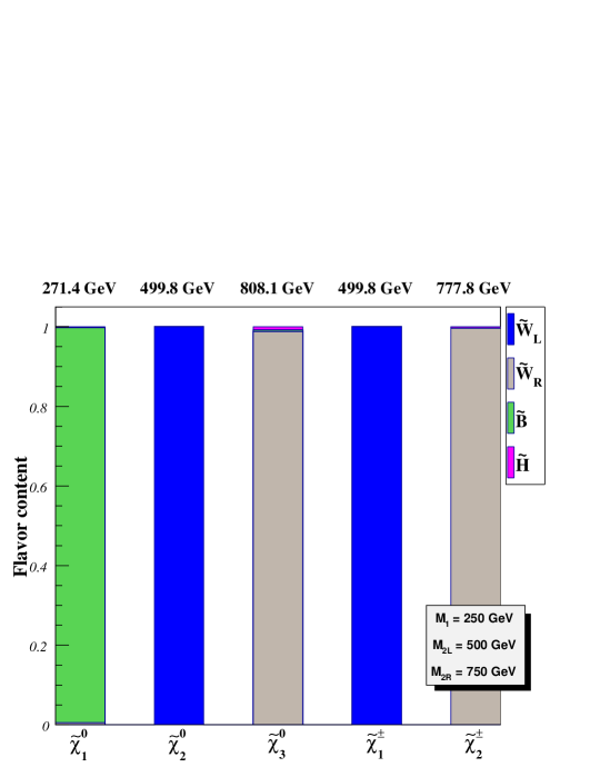
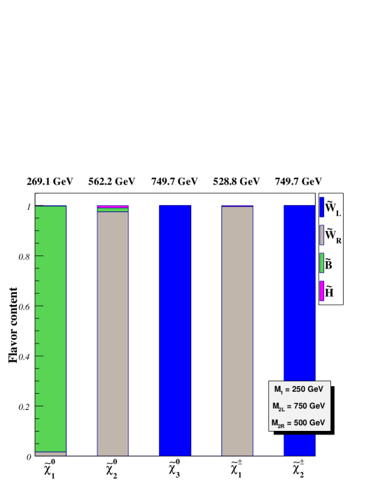
Figure 1: Flavor decomposition and masses of the lighter neutralino and chargino states for benchmark scenarios SI.1 (upper panel) and SI.2 (lower panel) as defined in Table 1. The bino, $SU(2)_{L}$ and $SU(2)_{R}$ wino components are presented in green, blue and gray, respectively, whilst the higgsino component is shown in pink.

Process	$~{}n=0~{}$	$~{}n=1~{}$	$~{}n=2~{}$
${\tilde{\chi}}_{2}^{0}\to{\tilde{\chi}}_{1}^{0}+n~{}\ell+X\quad$	0.57	0.08	0.35
${\tilde{\chi}}_{3}^{0}\to{\tilde{\chi}}_{1}^{0}+n~{}\ell+X\quad$	0.14	0.15	0.71
${\tilde{\chi}}_{1}^{\pm}\to{\tilde{\chi}}_{1}^{0}+n~{}\ell+X\quad$	0.22	0.78	0
${\tilde{\chi}}_{2}^{\pm}\to{\tilde{\chi}}_{1}^{0}+n~{}\ell+X\quad$	0.22	0.78	0

Process	$~{}n=0~{}$	$~{}n=1~{}$	$~{}n=2~{}$
${\tilde{\chi}}_{2}^{0}\to{\tilde{\chi}}_{1}^{0}+n~{}\ell+X\quad$	0.15	0.15	0.70
${\tilde{\chi}}_{3}^{0}\to{\tilde{\chi}}_{1}^{0}+n~{}\ell+X\quad$	0.57	0.08	0.35
${\tilde{\chi}}_{1}^{\pm}\to{\tilde{\chi}}_{1}^{0}+n~{}\ell+X\quad$	0.22	0.78	0
${\tilde{\chi}}_{2}^{\pm}\to{\tilde{\chi}}_{1}^{0}+n~{}\ell+X\quad$	0.22	0.78	0

Table 2: Branching ratios of the lighter neutralinos and charginos into charged leptons for scenario SI.1 (upper panel) and SI.2 (lower panel) after fixing the slepton and sneutrino masses to 400 GeV. The decays of the intermediate tau leptons, sleptons and sneutrinos are included. The symbol $X$ stands for missing energy or jets.

In these two non-mixing scenarios, winos decays are driven by the slepton masses $m_{\tilde{L}_{L}}$ and $m_{\tilde{L}_{R}}$. As neutral and charged winos originating from the same $SU(2)$ triplet are almost mass-degenerate, a specific (neutral or charged) wino can only decay into sleptons and sneutrinos of the corresponding chirality, together with the associated Standard Model partner. Sleptons and sneutrinos further decay into the bino state (the LSP), together with one additional lepton or neutrino, since their chirality prevents them from decaying into the other wino state, even if kinematically allowed. Depending on the difference between the wino and slepton masses, the decay process consists either of a cascade of two two-body decays, or of a prompt three-body decay mediated by a virtual slepton or sneutrino. This process leads to at most two charged leptons produced in association with missing energy related to the possible presence of final state neutrinos and the one of the stable and invisible bino. This kind of cascade decay is similar to those in the MSSM. The relevant branching ratios of the lighter neutralinos and charginos to leptons are indicated in Table 2, assuming a universal slepton mass of 400 GeV.

For our third benchmark scenario, we choose a typical mixing scenario. In this case, $SU(2)_{L}$ winos are mostly pure, whilst $SU(2)_{R}$ winos mix significantly with the bino field. This mimics the neutral and charged gauge boson mixing pattern presented in Appendix B, where $SU(2)_{R}\times U(1)_{B-L}$ is first broken to the hypercharge symmetry group, implying a mixing of the $W_{R}^{3}$ and $\hat{B}$ gauge boson. In a similar fashion, the $\tilde{W}_{R}^{3}$ and $\tilde{\hat{B}}$ mix, which yields the hypercharge bino $\tilde{B}^{\prime}$. In a second step, the electroweak gauge group is broken down to electromagnetism and the $\tilde{B}^{\prime}$ field mixes with the $\tilde{W}_{L}^{3}$ field. As in the MSSM, this mixing is in general rather small. This pattern is illustrated in scenario SII. The corresponding free parameters are presented in Table 1. The Higgs sector parameters are fixed slightly differently from scenarios SI.1 and SI.2 and we choose $M_{1}=100$ GeV, $M_{2L}=250$ GeV and $M_{2R}=150$ GeV, the lower bino mass ensuring a lightest supersymmetric particle which is neutral. Although the resulting mass of the lightest neutralino of 111 GeV and the one of the lightest chargino of about 200 GeV seem ruled out by current searches for electroweak superpartners at the LHC Aad:2012pxa ; Aad:2012hba ; ATLAS:2012kma ; Aad:2012jja ; Chatrchyan:2012pka ; Chatrchyan:2012mea ; Chatrchyan:2011ff ; CMS:aro , the present constraints are evaded in the case of scenario SII. First, model independent searches always assume a specific decay pattern (with a branching fraction of 100%) in the context of the MSSM. Next, already with a lightest neutralino mass of more than 110 GeV, the searches lose sensitivity to lighter charginos so that chargino masses of ${\cal O}(200~{}\text{GeV})$ are acceptable.

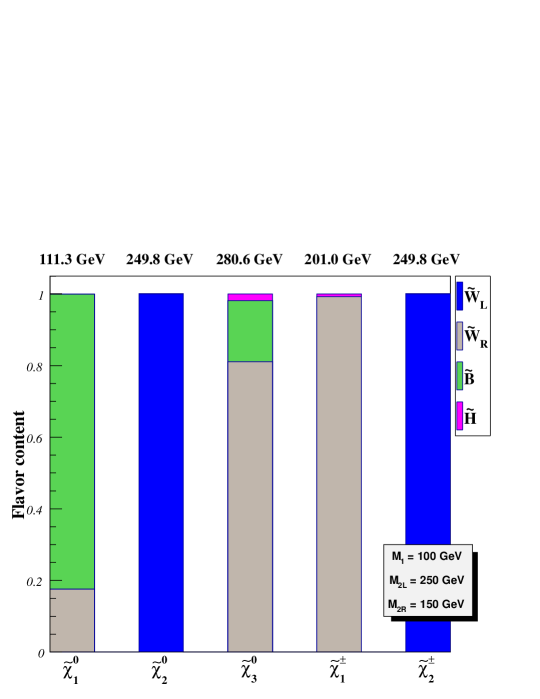
Figure 2: Same as in Figure 1 but for our benchmark scenario SII.

The flavor decomposition of the five lighter neutralino and chargino states is given in Figure 2, together with their mass eigenvalues. One observes a rather important bino-right wino mixing (of order $20\%$) among the first and third neutralino states. This opens new production channels for gaugino pairs, since, e.g., the first chargino can now be produced in association with both the first and the third neutralinos, and new decay channels are also possible. For instance, the third neutralino can decay to the lightest neutralino, in association with a $Z$-boson or a photon (the $Z^{\prime}$-boson being too heavy), this new decay process leading to a final state with at most two charged leptons and a significant amount of missing energy. Furthermore, if the charged sleptons are lighter than the third neutralino, the latter could also decay into a left-handed slepton-lepton pair. The produced slepton decays further, producing another lepton and missing energy. The decay patterns are illustrated in the upper and lower panels of Table 3, where we show them for different universal slepton masses, chosen equal to 200 GeV and 400 GeV, respectively. One observes than as soon as the charged current decay channel of the third neutralino into a chargino is open, it becomes significant and reduces the production of leptons from the SUSY particle decays.

Process	$~{}n=0~{}$	$~{}n=1~{}$	$~{}n=2~{}$
${\tilde{\chi}}_{2}^{0}\to{\tilde{\chi}}_{1}^{0}+n~{}\ell+X\quad$	0.57	0.08	0.35
${\tilde{\chi}}_{3}^{0}\to{\tilde{\chi}}_{1}^{0}+n~{}\ell+X\quad$	0.26	0.13	0.61
${\tilde{\chi}}_{1}^{\pm}\to{\tilde{\chi}}_{1}^{0}+n~{}\ell+X\quad$	1	0	0
${\tilde{\chi}}_{2}^{\pm}\to{\tilde{\chi}}_{1}^{0}+n~{}\ell+X\quad$	0.22	0.78	0

Process	$~{}n=0~{}$	$~{}n=1~{}$	$~{}n=2~{}$
${\tilde{\chi}}_{2}^{0}\to{\tilde{\chi}}_{1}^{0}+n~{}\ell+X\quad$	0.57	0.08	0.35
${\tilde{\chi}}_{3}^{0}\to{\tilde{\chi}}_{1}^{0}+n~{}\ell+X\quad$	0.12	0.09	0.43
${\tilde{\chi}}_{3}^{0}\to{\tilde{\chi}}_{1}^{\pm}+n~{}\ell+X\quad$	0.35	0	0
${\tilde{\chi}}_{1}^{\pm}\to{\tilde{\chi}}_{1}^{0}+n~{}\ell+X\quad$	1	0	0
${\tilde{\chi}}_{2}^{\pm}\to{\tilde{\chi}}_{1}^{0}+n~{}\ell+X\quad$	0.22	0.78	0

Table 3: Branching ratios of the lighter neutralinos and charginos into charged leptons for the scenario SII with a universal slepton soft mass of 200 (upper panel) and 400 (lower panel) GeV. The decays of the intermediate tau lepton, sleptons and sneutrinos are included. The symbol $X$ stands for missing energy or jets.

More interestingly, some specific hierarchies of the three soft gaugino masses yield a large mixing in the neutralino sector. We design our fourth and last benchmark point as a representative of these scenarios. With the choice of parameters presented in the last column of Table 1, one obtains the flavor decomposition of the five lighter neutralinos and charginos presented in Figure 3. In this case, the three soft gaugino masses are rather close to each other, i.e., $M_{1}=359$ GeV, $M_{2L}=320$ GeV and $M_{2R}=270$ GeV, which leads to a significant mixing pattern. Moreover, two charginos and two neutralinos are very close in mass, which could lead to displaced vertices, the next-to-lightest neutralino and the two lighter charginos having a lifetime of 4.13 ns, 0.09 ns and 1.09 ns, up to a possible boost factor, respectively. This corresponds to decay lengths ranging from the order of the centimeter to the meter. Furthermore, as in scenario SII, such a gaugino hierarchy leads to possibly lepton-enriched decay chains, although the produced leptons are expected to be very soft due to the compression of the mass spectrum. The branching ratios of the lighter neutralinos and charginos, for typical slepton masses of 400 GeV, are shown in Table 4. Sleptons and sneutrinos have hence been chosen heavier than most of the lighter neutralino and chargino states. However, when real and not virtual, they decay further mainly to the lightest chargino (64%) and to the second lightest neutralino (36%) whilst sneutrinos decay to the lightest chargino (64%) and to the lightest (21%) and the next-to-lightest (15%) neutralinos.

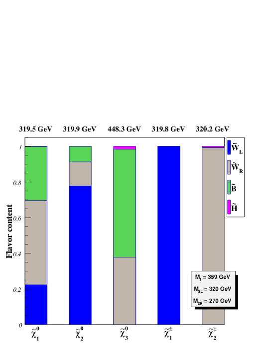
Figure 3: Same as in Figure 1 but for our benchmark scenario SIII.

Process	$~{}n=0~{}$	$~{}n=1~{}$	$~{}n=2~{}$
${\tilde{\chi}}_{2}^{0}\to{\tilde{\chi}}_{1}^{0}+n~{}\ell+X\quad$	0.22	0	0.16
${\tilde{\chi}}_{2}^{0}\to{\tilde{\chi}}_{1}^{\pm}+n~{}\ell+X\quad$	0.52	0.10	0
${\tilde{\chi}}_{3}^{0}\to{\tilde{\chi}}_{1}^{0}+n~{}\ell+X\quad$	0.10	0	0
${\tilde{\chi}}_{3}^{0}\to{\tilde{\chi}}_{2}^{0}+n~{}\ell+X\quad$	0.10	0.03	0.13
${\tilde{\chi}}_{3}^{0}\to{\tilde{\chi}}_{1}^{\pm}+n~{}\ell+X\quad$	0.14	0.51	0
${\tilde{\chi}}_{1}^{\pm}\to{\tilde{\chi}}_{1}^{0}+n~{}\ell+X\quad$	0.84	0.16	0
${\tilde{\chi}}_{2}^{\pm}\to{\tilde{\chi}}_{1}^{0}+n~{}\ell+X\quad$	0.996	0	0
${\tilde{\chi}}_{2}^{\pm}\to{\tilde{\chi}}_{2}^{0}+n~{}\ell+X\quad$	0.004	0	0

Table 4: Branching ratios of the lighter neutralinos and charginos into charged leptons for the scenario SIII with a universal slepton soft mass of 400 GeV. The decays of the intermediate tau leptons, sleptons and sneutrinos are included. The symbol $X$ stands for missing energy or jets.

4 Gauginos as probes of left-right symmetric supersymmetry at the LHC

4.1 General considerations

Process	$\sqrt{S}=7$ TeV [fb]	$\sqrt{S}=8$ TeV [fb]	$\sqrt{S}=14$ TeV [fb]
$pp\to{\tilde{\chi}}_{2}^{0}{\tilde{\chi}}_{1}^{\pm}\quad$	$\quad 13.2\quad$	$\quad 20.6\quad$	$\quad 89.6\quad$
$pp\to{\tilde{\chi}}_{3}^{0}{\tilde{\chi}}_{2}^{\pm}\quad$	$\quad 0.71\quad$	$\quad 1.40\quad$	$\quad 11.4\quad$
$pp\to{\tilde{\chi}}_{1}^{0}{\tilde{\chi}}_{2}^{\pm}\quad$	$\quad<0.1\quad$	$\quad<0.1\quad$	$\quad 0.39\quad$
$pp\to{\tilde{\chi}}_{1}^{+}{\tilde{\chi}}_{1}^{-}\quad$	$\quad 2.90\quad$	$\quad 4.61\quad$	$\quad 21.2\quad$
$pp\to{\tilde{\chi}}_{2}^{+}{\tilde{\chi}}_{2}^{-}\quad$	$\quad 0.21\quad$	$\quad 0.42\quad$	$\quad 3.41\quad$

Process	$\sqrt{S}=7$ TeV [fb]	$\sqrt{S}=8$ TeV [fb]	$\sqrt{S}=14$ TeV [fb]
$pp\to{\tilde{\chi}}_{2}^{0}{\tilde{\chi}}_{1}^{\pm}\quad$	$\quad 10.2\quad$	$\quad 16.3\quad$	$\quad 76.0\quad$
$pp\to{\tilde{\chi}}_{3}^{0}{\tilde{\chi}}_{2}^{\pm}\quad$	$\quad 0.98\quad$	$\quad 1.86\quad$	$\quad 13.8\quad$
$pp\to{\tilde{\chi}}_{1}^{0}{\tilde{\chi}}_{1}^{\pm}\quad$	$\quad 1.16\quad$	$\quad 1.67\quad$	$\quad 5.88\quad$
$pp\to{\tilde{\chi}}_{1}^{+}{\tilde{\chi}}_{1}^{-}\quad$	$\quad 4.49\quad$	$\quad 7.13\quad$	$\quad 32.9\quad$
$pp\to{\tilde{\chi}}_{2}^{+}{\tilde{\chi}}_{2}^{-}\quad$	$\quad 0.21\quad$	$\quad 0.40\quad$	$\quad 3.14\quad$

Table 5: Dominant cross sections, given in fb and at the leading order of perturbative QCD, of neutralino and chargino pair production at the LHC for a center-of-mass energy of 7 TeV, 8 TeV and 14 TeV. Results are shown for benchmark scenarios SI.1 (upper panel) and SI.2 (lower panel) after setting the slepton masses to a universal value of 400 GeV.

Process	$\sqrt{S}=7$ TeV [fb]	$\sqrt{S}=8$ TeV [fb]	$\sqrt{S}=14$ TeV [fb]
$pp\to{\tilde{\chi}}_{3}^{0}{\tilde{\chi}}_{1}^{\pm}\quad$	$\quad 4999\quad$	$\quad 6530\quad$	$\quad 17490\quad$
$pp\to{\tilde{\chi}}_{1}^{0}{\tilde{\chi}}_{1}^{\pm}\quad$	$\quad 3139\quad$	$\quad 4085\quad$	$\quad 10830\quad$
$pp\to{\tilde{\chi}}_{2}^{0}{\tilde{\chi}}_{2}^{\pm}\quad$	$\quad 387\quad$	$\quad 514\quad$	$\quad 1452\quad$
$pp\to{\tilde{\chi}}_{2}^{0}{\tilde{\chi}}_{1}^{\pm}\quad$	$\quad 0.83\quad$	$\quad 1.09\quad$	$\quad 2.88\quad$
$pp\to{\tilde{\chi}}_{3}^{0}{\tilde{\chi}}_{2}^{\pm}\quad$	$\quad<0.1\quad$	$\quad<0.1\quad$	$\quad 0.11\quad$
$pp\to{\tilde{\chi}}_{1}^{+}{\tilde{\chi}}_{1}^{-}\quad$	$\quad 532\quad$	$\quad 780\quad$	$\quad 2851\quad$
$pp\to{\tilde{\chi}}_{2}^{+}{\tilde{\chi}}_{2}^{-}\quad$	$\quad 92.2\quad$	$\quad 123\quad$	$\quad 355.9\quad$

Process	$\sqrt{S}=7$ TeV [fb]	$\sqrt{S}=8$ TeV [fb]	$\sqrt{S}=14$ TeV [fb]
$pp\to{\tilde{\chi}}_{3}^{0}{\tilde{\chi}}_{1}^{\pm}\quad$	$\quad 5188\quad$	$\quad 6776\quad$	$\quad 18140\quad$
$pp\to{\tilde{\chi}}_{1}^{0}{\tilde{\chi}}_{1}^{\pm}\quad$	$\quad 3255\quad$	$\quad 4236\quad$	$\quad 11230\quad$
$pp\to{\tilde{\chi}}_{2}^{0}{\tilde{\chi}}_{2}^{\pm}\quad$	$\quad 387\quad$	$\quad 514\quad$	$\quad 1451\quad$
$pp\to{\tilde{\chi}}_{2}^{0}{\tilde{\chi}}_{1}^{\pm}\quad$	$\quad 0.86\quad$	$\quad 1.13\quad$	$\quad 3\quad$
$pp\to{\tilde{\chi}}_{3}^{0}{\tilde{\chi}}_{2}^{\pm}\quad$	$\quad<0.1\quad$	$\quad<0.1\quad$	$\quad 0.11\quad$
$pp\to{\tilde{\chi}}_{1}^{+}{\tilde{\chi}}_{1}^{-}\quad$	$\quad 572\quad$	$\quad 838\quad$	$\quad 3059\quad$
$pp\to{\tilde{\chi}}_{2}^{+}{\tilde{\chi}}_{2}^{-}\quad$	$\quad 92.2\quad$	$\quad 123\quad$	$\quad 356\quad$

Process	$\sqrt{S}=7$ TeV [fb]	$\sqrt{S}=8$ TeV [fb]	$\sqrt{S}=14$ TeV [fb]
$pp\to{\tilde{\chi}}_{2}^{0}{\tilde{\chi}}_{1}^{\pm}\quad$	$\quad 99.6\quad$	$\quad 137\quad$	$\quad 433\quad$
$pp\to{\tilde{\chi}}_{1}^{0}{\tilde{\chi}}_{2}^{\pm}\quad$	$\quad 93.6\quad$	$\quad 128\quad$	$\quad 393\quad$
$pp\to{\tilde{\chi}}_{1}^{0}{\tilde{\chi}}_{1}^{\pm}\quad$	$\quad 28.5\quad$	$\quad 39.3\quad$	$\quad 125\quad$
$pp\to{\tilde{\chi}}_{2}^{0}{\tilde{\chi}}_{2}^{\pm}\quad$	$\quad 26.7\quad$	$\quad 36.6\quad$	$\quad 113\quad$
$pp\to{\tilde{\chi}}_{3}^{0}{\tilde{\chi}}_{2}^{\pm}\quad$	$\quad 13.0\quad$	$\quad 19.0\quad$	$\quad 69.2\quad$
$pp\to{\tilde{\chi}}_{2}^{+}{\tilde{\chi}}_{2}^{-}\quad$	$\quad 537\quad$	$\quad 788\quad$	$\quad 2887\quad$
$pp\to{\tilde{\chi}}_{1}^{+}{\tilde{\chi}}_{1}^{-}\quad$	$\quad 29.8\quad$	$\quad 41.7\quad$	$\quad 137\quad$

Table 6: Same as in Table 5, but for benchmark scenarios SII after setting the slepton masses to a universal value of 200 GeV (upper panel) and 400 GeV (middle panel) and for scenario SIII with a universal slepton mass of 400 GeV (lower panel).

At the LHC, neutralinos $\tilde{\chi}^{0}$ and charginos $\tilde{\chi}^{\pm}$ can be produced directly in pairs or in association with gluinos $\tilde{g}$ or with squarks $\tilde{q}$. In the scenarios considered in this work, squarks and gluinos are very heavy and decoupled. Therefore, the only relevant production processes are

$$p\ p\rightarrow\tilde{\chi}_{i}^{\mp}\tilde{\chi}_{j}^{\pm}\ ,\quad\tilde{\chi}_{i}^{0}\tilde{\chi}_{j}^{0}\quad\text{and}\quad\tilde{\chi}_{i}^{0}\tilde{\chi}_{j}^{\pm}\ ,$$ (42)

via $s$-channel gauge boson exchange or $t/u$-channel squark exchange. Although existing bounds on the $Z_{R}$ and $W_{R}$ boson masses Beringer:2012zz force them to be heavy, pair production of the neutralino and chargino states through one of the new vector boson is not necessarily suppressed at the LHC energies, as the cross section may get enhanced by important (although not considered in this work) resonance effects. In addition, the decoupling of squarks also leads to an increase in the cross section, taming the destructive interferences between the $s$- and $t/u$-channel diagrams. In Table 5 and Table 6 we present numerical predictions for the most relevant associated production cross sections at the LHC, running at a center-of-mass energy of 7 TeV (2010-2011 run), 8 TeV (2012 run) and 14 TeV (future run). Numerical computations have been performed using the matrix element generator MadGraph 5 Alwall:2011uj , after convoluting the produced hard-scattering squared matrix elements with the leading order set of parton densities CTEQ6L1 Pumplin:2002vw . The LRSUSY UFO files Degrande:2011ua necessary for MadGraph 5 have been generated with the program FeynRules Christensen:2008py ; Christensen:2009jx ; Christensen:2010wz ; Duhr:2011se ; Fuks:2012im ; Alloul:2013fw after implementing the Lagrangian introduced in Section 2. The results shown in the tables correspond to a factorization scale fixed to the transverse mass of the produced superparticles and are given at the leading-order of perturbative QCD. We omit all channels involving a cross section smaller than 0.1 fb and set the slepton and sneutrino masses to 400 GeV, unless otherwise stated.

Considering neutralino and chargino production in the MSSM, more precise calculations are available once we add next-to-leading order corrections Beenakker:1999xh ; Debove:2010kf combined with the resummation of the leading and next-to-leading logarithms to all orders in the strong coupling Debove:2009ia ; Debove:2010kf ; Debove:2011xj . This is known to increase the cross sections by about $20\%-25\%$. Although no such precision computations have been achieved in the LRSUSY context, the structure of the next-to-leading order calculations is very similar in both the MSSM and the LRSUSY cases. We therefore adopt, in the rest of this paper, next-to-leading values to be equal to leading-order results for LRSUSY signal cross sections multiplied by constant $K$-factor fixed to $1.20$.

Once produced, all neutralinos and charginos decay into isolated leptons, hard jets and missing energy carried by the LSPs by means of cascades of two-body (and possibly three-body) decays. We choose to focus on the pattern with the cleanest collider signature, when several hard isolated leptons are produced. For instance, a typical gaugino cascade decay would be

$$\begin{split}\mbox{(heavy chargino/neutralino)}&\rightarrow\mbox{(lepton)}\;\mbox{(slepton)}^{(\star)}\\ &\rightarrow\mbox{(lepton)}\;\mbox{(lepton)}\;\mbox{(light chargino/neutralino)}\ ,\end{split}$$ (43)

where the (slepton)^(⋆) is a real (virtual) slepton, as lighter (heavier) than the heavy chargino or neutralino. Channels with intermediate gauge bosons are sometimes open and lead to similar final state signatures. Although such cascades exist in both MSSM and LRSUSY models, an explicit analysis of the neutralino and chargino production and decays could be useful to unveil differences between the two symmetries. In principle, while the final state signatures are very similar in terms of number of leptons, jets and missing energy, the intermediate decay stages could be different, yielding different results in terms of branching ratios and kinematical distributions.

Process	Signature	Representative candidate processes
I.	$0\,\ell+\not{E}_{T}$	$p\,p\rightarrow\tilde{\chi}_{1}^{0}\tilde{\chi}_{1}^{0}$
II.	$1\,\ell+\not{E}_{T}$	$p\,p\rightarrow\left(\tilde{\chi}_{1}^{\pm}\rightarrow\ell^{\pm}{\nu}_{\ell}\tilde{\chi}_{1}^{0}\right)\,\tilde{\chi}_{1}^{0}$
III.A	$2\,\ell+\not{E}_{T}$	$p\,p\rightarrow\left(\tilde{\chi}_{2}^{0}\rightarrow\ell^{\pm}{\ell}^{\mp}\tilde{\chi}_{1}^{0}\right)\,\tilde{\chi}_{1}^{0}$
III.B		$p\,p\rightarrow\left(\tilde{\chi}_{1}^{\pm}\rightarrow\ell^{\pm}{\nu}_{\ell}\tilde{\chi}_{1}^{0}\right)\,\left(\tilde{\chi}_{1}^{\mp}\rightarrow\ell^{\prime\mp}{\nu}_{\ell^{\prime}}\tilde{\chi}_{1}^{0}\right)$
IV.	$3\,\ell+\not{E}_{T}$	$p\,p\rightarrow\left(\tilde{\chi}_{2}^{0}\rightarrow\ell^{\pm}{\ell}^{\mp}\tilde{\chi}_{1}^{0}\right)\,\left(\tilde{\chi}_{1}^{\pm}\rightarrow\ell^{\prime\pm}{\nu}_{\ell^{\prime}}\tilde{\chi}_{1}^{0}\right)$
V.A	$4\,\ell+\not{E}_{T}$	$p\,p\rightarrow\left(\tilde{\chi}_{2}^{0}\rightarrow\ell^{\pm}{\ell}^{\mp}\tilde{\chi}_{1}^{0}\right)\,\left(\tilde{\chi}_{2}^{0}\rightarrow\ell^{\prime\pm}{\ell}^{\prime\mp}\tilde{\chi}_{1}^{0}\right)\,$
V.B		$p\,p\rightarrow\left(\tilde{\chi}_{1}^{\mp}\rightarrow\ell^{\mp}{\nu}_{\ell}\tilde{\chi}_{1}^{0}\right)\,\left(\tilde{\chi}_{3}^{0}\rightarrow\ell^{\prime\pm}\ell^{\prime\prime\pm}{\ell}^{\prime\prime\mp}{\nu}_{\ell^{\prime}}jj\tilde{\chi}_{1}^{0}\right)$
VI.	$5\,\ell+\not{E}_{T}$	$p\,p\rightarrow\left(\tilde{\chi}_{3}^{0}\rightarrow\ell^{\pm}{\ell}^{\mp}\ell^{\prime\pm}{\ell}^{\prime\mp}\tilde{\chi}_{1}^{0}\right)\,\left(\tilde{\chi}_{1}^{\pm}\rightarrow\ell^{\prime\prime\pm}\nu_{\ell^{\prime\prime}}\tilde{\chi}_{1}^{0}\right)$
VII.	$6\,\ell+\not{E}_{T}$	$p\,p\rightarrow\left(\tilde{\chi}_{3}^{0}\rightarrow\ell^{\pm}{\ell}^{\mp}\ell^{\prime\pm}{\ell}^{\prime\mp}\tilde{\chi}_{1}^{0}\right)\,\left(\tilde{\chi}_{2}^{0}\rightarrow\ell^{\prime\prime\pm}{\ell}^{\prime\prime\mp}\tilde{\chi}_{1}^{0}\right)\,$
VIII.	$7\,\ell+\not{E}_{T}$	$p\,p\rightarrow\left(\tilde{\chi}_{3}^{0}\rightarrow\ell^{\pm}{\ell}^{\mp}\ell^{\prime\pm}{\ell}^{\prime\mp}\tilde{\chi}_{1}^{0}\right)\,\left(\tilde{\chi}_{3}^{0}\rightarrow\ell^{\prime\prime\pm}\ell^{\prime\prime\prime\pm}{\ell}^{\prime\prime\prime\mp}{\nu}_{\ell^{\prime\prime}}jj\tilde{\chi}_{1}^{0}\right)$
IX.	$8\,\ell+\not{E}_{T}$	$p\,p\rightarrow\left(\tilde{\chi}_{3}^{0}\rightarrow\ell^{\pm}{\ell}^{\mp}\ell^{\prime\pm}{\ell}^{\prime\mp}\tilde{\chi}_{1}^{0}\right)\,\left(\tilde{\chi}_{3}^{0}\rightarrow\ell^{\prime\prime\pm}{\ell}^{\prime\prime\mp}\ell^{\prime\prime\prime\pm}{\ell}^{\prime\prime\prime\mp}\tilde{\chi}_{1}^{0}\right)$

Table 7: Multilepton LHC signatures related to chargino and neutralino production and decays in LRSUSY models. As each type of signature receives contributions from one or more decay processes, we only give a few representative examples.

In the MSSM, gaugino cascade decays as above involve both hypercharge and/or $SU(2)_{L}$ gauginos. In LRSUSY models, the field content is supplemented by new neutral and charged gauge fermions, and the hypercharge bino state originates from the mixing of the $B-L$ bino and $SU(2)_{R}$ neutral wino. Gaugino decay chains could hence acquire novel features not present in the MSSM. For example, we start from the MSSM decay

$$\tilde{W}_{L}^{3}\rightarrow\ell_{L}^{+}\tilde{\ell}_{L}^{\star-}\rightarrow\ell^{+}\ell^{-}\tilde{B}^{\prime}\ .$$ (44)

As the $\tilde{W}_{L}^{3}$ and $\tilde{W}_{L}^{\pm}$ fields are nearly mass-degenerate since $SU(2)_{L}$ breaking splitting effects are small, gaugino-to-gaugino decays are hardly possible. The winos then mostly decay through (virtual or real) sleptons, which yields signatures with at most two charged leptons. In contrast, LRSUSY gaugino-to-gaugino decays are possible, as for example in the case of the benchmark scenarios SII and SIII (see Table 3 and Table 4), where the physical states are admixtures of different gaugino states (see Figure 2 and Figure 3). This leads to lepton-enriched decay chains such as

$$\tilde{W}^{0}_{R}\rightarrow\ell_{R}^{+}\tilde{\ell}_{R}^{(\star)-}\rightarrow\ell_{R}^{+}\ell_{R}^{-}\tilde{\chi}_{2}^{0}\rightarrow\ell_{R}^{+}\ell_{R}^{-}{\ell}_{L}^{\prime\,+}\tilde{\ell}_{L}^{(\star)\prime\,-}\rightarrow\ell_{R}^{+}\ell_{R}^{-}{\ell}_{L}^{\prime\,+}{\ell}_{L}^{\prime\,-}\tilde{\chi}^{0}_{1}\ ,$$ (45)

where the two lighter neutralinos have both $B-L$ bino and $SU(2)_{L}$ wino components. In this case, the decay yields a tetralepton plus missing energy final state. Whereas allowing for immediately distinguishing LRSUSY models from the MSSM, these types of signatures suffer from very low branching fractions in our scenarios and, depending on final state lepton hardness, could be difficult to observe.

We generically classify the different final state signatures possibly arising from the production and decay of two gauginos in LRSUSY models in Table 7. Our classification is based on the number of produced leptons determined by the production and decay of the five LRSUSY gaugino states. For each type of signature, we give one representative associated process. In contrast to the MSSM where the number of produced leptons is limited to at most four (considering only the lightest chargino and the two lighter neutralinos), LRSUSY models feature the production of final states with up to eight charged leptons, a Standard Model background free signature if the associated production rate is large enough.

In the rest of this section, we first (Section 4.2) focus on the possible extraction of a LRSUSY signal from the SM background in the context of the benchmark scenarios of Section 3. Next, in the eventuality of the observation of an excess of leptonic events at the LHC, we show, for similar mass spectra in the MSSM and LRSUSY cases, several ways to disentangle both models (Section 4.3).

4.2 Leptonic signatures of left-right symmetric gauginos at the LHC

We now concentrate on phenomenological analyses relying on Monte Carlo simulations of collisions produced at the LHC, for a center-of-mass energy of 8 TeV and an integrated luminosity of 20 fb^-1. For both signal and background, we make use of the MadGraph 5 Alwall:2011uj package for generating hard process matrix elements, including up to two additional jets for Standard Model contributions, convoluted with the parton density set CTEQ6L1 Pumplin:2002vw . Parton-level events were then matched to parton showering and hadronization by means of the program Pythia Sjostrand:2006za ; Sjostrand:2007gs and merged according to the $k_{T}$-MLM scheme Mangano:2006rw ; Alwall:2008qv . Focusing on leptonic final states, we assumed perfect electron and muon reconstruction. This is a fair approximation when one accounts for appropriate object selection criteria based on, e.g., large transverse momentum. Simulated events were eventually analyzed within the MadAnalysis 5 framework Conte:2012fm .

We generated dedicated event samples for various sources of Standard Model background and reweighted the samples according to calculations for the total production rates convoluting next-to-leading order (NLO) or even next-to-next-to-leading order (NNLO) matrix elements, when available, with the CT10 parton densities Lai:2010vv . Events originating from the leptonic or invisible decay of a $W$-boson or $Z$-boson produced in association with jets have been reweighted to the NNLO accuracy, using total rates of 35678 pb and 10319 pb, respectively, as predicted by the Fewz program Gavin:2012sy ; Gavin:2010az . Inclusive top-antitop events have been normalized to a cross section of 255.8 pb, as derived by the Hathor package Aliev:2010zk , which includes all NLO diagrams and genuine NNLO contributions, while single top event generation in the $t$-, $tW$- and $s$-channel topology has been normalized, at an approximate NNLO accuracy, to 87.2 pb, 22.2 pb and 5.5 pb, respectively Kidonakis:2012db . Diboson events have been rescaled to a weight derived from NLO results as computed by means of the Mcfm software, using cross sections of 30.2 pb, 11.8 pb and 4.5 pb for the $WW$, $WZ$ and $ZZ$ channels, respectively Campbell:1999ah ; Campbell:2011bn ; Campbell:2012dh . In this case, fully hadronic decay modes have been neglected. Next, $ttW$ and $ttZ$ events were normalized to NLO, using again Mcfm, while the normalization of the other simulated rare Standard Model processes relied on MadGraph 5 results. We hence employed cross sections of 0.25 pb, 0.21 pb, 46 fb, 13 fb and 0.7 fb, for the $ttW$, $ttZ$, $tZj$, $ttWW$ and $tttt$ channels, respectively. Finally, we did not consider multijet events, their correct treatment requiring data-driven methods. However, basing the analyses of this work on final states containing charged leptons with very large transverse momentum and a sensible quantity of missing transverse energy, we expect those contributions to be fully under control Aad:2012wm ; Chatrchyan:2012oaa .

We designed three analyses possibly sensitive to LRSUSY signals based on different event lepton multiplicity and subsequently divided the background and event samples in three categories. We separately considered events with one single lepton (see Section 4.2.1), two leptons (see Section 4.2.2) and more than two leptons (see Section 4.2.3). This distinction was made after defining jet and lepton candidates as follows.

• Jets are reconstructed by means of the FastJet program Cacciari:2005hq ; Cacciari:2011ma , using an anti-$k_{t}$ algorithm of radius parameter $R=0.4$ Cacciari:2008gp .

• We only retain jet candidates if their transverse momentum is greater than 20 GeV and their pseudorapidity fulfills $|\eta|\leq 2.5$.

• We select electrons and muons candidates having a transverse momentum $p_{T}$ larger than 10 GeV and a pseudorapidity $|\eta|\leq 2.5$.

• We remove jet objects which lie in an angular distance $\Delta R=\sqrt{\Delta\phi^{2}+\Delta\eta^{2}}\leq 0.1$ of an electron, where $\phi$ stands for the azimuthal angle with respect to the beam direction.

• We remove electrons and muons lying in a cone of radius $\Delta R\leq 0.4$ of any of the remaining jets.

We then vetoed events containing at least one $b$-tagged jet, including a $b$-tagging efficiency of 60% for a charm/light mistagging rate of 10%/1%.

4.2.1 A single lepton signature

As deduced from the branching ratio tables computed in Section 3, LRSUSY gaugino pair production at the LHC are likely to give rise to events containing exactly one charged lepton and a sensible amount of missing transverse energy carried by the undetected LSPs. The associated production cross section is however rather reduced in many cases, as shown in Table 5 and Table 6 for the benchmark scenarios under consideration, which may render the observation of any LRSUSY hint challenging. In this analysis, we select events with exactly $N_{\ell}=1$ charged lepton. After applying the object definitions above-mentioned, the signal efficiency ranges from less than 1% in the case of the SIII scenario, where most of the leptons are too soft to be detected due to small splittings in the mass spectrum (see Figure 3), to 42% for the scenario SI.1. At this stage, the SM background overwhelms the signal by more than four orders of magnitude and is dominated by $W$+jets events (94%) and $Z$+jets events (5.7%), where one of the lepton either lies outside the $\eta\leq 2.5$ region, or is too soft for being observed (with $p_{T}<10$ GeV), or is non-isolated. We recall that those numbers do not include non-simulated multijet background events possibly yielding final state signatures with charged leptons originating from the hadronization process.

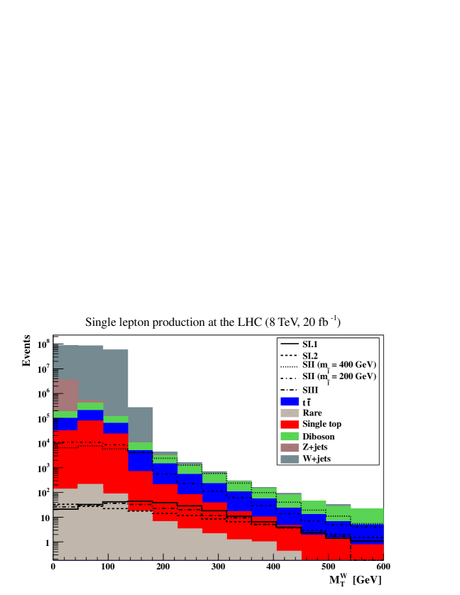
Figure 4: Distribution of the $M_{T}^{W}$ variable defined in Eq. (46) after selecting events with exactly one charged lepton and vetoing events with at least one $b$-tagged jet. We considered 20 fb^-1 of LHC collisions at a center-of-mass energy of 8 TeV and present results for the different background contributions and for all the considered LRSUSY scenarios.

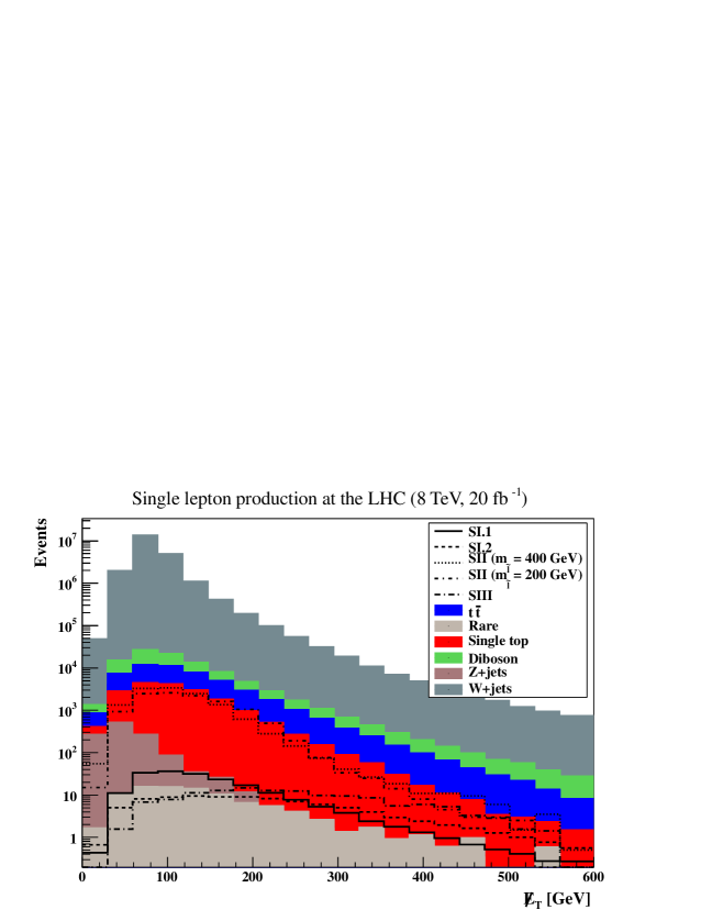
Figure 5: Missing transverse energy distribution after vetoing events with at least one $b$-tagged jet and selecting events with exactly one charged lepton and $M_{T}^{W}\geq 100$ GeV. We considered 20 fb^-1 of LHC collisions at a center-of-mass energy of 8 TeV and present results for the different background contributions and for all the considered LRSUSY scenarios.

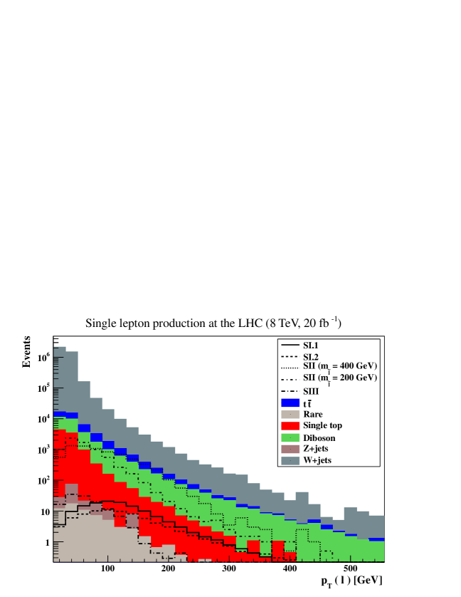
Figure 6: Transverse-momentum spectrum of the identified lepton, after vetoing events with at least one $b$-tagged jet and selecting events with exactly one charged lepton, $M_{T}^{W}\geq 100$ GeV and $\not{E}_{T}\geq 100$ GeV. We considered 20 fb^-1 of LHC collisions at a center-of-mass energy of 8 TeV and present results for the different background contributions and for all the considered LRSUSY scenarios.

In order to reduce the SM contamination, we impose a constraint on the kinematical variable

$$M_{T}^{W}=\sqrt{2p_{T}^{\ell}\not{E}_{T}\Big{[}1-\cos\Delta\phi_{\ell,\not{E}_{T}}\Big{]}}\ ,$$ (46)

where $\Delta\phi_{\ell,\not{E}_{T}}$ stands for the angular distance, in the azimuthal direction with respect to the beam, between the lepton and the missing energy. This variable would be the $W$-boson transverse mass in the case where all the missing energy and the identified lepton both originate from a $W$-boson decay. This quantity is expected to be smaller in the context of the Standard Model, as illustrated on Figure 4, than in the LRSUSY case, which features cascade decays to multiple final state particles contributing to the missing energy. In Figure 4, we show results for the different contributions to the SM background, upon which we superimpose signal distributions for the LRSUSY scenarios designed in Section 3. For the sake of simplicity, we fix the universal slepton masses to 400 GeV in all cases but for the scenario SII, where we consider both light and heavy sleptons with a mass fixed either to 200 GeV or to 400 GeV.

On the basis of these results, we require the $W$-boson transverse mass to satisfy $M_{T}^{W}~{}\geq~{}100$ GeV. This reduces the background by a factor of 10, which is however still dominated by $W$+jets events (99.6%). Subdominant contributions include diboson events and $t\bar{t}$ events associated with topologies where possibly one or several leptons are not reconstructed. In contrast, $30\%-45\%$ (scenario SII), $60\%-75\%$ (scenarios SI.1 and SI.2) and $70\%$ (scenario SIII) of the signal events so far selected survive.

In Figure 5, we present the other key observable of this single lepton analysis, the missing transverse energy spectrum. One observes that the dominant background contributions can be further suppressed by requiring large missing energy $\not{E}_{T}\geq 100$ GeV. Once again, this selection does not affect the signal too much, 55% to 99% of the events surviving in all scenarios, whereas the number of remaining background events is reduced by a factor of six. The background consists still in 95.4% of the cases of $W$+jets events. As shown in many experimental analyses, a combined selection on the missing energy and on the $W$-boson transverse mass also allows to keep the (non-simulated) multijet background under control (see, e.g., Ref. Aad:2012wm ), which justifies not considering them.

In Figure 6, we depict the lepton transverse-momentum distribution for the background and the different signal scenarios. When large mass splittings are present in LRSUSY spectra, gaugino-to-gaugino cascades induce very hard leptons as, e.g., in scenarios SI.1, SI.2 and SII, in particular when sleptons are heavy. In this case, the tails of the $p_{T}$ distributions even extend to values greater than 200 GeV. These first two benchmarks however suffer from very small signal cross sections, whereas the scenario SII could lead to a promising discovery channel for LRSUSY as gaugino mixing allows to produce new physics events at a larger rate. In contrast, for compressed LRSUSY spectra such as in scenario SIII, we expect much softer leptons. The lepton transverse momentum distribution indeed has its maximum at a $p_{T}$ value very close to the background one. We optimized our selection focusing on the most promising cases and imposed $p_{T}(\ell)\geq 80$ GeV. This leads to a good background rejection of a factor of about 3 together with a large signal efficiency of 50%-70% in the relevant cases (and a smaller one for scenarios unlikely to be observed).

Scenario	Signal ($S$)	Background ($B$)	$S/\sqrt{S+B}$
SI.1	$94.9\pm 8.2$	$55332\pm 247$	$0.40\pm 0.08$
SI.2	$56.1\pm 7.8$		$0.24\pm 0.07$
SII (200 GeV sleptons)	$1594\pm 44$		$6.68\pm 0.36$
SII (400 GeV sleptons)	$3334\pm 63$		$13.8\pm 0.5$
SIII	$31.8\pm 6.2$		$0.13\pm 0.05$

Table 8: Number of expected single-lepton events for 20 fb^-1 of LHC collisions at a center-of-mass energy of 8 TeV, given together with the associated statistical uncertainties, after applying all the selections described in the text. We present numbers of event $S$ for each of the signal scenarios introduced in Section 3 after including a NLO $K$-factor set to 1.2 and for the background ($B$). The results are then converted in terms of LHC significance to LRSUSY signals in singly-leptonic final states.

After all selections, one finds that a very simple analysis based on a single lepton plus missing energy topology is not suitable to probe most of the typical LRSUSY scenarios with light gauginos and heavy higgsinos that can be built from low energy considerations. An exception is benchmark point SII featuring sensible gaugino mixings and enough mass splitting between the mass eigenstates such that hard enough leptons are produced in their decays. In this case, a sensitivity, defined as the ratio of the number of selected signal events ($S$) to the squared root of all selected signal ($S$) and background ($B$) events ($\sqrt{S+B}$), of more than $5\sigma$ is expected for both SII scenarios with 200 GeV and 400 GeV slepton masses. In Table 8 we summarize the results, expressed in terms of number of events surviving all selections and LHC sensitivity, for each of the considered signal scenarios.

4.2.2 A dileptonic signature

Based on the branching ratio tables of Section 3, dileptonic signatures are foreseen to be quite frequent in the decay of a gaugino pair. They arise either from the dileptonic decay of the first gaugino and a full hadronic or invisible decay of the second one, or from the singly-leptonic decay of both superpartners. When accounting for geometrical acceptance ($|\eta(\ell)|\leq 2.5$), transverse-momentum threshold ($p_{T}(\ell)\geq 10$ GeV) and isolation criteria (removal of leptons too close to a jet), the signal efficiency of a $N_{\ell}=2$ charged lepton selection are 0.002 for scenario SIII, where most of the decay products are too soft to be detected, to about 20%-30% for the other scenarios. Since gaugino-pair production rates are large for scenarios of type SII (see Table 6), these benchmarks are, as for the single lepton case, very promising for observing hints of LRSUSY above the SM background. In this case, the latter overwhelms the LRSUSY SII signal by a factor of 300-500, depending on the slepton mass, this factor becoming $10^{5}-5\times 10^{5}$ for all the other scenarios. After a dilepton selection, the background consists mainly of $Z$+jets events (99.5%).

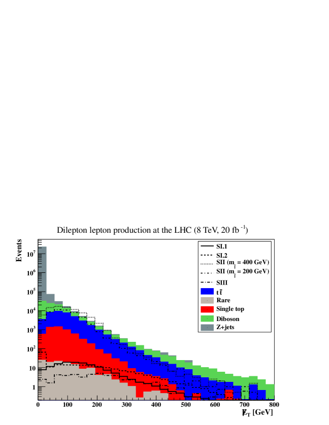
Figure 7: Missing transverse energy distribution after vetoing events with at least one $b$-tagged jet and selecting events with exactly two charged leptons. We considered 20 fb^-1 of LHC collisions at a center-of-mass energy of 8 TeV and present results for the different background contributions and for all the considered LRSUSY scenarios.

Consequently, it is tempting to impose a $Z$-veto on the invariant mass of the two leptons. However, this selection has a very low signal efficiency so that we instead make the choice of requiring a combined selection on the missing transverse energy and the transverse momentum of the leptons. In Figure 7, we present the missing transverse energy spectrum of the different contributions to the SM background together with the corresponding spectrum for the considered signal scenarios, i.e., all the four scenarios of Section 3, when the slepton mass is fixed to 400 GeV, and the scenario SII in the case where the slepton mass is set to 200 GeV. This leads us to impose $\not{E}_{T}\geq 80$ GeV, which reduces the background by a factor of about 575 and leads to the rejection of more than 99.9% of the $Z$+jets events. The surviving $Z$+jets events subsequently only contribute to 16% of the SM background, now dominated by $t\bar{t}$ events (45%) and diboson events (33%).

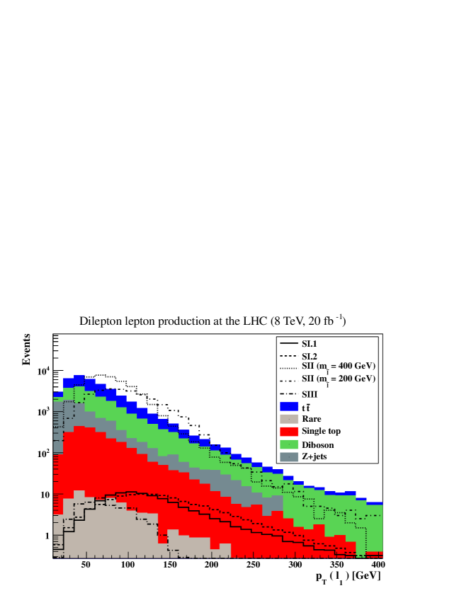
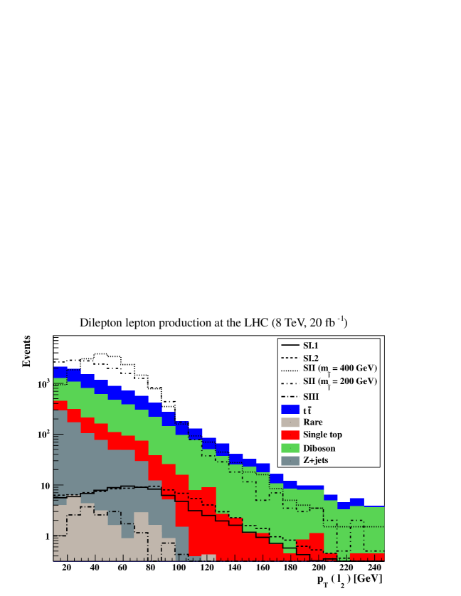
Figure 8: Transverse-momentum spectrum of the leading lepton $\ell_{1}$, after selecting events with exactly two charged leptons and no $b$-tagged jets, and at least 80 GeV of missing transverse energy. We considered 20 fb^-1 of LHC collisions at a center-of-mass energy of 8 TeV and present results for the different background contributions and for all the considered LRSUSY scenarios.

Figure 9: Transverse-momentum spectrum of the next-to-leading lepton $\ell_{2}$, after selecting events with exactly two charged leptons and no $b$-tagged jet, at least 80 GeV of missing transverse energy and a hard leading lepton with a $p_{T}$ greater than 80 GeV. We considered 20 fb^-1 of LHC collisions at a center-of-mass energy of 8 TeV and present results for the different background contributions and for all the considered LRSUSY scenarios.

In Figure 9, we present the transverse-momentum distributions of the leading lepton for both the remaining background and signal events. While scenarios of type SII are already expected to be observable, we further refine our analysis in order to try getting sensitivity to some of the other scenarios under consideration. We hence include an additional restriction on the hardest of the two identified leptons $\ell_{1}$, requiring its transverse momentum to satisfy $p_{T}(\ell_{1})\geq 80$ GeV. In addition, we impose that the next-to-leading lepton $\ell_{2}$ has to be hard, selecting events only if its $p_{T}$ is larger than 70 GeV. The effect of this last restriction can be estimated from Figure 9 where we present the $p_{T}$ distribution of the second lepton after all previous selections. Both these requirements ensure, together with our basic lepton isolation criteria, that the non-simulated multijet background contributions including fake leptons are under control (see, e.g., Ref Chatrchyan:2012oaa ).

Scenario	Signal ($S$)	Background ($B$)	$S/\sqrt{S+B}$
SI.1	$41.2\pm 6.8$	$1748.3\pm 41.7$	$0.97\pm 0.32$
SI.2	$53.9\pm 7.7$		$1.27\pm 0.36$
SII (200 GeV sleptons)	$2610\pm 56$		$39.5\pm 1.2$
SII (400 GeV sleptons)	$2686\pm 57$		$40.3\pm 1.2$
SIII	$2.6\pm 1.8$		$0.06\pm 0.08$

Table 9: Number of expected dilepton events for 20 fb^-1 of LHC collisions at a center-of-mass energy of 8 TeV, together with the associated statistical uncertainties, after applying all the selections described in the text. We present numbers of event $S$ for each of the signal scenarios introduced in Section 3 after including a NLO $K$-factor set to 1.2 and for the background ($B$). The results are then converted in terms of LHC significance to LRSUSY signals in dileptonic final states.

The number of background events is subsequently found to be comparable with the number of signal events in LRSUSY scenarios of class SII, as shown in Table 9. We also indicate in the table the expected significance for each benchmark point computed as the ratio of the number of selected signal events to the squared root of the total number of predicted events. At this stage, background consists mainly of top-antitop events (44%), diboson events (46%) and single top events in the $tW$ channel (7%). Comparing with the single lepton analysis of Section 4.2.1, we found that the SII scenarios are likely to be observed with a very strong significance for both chosen slepton mass. Unfortunately, there is still no sensitivity to the other considered scenarios.

4.2.3 Signatures with three leptons or more

The two previous analyses are only sensitive to scenarios of class SII mainly because they feature a larger neutralino and chargino pair-production cross section due to the light associated masses. When gauginos are heavier, the LHC sensitivity to the corresponding LRSUSY signals is reduced, as for our scenarios SI.1 and SI.2, and it becomes difficult to extract the few LRSUSY signal events from the overwhelming Standard Model background. We therefore focus now on a multileptonic analysis requiring at least three charged leptons. This topology has the benefit of a reduced Standard Model background so that new physics processes with low cross sections can possibly show hints in the observations.

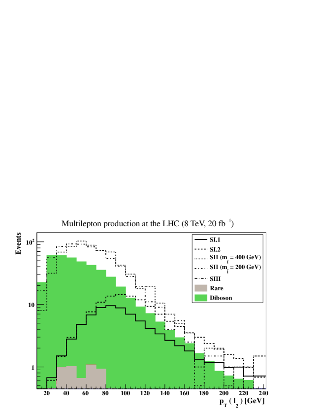
Figure 10: Transverse-momentum spectrum of the next-to-leading lepton $\ell_{2}$, after vetoing events with at least one $b$-tagged jet and selecting events with at least three charged leptons, at least 100 GeV of missing transverse energy and a hard leading lepton with a $p_{T}$ greater than 80 GeV. We considered 20 fb^-1 of LHC collisions at a center-of-mass energy of 8 TeV and present results for the different background contributions and for all the considered LRSUSY scenarios.

Scenario	Signal ($S$)	Background ($B$)	$S/\sqrt{S+B}$
SI.1	$65.4\pm 8.4$	$133.4\pm 11.5$	$4.64\pm 1.03$
SI.2	$108\pm 10$		$6.98\pm 1.09$
SII (200 GeV sleptons)	$259\pm 18$		$13.1\pm 1.3$
SII (400 GeV sleptons)	$289\pm 19$		$14.1\pm 1.3$
SIII	$\approx 0$		-

Table 10: Number of expected multilepton events (with three ore more charged leptons) for 20 fb^-1 of LHC collisions at a center-of-mass energy of 8 TeV, together with the associated statistical uncertainties, after applying all the selections described in the text. We present numbers of event $S$ for each of the signal scenarios introduced in Section 3 after including a NLO $K$-factor set to 1.2 and for the background ($B$). The results are then converted in terms of LHC significance to LRSUSY signals in multileptonic final states (with three or more charged leptons).

Signal efficiency for scenarios of class SI is found to be moderate, reaching 20%-30%, in contrast to the other scenarios for which it lies below 1%. This low value is nevertheless compensated, in the case of scenario SII, by the large cross section. As mentioned above, the Standard Model background is reduced (only about 5500 events are expected) and mainly due to diboson events (at 99.5%). In the context of the Standard Model, the charged leptons included in those events originate from a $Z$-boson or a $W$-boson leptonic decay. Therefore, we follow the same strategy as in Section 4.2.2 and, instead of vetoing events with a lepton pair compatible with a $Z$-boson or imposing a selection on the $W$-boson reconstructed transverse mass, we require a selection based on the missing transverse energy and on the transverse momentum of the two leading leptons. We hence impose that $\not{E}_{T}\geq 100$ GeV, together with the condition that the $p_{T}$ of the two leading leptons is above thresholds of $p_{T}(\ell_{1})\geq 80$ GeV and $p_{T}(\ell_{2})\geq 70$ GeV. As shown in Figure 10, where we illustrate the last selection on the transverse momentum of the next-to-leading lepton $\ell_{2}$, those simple cuts are sufficient to highlight most of the considered LRSUSY signals from the diboson background.

The results are summarized in Table 10 where we present, in addition to the Standard Model expectation after all selections, the number of signal events expected for each of the considered LRSUSY scenarios and the associated significance given as $S/\sqrt{S+B}$. It can be seen that it reaches more than $3\sigma$ in all cases, with the exception of scenario SIII since its compressed spectrum does not allow for any visible signature.

4.3 Comparison with the MSSM

We now turn to the comparison of LRSUSY signals with MSSM signals in the context of the analyses introduced in Section 4.2. Assuming the observation of excesses in events with a leptonic final state and a supersymmetric explanation for such excesses, we address the question of probing the underlying theory and investigate if it exhibits more an MSSM or LRSUSY structure. We first design MSSM scenarios with similar features as the LRSUSY benchmarks of Section 3. To this aim, we follow the procedure below.

• We start from a LRSUSY scenario and remove the neutralino and the chargino with the largest $SU(2)_{R}$ wino component.

• The two remaining LRSUSY neutralinos are identified as the two lighter neutralinos of the MSSM after neglecting their $SU(2)_{R}$ wino component. The masses are fixed to the same values in both models.

• The remaining LRSUSY chargino is identified as the lightest MSSM chargino after neglecting its possible $SU(2)_{R}$ wino component. Its mass is fixed to the same value in both models.

• We decouple all higgsinos in the MSSM.

• We then compute, by means of the FeynRules Christensen:2008py ; Duhr:2011se and ASperGe Alloul:2013fw programs, the tree-level neutralino and chargino mass matrices and calculate the soft SUSY-breaking $U(1)_{Y}$ bino and $SU(2)_{L}$ wino mass parameters $M_{1}$ and $M_{2}$ leading to the proper mass eigenvalues.

This last step also enforces the choice for the mixing parameters in the MSSM. We show the results in Table 11, giving the values found for the $M_{1}$ and $M_{2}$ parameters. We hence design three scenarios mimicking the LRSUSY scenarios SI.1, SI.2 and SII. Moreoer, we do not consider the LRSUSY scenario SIII as it is invisible at the LHC when considering leptonic final states.

Scenario	$M_{1}$ [GeV]	$M_{2}$ [GeV]	$m_{\tilde{\chi}^{0}_{1}}$ [GeV]	$m_{\tilde{\chi}^{0}_{2}}$ [GeV]	$m_{\tilde{\chi}_{1}^{+}}$ [GeV]
SI.1	270	506	270	500	500
SI.2	270	760	269	747	747
SII	112	254	111	250	250

Table 11: MSSM scenarios SI.1, SI.2 and SII equivalent to their LRSUSY counterparts of Section 3.

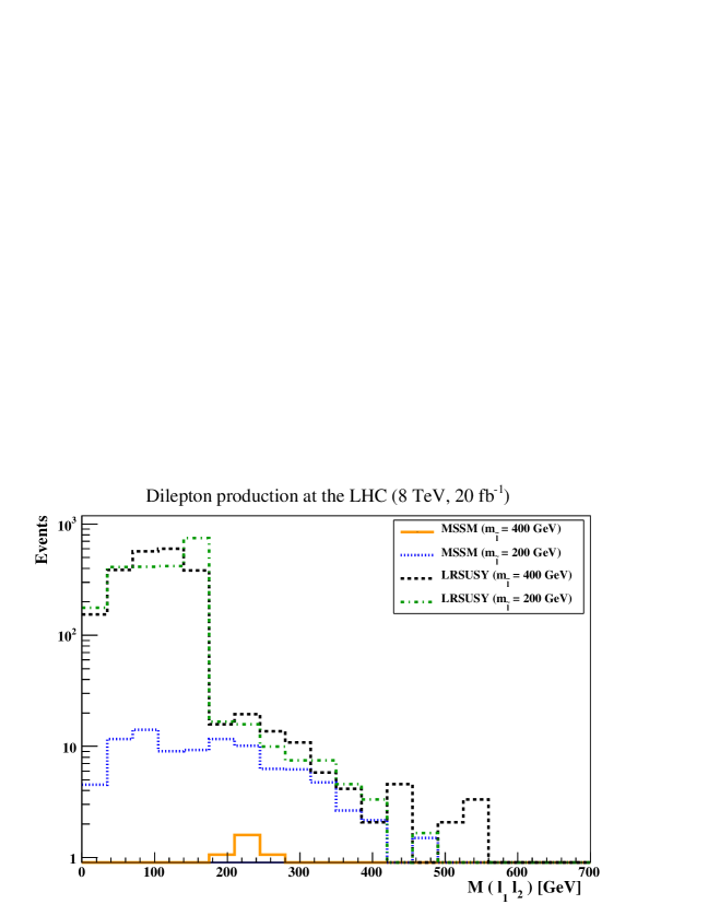
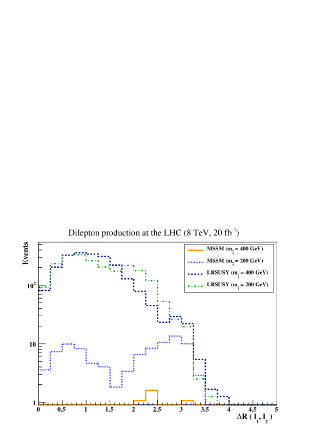
Figure 11: Invariant mass (upper panel) and angular distance (lower panel) of a dilepton pair in MSSM and LRSUSY models after selecting events with exactly two charged leptons and no $b$-tagged jet, at least 80 GeV of missing transverse energy, and two leading leptons with a $p_{T}$ greater than 80 GeV and 70 GeV, respectively. We considered 20 fb^-1 of LHC collisions at a center-of-mass energy of 8 TeV and benchmark scenarios of type SII with 200 GeV and 400 GeV sleptons.

For the sake of simplicity, we focus on the most promising channels, namely the dilepton and multilepton (with three or more final state charged leptons) analyses. After applying the selection criteria presented in Section 4.2.2 and Section 4.2.3, we investigate key distributions allowing to possibly disentangle a LRSUSY behavior from an MSSM one. Since in the dilepton case, only scenario SII leads to a signal likely to be observed, we restrain the comparison to it and show the results in Figure 11. We present invariant mass and angular distance distributions among the two leading leptons for both the LRSUSY and MSSM cases, fixing the slepton masses either to 200 GeV or to 400 GeV. We observe that very few events are expected in the case of the MSSM, in contrast to the LRSUSY one. Moreover, the shapes of the distributions are found also quite different, so that they offer a possible way to distinguish both models assuming a given supersymmetric spectrum.

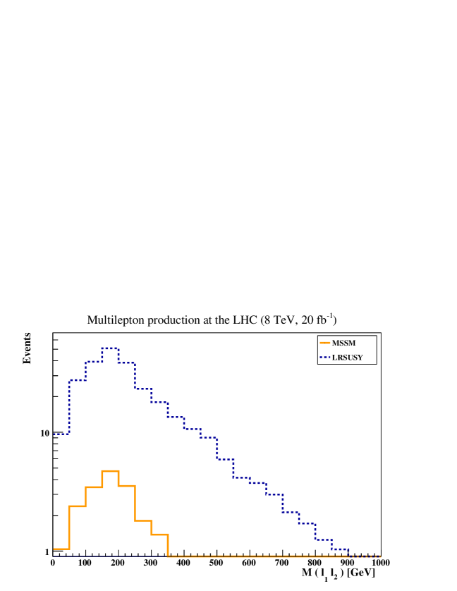
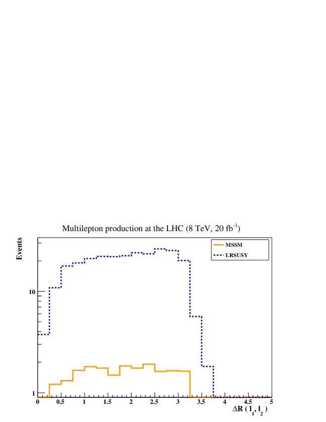
Figure 12: Invariant mass (upper panel) and angular distance (lower panel) of a dilepton pair comprised of the two leading leptons $\ell_{1}$ and $\ell_{2}$ in MSSM and LRSUSY models after selecting events with at least three charged leptons and no $b$-tagged jets, at least 100 GeV of missing transverse energy, and two leading leptons with a $p_{T}$ greater than 80 GeV and 70 GeV, respectively. We considered 20 fb^-1 of LHC collisions at a center-of-mass energy of 8 TeV and benchmark scenarios of type SI.1 with 400 GeV sleptons.

In the case of the multilepton analysis of Section 4.2.3, no signal events are expected to survive the selection strategy designed for the MSSM counterparts of our scenarios SI.2 and SII. In contrast, more than a $5\sigma$ sensitivity is expected in the LRSUSY case. For scenarios of type SI.1, lighter gaugino masses ensure that a few MSSM events can be selected. We therefore illustrate their properties in Figure 12, where we present the invariant mass (upper panel) and angular distance (lower panel) distributions of a particle pair comprised of the two leading charged leptons. As for the dilepton case, a larger number of events is expected in LRSUSY models. However, the shapes of the distributions are this time more similar. Nevertheless, if one restricts the spectra to their higher value bins containing many LRSUSY events but very few MSSM events, this analysis again offers a possible way to distinguish both cases.

5 Conclusions

In this work we explored the possibility that the associated production of charginos and neutralinos can be observed at the LHC. We choose to work in a supersymmetric scenario where their production is likely to be enhanced, in a model where the gauge symmetry is left-right symmetric, based on the $SU(3)_{c}\times SU(2)_{L}\times SU(2)_{R}\times U(1)_{B-L}$ group. This model has twelve neutralinos (including two additional gauginos) and six (singly-charged) charginos (including an additional gaugino). In comparison the MSSM has four neutralinos and two charginos. We present a complete description of the model, and follow this by a choice of benchmark scenarios, chosen to highlight different mixing schemes and hierarchies among chargino and neutralino states. After making some general observations about the patterns of chargino and neutralino decays in LRSUSY, and possible distinguishing signs from similar decays in the MSSM, we present complete production and decay calculations for the benchmark scenarios, classified according to the number of leptons in the final state. We proceed to event simulations, where we include the Standard Model backgrounds. We devise methods to increase the signal to background significance, specifically for each one-lepton, two-lepton and three-or-more-lepton final states. We complement our analysis by a simulation of events consistent with our benchmark scenarios in the MSSM context (as much as possible).

Several general features emerge from our analysis. First, for most of the parameter space, with the exception of one scenario featuring large gaugino mass splittings, the single lepton signal would not be visible at the LHC, as it is completely swamped by the background, even after stringent requirements on the missing transverse energy and transverse momentum of the lepton. Imposing further selection would then suppress both signal and background. Second, two- and three-lepton signals are however visible above the background, especially in kinematical distributions associated with the leading and next-to-leading leptons. Interesting, the most promising scenario is the one in which the LSP is a mixed state, a bino with a significant ${\tilde{W}}_{R}^{0}$ component, while the next-to-lightest superpartner is pure left-handed wino. This benchmark scenario raises above backgrounds after applying the complete designed selection strategies, yielding visible LRSUSY signal at the LHC. And third, the number of events expected in LRSUSY scenarios of type SII is significantly above the expectations (one to two orders of magnitude, and different in shape) for the same events in a similar scenario in the MSSM in the two-lepton final state, but less so in the three-or-more-leptons, yielding a clear distinguishing signal from left-right supersymmetric models.

In a nutshell, enhanced production and decays of chargino and neutralino appear to be very promising signatures of supersymmetric models with extended gauge sectors, and in particular, for the left-right supersymmetric model, if these particles are light. These events complete favorably, and are complementary to, signals from the production and decays of doubly-charged higgsinos as means to test for left-right supersymmetry.

Appendix A Conventions

In this Section, we recall some basic features of Lie algebras in order to fix the notations and correctly define the various relative signs which appear in the model described in Section 2. Denoting $T_{a}$ the matrices of a unitary representation ${\cal R}$ of a given Lie algebra $\mathfrak{g}$, it is well known that the matrices $-T^{t}$, $-T^{\star}$ and $T^{\dagger}$, i.e., the transposed, complex conjugate and Hermitian conjugate matrices of $T$, span also representations of the Lie algebra $\mathfrak{g}$. The representation spanned by the matrices $-T_{a}^{t}$ is called the dual representation ${\cal R}^{\ast}$, the one spanned by the matrices $-T_{a}^{\star}$ the complex conjugate representation $\overline{{\cal R}}$ and the one spanned by the matrices $T^{\dagger}_{a}$ the dual of the complex conjugate representation $\overline{{\cal R}}^{*}$.

However, it may happen that some of these four representations are isomorphic. As an example, for $SU(2)$, if we denote $\utilde{\bf 2}$ the two-dimensional (fundamental) representation spanned by the Pauli matrices $\frac{1}{2}\sigma_{i}$, it turns out that we get the isomorphism $\utilde{\bf 2}\cong\utilde{\bf 2}^{*}\cong\utilde{\bf\bar{2}}$, since

$$-\sigma^{t}_{i}=\sigma_{2}\ \sigma_{i}\ \sigma_{2}^{-1}\quad\text{and}\quad-\sigma^{\star}_{i}=\sigma_{2}\ \sigma_{i}\ \sigma_{2}^{-1}\ .$$ (47)

The first of these two isomorphisms allows to raise or lower the two-dimensional indices by the mean of the invariant $SU(2)$ tensors $\varepsilon_{ij}$ and $\varepsilon^{ij}$ defined by $\varepsilon_{12}=-\varepsilon_{21}=-\varepsilon^{12}=\varepsilon^{21}=1$. Hence, for a field $\psi^{i}$ lying in the $\utilde{\bf 2}$ representation,

$$\psi_{i}=\varepsilon_{ij}\ \psi^{j}\quad\text{and}\quad\psi^{i}=\varepsilon^{ij}\ \psi_{j}\ .$$ (48)

In the case of $SU(3)$, we similarly get, for the three-dimensional representations, the relation $\utilde{\bf 3}^{*}\cong\utilde{\bf\bar{3}}$.

In this paper, we denote by $i$ and $i^{\prime}$ typical indices of the two-dimensional representation of $SU(2)_{L}$ and $SU(2)_{R}$, respectively, while we associate to the three-dimensional representation of $SU(3)_{c}$ indices labeled by $m$.

Appendix B Gauge boson mass matrices

We can extract the gauge boson mass matrices from the Higgs field kinetic terms,

$$\begin{split}M^{2}_{V^{0}}=&\ \begin{pmatrix}\frac{1}{4}g_{L}^{2}\big{(}4v_{L}^{2}\!+\!v^{2}\!+\!v^{\prime 2}\big{)}&-\frac{1}{4}g_{L}g_{R}\big{(}v^{2}+v^{\prime 2}\big{)}&-{\hat{g}}g_{L}v_{L}^{2}\\ -\frac{1}{4}g_{L}g_{R}\big{(}v^{2}+v^{\prime 2}\big{)}&\frac{1}{4}g_{R}^{2}\big{(}4v_{R}^{2}\!+\!v^{2}\!+\!v^{\prime 2}\big{)}&-{\hat{g}}g_{R}v_{R}^{2}\\ -{\hat{g}}g_{L}v_{L}^{2}&-{\hat{g}}g_{R}v_{R}^{2}&{\hat{g}}^{2}\big{(}v_{L}^{2}+v_{R}^{2}\big{)}\\ \end{pmatrix}\ ,\\ M^{2}_{V^{\pm}}=&\ \begin{pmatrix}\frac{1}{4}g_{L}^{2}\big{(}2v_{L}^{2}\!+\!v^{2}\!+\!v^{\prime 2}\big{)}&-\frac{1}{2}g_{L}g_{R}(vv^{\prime})^{\ast}\\ -\frac{1}{2}g_{L}g_{R}(vv^{\prime})&\frac{1}{4}g_{R}^{2}\big{(}2v_{R}^{2}\!+\!v^{2}\!+\!v^{\prime 2}\big{)}\\ \end{pmatrix}\ ,\end{split}$$ (49)

where we have introduced the abbreviations

$$\begin{split}&\ v_{L}^{2}=v_{1L}^{2}+v_{2L}^{2}\ ,\quad v_{R}^{2}=v_{1R}^{2}+v_{2R}^{2}\ ,\\ &\ v^{2}=v_{1}^{2}+v_{2}^{2}\ ,\quad v^{\prime 2}=v_{1}^{\prime 2}+v_{2}^{\prime 2}\ ,\quad vv^{\prime}=v_{1}v_{1}^{\prime}e^{i\alpha_{1}}+v_{2}v_{2}^{\prime}e^{i\alpha_{2}}\ .\end{split}$$ (50)

In the limit of the vev hierarchy of Eq. (17), the mass matrix of the neutral gauge bosons, usually diagonalized with the help of an orthogonal $3\times 3$ matrix $U_{g}^{0}$, is diagonalized through two independent rotations of angles $\theta_{W}$ and $\phi$. This follows the model breaking pattern. After the breaking of the $SU(2)_{R}\times U(1)_{B-L}$, the neutral $W_{R\mu}^{3}$ and $\hat{B}_{\mu}$ fields mix to a massless state, which will be identified to the hypercharge field $B^{\prime}_{\mu}$, and a massive ${Z^{\prime}}$-boson, which will decouple from the breakdown process. When the electroweak symmetry is eventually broken at a lower scale to electromagnetism, the hypercharge field and the neutral $W_{L\mu}^{3}$ field then mix to a massless state identified to the photon $A_{\mu}$ and to a massive state, the $Z$-boson. The mixing matrix takes a simple form,

$$\begin{split}\begin{pmatrix}Z_{\mu}\\ A_{\mu}\\ {Z^{\prime}}_{\mu}\end{pmatrix}=&\ \begin{pmatrix}{\cos\theta_{W}}&-{\sin\theta_{W}}\sin\phi&-{\sin\theta_{W}}\cos\phi\\ {\sin\theta_{W}}&{\cos\theta_{W}}\sin\phi&{\cos\theta_{W}}\cos\phi\\ 0&\cos\phi&-\sin\phi\\ \end{pmatrix}\begin{pmatrix}W_{L\mu}^{3}\\ W_{R\mu}^{3}\\ \hat{B}_{\mu}\end{pmatrix}\\ =&\ \begin{pmatrix}\frac{e}{g_{Y}}&-\frac{e\ g_{Y}}{g_{L}\ g_{R}}&-\frac{e\ g_{Y}}{g_{L}\ {\hat{g}}}\\ \frac{e}{g_{L}}&\frac{e}{g_{R}}&\frac{e}{{\hat{g}}}\\ 0&\frac{g_{Y}}{{\hat{g}}}&-\frac{g_{Y}}{g_{R}}\\ \end{pmatrix}\begin{pmatrix}W_{L\mu}^{3}\\ W_{R\mu}^{3}\\ \hat{B}_{\mu}\end{pmatrix}\ ,\end{split}$$ (51)

where in the last line, we have expressed the mixing angles as functions of the electromagnetic coupling constant $e$, the hypercharge coupling constant $g_{Y}$ and the unbroken gauge group coupling constants $g_{L}$, $g_{R}$ and ${\hat{g}}$. The physical masses are given by

$$\begin{split}m_{Z^{\prime}}^{2}=&\ v_{R}^{2}({\hat{g}}^{2}+g_{R}^{2})=\frac{g_{R}^{2}}{\cos\phi^{2}}v_{R}^{2}\ ,\\ m_{Z}^{2}=&\ \frac{1}{4}\Big{[}g_{L}^{2}+\sin\phi^{2}g_{R}^{2}\Big{]}v^{2}=\frac{g_{L}^{2}}{4\cos^{2}\theta_{W}}v^{2}\ ,\end{split}$$ (52)

and the photon stay massless. We have also the following relations, linking the mixing angles to the coupling constants,

$$\begin{split}&\ \cos\phi=\frac{g_{R}}{\sqrt{g_{R}^{2}+{\hat{g}}^{2}}}\ ,\quad\sin\phi=\frac{{\hat{g}}}{\sqrt{g_{R}^{2}+{\hat{g}}^{2}}},\quad\\ &\ {\cos\theta_{W}}=\frac{g_{L}}{\sqrt{g_{R}^{2}\sin\phi^{2}+g_{L}^{2}}}\ ,\quad{\sin\theta_{W}}=\frac{g_{R}\sin\phi}{\sqrt{g_{R}^{2}\sin\phi^{2}+g_{L}^{2}}}\ .\end{split}$$ (53)

Turning to the charged sector, the mass matrix is usually diagonalized by a $2\times 2$ unitary matrix $U_{g}^{\pm}$. However, in the approximation of Eq. (17), $U_{g}^{\pm}$ tends to the identity matrix, the mass of the two eigenstates being simply

$$m_{W}^{2}=\frac{g_{L}^{2}}{4}v^{2}\quad\text{and}\quad m_{W^{\prime}}^{2}=\frac{1}{2}g_{R}^{2}v_{R}^{2}\ .$$ (54)

References

- (1) A. G. Clark [ATLAS and CMS Collaborations], arXiv:1011.6572 [hep-ex]; in the Proceedings of the Hadron Collider Physics Symposium 2010: HCP 2010.
- (2) https://twiki.cern.ch/twiki/bin/view/AtlasPublic/SupersymmetryPublicResults.
- (3) https://twiki.cern.ch/twiki/bin/view/CMSPublic/PhysicsResultsSUS.
- (4) J. C. Pati and A. Salam, Phys. Rev. D 10 (1974) 275 [Erratum-ibid. D 11 (1975) 703].
- (5) R. N. Mohapatra and J. C. Pati, Phys. Rev. D 11 (1975) 566.
- (6) R. N. Mohapatra and J. C. Pati, Phys. Rev. D 11 (1975) 2558.
- (7) G. Senjanovic and R. N. Mohapatra, Phys. Rev. D 12 (1975) 1502.
- (8) R. N. Mohapatra, F. E. Paige and D. P. Sidhu, Phys. Rev. D 17 (1978) 2462.
- (9) G. Senjanovic, Nucl. Phys. B 153 (1979) 334.
- (10) R. N. Mohapatra and G. Senjanovic, Phys. Rev. Lett. 44 (1980) 912.
- (11) R. N. Mohapatra and A. Rasin, Phys. Rev. Lett. 76 (1996) 3490.
- (12) R. N. Mohapatra and A. Rasin, Phys. Rev. D 54 (1996) 5835.
- (13) R. Kuchimanchi, Phys. Rev. Lett. 76 (1996) 3486.
- (14) R. Kuchimanchi and R. N. Mohapatra, Phys. Rev. D 48 (1993) 4352.
- (15) K. S. Babu, S. M. Barr, Phys. Rev. D48 (1993) 5354.
- (16) K. S. Babu, S. M. Barr, Phys. Rev. D50 (1994) 3529.
- (17) M. Frank, H. Hamidian, K. Puolamaki, Phys. Lett. B456 (1999) 179.
- (18) M. Frank, H. Hamidian, K. Puolamaki, Phys. Rev. D60 (1999) 095011.
- (19) R. N. Mohapatra, hep-ph/9801235, and references therein.
- (20) R. M. Francis, M. Frank and C. S. Kalman, Phys. Rev. D 43 (1991) 2369.
- (21) K. Huitu, J. Maalampi and M. Raidal, Phys. Lett. B 328 (1994) 60.
- (22) K. Huitu, J. Maalampi and M. Raidal, Nucl. Phys. B 420 (1994) 449.
- (23) A. G. Akeroyd, C. -W. Chiang, N. Gaur, JHEP 1011 (2010) 005.
- (24) A. G. Akeroyd, C. -W. Chiang, Phys. Rev. D80 (2009) 113010.
- (25) Y. -L. Ma, Phys. Rev. D79 (2009) 033014.
- (26) P. Ren, Z. -z. Xing, Phys. Lett. B666 (2008) 48.
- (27) C. -S. Chen, C. -Q. Geng, D. V. Zhuridov, Eur. Phys. J. C60 (2009) 119.
- (28) T. Han, B. Mukhopadhyaya, Z. Si et al., Phys. Rev. D76 (2007) 075013.
- (29) B. Mukhopadhyaya, S. K. Rai, Phys. Lett. B633 (2006) 519.
- (30) G. Azuelos, K. Benslama, J. Ferland, J. Phys. G G32 (2006) 73.
- (31) M. Muhlleitner, M. Spira, Phys. Rev. D68 (2003) 117701.
- (32) S. Godfrey, P. Kalyniak, N. Romanenko, Phys. Rev. D65 (2002) 033009.
- (33) B. Dutta, R. N. Mohapatra, Phys. Rev. D59 (1999) 015018.
- (34) K. Huitu, J. Maalampi, A. Pietila et al., Nucl. Phys. B487 (1997) 27.
- (35) A. Alloul, M. Frank, B. Fuks and M. R. de Traubenberg, arXiv:1307.1711 [hep-ph].
- (36) Z. Chacko and R. N. Mohapatra, Phys. Rev. D 58 (1998) 015003.
- (37) M. Raidal, P. M. Zerwas, Eur. Phys. J. C8 (1999) 479.
- (38) D. A. Demir, M. Frank, D. K. Ghosh et al., Phys. Rev. D79 (2009) 095006.
- (39) D. A. Demir, M. Frank, K. Huitu et al., Phys. Rev. D78 (2008) 035013.
- (40) M. Frank, K. Huitu, S. K. Rai, Phys. Rev. D77 (2008) 015006.
- (41) M. Frank, A. Hayreter and I. Turan, Phys. Rev. D 83 (2011) 035001.
- (42) J. Yamaoka [CDF and D0 Collaboration], PoS EPS -HEP2009 (2009) 239.
- (43) Y. Li and A. Nomerotski, arXiv:1007.0698 [physics.ins-det], in the Proceedings of International Linear Collider Workshop 2010 (LCWS10 & ICL10).
- (44) D. Kafer, J. List and T. Suehara, arXiv:0901.4958 [hep-ex], in the Proceedings of International Linear Collider Workshop 2010 (LCWS10 & ICL10).
- (45) K. Huitu, J. Laamanen, P. N. Pandita et al., Phys. Rev. D82 (2010) 115003.
- (46) G. Aad et al. [ATLAS Collaboration], Phys. Lett. B 718 (2013) 879.
- (47) G. Aad et al. [ATLAS Collaboration], Phys. Lett. B 718 (2013) 841.
- (48) [ATLAS Collaboration], ATLAS-CONF-2012-041.
- (49) G. Aad et al. [ATLAS Collaboration], Phys. Rev. Lett. 108 (2012) 261804.
- (50) S. Chatrchyan et al. [CMS Collaboration], JHEP 1211 (2012) 147.
- (51) S. Chatrchyan et al. [CMS Collaboration], JHEP 1206 (2012) 169.
- (52) S. Chatrchyan et al. [CMS Collaboration], Phys. Lett. B 704 (2011) 411.
- (53) [CMS Collaboration], CMS-PAS-SUS-12-022.
- (54) K. S. Babu and R. N. Mohapatra, Phys. Lett. B 668 (2008) 404.
- (55) M. Frank and B. Korutlu, Phys. Rev. D 83 (2011) 073007.
- (56) C. S. Aulakh, A. Melfo, A. Rasin and G. Senjanovic, Phys. Rev. D 58 (1998) 115007.
- (57) C. S. Aulakh, K. Benakli and G. Senjanovic, Phys. Rev. Lett. 79 (1997) 2188.
- (58) K. S. Babu, B. Dutta and R. N. Mohapatra, Phys. Rev. D 60 (1999) 095004.
- (59) D. Borah, J. Mod. Phys. 3 (2012) 1097.
- (60) S. -L. Chen, D. K. Ghosh, R. N. Mohapatra and Y. Zhang, JHEP 1102 (2011) 036.
- (61) D. Borah and U. A. Yajnik, Phys. Rev. D 83 (2011) 095004.
- (62) B. Dutta, R. N. Mohapatra and D. J. Muller, Phys. Rev. D 60 (1999) 095005.
- (63) K. S. Babu, B. Dutta and R. N. Mohapatra, Phys. Rev. D 65 (2002) 016005.
- (64) P. Fileviez Perez and S. Spinner, Phys. Lett. B 673 (2009) 251.
- (65) A. Vicente, J. Phys. Conf. Ser. 259 (2010) 012065.
- (66) M. C. Rodriguez, arXiv:0710.1100 [hep-ph].
- (67) Y. .B. Zeldovich, I. Y. .Kobzarev and L. B. Okun, Zh. Eksp. Teor. Fiz. 67 (1974) 3 [Sov. Phys. JETP 40 (1974) 1].
- (68) A. Vilenkin, Phys. Rept. 121 (1985) 263.
- (69) J. Beringer et al. [Particle Data Group Collaboration], Phys. Rev. D 86 (2012) 010001.
- (70) L. E. Ibanez, Phys. Lett. B 137 (1984) 160.
- (71) J. S. Hagelin, G. L. Kane and S. Raby, Nucl. Phys. B 241 (1984) 638.
- (72) T. Falk, K. A. Olive and M. Srednicki, Phys. Lett. B 339 (1994) 248.
- (73) C. Arina, arXiv:0805.1991 [hep-ph].
- (74) D. A. Demir, L. L. Everett, M. Frank, L. Selbuz and I. Turan, Phys. Rev. D 81 (2010) 035019.
- (75) J. Alwall, M. Herquet, F. Maltoni, O. Mattelaer and T. Stelzer, JHEP 1106 (2011) 128.
- (76) J. Pumplin, D. R. Stump, J. Huston, H. L. Lai, P. M. Nadolsky and W. K. Tung, JHEP 0207 (2002) 012.
- (77) C. Degrande, C. Duhr, B. Fuks, D. Grellscheid, O. Mattelaer and T. Reiter, Comput. Phys. Commun. 183 (2012) 1201.
- (78) N. D. Christensen and C. Duhr, Comput. Phys. Commun. 180 (2009) 1614.
- (79) N. D. Christensen, P. de Aquino, C. Degrande, C. Duhr, B. Fuks, M. Herquet, F. Maltoni and S. Schumann, Eur. Phys. J. C 71 (2011) 1541.
- (80) N. D. Christensen, C. Duhr, B. Fuks, J. Reuter and C. Speckner, Eur. Phys. J. C 72 (2012) 1990.
- (81) C. Duhr and B. Fuks, Comput. Phys. Commun. 182 (2011) 2404.
- (82) B. Fuks, Int. J. Mod. Phys. A 27 (2012) 1230007.
- (83) A. Alloul, J. D’Hondt, K. De Causmaecker, B. Fuks and M. Rausch de Traubenberg, Eur. Phys. J. C 73 (2013) 2325.
- (84) W. Beenakker, M. Klasen, M. Kramer, T. Plehn, M. Spira and P. M. Zerwas, Phys. Rev. Lett. 83 (1999) 3780 [Erratum-ibid. 100 (2008) 029901].
- (85) J. Debove, B. Fuks and M. Klasen, Nucl. Phys. B 842 (2011) 51.
- (86) J. Debove, B. Fuks and M. Klasen, Phys. Lett. B 688 (2010) 208.
- (87) J. Debove, B. Fuks and M. Klasen, Nucl. Phys. B 849 (2011) 64.
- (88) T. Sjostrand, S. Mrenna and P. Z. Skands, JHEP 0605 (2006) 026.
- (89) T. Sjostrand, S. Mrenna and P. Z. Skands, Comput. Phys. Commun. 178 (2008) 852.
- (90) M. L. Mangano, M. Moretti, F. Piccinini and M. Treccani, JHEP 0701 (2007) 013.
- (91) J. Alwall, S. de Visscher and F. Maltoni, JHEP 0902 (2009) 017.
- (92) E. Conte, B. Fuks and G. Serret, Comput. Phys. Commun. 184 (2013) 222.
- (93) H. -L. Lai, M. Guzzi, J. Huston, Z. Li, P. M. Nadolsky, J. Pumplin and C. -P. Yuan, Phys. Rev. D 82 (2010) 074024.
- (94) R. Gavin, Y. Li, F. Petriello and S. Quackenbush, Comput. Phys. Commun. 182 (2011) 2388.
- (95) R. Gavin, Y. Li, F. Petriello and S. Quackenbush, Comput. Phys. Commun. 184 (2013) 208.
- (96) M. Aliev, H. Lacker, U. Langenfeld, S. Moch, P. Uwer and M. Wiedermann, Comput. Phys. Commun. 182 (2011) 1034.
- (97) N. Kidonakis, arXiv:1205.3453 [hep-ph].
- (98) J. M. Campbell and R. K. Ellis, Phys. Rev. D 60 (1999) 113006.
- (99) J. M. Campbell, R. K. Ellis and C. Williams, JHEP 1107 (2011) 018.
- (100) J. M. Campbell and R. K. Ellis, JHEP 1207 (2012) 05.2
- (101) G. Aad et al. [ATLAS Collaboration], Eur. Phys. J. C 72 (2012) 2083.
- (102) S. Chatrchyan et al. [CMS Collaboration], Phys. Lett. B 720 (2013) 63.
- (103) M. Cacciari and G. P. Salam, Phys. Lett. B 641 (2006) 57.
- (104) M. Cacciari, G. P. Salam and G. Soyez, Eur. Phys. J. C 72 (2012) 1896.
- (105) M. Cacciari, G. P. Salam and G. Soyez, JHEP 0804 (2008) 063.