The University of Manchester, Manchester, M13 9PL, U.K.
Constraining MPI models using and recent Tevatron and LHC Underlying Event data
Abstract
We review the modelling of multiple interactions in the event generator Herwig++ and study implications of recent tuning efforts to Tevatron and LHC data. It is often said that measurements of the effective cross section for double-parton scattering, , are in contradiction with models of the final state of multi-parton interactions, but we show that the Herwig++ model is consistent with both and gives stable predictions for underlying event observables at 14 .
1 Introduction
In QCD, high momentum-transfer reactions in hadron-hadron collisions are understood as the consequence of high momentum-transfer scattering or annihilation-production processes between the partonic consituents of the hadrons. Although the hadronic structure is complicated and impossible to predict at present, the factorisation theorems of QCD predict that, for sufficiently inclusive cross sections, this complication factorises into universal (process-independent but hadron-dependent) parton distribution functions, convoluted with (process-dependent but hadron-independent) partonic cross sections. Thus, the hard cross section is seen as the consequence of one parton from each hadron interacting perturbatively.
However, in seeking to understand and predict the final states of individual hadronic collisions, one is interested in more exclusive observables, which cannot be described in this purely factorised way. One talks of the underlying event, the rest of the event that accompanies the products of a hard collision, or of soft inclusive events, hadron collisions in which no hard collision occurred. Since the pioneering work of Sjöstrand and van Zijl Sjostrand:1987su , the importance of multi-parton interactions (MPIs) has been recognised in describing both underlying events and soft inclusive events in terms of multiple parton-parton interactions within a single hadron-hadron collision. One pictures, on the Lorentz-contracted time-scale of a collision, each of the hadrons to be a frozen disc of partons, with individual partons from one interacting with the other locally and independently. Although other approaches have been tried Marchesini:1988hj , MPIs are now firmly established as the primary source of underlying event activity, particularly at the high energies achieved by the Tevatron and LHC, and are the basis of all models in current use for LHC physics.
MPIs contribute to the underlying event and soft inclusive event activity in two ways. Firstly, additional scatters can produce additional semi-soft partons throughout the event, directly resulting in additional jet (sometimes called mini-jet) activity, contributing to the energy- and hadron-flow both within hard final-state jets and between jets. Secondly, the colour structure of QCD is such that partonic scattering is dominated by octet colour-exchange. Hence partonic scattering, whether hard, semi-soft, or so soft that it does not produce any observable jet activity, generally involves a colour exchange between the two hadrons and hence soft hadron production at all rapidities in the event. The contribution of these two mechanisms means that there is a considerable interplay between the model parameters that describe the purely-MPI parts of the model, like the distribution of partons across the face of the hadron (the “matter distribution”), and those that describe the hadronisation of the final state, like the string- or cluster-model parameters, or parameters that describe colour deconnections, reconnections and interconnections between the different coloured systems resulting from different partonic scatters. Tuning one part of the model without the other becomes effectively meaningless and a given set of MPI model parameters should only be interpreted in the context of the other model parameters with which they were tuned111MPI models typically use inclusive pdf sets to guide their multi-parton distribution function models and the same comment applies there: a given set of MPI model parameters should be linked with the pdf set with which they were tuned..
Of course, to get a deeper understanding of MPIs and to separate the two aspects of their influence on final states, one would like to make a more direct measurement of double-parton events in which two (or more) independent parton-parton scatters are clearly identified. This is made very difficult by the fact that the double-parton scattering cross sections are largest for soft jets for which higher-order and non-perturbative corrections are large and the jet distributions are only quite weakly correlated with the underlying parton distributions. The principle behind all pre-LHC measurements is to use dijet or photon+jet pairs, which, in the MPI model at the partonic level, produce two back-to-back pairs each independently flat in azimuth, whereas the background from a single partonic event is strongly peaked. The more recent ATLAS measurement used W production and one dijet scatter, while future studies of events promise almost background-free measurements.
The measurements of double-parton scattering are typically phrased in terms of an effective cross section parameter, , defined as follows. One measures the cross sections for events that contain scatters of given types or , and , and of events that contain scatters of both types and , . is then defined through222If and are indistinguishable, as in 4-jet production, a statistical factor of must be inserted.
| (1) |
In the case that are inclusive cross sections, is independent of and .
A first estimate of was made by the AFS experiment Akesson:1986iv , followed by an unsuccessful search by UA2 Alitti:1991rd and a first Tevatron measurement by CDF Abe:1993rv , but the first precise measurements were made by the Tevatron experiments Abe:1997xk ; Abazov:2009gc . First LHC measurements have been made by LHCb Aaij:2011yc ; Aaij:2012dz and ATLAS Aad:2013bjm . We review these results below. Within the experimental uncertainties, there is no indication that is energy dependent and we quote an energy-independent average of
| (2) |
Within MPI models, the value of is closely related to the matter distribution. In fact, having fixed the parameters of a given MPI model, one can make an unambiguous prediction of . Within various different tunes of various different models, one obtains values in the range 20 to 40 mb. For example:
-
•
Herwig++ tune UE-EE-4-CTEQ6L1 Gieseke:2011xy ; Gieseke:2011na gives = 25.4 mb,
-
•
Herwig++ tune UE-EE-4 Gieseke:2011xy ; Gieseke:2011na gives = 30.9 mb,
-
•
Herwig++ tune UE-EE-SCR-CTEQ6L1 Gieseke:2012ft ; Arnold:2012fq gives = 22.8 mb,
-
•
Pythia 8 tune 4C Corke:2010yf ; torbjorn gives = 33.7 mb, and
-
•
Pythia 6 with various tunes (D6T, Z1, Perugia Skands:2009zm ; paolo ) gives values between 20 and 30 mb.
These values are all clearly above the experimental value, a fact that has been used to argue that the Monte Carlo MPI models are oversimplified and should be improved, for example by including -dependence Strikman:2011cx ; Frankfurt:2010ea ; Corke:2011yy or -dependence Blok:2013bpa .
In this paper, we explore the interplay between the model parameters by taking a different approach. Rather than tuning the parameters to the final-state data, fixing them at their best-fit values and comparing the prediction of with data, we instead include the value of and its experimental uncertainty as one of the pieces of data that we fit to. Within the fitting framework we can then explore whether there is a tension between and the final-state data and the extent to which we can find a set of model parameters that describe both well.
This approach is mandated by the “Summary of the Workshop on Multi-Parton Interactions (MPI) 2012” Abramowicz:2013iva whose “to do list” for MPI and Monte Carlo development starts with “The value of should serve as a constraint on the Monte Carlo models since the recent tunes of MPI models to the LHC data predict its value to be between 25–42 mb”.
We will also study the predictions of our fits for the extrapolation to 14 TeV. The remainder of this paper is set out as follows. In Sect. 2, we will set out the particular variant of MPI model that we use, as implemented in Herwig++. In Sect. 3 we briefly review the experimental measurements of and the constraint they impose on the overlap function in our model. In Sect. 4 we discuss the tuning of our model parameters to the value of and the underlying event data from CDF and ATLAS and show the extrapolation of the tunes to 14 . In Sect. 5 we make some concluding remarks and in Appendix A we show and discuss some more detailed technical aspects of our tunes.
2 MPI model
The MPI model used in Herwig++ Butterworth:1996zw ; Borozan:2002fk ; Bahr:2008dy ; Bahr:2008pv has been reviewed several times. Our intention here is not to review it again, but just to provide enough background to set our discussion of the tuning of its parameters in context.
The model is formulated in impact parameter space. At fixed impact parameter, multiple parton scatterings are assumed to be independent. Parton-parton scatterings are divided into soft and hard by a parameter , which is one of the main tuning parameters in our model. Above , scatters are assumed to be perturbative, and take place according to leading order QCD matrix elements convoluted with inclusive pdfs and a matter distribution ,
| (3) |
where
| (4) |
is the Fourier transform of the electromagnetic form factor, giving
| (5) |
with the modified Bessel function of the th kind. The parameter appearing in is another of the main tuning parameters and plays the role of an effective inverse proton radius. Note that , and therefore also , is normalised to unity. We allow the value of to vary with energy according to
| (6) |
and, in fact, it is and that we fit to data, with .
Below , scatters are assumed to be non-perturbative, with “Gaussian” transverse momentum distribution and valence-like longitudinal momentum distribution. The matter distribution is assumed to have the same form as above, but we allow it to have a different value. We therefore label it as . We call the transverse momentum distribution “Gaussian”, because once the parameters are fitted to data, it turns out that the width of the Gaussian is imaginary and hence the distribution in transverse momentum is actually peaked at and small at very small .
The inelastic hadron-hadron cross section serves as a constraint on the parameters, given by
| (7) |
as does the inelastic slope parameter. The differential parton-parton cross section is required to be continuous at . Thus, given the parameters and , the values of , and its Gaussian width are fixed.
The probability distribution of number of scatters is Poissonian at a given value of impact parameter, but the distribution over impact parameter gives a considerably longer than Poissonian tail. The number of soft and hard scatters is chosen according to this distribution and generated according to their respective distributions. Each hard scatter is evolved back to the incoming hadron according to the standard parton shower machinery. Energy-momentum conservation is imposed at this stage by rejecting any scatters that take the total energy extracted from the hadron above its total energy. The individual scatters are either colour connected with each other in a random (i.e. uncorrelated with their hardness) sequence, or disconnected from other scatters, with probability . A colour reconnection model, described in detail in Ref. Gieseke:2012ft , with reconnection probability is applied. The parameters we tune to data are therefore and from Eq. (6), , and .
Within this model, the probability of perturbative scatters of type and of type is
| (8) |
The inclusive cross section is then
| (9) |
so that
| (10) |
That is, within our model, a measurement of translates directly into a measurement of .
3 Measurements of
In this section we briefly review the experimental measurements of made to date.
The first evidence for double parton scattering was obtained by the AFS collaboration Akesson:1986iv from 4-jet events in collisions at . They extracted a value of , without quoting an uncertainty. It is interesting to note that they stated their expectation as .
The UA2 collaboration performed a search for double parton scattering Alitti:1991rd in 4-jet events in collisions at but only set a limit, at 95% confidence level. They stated their expectation as .
The CDF collaboration made a first measurement from 4-jet events in collisions at Abe:1993rv quoting a value of (stating their expectation as ).
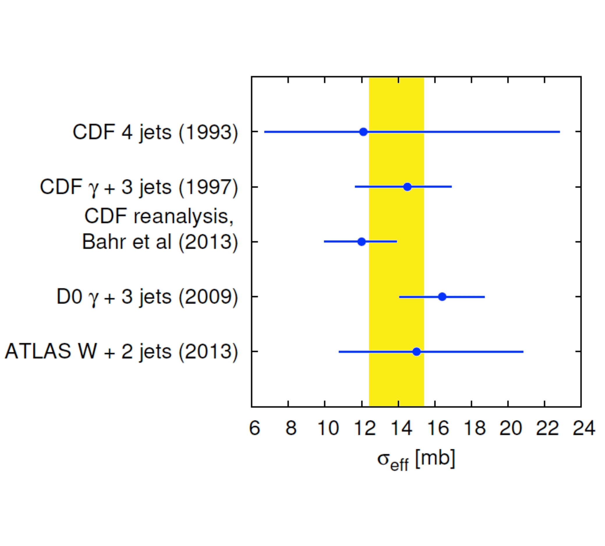
Four years later, CDF were able to make a much more precise measurement, from -jet events Abe:1997xk . They extracted a value of
| (11) |
with their expectation stated as . However, as first pointed out by Treleani Treleani:2007gi , this CDF measurement used a non-standard definition of the double-parton scattering cross section that makes the value of dependent on the individual scattering cross sections. Based on a theoretically-pure (parton-level) analysis, Treleani estimated the inclusive (process independent) value as
| (12) |
This result would be correct under the assumption that CDF were able to uniquely identify and count the number of scatters in an event, which is certainly not the case. In our recent paper, Ref. Bahr:2013gkj , we re-analyzed CDF’s event definition to provide an improved correction leading to
| (13) |
The D0 collaboration performed a similar analysis of -jet events in collisions Abazov:2009gc and were able to extract independent values in each of three bins, yielding an average value of
| (14) |
and was the first paper not to quote an expectation.
A first measurement has been made at the LHC by the ATLAS experiment using -jet production in collisions at , yielding a value of
| (15) |
Although not yet as precise as the Tevatron measurements, it lends weight to the assumption that is energy independent. There is clear promise for future more precise measurements.
The first measurement of double-charm production was made by the LHCb collaboration in Aaij:2011yc and followed up by measurements in many different charm channels Aaij:2012dz . The results, summarised in Fig. 10 of Ref. Aaij:2012dz , are that the individual channels have uncertainties that are, at present, significantly larger than those from the Tevatron experiments, that the channels involving a J/ are in agreement with the Tevatron measurements, but that the channels involving two open charm quarks are much higher and most of those involving an open charm quark and an open anticharm quark are much lower. In Ref. Maciula:2013kd , this discrepancy was attributed to -factorization effects, while in Ref. Berezhnoy:2012xq it was claimed that there is no discrepancy when experimental acceptance is properly taken into account. We do not consider these results to be understood at present, so we do not include them in our analysis.
In order to give a combined result, we take the weighted average of the two most precise results, the D0 and reanalysed CDF ones:
| (16) |
The agreement of this combined result with the independent measurements is displayed in Fig. 1.
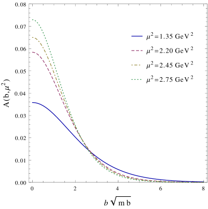
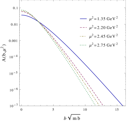
In our form factor model, this corresponds to
| (17) |
The shapes of the overlap function for those values of are shown in Fig 2. The value from the previous tune of Herwig++, ue-ee-4-cteq6l1, with , is shown for comparison. It is clearly well outside the range given by the measurements.
4 Tuning to the underlying event data
In this section we address the question of whether the MPI model in Herwig++ is consistent with the and underlying event (UE) data. To that end we need to check whether it is possible to find values of the free parameters of the MPI model that allow a good description of the experimental data. As described in Sect. 2, the MPI model in Herwig++ has five parameters that we consider freely tunable: , , , and . Because we are dealing with a large number () of tunable parameters, a simple tuning strategy of subdividing the -dimensional parameter space into a grid and for each of the parameter points on this grid running Herwig++ and calculating the total against the experimental data, is ineffective. A comprehensive scan of 5 parameters, with 10 divisions in each parameter, would require too much CPU time.
Instead, we use the parametrization-based tune method provided by the Professor package Buckley:2009bj , which is much more efficient for our case. The starting point for this tuning procedure is the selection of a range for each of the tuning parameters . Event samples are generated for random points in this -dimensional hypercube in parameter space. The number of points sampled is chosen, depending on the number of input parameters, to ensure good control of the final tune. Each generated event is directly handed over to the Rivet package Buckley:2010ar , which implements the experimental analyses. Thus the results for each observable are calculated at each set of parameter values. Professor parametrizes each bin of each histogram as a function of the input parameters. It is then able to find the set of parameters that fits the selected observables best. As a user, one simply has to choose the set of observables that one wishes to tune to and, optionally, their relative weights in the fit.
4.1 Observables
On top of the data mentioned above we examine a set of standard UE observables at different collider energies whose description is sensitive to the MPI model parameters. The standard UE measurements are made relative to a leading object (the hardest charged track or jet). Then, the transverse plane is subdivided in azimuthal angle relative to this leading object at . The region around the leading object, , is called the “towards” region. The opposite region, where we usually find a recoiling hard object, , is called the “away” region, while the remaining region, transverse to the leading object and its recoil, called the “transverse” region, is expected to be the most sensitive to MPI activity. The UE experimental data used for the tune should be measured at a wide range of collider energies in similar phase-space regions and under not too different trigger conditions. These conditions are met by two UE observables:
-
•
The mean number of stable charged particles per unit of -: , in the tranverse region;
-
•
The mean scalar sum of stable particles: , in the tranverse region.
Both are measured as a function of (with ) by ATLAS at \unit900 and \unit7 (with 333For data collected at \unit7 we also used observables with .)Aad:2010fh and by CDF at \unit300, \unit900 and \unit1960 (with )CDFUEscan . In both ATLAS and CDF UE analyses, denotes the transverse momentum of the hardest track444CMS have also made measurements of the underlying event, but using track-based jetsChatrchyan:2011id . We confine ourselves to ATLAS’s hardest-track analysis here, since this matches most closely CDF’s energy scan analyses, giving us the longest lever arm in energy for a single analysis type..
Between all of the above data, we have a total of 132 histogram bins for each of and at various collider energies and values to fit the model parameters to, as well as the value of . By default, Professor would treat each of these 265 pieces of data equally, and would not pay any more attention to reproducing the value of than it would to any individual histogram bin. On the contrary, we would like to treat each type of data, , and , on an equal footing. We therefore use the option provided by Professor 555We also modified Professor to use the exact analytical formula for , Eq. (10), rather than the value calculated by the Monte Carlo algorithm, which has (small) numerical errors. to apply different weights to different observables (see Eq. (18)). We give each of the histogram bins unit weight, while we give a weight of 132 666We show the weight-dependence of our result in Appendix A.1, where it can be seen that any weight value above about 100 would give similar results, within 1 of the input value..
As we discussed in the introduction, MPI model parameters should be used together with the pdf set with which they have been tuned. Thus, in the Herwig convention, the name of the tune contains the name of the pdf set. We have used leading order version 6.1 pdfs from the CTEQ collaboration Stump:2003yu and therefore, to fit the naming conventions of Herwig, call our final tune “ue-ee-5-cteq6l1”777We have also produced a corresponding set using the MSTW LO* pdfs Martin:2009iq . Although the tuned parameters differ somewhat, the results for and UE observables do not differ significantly, so we do not show the results here.. In order to study how fitting the value of influences the result of the tune we also performed a tune without taking into account the data. We will refer to this tune as “No in fit”.
4.2 Results
We begin by showing the weighted value calculated by Professor:
| (18) |
where is the weight for bin of observable , is a function of the tuning parameters , which parametrizes the Monte Carlo results, is the reference (experimental) value for bin and the error is the total uncertainty888In practice we attempt to generate sufficient events at each sampled parameter point that the statistical Monte Carlo error is much smaller than the reference error for all bins. for bin . Recall that we use except for , which has .
In the left panel of Fig. 3, we plot the value as a function of and fitting only to the UE data, i.e. the “No in fit” fit.
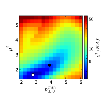
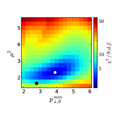
For each parameter pair, we show the minimum that can be found in the corresponding subspace of the other parameters, , and . We see that the function forms a long thin valley, with a strong correlation between and . This reflects the fact that a smaller hadron radius means more multiple scattering, which can be compensated to give a similar amount of underlying-event activity by having fewer perturbative MPIs, i.e. a larger value of . The best fit value is , , but one can obtain good fits up to at least , provided is adjusted accordingly.
In the right panel of Fig. 3, we plot the equivalent results including the measurement with a weight of 132, i.e. the ue-ee-5-cteq6l1 fit. As would be expected, the inclusion of the data helps to break the degeneracy between and , favouring the range that reproduces the value. On the other hand the description of the UE data is not significantly worsened, as can be seen from the fact that the best fit with lies ‘on the valley floor’ of the fit without .
It is worth making several comments here on the values of obtained in these plots. Firstly, Professor’s definition of “” includes the weight factors and, hence, is 1.5 times larger in the plot on the right than the plot on the left. Secondly, while the experimental data points have moderate point-to-point correlations, the theoretical predictions are strongly correlated: the shapes of the curves are reasonably stable predictions and it is mainly their normalization that varies in response to the variation of parameters. Our aim is to get a reasonable description of that normalization across a wide range of collider energies. We therefore can definitely not interpret in a strict statistical sense. Finally, the value plotted is Professor’s prediction of the at a given point, based on a parametrization of the Monte Carlo results, which have statistical errors. The values themselves therefore have errors. For example, in Appendix A.2 we compare a Monte Carlo run at the best fit point (with ) with the Professor prediction for it (with ). We consider anywhere in the valley floor with up to about 5 in the left-hand plot to be a reasonable description of the underlying event data.
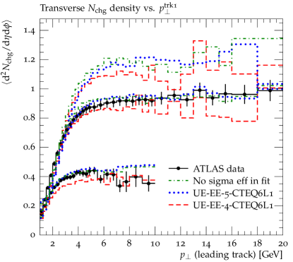
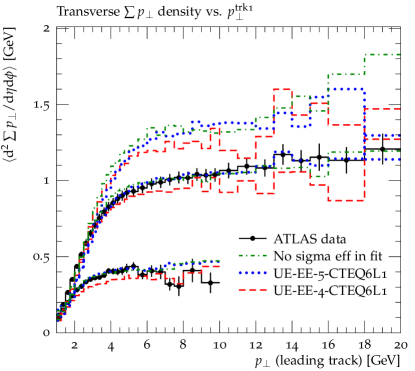
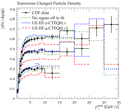
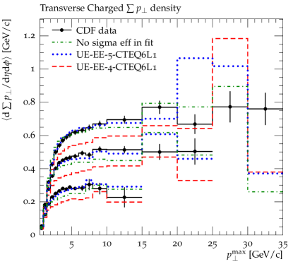
In Figs. 4 and 5, we show the description of the UE data from ATLAS and CDF respectively. We see that the “No in fit” and ue-ee-5-cteq6l1 fits do indeed describe the data equally well, and significantly better than the previous ue-ee-4-cteq6l1 fit, which is the default tune of Herwig++ 2.6 Arnold:2012fq . The values of the tuned parameters are given in Table 1.
Figure 4 also shows the prediction for results at 14 where, again, the results of the “No in fit” and ue-ee-5-cteq6l1 fits are very similar, showing that requiring the fits to describe has not biased the UE results significantly.
| ue-ee-4-cteq6l1 | “No in fit” | ue-ee-5-cteq6l1 | |
|---|---|---|---|
| 1.35 | 1.65 | 2.30 | |
| 0.75 | 0.22 | 0.80 | |
| 0.61 | 0.60 | 0.49 | |
| 2.81 | 2.80 | 3.91 | |
| 0.24 | 0.29 | 0.33 |
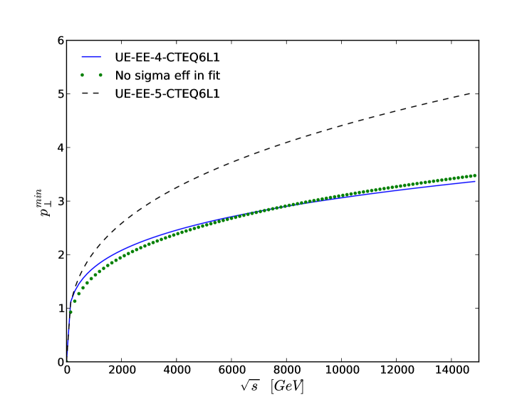
Finally, in Fig. 6, we show the dependence of on the collision energy. The “No in fit” fit is very similar to the previous default, whereas we have seen that their UE predictions are quite different, owing to the different values of the other parameters. On the other hand, the “No in fit” fit and our new best fit, ue-ee-5-cteq6l1, are quite different, but the correlation with the other fit parameters means that their UE predictions are very similar. This clearly shows the importance of the simultaneous fit of all parameters and the danger of ascribing too much physical significance to the value of one parameter in isolation of the others.
5 Conclusions
We have discussed the experimental measurements of from double-parton scattering. We concluded that, over the energy range from the Tevatron to the LHC, there is no evidence that is energy dependent. The best value of at present comes from a combination of the CDF and D0 measurements.
We have also studied fits of our MPI model parameters to underlying event data from CDF and ATLAS over the collision energy range from 300 to 7 . It is commonly stated that there is a conflict between such fits and the value of . Indeed, we have seen that our best fit to the UE data yields , almost 5 from its measured value.
However, we have also seen that by including in the fit, with the same weight as the sum of each of the multiplicity and sum data, we are able to obtain a set of parameters that yields , less than 1 from its measured value, without significantly worsening the description of the underlying event data. The extrapolation to 14 is likewise unaffected. It is worth noting that other model parameters are significantly different between the two tunes, emphasising the importance of simultaneous tuning.
We conclude that it is possible to describe the double-parton scattering cross section and underlying event final states with a common set of parameters in the Herwig MPI model. The parameter set ue-ee-5-cteq6l1 will be the default set with the next Herwig++ release.
Acknowledgements.
We are grateful to the Cloud Computing for Science and Economy project (CC1) at IFJ PAN (POIG 02.03.03-00-033/09-04) in Cracow whose resources were used to carry out all the numerical calculations for this project. Thanks also to Mariusz Witek and Miłosz Zdybał for their help with CC1 and Hendrik Hoeth for his help with Professor. This work was funded in part by the Lancaster-Manchester-Sheffield Consortium for Fundamental Physics under STFC grant ST/J000418/1 and in part by the MCnetITN FP7 Marie Curie Initial Training Network PITN-GA-2012-315877.Appendix A Tuning details
In this appendix we briefly show a couple of more technical features related to our fits.
A.1 Dependence on the weights
We argued earlier that an appropriate weight to use for in the Professor fits is 132, giving it the same weight as all the multiplicity or sum data. We have also studied the dependence of the tune on the weight applied.
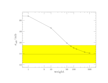
In Fig. 7 we show the best fit value of as a function of the weight applied. We see that the weight needs to be at least about 70 to bring the value of within 1 of its measured value, and that increasing it significantly beyond about 250 has almost no further effect. We conclude that 132 is a sensible value for the weight, but that the results are not critically dependent on its precise value, within a factor of two.
The fact that the UE results are so similar between the “No in fit” fit, which effectively has weight, and the ue-ee-5-cteq6l1 fit, with weight, is a confirmation that they do not depend significantly on the weight applied.
A.2 Stability of Professor predictions
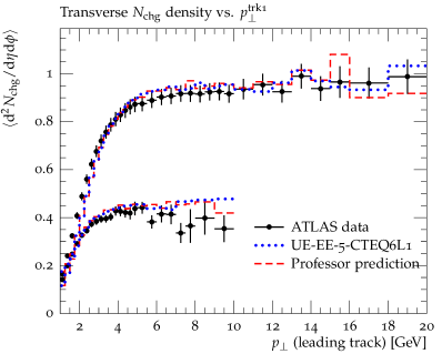
All of our tuning has been performed using Professor’s parametrization of Herwig++’s results as a function of its parameters. As a cross-check that this parametrization is reliable, we show in Figs. 8 and 9 the comparison of Monte Carlo runs with the ue-ee-5-cteq6l1 parameter set with Professor’s prediction of them. They can be seen to agree very well.
We also mention that we only fitted to the regions of the plots where the experimental and Monte Carlo statistical errors are small emough that fluctuations are not significant. Specifically, we use the data with at 300 , at 900 , at 1960 and at 7 . By eye, one can see that the results are reliable beyond the region to which they are fit.
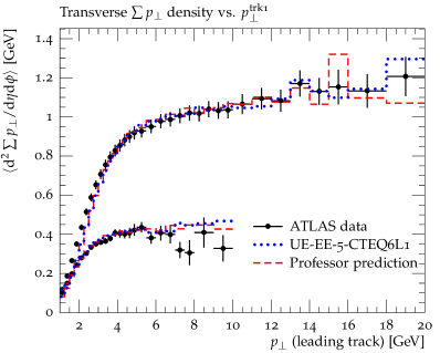
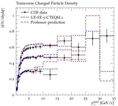
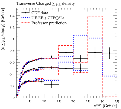
References
- (1) T. Sjöstrand and M. van Zijl, A Multiple Interaction Model for the Event Structure in Hadron Collisions, Phys.Rev. D36 (1987) 2019.
- (2) G. Marchesini and B. R. Webber, Associated transverse energy in hadronic jet production, Phys.Rev. D38 (1988) 3419.
- (3) AFS Collaboration, T. Åkesson et al., Double parton scattering in p p collisions at s**(1/2) = 63-GeV, Z.Phys. C34 (1987) 163.
- (4) UA2 Collaboration, J. Alitti et al., A Study of multi - jet events at the CERN anti-p p collider and a search for double parton scattering, Phys.Lett. B268 (1991) 145–154.
- (5) CDF Collaboration, F. Abe et al., Study of four jet events and evidence for double parton interactions in collisions at TeV, Phys.Rev. D47 (1993) 4857–4871.
- (6) CDF Collaboration, F. Abe et al., Double parton scattering in collisions at TeV, Phys.Rev. D56 (1997) 3811–3832.
- (7) D0 Collaboration, V. M. Abazov et al., Double parton interactions in photon+3 jet events in bar collisions TeV, Phys.Rev. D81 (2010) 052012, [arXiv:0912.5104].
- (8) LHCb Collaboration, R. Aaij et al., Observation of pair production in collisions at , Phys.Lett. B707 (2012) 52–59, [arXiv:1109.0963].
- (9) LHCb Collaboration, R. Aaij et al., Observation of double charm production involving open charm in pp collisions at =7 TeV, JHEP 1206 (2012) 141, [arXiv:1205.0975].
- (10) ATLAS Collaboration, G. Aad et al., Measurement of hard double-parton interactions in jet events at TeV with the ATLAS detector, New J.Phys. 15 (2013) 033038, [arXiv:1301.6872].
- (11) S. Gieseke, C. A. Röhr, and A. Siódmok, Multiple Partonic Interaction Developments in Herwig++, arXiv:1110.2675.
- (12) S. Gieseke, D. Grellscheid, K. Hamilton, A. Papaefstathiou, S. Plätzer, et al., Herwig++ 2.5 Release Note, arXiv:1102.1672.
- (13) S. Gieseke, C. Röhr, and A. Siódmok, Colour reconnections in Herwig++, Eur.Phys.J. C72 (2012) 2225, [arXiv:1206.0041].
- (14) K. Arnold, L. d’Errico, S. Gieseke, D. Grellscheid, K. Hamilton, et al., Herwig++ 2.6 Release Note, arXiv:1205.4902.
- (15) R. Corke and T. Sjöstrand, Interleaved Parton Showers and Tuning Prospects, JHEP 1103 (2011) 032, [arXiv:1011.1759].
- (16) T. Sjöstrand and P. Z. Skands. Private communication.
- (17) P. Z. Skands, The Perugia Tunes, arXiv:0905.3418.
- (18) P. Bartolini. Private communication.
- (19) M. Strikman, Transverse Nucleon Structure and Multiparton Interactions, Acta Phys.Polon. B42 (2011) 2607–2630, [arXiv:1112.3834].
- (20) L. Frankfurt, M. Strikman, and C. Weiss, Transverse nucleon structure and diagnostics of hard parton-parton processes at LHC, Phys.Rev. D83 (2011) 054012, [arXiv:1009.2559].
- (21) R. Corke and T. Sjöstrand, Multiparton Interactions with an x-dependent Proton Size, JHEP 1105 (2011) 009, [arXiv:1101.5953].
- (22) B. Blok, Y. Dokshitzer, L. Frankfurt, and M. Strikman, Perturbative QCD correlations in multi-parton collisions, arXiv:1306.3763.
- (23) H. Abramowicz, P. Bartalini, M. Bähr, N. Cartiglia, E. Dobson, et al., Summary of the Workshop on Multi-Parton Interactions (MPI@LHC 2012), arXiv:1306.5413.
- (24) J. M. Butterworth, J. R. Forshaw, and M. H. Seymour, Multiparton interactions in photoproduction at HERA, Z.Phys. C72 (1996) 637–646, [hep-ph/9601371].
- (25) I. Borozan and M. H. Seymour, An Eikonal model for multiparticle production in hadron hadron interactions, JHEP 0209 (2002) 015, [hep-ph/0207283].
- (26) M. Bähr, S. Gieseke, and M. H. Seymour, Simulation of multiple partonic interactions in Herwig++, JHEP 0807 (2008) 076, [arXiv:0803.3633].
- (27) M. Bähr, S. Gieseke, M. A. Gigg, D. Grellscheid, K. Hamilton, et al., Herwig++ Physics and Manual, Eur.Phys.J. C58 (2008) 639–707, [arXiv:0803.0883].
- (28) D. Treleani, Double parton scattering, diffraction and effective cross section, Phys.Rev. D76 (2007) 076006, [arXiv:0708.2603].
- (29) M. Bähr, M. Myska, M. H. Seymour, and A. Siódmok, Extracting sigma effective from the CDF gamma+3jets measurement, JHEP 1303 (2013) 129, [arXiv:1302.4325].
- (30) R. Maciula and A. Szczurek, Production of in double-parton scattering within -factorization approach – meson-meson correlations, arXiv:1301.4469.
- (31) A. V. Berezhnoy, A. K. Likhoded, A. V. Luchinsky, and A. A. Novoselov, Double production at LHCb, Phys.Rev. D86 (2012) 034017, [arXiv:1204.1058].
- (32) A. Buckley, H. Hoeth, H. Lacker, H. Schulz, and J. E. von Seggern, Systematic event generator tuning for the LHC, Eur. Phys. J. C65 (2010) 331–357, [arXiv:0907.2973].
- (33) A. Buckley, J. M. Butterworth, L. Lönnblad, H. Hoeth, J. Monk, et al., Rivet user manual, arXiv:1003.0694.
- (34) ATLAS Collaboration, G. Aad et al., Measurement of underlying event characteristics using charged particles in pp collisions at and 7 TeV with the ATLAS detector, Phys.Rev. D83 (2011) 112001, [arXiv:1012.0791].
- (35) CDF Collaboration, R. Field, C. Group, and D. Wilson, The Energy Dependence of the Underlying Event in Hadronic Collisions, . talk presented by R. Field at the 36th International Conference on High Energy Physics (ICHEP 2012), Melbourne, Australia, July 5, 2012; and CDF physics note CDF/ANAL/CDF/CDFR/10874, unpublished.
- (36) CMS Collaboration Collaboration, S. Chatrchyan et al., Measurement of the Underlying Event Activity at the LHC with TeV and Comparison with TeV, JHEP 1109 (2011) 109, [arXiv:1107.0330].
- (37) D. Stump, J. Huston, J. Pumplin, W.-K. Tung, H. L. Lai, et al., Inclusive jet production, parton distributions, and the search for new physics, JHEP 0310 (2003) 046, [hep-ph/0303013].
- (38) A. D. Martin, W. J. Stirling, R. S. Thorne, and G. Watt, Parton distributions for the LHC, Eur.Phys.J. C63 (2009) 189–285, [arXiv:0901.0002].