Efimov-driven phase transitions of the unitary Bose gas
Supplementary information

1 Model hamiltonian and unitary limit

The pair interaction in the model hamiltonian may be viewed as the zero-range limit of the square-well interaction potential shown in Supplementary Fig. 1, whose range $r_{0}$ and depth $V_{0}$ are simultaneously taken to $0$ and $\infty$ so that the scattering length $a=r_{0}\left[1-\tan(r_{0}\sqrt{mV_{0}/\hbar^{2}})/(r_{0}\sqrt{mV_{0}/\hbar^{2}})\right]$ remains constant. At zero range, the pair interaction only affects $s$-waves by the so-called Bethe-Peierls limit condition when the separation $r$ between two particles goes to zero.

Unitarity corresponds to the pair interaction having a bound dimer of zero energy and infinite extension, a limit in which the $k$-vector of the particle is much smaller than $1/r_{0}$, and the scattering cross-section $\sigma$ saturates the unitary limit $\sigma<8\pi/k^{2}$. This follows from the unitarity of the scattering operator.

Supplementary Figure 1: Illustration of square pair interaction potentials in the unbound region $R_{0}/a\sim-1$ (left), in the unitary region $R_{0}/a=0$ (centre), and in the bound pair + particle region $R_{0}/a\sim 1$ (right). The zero-range potential is fixed-$a$ limit of these potentials when $V_{0}\to\infty$ and $r_{0}\to 0$. The (possible) pair bound state correspond to cyan levels.

While the two-particle properties are universal, the three-boson trimer ground state at unitarity generally depends on the details of the pair interaction. Excited trimers form a geometric sequence of asymptotically universal Efimov trimers with a fixed energetic ratio $E_{n}/E_{n+1}\underset{n\to\infty}{\rightarrow}515.03$, where $E_{n}$ is the energy of the $n$-th excited trimer. For the zero-range pair interaction and the three-body hard core, the ground-state trimer is almost identical to universal Efimov trimers[1].

2 Dedicated Path-Integral Monte Carlo algorithm

In our Path-Integral Monte Carlo algorithm, statistical weights due to the two-body and three-body interactions in the model hamiltonian are computed as follows:

• the zero-range interaction is implemented through the pair-product approximation for the density matrix, that estimates the statistical weight of a configuration from the isolated two-body wavefunction of nearby particles. For the zero-range interaction, only $s$-waves differ from the isolated system of two non-interacting bosons. The pair-product approximation is valid when the imaginary time discretization step $\Delta\tau$ is small enough.

• The hyperradial cutoff $V_{3}$ is enforced by rejecting the configurations where the hyperradius is smaller than a threshold $R_{0}$, an approximation also valid if $\Delta\tau$ is small enough. In practice, for the values of $\Delta\tau$ retained in our simulations, we need to take in account a finite $\Delta\tau$ shift of the input value of $R_{0}$, which we compute from a fit of the three-particle hyperradial probability distribution to its analytically-known value[1],

  $$p(R)\propto RK^{2}_{is_{0}}\left(\sqrt{2}\kappa R\right),$$

  where $K_{is_{0}}$ a Bessel function of imaginary index $is_{0}\approx 1.00624i$, and $\kappa^{2}=mE_{t}/\hbar^{2}\propto R_{0}^{-2}$.

These weights set the probability of acceptance of the following four types of Markov-chain moves, following a Metropolis-Hastings procedure.

1. Rebuild a single-particle path on a fraction of the total imaginary time,

2. Move a whole permutation cycle,

3. Exchange two strands of paths on a fraction of the total imaginary time,

4. Perform a compression-dilation move on one imaginary time slice (see Supplementary Fig. 2).

Supplementary Figure 2: Compression-dilation move (move (4)). At one imaginary time slice, the new proposed positions for two particles (blue paths) are either more distant or closer by a factor $1+h$ while the centre of mass (white circles) and positions at other time slices are kept in place.

Updates (1-3) are commonly used in Path-Integral Monte Carlo simulations[2, 3, 4]. The compression-dilation move (4) specifically addresses the divergence of the pair-distance distribution function (see Fig.1d): Even when it rebuilds a path on one single imaginary time slice, the update (1) is linear: if two particles are separated by a distance $r$, it will typically propose a new configuration with a separation $r+\Delta$. The weight of the proposed configuration $w(r+\Delta)$ is quite different from the weight of the original configuration $w(r)$ when $r\to 0$, which results in a very low acceptance rate. The update (4) proposes a configuration $r(1+h)$, whose weight $w(r)+hrw^{\prime}(r)$ is close to $w(r)$: Because $w(r)$ diverges as $1/r^{2}$, $rw^{\prime}(r)$ is of the same order as $w(r)$, which generates much higher acceptance rates.

3 Cocyclicity condition and graphic representation in Fig.1

In our simulations of unitary bosons, the system is contained in a harmonic trap, which regulates the available configuration space. To reduce entropic effects for the three-body calculations in Fig.1, we regulate the volume by imposing that they lie on a single permutation cycle: In Fig.1a-c, at imaginary time $\beta$, the blue, red and green bosons are respectively exchanged with the red, green and blue bosons. This condition does not modify the properties of the fundamental trimers as other permutations could be sampled at no cost at points of close encounters, some of which are highlighted in Fig.1b.

In Fig.1a-c, four-dimensional co-cyclic path-integral configurations are represented in a three-dimensional plot. As the motion of the centre of mass is decoupled from the effects of the interactions, its position is set to zero at all $\tau$. The three spatial dimensions are then reduced to two dimensions by rotating the triangle formed by the three particles at each imaginary time to the same plane in a way that does not favour any of the three spatial dimensions, but that conserves the permutation cycle structure. This transformation conserves the pair distances.

4 High-temperature equation of state

The local density approximation consists in assuming that, at each point $\mathbf{x}=(x,y,z)$ of the trap, with $|\mathbf{x}|=r$, the Bose gas is in equilibrium at a chemical potential $\mu=\mu_{0}-\omega^{2}r^{2}/2$, where $\mu_{0}$ is the chemical potential in the trap centre. Within this approximation, thermodynamical identities allow one to relate the doubly-integrated density profile $\bar{n}(x)$, and the grand-canonical pressure[5]:

$$P(\mu(x))=\frac{\omega^{2}}{2\pi}\bar{n}(x),$$ (1)

where $\mu(x)=\mu_{0}-\omega^{2}x^{2}/2$. The chemical potential $\mu_{0}$ at the centre of the trap can be obtained from a fit in the outer region of the trap where $P(\mu)$ is the pressure of a classical ideal gas.

The doubly-integrated density profile is obtained by ensemble averaging, and the numerical equation of state $P(\mu)$ is compared to the expansion of the pressure in powers of the fugacity $e^{\beta\mu}$ (see Fig.3),

$$P=\frac{k_{B}T}{\lambda^{3}}\sum_{l\geq 1}b_{l}e^{l\beta\mu}.$$ (2)

The $l$-th cluster integral $b_{l}$ corresponds to the $l$-body effects that cannot be reduced to smaller non-interacting groups of interacting particles[6]. The classical ideal gas corresponds to $b_{1}=1$, and higher coefficients both describe both energetic and quantum-statistical correlations. The $l$-th cluster integrals are related to the virial coefficients $\{a_{l^{\prime}}\}_{l^{\prime}\leq l}$[6] as

$$\begin{cases}b_{1}=a_{1}=1,\\ b_{2}=-a_{2},\\ b_{3}=-\frac{1}{2}a_{3}+2a_{2}^{2}.\end{cases}$$ (3)

At unitarity, an analytical expression of the coefficients $b_{2}$ and $b_{3}$ was obtained recently[7], $b_{2}=9/(4\sqrt{2})\approx 1.59$, and

$$\frac{b_{3}}{3\sqrt{3}}=C+\sum_{q\geq 0}\left(e^{-\beta\epsilon_{q}}-1\right)+\frac{|s_{0}|}{\pi}\left\{\frac{1}{2}\ln\left(e^{\gamma}\beta E_{t}\right)-\sum_{p\geq 1}e^{-p\pi|s_{0}|}\Re\left[\Gamma(-ip|s_{0}|)(\beta E_{t})^{ip|s_{0}|}\right]\right\},$$ (4)

where $C=0.648$ and $|s_{0}|=1.00624$ are two constants, $\gamma=0.577$ is the Euler constant, $\epsilon_{q}=-E_{t}e^{-2\pi q/|s_{0}|}$ represents the energy levels of the three-body bound states, and $-E_{t}$ is the energy of the fundamental Efimov trimer, which is related to the average squared hyperradius in the fundamental state[1]:

$$E_{t}=\frac{2(1+s_{0}^{2})}{3\left\langle R^{2}\right\rangle},$$ (5)

an expression that may be used to obtain $E_{t}\approx 4.27e^{-3}\hbar^{2}/(mR_{0}^{2})$ by numerically integrating Eq. • ‣ 2.

In the temperature range of our simulations, it is sufficient to perform the sums in Eq. 4 up to $q=1$.

5 Monitoring the phase transition

When the densities of the gas and the superfluid Efimov liquid approach each other, observing directly the two-dimensional histogram of pair distances and centre-of-mass positions does not allow to distinguish between a weakly first-order phase transition and a cross-over (see Supplementary Fig. 3).

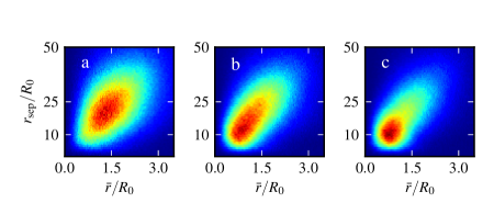
Supplementary Figure 3: Two-dimensional histogram of pair distances $r_{\text{sep}}$ and centre-of-mass positions $\bar{r}$ for $R_{0}=1.3$, at $k_{B}T/\hbar\omega=4.3.$ (a), $k_{B}T/\hbar\omega=4.2$ (b), and $k_{B}T/\hbar\omega=4.0$. The sole observation of this histogram does not allow here to state that the system is undergoing a phase transition as the densities of both phases are too close.

In this regime, we monitor the normal-gas-to-superfluid-liquid phase transition more accurately by following the evolution of the first peak of the pair correlation function (obtained by ensemble averaging) with temperature (see Supplementary Fig. 4).

Supplementary Figure 4: Evolution of the position of the first peak of the pair correlation function for several values of $R_{0}$. For $R_{0}/a_{\omega}=0.07$, the large step indicates the first order phase transition (this corresponds to Fig.3a-c); at $R_{0}/a_{\omega}=0.13$, the step persists but is considerably smaller, a sign that the system also undergoes a first order phase transition. At $R_{0}/a_{\omega}=0.23$, there is no sign of a first order phase transition.

For each value of $R_{0}$, simulations in the trap are run at a discrete set of inverse temperature $\beta$. In Fig.4a, the error bars in the normal-gas-to-superfluid-liquid transition line show the interval between the last temperature at which there is no liquid droplet, and the first temperature at which there is one. The errors for the conventional superfluid transition are computed in the same way, with the criterion that the gas is superfluid if particles lie in a permutation cycle of length at least ten with a probability higher than $0.05$.

6 Approximate semi-analytical phase diagram

When the free energy $F$ of a homogeneous physical system is not a convex function of its volume $V$, it becomes more favourable to split the system into two phases than to keep the system homogeneous, a situation from which first order phase transitions originate (see Supplementary Fig. 5), and that yields the equality of the pressures and of the chemical potentials of both phases at coexistence in absence of interface energy[8].

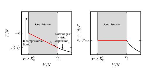
Supplementary Figure 5: Sketch of the behaviour of the free energy and the pressure of unitary bosons through the transition in our incompressible fluid model.

In the system of unitary bosons, the virial expansion is an excellent approximation for the normal gas phase far from the superfluid transition. Although it becomes irrelevant in the superfluid gas, its analytic continuation conveys important qualitative features, because of the continuous nature of the normal-gas-to-superfluid-gas phase transition, and is therefore a suitable poor man’s approximation to the behaviour of the superfluid gas.

The simplest theoretical model for the superfluid liquid is that of an incompressible liquid of specific volume $v_{l}$ and negligible entropic contribution to the free energy. The incompressibility approximation is acceptable for unitary bosons as the first peak of the pair correlation function seems to scale only with $R_{0}$ (see Fig.2); simulations at high $R_{0}$ yield $v_{l}\approx(6R_{0})^{3}$. The negligibility of the entropic contribution to the free energy is ensured for non-pathological systems at low temperature. As results of Ref.[9] may be extrapolated to obtain an energy per particle $-\epsilon=-10.1E_{t}$ in the liquid phase (see Supplementary Fig. 6), in this approximation, the free energy is $F_{l}=-N\epsilon$.

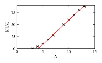
Supplementary Figure 6: Energy of clusters of unitary bosons at zero temperature (black crosses) as a function of the number $N$ of bosons in the cluster, computed by J. von Stecher in Ref.[9], in units of the fundamental Efimov trimer energy $E_{t}$. A linear regression (solid red line) gives $|E|/N=10.1E_{t}$ for large $N$ values. For the phase diagram of $100$ bosons in a harmonic trap (Fig.4a), the value of $|E|/N$ is empirically adjusted to $8E_{t}$ to account for the small number of bosons in the liquid droplet.

In practice, we draw the transition line into the superfluid liquid by finding the smallest chemical potential at which the pressures of the incompressible liquid and of the gas phase (approximated by the virial expansion) coincide:

$$\frac{\mu-\epsilon}{v_{l}}=\frac{k_{B}T}{\lambda^{3}}\left(e^{\beta\mu}+b_{2}e^{2\beta\mu}+b_{3}e^{3\beta\mu}\right).$$ (6)

As $1/v=\partial_{\mu}P$, the crossing to the regime where this equation has no solution corresponds to the critical point, where both densities are equal.

To draw the coexistence line for the trap centre with $N=100$ particles, the chemical potential $\mu_{0}$ at the centre of the trap is found from integrating the density throughout the trap:

$$\frac{4\pi}{\lambda^{3}}\int_{0}^{\infty}r^{2}dr\left(e^{\beta\mu(r)}+2b_{2}e^{2\beta\mu(r)}+3b_{3}e^{3\beta\mu(r)}\right)=N,$$ (7)

where $\mu(r)=\mu_{0}-\omega^{2}r^{2}/2$.

References

- [1] Braaten, E. & Hammer, H.-W. Universality in few-body systems with large scattering length. Phys. Rep. 428, 259–390 (2006).
- [2] Pollock, E. L. & Ceperley, D. M. Simulation of quantum many-body systems by path-integral methods. Phys. Rev. B 30, 2555–2568 (1984).
- [3] Krauth, W. Quantum Monte Carlo calculations for a large number of bosons in a harmonic trap. Phys. Rev. Lett. 77, 3695–3699 (1996).
- [4] Krauth, W. Statistical Mechanics: Algorithms and Computations (Oxford University Press, Oxford, Great Britain, 2006).
- [5] Ho, T.-L. & Zhou, Q. Obtaining the phase diagram and thermodynamic quantities of bulk systems from the densities of trapped gases. Nature Phys. 6, 131–134 (2010).
- [6] Huang, K. Statistical mechanics (Wiley, New York, 1987), 2nd edn.
- [7] Castin, Y. & Werner, F. Le troisième coefficient du viriel du gaz de bose unitaire. Canad. J. Phys. 91, 382–389 (2013). arxiv:1212/5512 (English version).
- [8] Landau, L. D. & Lifshitz, L. M. Statistical physics. No. 5 in Course of theoretical physics (Butterworth-Heinemann, 1980), 3rd edn.
- [9] von Stecher, J. Weakly bound cluster states of Efimov character. J. Phys. B 43, 101002 (2010).