Phase structure of two-dimensional QED at zero temperature with flavor-dependent chemical potentials and the role of multidimensional theta functions

Abstract

We consider QED on a two-dimensional Euclidean torus with $f$ flavors of massless fermions and flavor-dependent chemical potentials. The dependence of the partition function on the chemical potentials is reduced to a $(2f-2)$-dimensional theta function. At zero temperature, the system can exist in an infinite number of phases characterized by certain values of traceless particle numbers and separated by first-order phase transitions. Furthermore, there exist many points in the $(f-1)$-dimensional space of traceless chemical potentials where two or three phases can coexist for $f=3$ and two, three, four or six phases can coexist for $f=4$. We conjecture that the maximal number of coexisting phases grows exponentially with increasing $f$.

I Introduction and Summary

QED in two dimensions is a useful toy model to gain an understanding of the theory at finite temperature and chemical potential Sachs:1993zx ; Sachs:1995dm ; Sachs:1991en . In particular, the physics at zero temperature is interesting since one can study a system that can exist in several phases. The theory at zero temperature is governed by two degrees of freedom often referred to as the toron variables in a Hodge decomposition of the U(1) gauge field on a $l\times\beta$ torus where $l$ is the circumference of the spatial circle and $\beta$ is the inverse temperature. Integrating over the toron fields projects on to a state with net zero charge Gross:1980br and therefore there is no dependence on a flavor-independent chemical potential Narayanan:2012du . The dependence on the isospin chemical potential for the two flavor case was studied in Narayanan:2012qf and we extend this result to the case of $f$ flavors in this paper. After integrating out the toron variables, the dependence on the $(f-1)$ traceless chemical potential variables and the dimensionless temperature $\tau=\frac{l}{\beta}$ can be written in the form of a $(2f-2)$-dimensional theta function (see multitheta for an overview on multidimensional theta functions). The $(2f-2)$ dimensional theta function has a non-trivial Riemann matrix and this is a consequence of the same gauge field (toron variables, in particular) that couples to all flavors. The resulting phase structure is quite intricate since it involves minimization of a quasi-periodic function over a set of integers. We will explicitly show:

1. Three flavors: The two-dimensional plane defined by the two traceless chemical potentials is filled by hexagonal cells (c.f. Fig. 4 in this paper) with the system having a specific value of the two traceless particle numbers in each cell and neighboring cells being separated by first-order phase transitions at zero temperature. The vertices of the hexagon are shared by three cells and therefore two or three different phases can coexist at zero temperature.

2. Four flavors: The three-dimensional space defined by the three traceless chemical potentials is filled by two types of cells (c.f. Fig. 8 in this paper). One of them can be viewed as a cube with the edges cut off. We then stack many of these cells such that they join at the square faces. The remaining space is filled by the second type of cell. All edges of either one of the cells are shared by three cells but we have two types of vertices – one type shared by four cells and another shared by six cells. At zero temperature, each cell can be identified by a unique value for the three different traceless particle numbers and neighboring cells are separated by first-order phase transitions. Therefore, two, three, four or six phases can coexist at zero temperature.

One can use the multidimensional theta function to study the phase structure when $f>4$ but visualization of the cell structure becomes difficult. Nevertheless, it is possible to provide examples of the coexistence of many phases. We conjecture that the maximal number of coexisting phases is given by $f\choose{\lfloor f/2\rfloor}$, increasing exponentially for large $f$.

The organization of the paper is as follows. We derive the dependence of the partition function on the $(f-1)$ traceless chemical potentials and the dimensionless temperature $\tau$ in section II. We briefly show the connection to the two flavor case discussed in Narayanan:2012qf and focus in detail on the three and four flavor cases in section III. We then conclude the paper with a discussion of some examples when $f>4$.

II The partition function

Consider $f$-flavored massless QED on a finite torus with spatial length $l$ and dimensionless temperature $\tau$. All flavors have the same gauge coupling $\frac{e}{l}$ where $e$ is dimensionless. Let

$$\mbox{\boldmath$\mu$}^{t}=\begin{pmatrix}\mu_{1}&\mu_{2}&\cdots&\mu_{f}\cr\end{pmatrix}$$ (1)

be the flavor-dependent chemical potential vector. The partition function is Sachs:1991en ; Narayanan:2012qf

$$Z(\mbox{\boldmath$\mu$},\tau,e)=Z_{b}(\tau,e)Z_{t}(\mbox{\boldmath$\mu$},\tau),$$ (2)

where the bosonic part is given by

$$Z_{b}(\tau,e)=\frac{1}{\eta^{2f}(i\tau)}\sideset{}{{}^{\prime}}{\prod}_{k_{1},k_{2}=-\infty}^{\infty}\frac{1}{\sqrt{\left(k_{2}^{2}+\frac{1}{\tau^{2}}k_{1}^{2}\right)\left(k_{2}^{2}+\frac{1}{\tau^{2}}\left[k_{1}^{2}+\frac{fe^{2}}{4\pi^{3}}\right]\right)}}$$ (3)

(with $k_{1}=k_{2}=0$ excluded from the product and $\eta(i\tau)$ being the Dedekind eta function) and the toronic part reads

$$Z_{t}(\mbox{\boldmath$\mu$},\tau) =\int_{-\frac{1}{2}}^{\frac{1}{2}}dh_{2}\int_{-\frac{1}{2}}^{\frac{1}{2}}dh_{1}\,\prod_{i=1}^{f}g(h_{1},h_{2},\tau,\mu_{i})\,,$$ (4)

$$g(h_{1},h_{2},\tau,\mu) =\sum_{n,m=-\infty}^{\infty}\exp\left[-\pi\tau\left[\left(n+h_{2}-i\frac{\mu}{\tau}\right)^{2}+\left(m+h_{2}-i\frac{\mu}{\tau}\right)^{2}\right]+2\pi ih_{1}\left(n-m\right)\right].$$ (5)

We will only consider ourselves with the physics at zero temperature and therefore focus on the toronic part and perform the integration over the toronic variables, $h_{1}$ and $h_{2}$.

II.1 Multidimensional theta function

Statement

The toronic part of the partition function has a representation in the form of a $(2f-2)$-dimensional theta function:

$$Z_{t}(\mbox{\boldmath$\mu$},\tau)=\frac{1}{\sqrt{2\tau f}}\sum_{{\boldsymbol{n}}=-\infty}^{\infty}\exp\left[-\pi\tau\left({\boldsymbol{n}}^{t}T^{t}+\frac{i}{\tau}{\boldsymbol{s}}^{t}\right)\begin{pmatrix}\bar{\Omega}&{\boldsymbol{0}}\cr{\boldsymbol{0}}&\bar{\Omega}\cr\end{pmatrix}\left(T{\boldsymbol{n}}+\frac{i}{\tau}{\boldsymbol{s}}\right)\right]$$ (6)

where ${\boldsymbol{n}}$ is a $(2f-2)$-dimensional vector of integers. The $(2f-2)\times(2f-2)$ transformation matrix $T$ is

$$T =\begin{pmatrix}1&0&\cdots&0&0\cr 0&1&\cdots&0&0\cr 0&0&\cdots&0&0\cr 0&0&\cdots&1&0\cr-1&-1&\cdots&-1&f\cr\end{pmatrix}; T^{-1} =\begin{pmatrix}1&0&\cdots&0&0\cr 0&1&\cdots&0&0\cr 0&0&\cdots&0&0\cr 0&0&\cdots&1&0\cr\frac{1}{f}&\frac{1}{f}&\cdots&\frac{1}{f}&\frac{1}{f}\cr\end{pmatrix}.$$ (7)

The $$(f-1)\times(f-1) \bar{\Omega}$$ matrix is

$$\bar{\Omega} =\begin{pmatrix}1-\frac{1}{f}&-\frac{1}{f}&\cdots&-\frac{1}{f}\cr-\frac{1}{f}&1-\frac{1}{f}&\cdots&-\frac{1}{f}\cr\vdots&\vdots&\ddots&\vdots\cr-\frac{1}{f}&-\frac{1}{f}&\cdots&1-\frac{1}{f}\cr\end{pmatrix}\,; \bar{\Omega}^{-1} =\begin{pmatrix}2&1&\cdots&1\cr 1&2&\cdots&1\cr\vdots&\vdots&\ddots&\vdots\cr 1&1&\cdots&2\cr\end{pmatrix}\,;$$ (8)

$$\bar{\Omega} =R\begin{pmatrix}1&0&\cdots 0&0\cr 0&1&\cdots 0&0\cr\vdots&\vdots&\ddots&\vdots&\vdots\cr 0&0&\cdots 1&0\cr 0&0&\cdots 0&\frac{1}{f}\cr\end{pmatrix}R^{t}\,, R_{ij} =\begin{cases}\frac{1}{\sqrt{j(j+1)}}&i\leq j<(f-1)\cr-\frac{j}{\sqrt{j(j+1)}}&i=j+1\leq(f-1)\cr 0&i>j+1\leq(f-1)\cr\frac{1}{\sqrt{f-1}}&j=(f-1);\ \ \ \forall i\cr\end{cases}\,\,.$$ (9)

The dependence on the chemical potentials comes from

$${\boldsymbol{s}}^{t}=\begin{pmatrix}\bar{\mu}_{2}&\bar{\mu}_{3}&\cdots&\bar{\mu}_{f}&-\bar{\mu}_{2}&-\bar{\mu}_{3}&\cdots&-\bar{\mu}_{f}\cr\end{pmatrix}$$ (10)

where we have separated the chemical potentials into a flavor-independent component and $(f-1)$ traceless components using

$$\begin{pmatrix}\bar{\mu}_{1}\cr\bar{\mu}_{2}\cr\vdots\cr\bar{\mu}_{f}\cr\end{pmatrix}=M\mbox{\boldmath$\mu$}\,,\qquad\qquad M=\begin{pmatrix}1&1&1&\cdots&1\cr 1&-1&0&\cdots&0\cr 1&0&-1&\cdots&0\cr\vdots&\vdots&\vdots&\ddots&\vdots\cr 1&0&0&\cdots&-1\cr\end{pmatrix}.$$ (11)

Proof:

Consider the sum

$${\boldsymbol{a}}^{t}{\boldsymbol{a}}=\sum_{i=1}^{f}a_{i}a_{i}.$$ (12)

Noting that

$$N=\begin{pmatrix}1&1&1&\cdots&1\cr 1&-(f-1)&1&\cdots&1\cr 1&1&-(f-1)&\cdots&1\cr\vdots&\vdots&\vdots&\ddots&\vdots\cr 1&1&1&\cdots&-(f-1)\cr\end{pmatrix}\,,\qquad\qquad NM=f,$$ (13)

it follows that

$${\boldsymbol{a}}^{t}{\boldsymbol{a}}=\frac{1}{f}\sum_{i=1}^{f}b_{i}\bar{a}_{i}\qquad\text{with}\qquad\boldsymbol{\bar{a}}=M{\boldsymbol{a}}\,,\quad\boldsymbol{b}=N\boldsymbol{a}\,.$$ (14)

Explicitly,

$$b_{1}=\bar{a}_{1}\qquad\text{and}\qquad b_{i}=\bar{a}_{1}-fa_{i}=f\bar{a}_{i}-\sum_{j=2}^{f}\bar{a}_{j}\,,\qquad i=2,\ldots,f\,,$$ (15)

where we have used the relation

$$fa_{1}=\sum_{i=1}^{f}\bar{a}_{i}\,.$$ (16)

Therefore,

$${\boldsymbol{a}}^{t}{\boldsymbol{a}}=\frac{1}{f^{2}}\boldsymbol{\bar{a}}^{t}N^{2}\boldsymbol{\bar{a}}=\frac{1}{f}\bar{a}_{1}^{2}-\frac{1}{f}\sum_{i,j=2}^{f}\bar{a}_{i}\bar{a}_{j}+\sum_{i=2}^{f}\bar{a}_{i}^{2}\,.$$ (17)

Setting

$$\boldsymbol{\bar{n}}=M{\boldsymbol{n}}\,,\qquad\boldsymbol{\bar{m}}=M{\boldsymbol{m}}\,,\qquad\boldsymbol{\bar{}\mbox{\boldmath$\mu$}}=M\mbox{\boldmath$\mu$}$$ (18)

in (5) and using the relation (16) to rewrite $\bar{n}_{1}$ and $\bar{m}_{1}$, we obtain

$$Z_{t}(\mbox{\boldmath$\mu$},\tau) =\sum_{n_{1},m_{1},\{\bar{n}_{i},\bar{m}_{i}\}=-\infty}^{\infty}\int_{-\frac{1}{2}}^{\frac{1}{2}}dh_{2}\int_{-\frac{1}{2}}^{\frac{1}{2}}dh_{1}\,\exp\left[2\pi ih_{1}\left(f\left(n_{1}-m_{1}\right)-\sum_{i=2}^{f}\left(\bar{n}_{i}-\bar{m}_{i}\right)\right)\right]\times$$ (19)

$$\quad\times\exp\Biggl{[}-\pi\tau\Biggl{(}\frac{1}{f}\left\{fn_{1}-\sum_{i=2}^{f}\bar{n}_{i}+fh_{2}-i\frac{\bar{\mu}_{1}}{\tau}\right\}^{2}+\frac{1}{f}\left\{fm_{1}-\sum_{i=2}^{f}\bar{m}_{i}+fh_{2}-i\frac{\bar{\mu}_{1}}{\tau}\right\}^{2}$$ (20)

$$\quad\quad\quad\quad\quad\quad\quad-\frac{1}{f}\sum_{i,j=2}^{f}\left\{\left(\bar{n}_{i}-i\frac{\bar{\mu}_{i}}{\tau}\right)\left(\bar{n}_{j}-i\frac{\bar{\mu}_{j}}{\tau}\right)+\left(\bar{m}_{i}-i\frac{\bar{\mu}_{i}}{\tau}\right)\left(\bar{m}_{j}-i\frac{\bar{\mu}_{j}}{\tau}\right)\right\}$$ (21)

$$\quad\quad\quad\quad\quad\quad\quad+\sum_{i=2}^{f}\left\{\left(\bar{n}_{i}-i\frac{\bar{\mu}_{i}}{\tau}\right)^{2}+\left(\bar{m}_{i}-i\frac{\bar{\mu}_{i}}{\tau}\right)^{2}\right\}\Biggr{)}\Biggr{]}$$ (22)

where $n_{1}$, $m_{1}$, $\bar{n}_{i}$ and $\bar{m}_{i}$, $i=2,\ldots,f$, are the new set of summation variables. The integral over $h_{1}$ results in

$$Z_{t}(\mbox{\boldmath$\mu$},\tau)=\sideset{}{{}^{\prime}}{\sum}_{n_{1},\{\bar{n}_{i},\bar{m}_{i}\}=-\infty}^{\infty}\int_{-\frac{1}{2}}^{\frac{1}{2}}dh_{2}\exp\Biggl{[}-\pi\tau\Biggl{(} \frac{2}{f}\left\{fn_{1}-\sum_{i=2}^{f}\bar{n}_{i}+fh_{2}-i\frac{\bar{\mu}_{1}}{\tau}\right\}^{2}$$ (23)

$$-\frac{1}{f}\sum_{i,j=2}^{f}\left\{\left(\bar{n}_{i}-i\frac{\bar{\mu}_{i}}{\tau}\right)\left(\bar{n}_{j}-i\frac{\bar{\mu}_{j}}{\tau}\right)+\left(\bar{m}_{i}-i\frac{\bar{\mu}_{i}}{\tau}\right)\left(\bar{m}_{j}-i\frac{\bar{\mu}_{j}}{\tau}\right)\right\}$$ (24)

$$+\sum_{i=2}^{f}\left\{\left(\bar{n}_{i}-i\frac{\bar{\mu}_{i}}{\tau}\right)^{2}+\left(\bar{m}_{i}-i\frac{\bar{\mu}_{i}}{\tau}\right)^{2}\right\}\Biggr{)}\Biggr{]}\,,$$ (25)

where the prime denotes that $\sum_{i=2}^{f}\left(\bar{n}_{i}-\bar{m}_{i}\right)$ be a multiple of $f$. The integral over $h_{2}$ along with the sum over $n_{1}$ reduces to a complete Gaussian integral and the result is

$$Z_{t}(\mbox{\boldmath$\mu$},\tau)=\frac{1}{\sqrt{2\tau f}}\sideset{}{{}^{\prime}}{\sum}_{\{\bar{n}_{i},\bar{m}_{i}\}=-\infty}^{\infty}\exp\Biggl{[}-\pi\tau\Biggl{(} \sum_{i=2}^{f}\left\{\left(\bar{n}_{i}-i\frac{\bar{\mu}_{i}}{\tau}\right)^{2}+\left(\bar{m}_{i}-i\frac{\bar{\mu}_{i}}{\tau}\right)^{2}\right\}$$ (26)

$$-\frac{1}{f}\sum_{i,j=2}^{f}\left\{\left(\bar{n}_{i}-i\frac{\bar{\mu}_{i}}{\tau}\right)\left(\bar{n}_{j}-i\frac{\bar{\mu}_{j}}{\tau}\right)+\left(\bar{m}_{i}-i\frac{\bar{\mu}_{i}}{\tau}\right)\left(\bar{m}_{j}-i\frac{\bar{\mu}_{j}}{\tau}\right)\right\}\Biggr{)}\Biggr{]}\,.$$ (27)

The prime in the sum can be removed if we trade $\bar{n}_{f}$ for $\bar{k}$ where

$$\bar{n}_{f}=\sum_{i=2}^{f}\bar{m}_{i}-\sum_{i=2}^{f-1}\bar{n}_{i}+\bar{k}f.$$ (28)

We change $\bar{m}_{i}\to-\bar{m}_{i}$ and define the $(2f-2)$-dimensional vector

$${\boldsymbol{n}}^{t}=\begin{pmatrix}\bar{m}_{2}&\bar{m}_{3}&\cdots&\bar{m}_{f}&\bar{n}_{2}&\bar{n}_{3}&\cdots&\bar{n}_{f-1}&\bar{k}\cr\end{pmatrix}.$$ (29)

Then statement (6) follows from (27).

II.2 Particle number

We define particle numbers $N_{i}$ corresponding to the chemical potentials $\mu_{i}$ as

$$N_{i}(\mbox{\boldmath$\mu$},\tau)=\frac{\tau}{4\pi}\frac{\partial}{\partial\mu_{i}}\ln Z_{t}(\mbox{\boldmath$\mu$},\tau)\,.$$ (30)

Analogously to Eq. (11), we set

$$\bar{N}_{k}(\mbox{\boldmath$\mu$},\tau)=N_{1}(\mbox{\boldmath$\mu$},\tau)-N_{k}(\mbox{\boldmath$\mu$},\tau)\qquad\text{for}\ 2\leq k\leq f\,.$$ (31)

In the infinite-$\tau$ limit, the infinite sums in Eq. (6) are dominated by ${\boldsymbol{n}}={\boldsymbol{0}}$ which results in

$$\bar{N}_{k}(\mbox{\boldmath$\mu$},\infty)=\bar{\mu}_{k}\qquad\text{for}\ 2\leq k\leq f\,.$$ (32)

Since the partition function is independent of $\bar{\mu}_{1}$, $\bar{N}_{1}(\mbox{\boldmath$\mu$},\tau)=\sum_{i=1}^{f}N_{i}(\mbox{\boldmath$\mu$},\tau)=0$ for all $\tau$.

II.3 Zero-temperature limit

In order to study the physics at zero temperature ($\tau\to 0$) we set

$$\Omega=T^{t}\begin{pmatrix}\bar{\Omega}&{\boldsymbol{0}}\cr{\boldsymbol{0}}&\bar{\Omega}\cr\end{pmatrix}T;\qquad\Gamma=\frac{1}{\tau}T^{-1}\,.$$ (33)

Then we can rewrite (6) using the Poisson summation formula as

$$Z_{t}(\mbox{\boldmath$\mu$},\tau)=\frac{1}{\sqrt{2\tau f}\tau^{f-1}}\sum_{{\boldsymbol{k}}=-\infty}^{\infty}\exp\left[-\frac{\pi}{\tau}\left({\boldsymbol{k}}^{t}\Omega^{-1}{\boldsymbol{k}}-2{\boldsymbol{k}}^{t}T^{-1}{\boldsymbol{s}}\right)\right]$$ (34)

with

$$\frac{1}{\Omega}=\begin{pmatrix}2&1&\cdots&1&1&0&0&\cdots&0&1\cr 1&2&\cdots&1&1&0&0&\cdots&0&1\cr\vdots&\vdots&\ddots&\vdots&\vdots&\vdots&\vdots&\ddots&\vdots&\vdots\cr 1&1&\cdots&2&1&0&0&\cdots 0&0&1\cr 1&1&\cdots&1&2&0&0&\cdots 0&0&1\cr 0&0&\cdots&0&0&2&1&\cdots&1&1\cr 0&0&\cdots&0&0&1&2&\cdots&1&1\cr\vdots&\vdots&\ddots&\vdots&\vdots&\vdots&\vdots&\ddots&\vdots&\vdots\cr 0&0&\cdots&0&0&1&1&\cdots&2&1\cr 1&1&\cdots&1&1&1&1&\cdots&1&2-\frac{2}{f}\cr\end{pmatrix}\,,$$ (35)

where the block in the upper left corner has dimensions $(f-1)\times(f-1)$ and the second block on the diagonal has dimensions $(f-2)\times(f-2)$ .

For fixed $\bar{\mu}_{k}$, the partition function in the zero-temperature limit is determined by minimizing the term ${\boldsymbol{k}}^{t}\Omega^{-1}{\boldsymbol{k}}-2{\boldsymbol{k}}^{t}T^{-1}{\boldsymbol{s}}$ in the exponent in Eq. (34). Assuming in general that the minimum is $M$-fold degenerate, let $S=\{{\boldsymbol{k}}^{(i)}\}_{i=1,\ldots,M}$, ${\boldsymbol{k}}^{(i)}\in\mathbb{Z}^{2f-2}$, label these $M$ minima. Then

$$\bar{N}_{j}(\mbox{\boldmath$\mu$},0) =\frac{1}{2M}\sum_{i=1}^{M}\left(\sum_{l=1}^{f-1}k^{(i)}_{l}-\sum_{l=f}^{2f-3}k^{(i)}_{l}+k^{(i)}_{j-1}-k^{(i)}_{f+j-2}\right)\,,\qquad 2\leq j\leq f-1\,,$$ (36)

$$\bar{N}_{f}(\mbox{\boldmath$\mu$},0) =\frac{1}{2M}\sum_{i=1}^{M}\left(\sum_{l=1}^{f-1}k^{(i)}_{l}-\sum_{l=f}^{2f-3}k^{(i)}_{l}+k^{(i)}_{f-1}\right)\,.$$ (37)

If the minimum is non-degenerate (or if all ${\boldsymbol{k}}^{(i)}$ individually result in the same $\bar{N}_{j}(\mbox{\boldmath$\mu$},0)$’s), the particle numbers $\bar{N}_{j}(\mbox{\boldmath$\mu$},0)$ assume integer or half-integer values at zero temperature. Since ${\boldsymbol{k}}\in\mathbb{Z}^{2f-2}$ and we only have $(f-1)$ $\bar{N}_{j}(\mbox{\boldmath$\mu$},0)$ (with $\bar{N}_{1}(\mbox{\boldmath$\mu$},\tau)=0$ for all $\tau$), there are in general many possibilities to obtain identical particle numbers from different $\boldsymbol{k}$’s. The zero-temperature phase boundaries in the $(f-1)$-dimensional space of traceless chemical potentials $\bar{\mu}_{2,\ldots,f}$ are determined by those $\boldsymbol{\bar{\mu}}$’s leading to degenerate minima with different $\boldsymbol{\bar{N}}$’s. As we will see later, phases with different particle numbers will be separated by first-order phase transitions.

One can numerically determine the phase boundaries as follows: Having chosen one set for the traceless chemical potentials, one finds the traceless particle numbers at zero temperature (by numerically searching for the minimum) at several points in the traceless chemical potential space close to the initial one. We label the initial choice of chemical potentials by the number of different values one obtains for the traceless particle numbers in its small neighborhood and this enables us to trace the phase boundaries. Whereas this method works in general, it is possible to perform certain orthogonal changes of variables in the space of traceless chemical potentials and obtain expressions equivalent to (34) that are easier to deal with when tracing the phase boundaries. Such equivalent expressions for the case of $f=3$ and $f=4$ are provided in Appendix A.

Consider the system at high temperature with a certain choice of traceless chemical potentials which results in average values for the traceless particle numbers equal to the choice as per (32). The system will show typical thermal fluctuations as one cools the system but the thermal fluctuations will only die down and produce a uniform distribution of traceless particle numbers if the initial choice of traceless chemical potentials did not lie at a point in the phase boundary. Tuning the traceless chemical potentials to lie at a point in the phase boundary will result in a system at zero temperature with several co-existing phases. In other words, the system will exhibit spatial inhomogeneities. We will demonstrate this for $f=2,3,4$ in section III.

II.4 Quasi-periodicity

Consider the change of variables

$${\boldsymbol{s}}^{\prime}={\boldsymbol{s}}+T\Omega^{-1}{\boldsymbol{m}}$$ (38)

with ${\boldsymbol{m}}\in\mathbb{Z}^{2f-2}$. Since ${\boldsymbol{s}}$ is of the special form (10), there is a restriction on ${\boldsymbol{m}}$. From Eq. (35), we find that ${\boldsymbol{m}}$ has to satisfy

$$m_{f-1+k} = m_{f-1}-m_{k}\qquad\qquad 1\leq k\leq f-2\,,$$ (39)

$$m_{2f-2} = -\frac{f}{2}m_{f-1}\ \in\mathbb{Z}\,.\$$ (40)

This corresponds to

$${\bar{\mu}_{k+1}}^{\prime}=\bar{\mu}_{k+1}+m_{k}-\frac{f}{2}m_{f-1}+\sum_{i=1}^{f-1}m_{i}\qquad\qquad 1\leq k\leq f-1\,,$$ (41)

and

$$Z_{t}(\mbox{\boldmath$\mu$}^{\prime},\tau)=Z_{t}(\mbox{\boldmath$\mu$},\tau)e^{\frac{\pi}{\tau}\left({\boldsymbol{m}}^{t}\Omega^{-1}{\boldsymbol{m}}+2{\boldsymbol{m}}^{t}T^{-1}{\boldsymbol{s}}\right)}.$$ (42)

The particle numbers under this shift are related by

$$\bar{N}_{k+1}(\mbox{\boldmath$\mu$}^{\prime},\tau)=\bar{N}_{k+1}(\mbox{\boldmath$\mu$},\tau)+m_{k}-\frac{f}{2}m_{f-1}+\sum_{i=1}^{f-1}m_{i},$$ (43)

which is the same as the shift in $\bar{\mu}$ as defined in (41).

III Results

III.1 Phase structure for $f=2$

We reproduce the results in Narayanan:2012qf in this subsection. The condition on integer shifts in (40) reduces to $m_{2}=-m_{1}$ and the shift in chemical potential is given by $\bar{\mu}_{2}^{\prime}=\bar{\mu}_{2}+m_{1}$. From Eq. (34) for $f=2$, we obtain

$$\bar{N}_{2}=\frac{\sum_{k=-\infty}^{\infty}ke^{-\frac{\pi}{\tau}\left(k-\bar{\mu}_{2}\right)^{2}}}{\sum_{k=-\infty}^{\infty}e^{-\frac{\pi}{\tau}\left(k-\bar{\mu}_{2}\right)^{2}}}\,,$$ (44)

and this is plotted in Fig. 1. The quasi-periodicity under $\bar{\mu}_{2}^{\prime}=\bar{\mu}_{2}+m_{1}$ is evident. For small $\tau$, the dominating term in the infinite sum is obtained when $k$ assumes the integer value closest to $\bar{\mu}_{2}$. Therefore, $\bar{N}_{2}(\bar{\mu}_{2})$ approaches a step function in the zero-temperature limit (see Fig. 1). Taking into account the first sub-leading term, we obtain (for non-integer $\bar{\mu}_{2}$)

$$\bar{N}_{2}=\left\lfloor\bar{\mu}_{2}\right\rfloor+\frac{1}{2}\left[1+\tanh\left(\frac{\pi}{\tau}\left[\bar{\mu}_{2}-\left\lfloor\bar{\mu}_{2}\right\rfloor-\frac{1}{2}\right]\right)\right]+\ldots$$ (45)

At zero temperature, first-order phase transitions occur at all half-integer values of $\bar{\mu}_{2}$, separating phases which are characterized by different (integer) values of $\bar{N}_{2}$.

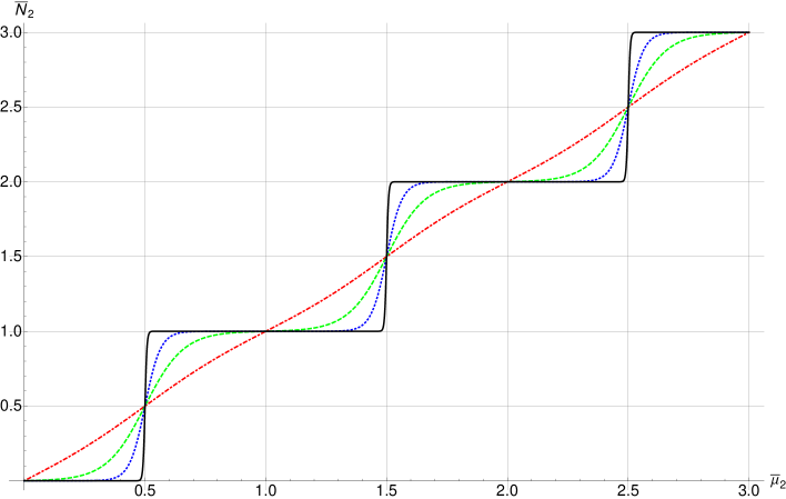
Figure 1: For $f=2$, plot of $\bar{N}_{2}$ as a function of $\bar{\mu}_{2}$ for $\tau=1.5$ (red, dotdashed), $\tau=0.5$ (green, dashed), $\tau=0.2$ (blue, dotted), and $\tau=0.025$ (black, solid).

If a system at high temperature is described in the path-integral formalism by fluctuations (as a function of the two Euclidean spacetime coordinates) of $\bar{N}_{2}$ around a half-integer value, the corresponding system at zero temperature will have two coexisting phases (fluctuations are amplified when $\tau$ is decreased). On the other hand, away from the phase boundaries, the system will become uniform at zero temperature (fluctuations are damped when $\tau$ is decreased). Fig. 2 shows spatial inhomogeneities develop in a system with $\bar{\mu}_{2}$ chosen at the phase boundary as it is cooled and Fig. 3 shows thermal fluctuations dying down in a system with $\bar{\mu}_{2}$ chosen away from the phase boundary. The square grid with many cells can either be thought of as an Euclidean spacetime grid or a sampling of several identical systems (in terms of the choice of $\bar{\mu}_{2}$ and $\tau$).

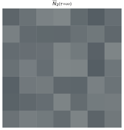
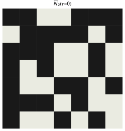
Figure 2: For $f=2$, a spacetime grid with small fluctuations around $\bar{N}_{2}=1/2$ at large $\tau$ (left panel) results in two coexisting phases (characterized by $\bar{N}_{2}=0$ and $\bar{N}_{2}=1$) at zero temperature (right panel).

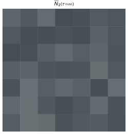
Figure 3: For $f=2$, a spacetime grid with random fluctuations around $\bar{N}_{2}=2/5$ at large $\tau$ (left panel) results in a uniform particle number ($\bar{N}_{2}=0$) at $\tau=0$ (right panel).

III.2 Phase structure for $f=3$

We determine the phase boundaries, separating cells with different $(\bar{N}_{2},\bar{N}_{3})$ as described in Sec. II.3. As explained in Sec. II.3 it is also instructive to use a different coordinate system for the chemical potentials, obtained from $(\mu_{1},\mu_{2},\mu_{3})$ by an orthonormal transformation:

$$\begin{pmatrix}\tilde{\mu}_{1}\\ \tilde{\mu}_{2}\\ \tilde{\mu}_{3}\end{pmatrix}=\begin{pmatrix}\frac{1}{\sqrt{3}}&\frac{1}{\sqrt{3}}&\frac{1}{\sqrt{3}}\\ \frac{1}{\sqrt{2}}&-\frac{1}{\sqrt{2}}&0\\ \frac{1}{\sqrt{6}}&\frac{1}{\sqrt{6}}&-\frac{2}{\sqrt{6}}\\ \end{pmatrix}\begin{pmatrix}\mu_{1}\\ \mu_{2}\\ \mu_{3}\end{pmatrix}\,,$$ (46)

i.e., $\tilde{\mu}_{2}=\bar{\mu}_{2}/\sqrt{2}$ and $\tilde{\mu}_{3}=(-\bar{\mu}_{2}+2\bar{\mu}_{3})/\sqrt{6}$. We denote the corresponding particle numbers by $\tilde{N}_{2}$ and $\tilde{N}_{3}$. An alternative representation of the partition function, which simplifies the determination of vertices in terms of the coordinates $\tilde{\mu}_{i}$, is given in appendix A. In these coordinates, the phase structure is symmetric under rotations by $\pi/3$ and composed of two types of hexagonal cells, a central regular hexagon is surrounded by six smaller non-regular hexagons, which are identical up to rotations. Figure 4 shows the phase boundaries at zero temperature in both coordinate systems.

The condition on the integers ${\boldsymbol{m}}$ as given in (40) reduce to $m_{3}=m_{2}-m_{1}$ and $m_{4}=-\frac{3}{2}m_{2}$. Therefore, we require $m_{2}$ to be even and write it as $2l_{2}$. From Eq. (41) we see that the boundaries in the $(\bar{\mu}_{2},\bar{\mu}_{3})$ plane are periodic under shifts

$$\begin{pmatrix}\bar{\mu}^{\prime}_{2}\\ \bar{\mu}^{\prime}_{3}\end{pmatrix}=\begin{pmatrix}\bar{\mu}_{2}\\ \bar{\mu}_{3}\end{pmatrix}+m_{1}\begin{pmatrix}2\\ 1\end{pmatrix}-l_{2}\begin{pmatrix}1\\ -1\end{pmatrix}\qquad\qquad m_{1},\,l_{2}\in\mathbb{Z}\,.$$ (47)

The shift symmetry (47) is obvious in Fig. 4.

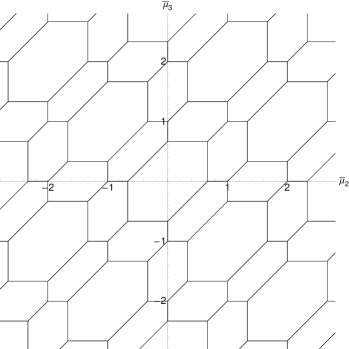
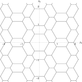
Figure 4: Phase boundaries at zero temperature for $f=3$ in the $\bar{\mu}$ plane (left) and the $\tilde{\mu}$ plane (right).

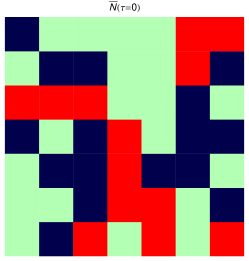
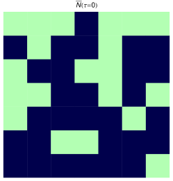
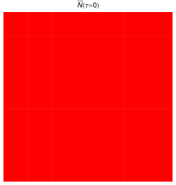
Figure 5: Left panel shows, for $f=3$, the result of cooling a spacetime grid with random fluctuations around $\bar{N}\equiv(\bar{N}_{2},\bar{N}_{3})=(\frac{2}{3},\frac{2}{3})$ at large $\tau$ to $\tau=0$, where three phases coexist: $\bar{N}=(0,0)$ (red squares), $\bar{N}=(\frac{1}{2},1)$ (dark-blue squares), and $\bar{N}=(1,\frac{1}{2})$ (light-green squares). Center panel shows result starting from $\bar{N}=(\frac{3}{4},\frac{3}{4})$ at high $\tau$, which results in two coexisting phases ($\bar{N}=(\frac{1}{2},1)$ and $\bar{N}=(1,\frac{1}{2})$) at $\tau=0$. Right panel shows results starting from $\bar{N}=(\frac{1}{2},\frac{1}{2})$ at high $\tau$, resulting in a single phase (characterized by $\bar{N}=(0,0)$) at $\tau=0$.

All $\bar{\mu}$’s inside a given hexagonal cell result in identical $\bar{N}$ as $\tau\to 0$, given by the coordinates of the center of the cell. For example, $\bar{\mu}$’s in the central hexagonal cell lead to $\bar{N}_{2,3}=(0,0)$ at $\tau=0$, the six surrounding cells are characterized by $\bar{N}_{2,3}=\pm(1,\frac{1}{2})$, $\bar{N}_{2,3}=\pm(\frac{1}{2},1)$, and $\bar{N}_{2,3}=\pm(-\frac{1}{2},\frac{1}{2})$. Every vertex is common to three cells. The coordinates of the vertices between the central cell and the six surrounding cells are $\pm(\frac{2}{3},\frac{2}{3})$, $\pm(0,\frac{2}{3})$, $\pm(\frac{2}{3},0)$, $\pm(1,1)$, $\pm(0,1)$, $\pm(1,0)$. All other vertices in the $\bar{\mu}$ plane can be generated by shifts of the form (47).

First-order phase transitions occur between neighboring cells with different particle numbers $\bar{N}_{2,3}$ at $\tau=0$. At the edges of the hexagonal cells, two phases can coexist, and at the vertices, three phases can coexist at zero temperature.

In analogy to the two-flavor case (cf. Fig. 2), a high-temperature system with small fluctuations (as a function of Euclidean spacetime) of $\bar{\mu}_{2,3}$ can result in two or three phases coexisting or result in a pure state as $\tau\to 0$ depending on the choice of $\bar{\mu}_{2,3}$ (see Fig. 5 for examples of all three cases). Figure 6 shows the flow of $(\tilde{N}_{3}(\tau),\tilde{N}_{2}(\tau))$ from $\tau=\infty$ to $\tau=0$ at fixed $(\tilde{\mu}_{3},\tilde{\mu}_{2})=(\tilde{N}_{3}(\tau=\infty),\tilde{N}_{2}(\tau=\infty))$. The zero-temperature limit $(\tilde{N}_{3}(0),\tilde{N}_{2}(0))$ is given by the coordinates of the center of the respective hexagonal cell.

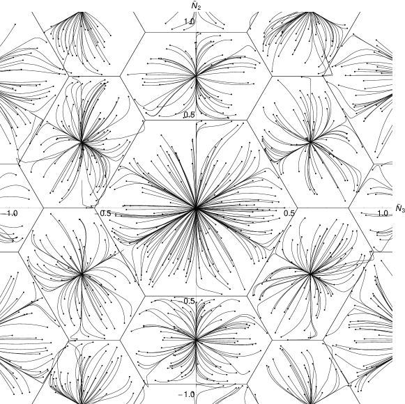
Figure 6: Visualization of the $\tilde{N}$ evolution with decreasing $\tau$ starting from randomly scattered initial points at $\tau=\infty$ (indicated by dots in the plot).

III.3 f=4

We use Eq. (34) to identify the phase structure in the $(\bar{\mu}_{2},\bar{\mu}_{3},\bar{\mu}_{4})$ space, which is divided into three-dimensional cells characterized by identical particle numbers $\bar{N}_{2,3,4}$ at zero temperature. At the boundaries of these cells, multiple phases can coexist at zero temperature (see Fig. 7 for examples). We find different types of vertices (corners of the cells), where four and six phases can coexist. At all edges, three phases can coexist.

We set $l_{1}=m_{1}+m_{2}-m_{3}$, $l_{2}=m_{1}$ and $l_{3}=m_{2}$. From Eq. (41) for $f=4$, we see that the phase structure is periodic under

$$\begin{pmatrix}\bar{\mu}_{2}\\ \bar{\mu}_{3}\\ \bar{\mu}_{4}\end{pmatrix}\rightarrow\begin{pmatrix}\bar{\mu}_{2}\\ \bar{\mu}_{3}\\ \bar{\mu}_{4}\end{pmatrix}+l_{1}\begin{pmatrix}1\\ 1\\ 0\end{pmatrix}+l_{2}\begin{pmatrix}1\\ 0\\ 1\end{pmatrix}+l_{3}\begin{pmatrix}0\\ 1\\ 1\end{pmatrix}\qquad\qquad l_{1,2,3}\in\mathbb{Z}\,.$$ (48)

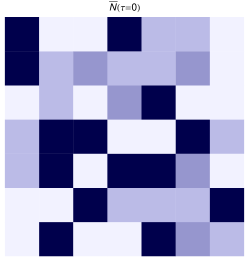
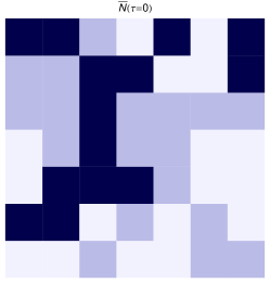
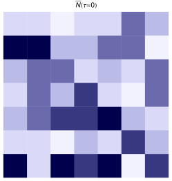
Figure 7: Left panel shows, for $f=4$, the result of cooling a spacetime grid with random fluctuations around $\bar{N}\equiv(\bar{N}_{2},\bar{N}_{3},\bar{N}_{4})=(\frac{3}{4},\frac{3}{4},\frac{3}{4})$ at large $\tau$ to $\tau=0$, where four phases coexist: $\bar{N}=(0,0,0)$, $\bar{N}=(\frac{1}{2},\frac{1}{2},1)$, $\bar{N}=(\frac{1}{2},1,\frac{1}{2})$, and $\bar{N}=(1,\frac{1}{2},\frac{1}{2})$. Different colors are assigned to different phases. Center panel shows result starting from $\bar{N}=(\frac{7}{8},\frac{7}{8},\frac{7}{8})$ at high $\tau$, which results in three coexisting phases ($\bar{N}=(\frac{1}{2},\frac{1}{2},1)$, $\bar{N}=(\frac{1}{2},1,\frac{1}{2})$, and $\bar{N}=(1,\frac{1}{2},\frac{1}{2})$) at $\tau=0$. Right panel shows results starting from $\bar{N}=(1,1,1)$ at high $\tau$, resulting in six coexisting phases characterized by $\bar{N}=(\frac{1}{2},\frac{1}{2},1)$, $\bar{N}=(\frac{1}{2},1,\frac{1}{2})$, $\bar{N}=(1,\frac{1}{2},\frac{1}{2})$, $\bar{N}=(\frac{3}{2},\frac{3}{2},1)$, $\bar{N}=(\frac{3}{2},1,\frac{3}{2})$, and $\bar{N}=(1,\frac{3}{2},\frac{3}{2})$.

As in the three flavor case, we observe that the phase structure exhibits higher symmetry in coordinates $\tilde{\mu}$ which are related to $\mu$ through an orthonormal transformation. A particularly convenient choice for $f=4$ turns out to be given by

$$\begin{pmatrix}\tilde{\mu}_{1}\\ \tilde{\mu}_{2}\\ \tilde{\mu}_{3}\\ \tilde{\mu}_{4}\end{pmatrix}=\frac{1}{2}\begin{pmatrix}1&1\\ 1&-1\end{pmatrix}\otimes\begin{pmatrix}1&1\\ 1&-1\end{pmatrix}\begin{pmatrix}\mu_{1}\\ \mu_{2}\\ \mu_{3}\\ \mu_{4}\end{pmatrix}\,,$$ (49)

since the phase structure becomes periodic under shifts parallel to the coordinate axes:

$$\begin{pmatrix}\tilde{\mu}_{2}\\ \tilde{\mu}_{3}\\ \tilde{\mu}_{4}\end{pmatrix}\rightarrow\begin{pmatrix}\tilde{\mu}_{2}\\ \tilde{\mu}_{3}\\ \tilde{\mu}_{4}\end{pmatrix}+l_{1}\begin{pmatrix}0\\ 0\\ 1\end{pmatrix}+l_{2}\begin{pmatrix}1\\ 0\\ 0\end{pmatrix}+l_{3}\begin{pmatrix}0\\ 1\\ 0\end{pmatrix}\qquad\qquad l_{1,2,3}\in\mathbb{Z}$$ (50)

as obtained from Eq. (48). An alternative representation of the partition function in these coordinates is given in Eq. (61). At zero temperature the $\tilde{\mu}_{2,3,4}$ space is divided into two types of cells which are characterized by identical particle numbers (see Fig. 8 for visualizations). We can think of the first type as a cube (centered at the origin, with side lengths 1 and parallel to the coordinate axes) where all the edges have been cut off symmetrically. The original faces are reduced to smaller squares (perpendicular to the coordinate axes) with corners at $\tilde{\mu}_{2,3,4}=(\pm\frac{1}{2},\pm\frac{1}{4},\pm\frac{1}{4})$ (permutations and sign choices generate the six faces). This determines the coordinates of the remaining 8 corners to be located at $(\pm\frac{3}{8},\pm\frac{3}{8},\pm\frac{3}{8})$. The shift symmetry (50) tells us that these “cubic” cells are stacked together face to face. The remaining space (around the edges of the original cube) is filled by cells of the second type (in the following referred to as “edge” cells), which are identical in shape and are oriented parallel to the three coordinate axes.

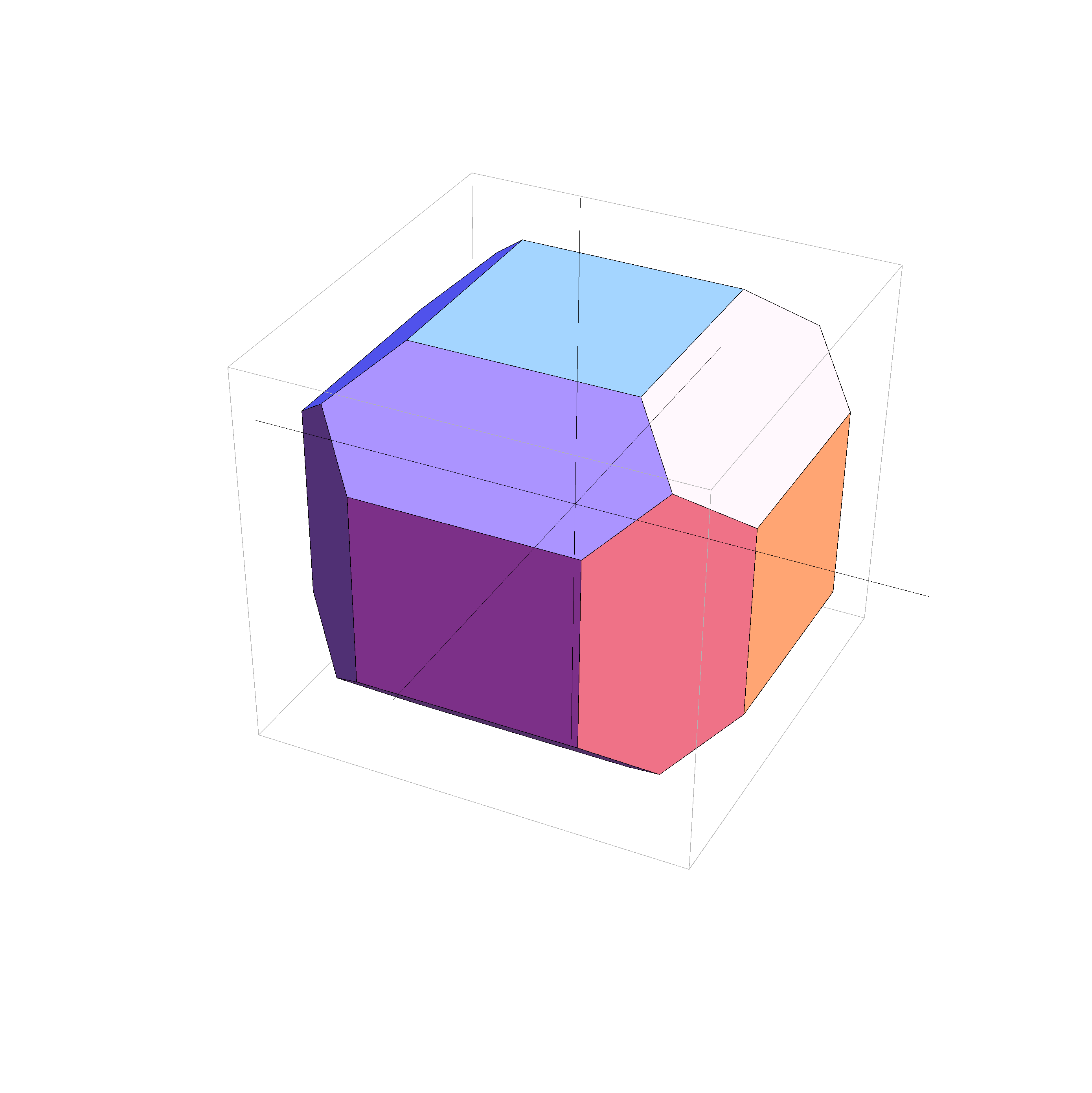
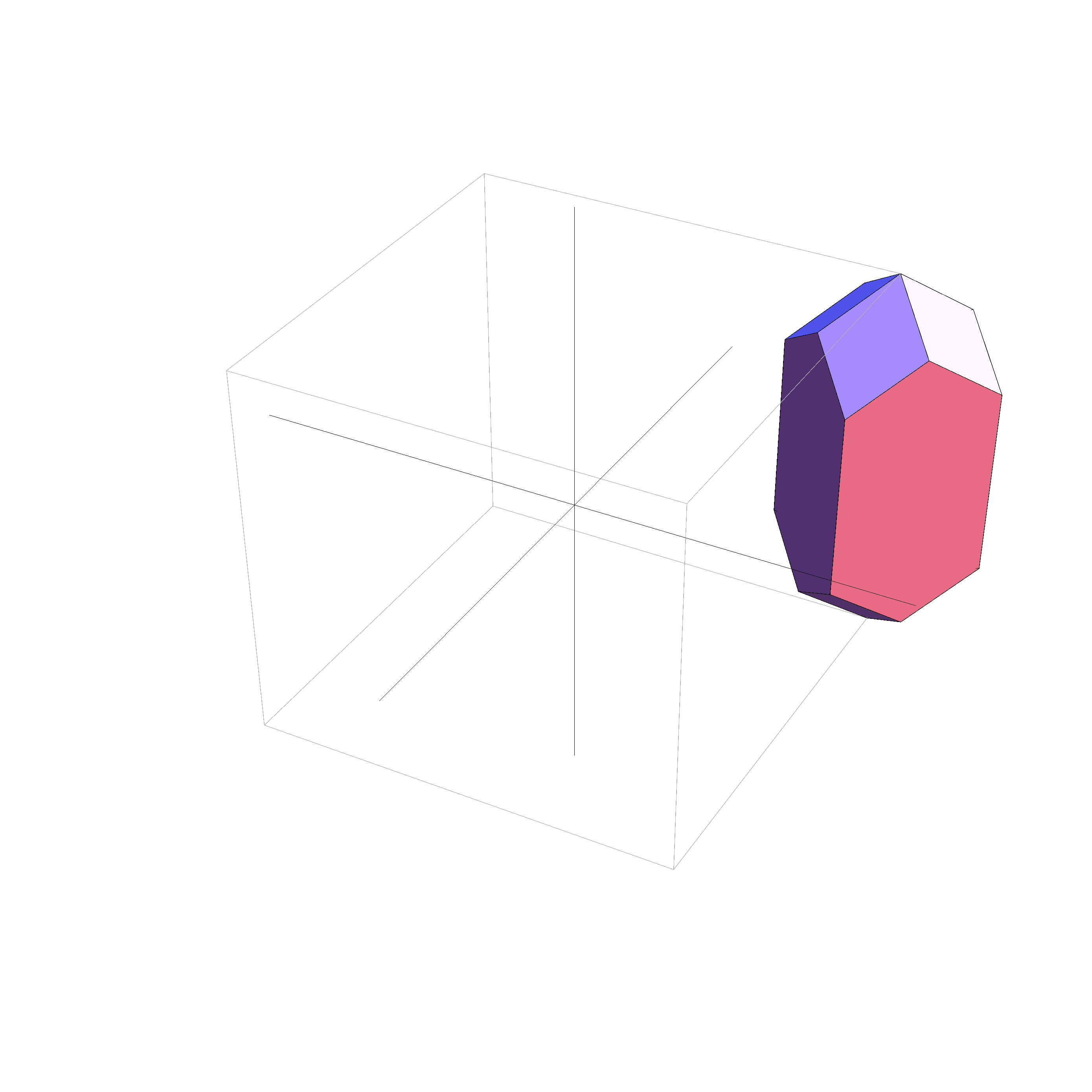
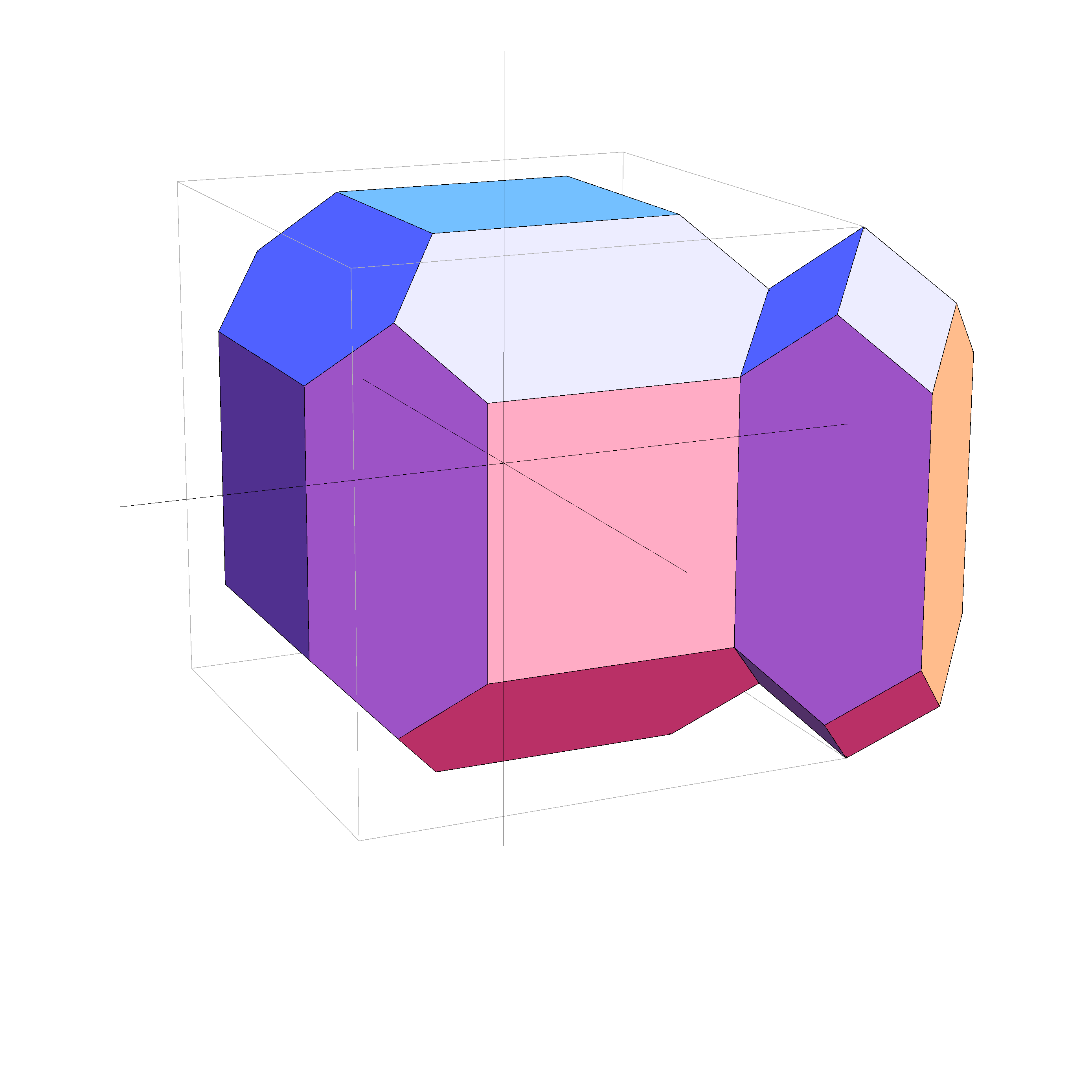
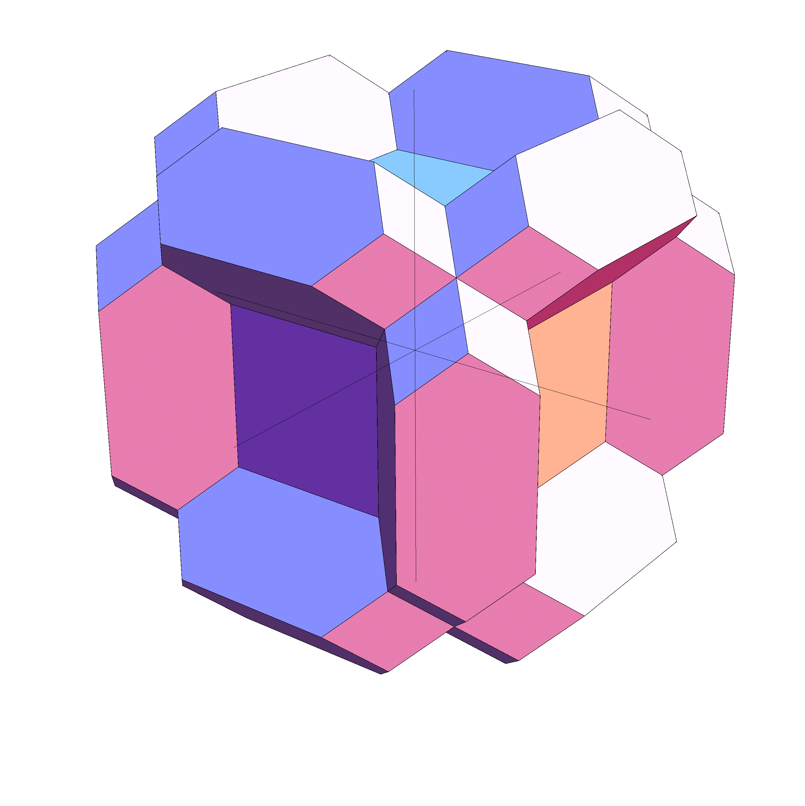
Figure 8: Cells defining the zero-temperature phase structure for $f=4$ in the $\tilde{\mu}$ coordinates as described in the text. The top left figure shows the central “cubic” cell, the top right figure a single “edge” cell. The bottom right figure shows the cubic cell together with all 12 attaching edge cells.

This leads to different kinds of vertices (at the corners of the cells described above) where multiple phases can coexist at zero temperature. There are corners which are common points of two cubic and two edge cells (coexistence of 4 phases, for example at $(\pm\frac{1}{2},\pm\frac{1}{4},\pm\frac{1}{4})$), there are corners which are common points of one cubic and three edge cells (coexistence of 4 phases, for example at $(\pm\frac{3}{8},\pm\frac{3}{8},\pm\frac{3}{8})$), and there are corners which are common points of six edge cells (coexistence of six phases, for example at $\tilde{\mu}_{2,3,4}=(\pm\frac{1}{2},\pm\frac{1}{2},\pm\frac{1}{2})$. Any edge between two of these vertices is common to three cells.

III.4 Phase structure for $f>4$

For $f=3$ and $f=4$, we find that the coordinates $(\bar{\mu}_{2},\ldots,\bar{\mu}_{f})$ of all vertices (corners of the cells in the $\bar{\mu}$ space resulting in identical particle numbers at zero temperature) are multiples of $\frac{1}{f}$. In general, two special vertices are located at $\bar{\mu}_{i}=1$ for all $2\leq i\leq f$ and $\bar{\mu}_{i}=1-\frac{1}{f}$ for all $2\leq i\leq f$.

If $\bar{\mu}_{i}=1-\frac{1}{f}$ for all $2\leq i\leq f$, we find that $f$ phases can coexist at zero temperature. These have particle numbers $\bar{N}_{2,\ldots,f}=(0,\ldots,0)$ and all $(f-1)$ distinct permutations of $(1,\frac{1}{2},\ldots,\frac{1}{2})$.

If $\bar{\mu}_{i}=1$ for all $2\leq i\leq f$, we find that $f\choose 2$ phases can coexist at zero temperature. The corresponding particle numbers are given by the $(f-1)$ distinct permutations of $(1,\frac{1}{2},\ldots,\frac{1}{2})$ and the $f-1\choose 2$ distinct permutations of $(\frac{3}{2},\frac{3}{2},1,\ldots,1)$.

While for $f=5$, we find only up to $5\choose 2$ coexisting phases, we find up to $6\choose 3$ coexisting phases for $f=6$ (for example at $\bar{\mu}_{2,\ldots,6}=(1,\frac{1}{2},0,0,0)$). We also find up to $8\choose 4$ coexisting phases for $f=8$ (for example at $\bar{\mu}_{2,\ldots,8}=(1,1,1,1,1,1,0)$). This leads us to conjecture that the maximal number of coexisting phases is given by $f\choose{\lfloor f/2\rfloor}$, increasing exponentially for large $f$.

IV Conclusions

Multiflavor QED in two dimensions with flavor-dependent chemical potentials exhibits a rich phase structure at zero temperature. We studied massless multiflavor QED on a two-dimensional tours. The system is always in a state with a net charge of zero in the Euclidean formalism due to the integration over the toron variables. The toron variables completely dominate the dependence on the chemical potentials and the resulting partition function has a representation in the form of a multidimensional theta function. We explicitly worked out the two-dimensional phase structure for the three flavor case and the three-dimensional phase structure for the four flavor case. The different phases at zero temperature are characterized by certain values of the particle numbers and separated by first-order phase transitions. We showed that two or three phases can coexist in the case of three flavors. We also showed that two, three, four and six phases can coexist in the case of four flavors. Based on our exhaustive studies of the three and four flavor case and an exploratory investigation of the five, six, and eight flavor case we conjecture that up to $f\choose{\lfloor f/2\rfloor}$ phases can coexist in a theory with $f$ flavors.

Appendix A Alternative representations of the partition function

There are many equivalent representations of the partition function $Z_{t}(\mbox{\boldmath$\mu$},\tau)$, related by variable changes of the integer summation variables in (5), (6) or (34). Here we present the result obtained by an orthonormal variable change at the level of Eq. (5), splitting the chemical potentials $\mu_{1},\ldots,\mu_{f}$ in one flavor-independent and $(f-1)$ traceless components according to

$$\tilde{\mu}_{1} =\frac{1}{\sqrt{f}}\sum_{i=1}^{f}\mu_{i}\,,$$ (51)

$$\tilde{\mu}_{j} =\frac{1}{\sqrt{j(j-1)}}\left(\sum_{i=1}^{j-1}\mu_{i}-(j-1)\mu_{j}\right)\,,\qquad 2\leq j\leq f\,.$$ (52)

The induced variable change in the $2f$ integer summation variables in Eq. (5) is non-trivial and requires successive transformations of the form

$$\sum_{k,l=-\infty}^{\infty}f(k-l,Mk+l)=\sum_{q=0}^{M}\sum_{m,n=-\infty}^{\infty}f((M+1)m+q,(M+1)n-q)\,,\qquad M\in\mathbb{N}_{+}\,.$$ (53)

In this way, it is possible to write the partition function as a product of $2f-2$ one-dimensional theta functions, where $f-1$ factors are independent of the chemical potentials and each one of the other $f-1$ factors depends only on a single traceless chemical potential $\tilde{\mu}_{i}$ (with $2\leq i\leq f$). However, the arguments of the theta functions are not independent since they involve a number of finite summation variables resulting from variable changes of the form (53) and the partition function does not factorize. The final result reads

$$Z_{t}(\mbox{\boldmath$\mu$},\tau) \propto\left(\prod_{j=1}^{f}\sum_{k_{j}=0}^{1}\right)\left(\prod_{j=2}^{f}\sum_{q_{j}=0}^{j-1}\sum_{p_{j}=0}^{j-1}\right)\delta_{0,\left(2\sum_{j=2}^{f}p_{j}+\sum_{j=1}^{f}k_{j}\right)\,\text{mod}\,2f}$$ (54)

$$\quad\times\left[\prod_{j=2}^{f}h_{2\tau j(j-1)}\left(\frac{1}{j(j-1)}\sum_{i=2}^{j-1}q_{i}-\frac{1}{j}q_{j}+\frac{1}{\sqrt{j(j-1)}}\left(\frac{\tilde{k}_{j}}{2}-\frac{i}{\tau}\tilde{\mu}_{j}\right)\right)\right]$$ (55)

$$\quad\times\left[\prod_{j=2}^{f}h_{2\tau j(j-1)}\left(\frac{1}{j(j-1)}\sum_{i=2}^{j-1}p_{i}-\frac{1}{j}p_{j}+\frac{1}{\sqrt{j(j-1)}}\frac{\tilde{k}_{j}}{2}\right)\right]\,,$$ (56)

where $\tilde{k}_{j}=\frac{1}{\sqrt{j(j-1)}}\left(\sum_{i=1}^{j-1}k_{i}-(j-1)k_{j}\right)$ and

$$h_{\alpha}(z)\equiv\sum_{n=-\infty}^{\infty}e^{-\pi\alpha(n+z)^{2}}\,.$$ (57)

Permuting indices in variable changes of the form (52) shows that the $(f-1)$-dimensional finite sum $\prod_{j}\sum_{p_{j}}$ will result in an expression that depends only on $\sum_{j=1}^{f}k_{j}$.

To study the zero-temperature properties, we can apply the Poisson summation formula for each factor of $h_{\alpha}(z)$ in Eq. (54).

A.1 Explicit form for $f=3$

For $f=3$, the Poisson-resummed version of (54) can be simplified to

$$Z_{t}(\mbox{\boldmath$\mu$},\tau) \propto\sum_{m_{1},m_{2},l_{1},l_{2}=-\infty}^{\infty}\delta_{0,\left(m_{1}+l_{2}\right)\,\text{mod}\,2}\,\delta_{0,\left(m_{2}+l_{1}\right)\,\text{mod}\,2}\,\,e^{-\frac{\pi}{4\tau}\left((m_{1}+m_{2})^{2}+3(m_{1}-m_{2})^{2}+(l_{1}+l_{2})^{2}+\frac{1}{3}(l_{1}-l_{2})^{2}\right)}$$ (58)

$$\quad\times e^{\frac{\pi}{\tau}\left((m_{1}+m_{2})\sqrt{2}\tilde{\mu}_{2}+(m_{1}-m_{2})\sqrt{6}\tilde{\mu}_{3}\right)}\,.$$ (59)

For $\tau\to 0$, the sums over $l_{1,2}$ become trivial and we obtain

$$Z_{t}(\mbox{\boldmath$\mu$},\tau)\rightarrow\sum_{m_{1},m_{2}=-\infty}^{\infty}e^{-\frac{\pi}{\tau}\left(\frac{1}{4}(m_{1}+m_{2})^{2}+\frac{3}{4}(m_{1}-m_{2})^{2}-(m_{1}+m_{2})\sqrt{2}\tilde{\mu}_{2}+(m_{1}-m_{2})\sqrt{6}\tilde{\mu}_{3}+\frac{1}{3}\left(1-\delta_{0,m_{1}\text{mod}2}\delta_{0,m_{2}\text{mod}2}\right)\right)}\,.$$ (60)

The particle numbers $\tilde{N}_{2}$ and $\tilde{N}_{3}$ at zero temperature are determined by those integer pairs $(m_{1},m_{2})$ dominating the sum in Eq. (60). Compared to the general expression in Eq. (34), we have reduced the number of summation variables from four to two, which simplifies the search for vertices where multiple phases coexist. Furthermore, there is a one-to-one map from $(\tilde{N}_{2},\tilde{N}_{3})$ to $(m_{1},m_{2})$ inside any given cell in the zero-temperature phase-structure. Once we have located neighboring cells in terms of $(m_{1},m_{2})$, we can immediately read off the $\tilde{\mu}_{2,3}$ coordinates of the corresponding vertices/edges between them (by requiring that the contributions to the sum (60) are identical).

A.2 Explicit form for $f=4$

Following the general procedure described above, we can write the partition function for $f=4$ in the coordinates defined in Eq. (49) as

$$Z_{t}(\mbox{\boldmath$\mu$},\tau)\propto\sum_{m_{2},m_{3},m_{4},n_{2},n_{3},n_{4}=-\infty}^{\infty}\delta_{0,(m_{2}+m_{3}+m_{4})\,\text{mod}\,2}\,\delta_{0,(m_{2}+n_{2}+n_{3})\,\text{mod}\,2}\,\delta_{0,(m_{3}+n_{3}+n_{4})\,\text{mod}\,2}\,\,e^{-\frac{\pi}{2\tau}\sum_{j=2}^{4}\left(m_{j}^{2}+n_{j}^{2}-4m_{j}\tilde{\mu}_{j}\right)}\,.$$ (61)

Similarly to the three flavor case, the sum over $n_{2,3,4}$ becomes trivial in the $\tau\to 0$ limit, depending only on $m_{2}\,\text{mod}\,2$ and $m_{3}\,\text{mod}\,2$. The remaining summation variables $m_{2,3,4}$ directly determine the particle numbers in the different phases at zero temperature and the vertices can be found analogously to the three flavor case.

- (1) I. Sachs, A. Wipf and A. Dettki, Phys. Lett. B 317, 545 (1993) [hep-th/9308130].
- (2) I. Sachs and A. Wipf, Annals Phys. 249, 380 (1996) [hep-th/9508142].
- (3) I. Sachs and A. Wipf, Helv. Phys. Acta 65, 652 (1992) [arXiv:1005.1822 [hep-th]].
- (4) D. J. Gross, R. D. Pisarski and L. G. Yaffe, Rev. Mod. Phys. 53, 43 (1981).
- (5) R. Narayanan, Phys. Rev. D 86, 087701 (2012) [arXiv:1206.1489 [hep-lat]].
- (6) R. Narayanan, Phys. Rev. D 86, 125008 (2012) [arXiv:1210.3072 [hep-th]].
- (7) B. Deconinck, Chapter 21 in F.W.J. Olver, D.M. Lozier, R.F. Boisvert, et.al., NIST Handbook of Mathematical Functions, Cambridge University Press, ISBN 978-0521192255, MR2723248.