Symmetric multivariate polynomials
as a basis for three-boson light-front wave functions

Abstract

We develop a polynomial basis to be used in numerical calculations of light-front Fock-space wave functions. Such wave functions typically depend on longitudinal momentum fractions that sum to unity. For three particles, this constraint limits the two remaining independent momentum fractions to a triangle, for which the three momentum fractions act as barycentric coordinates. For three identical bosons, the wave function must be symmetric with respect to all three momentum fractions. Therefore, as a basis, we construct polynomials in two variables on a triangle that are symmetric with respect to the interchange of any two barycentric coordinates. We find that, through the fifth order, the polynomial is unique at each order, and, in general, these polynomials can be constructed from products of powers of the second and third-order polynomials. The use of such a basis is illustrated in a calculation of a light-front wave function in two-dimensional $\phi^{4}$ theory; the polynomial basis performs much better than the plane-wave basis used in discrete light-cone quantization.

I Introduction

Light-front quantization Dirac ; DLCQreview is a natural choice for the nonperturbative solution of a quantum field theory. The eigenstates are built as expansions in terms of Fock states, states of definite particle number and definite momentum, where the coefficients are boost-invariant wave functions. The vacuum state is simply the Fock vacuum, thereby giving the wave functions a standard, quantum mechanical interpretation.

The light-front time coordinate is chosen to be $x^{+}\equiv t+z/c$, and the corresponding light-front spatial coordinate is $x^{-}\equiv t-z/c$; the other spatial coordinates are unchanged. The conjugate light-front energy is $p^{-}=E-cp_{z}$, and the light-front longitudinal momentum is $p^{+}=E/c+p_{z}$. A boost-invariant momentum fraction $x_{i}=p_{i}^{+}/P^{+}$ is defined for the ith particle with momentum $p_{i}^{+}$ in a system with total momentum $P^{+}$. Because the light-front longitudinal momentum is always positive, these momentum fractions are between zero and one. Also, momentum conservation dictates that they sum to one.

In the three-particle case, the three momentum fractions correspond to the barycentric coordinates of a triangle. Any two can be treated as the independent variables. For a wave function that describes three identical bosons, there must be symmetry under the interchange of any two of the three coordinates, not just symmetry under the interchange of the two chosen as independent. Any set of basis functions to be used in numerical approximations of such a wave function should share this symmetry. However, the usual treatment of two-variable polynomials on a triangle is limited to consideration of symmetry with respect to only the two independent variables sympoly ; multpoly . Here we consider the full-symmetry constraint.

We find that full symmetry among all three barycentric coordinates dramatically reduces the number of polynomials at any given order. For the lowest orders, there is only one; at the sixth order, there are two. In general, for polynomials of order $N$, the number of linearly independent polynomials is the number of combinations of two nonnegative integers $n$ and $m$ such that $N=2n+3m$. These polynomials can be chosen to be products of $n$ factors of the second-order polynomial and $m$ factors of the third-order polynomial. They are not orthonormal, but given such a set of polynomials one can, of course, systematically generate an orthonormal set.

As a test of the utility of these polynomials, we consider a problem in two-dimensional $\phi^{4}$ theory where the mass of the eigenstate is shifted by coupling between the one-boson sector and the three-boson sector. The results obtained are quite encouraging. For comparison we also consider discrete light-cone quantization (DLCQ) PauliBrodsky ; DLCQreview which uses a periodic plane-wave basis and therefore quadratures in momentum space that use equally spaced points. The DLCQ results would require extrapolation to obtain an accurate answer, whereas the symmetric-polynomial basis immediately converges.

The content of the remainder of the paper is as follows. In Sec. II, we specify the construction of the fully symmetric polynomials. The first subsection describes the lowest order cases, where a first-order polynomial is found to be absent and the second and third-order polynomials are found to be unique. The second subsection gives the analysis at any finite order, with details of a proof left to an Appendix. The illustration of the use of these polynomials, as a basis for the three-boson wave function in $\phi^{4}$ theory, is presented in Sec. III. A brief summary is given in Sec. IV.

II Fully symmetric polynomials

II.1 Lowest orders

We consider polynomials in Cartesian coordinates $x$ and $y$, on the triangle defined by

$$0\leq x\leq 1,\;\;0\leq y\leq 1,\;\;0\leq 1-x-y\leq 1,$$ (1)

that are fully symmetric with respect to interchange of the coordinates $x$, $y$, and $z=1-x-y$. These can be viewed as the restriction of three-variable polynomials on the unit cube to the plane $x+y+z=1$. The construction of the fully symmetric three-variable polynomials on the cube is trivial; at order $N$, the possible polynomials are linear combinations of the form

$$x^{i}y^{j}z^{k}+x^{j}y^{k}z^{i}+x^{k}y^{i}z^{j}+x^{j}y^{i}z^{k}+x^{i}y^{k}z^{j}+x^{k}y^{j}z^{i},$$ (2)

with $i$, $j$, and $k$ nonnegative integers such that $N=i+j+k$. The linearly independent polynomials would correspond to some particular ordering of these indices, such as $i\leq j\leq k$. For $N=0$ or 1 there is only one polynomial, but for $N\geq 2$ there are several.

The restriction to the plane defined by $x+y+z=1$ is, however, a severe constraint. As we will see, the fully symmetric two-variable polynomials are unique up through $N=5$. For $N=1$, the constraint eliminates the only candidate; the restriction from the cube to the plane makes $x+y+z$ just a constant. For $N=2$, we have two candidates

$$x^{2}+y^{2}+z^{2}\;\;\mbox{and}\;\;xy+xz+yz.$$ (3)

Substitution of $z=1-x-y$ quickly shows that they are equivalent up to terms of order less than two. Similarly, for $N=3$, the three candidates

$$x^{3}+y^{3}+z^{3},\;\;x^{2}y+x^{2}z+xy^{2}+xz^{2}+y^{2}z+yz^{2},\;\;\mbox{and}\;\;xyz$$ (4)

reduce to equivalent polynomials, up to terms of order less than three, upon substitution of $z=1-x-y$. Equivalence does not exclude the possibility that the polynomials will differ by fully symmetric polynomials of lower order. The terms of order three are the same, and the polynomials differ by at most symmetric polynomials of lower order.

To proceed in this fashion to higher orders is, of course, possible but tedious. Instead we develop a direct analysis of the possible two-variable polynomials and the symmetry constraints, as described in the next subsection.

II.2 General analysis

In order to avoid complications due to lower-order contributions, we first change variables from $x,y,z$ to $u,v,w$ defined by

$$u=x-1/3,\;\;v=y-1/3,\;\;w=z-1/3=-(u+v).$$ (5)

Any polynomial $P$ on the triangle, for which each term is of order $N$, can be written in the form

$$P(u,v)=\sum_{n=0}^{N}c_{n}u^{n}v^{N-n},$$ (6)

and, unlike replacement of $x$ or $y$ by $z=1-x-y$, powers of $w=-(u+v)$ that appear in replacements of $u$ or $v$ do not introduce lower-order contributions.

Symmetry with respect to just $u$ and $v$ restricts the coefficients to be such that $c_{n}=c_{N-n}$. If symmetry with respect to $v\rightarrow w=-(u+v)$ is imposed, the coefficients must satisfy the constraint

$$\sum_{n=0}^{N}c_{n}u^{N-n}v^{n}=\sum_{n=0,N}c_{n}u^{N-n}(-1)^{n}(u+v)^{n}=\sum_{n=0}^{N}c_{n}u^{N-n}(-1)^{n}\sum_{m=0}^{n}\left(\begin{array}[]{c}n\\ m\end{array}\right)u^{n-m}v^{m}.$$ (7)

These are sufficient to guarantee that the resulting polynomial has all the desired symmetries.

The symmetry conditions can be reduced to a linear system for the coefficients. With a change in the order of the sums on the right of (7) and an interchange of the summation indices $m$ and $n$, we find

$$\sum_{n=0}^{N}c_{n}u^{N-n}v^{n}=\sum_{n=0}^{N}\sum_{m=n}^{N}(-1)^{m}\left(\begin{array}[]{c}m\\ n\end{array}\right)c_{m}u^{N-n}v^{n}.$$ (8)

Therefore, the coefficients must satisfy the linear system

$$c_{n}=c_{N-n},\;\;\sum_{m=n}^{N}(-1)^{m}\left(\begin{array}[]{c}m\\ n\end{array}\right)c_{m}=c_{n}.$$ (9)

This system may at first seem to be overdetermined, but instead it is typically underdetermined. A solution exists for any $N$ other than $N=1$. For $N=2,3,4$, and 5, there is one linearly independent solution; and, for $N\geq 6$, there can be two or more linearly independent solutions.

For example, with $N=6$ the system can be expressed in matrix form as

$$\left(\begin{array}[]{ccccccc}0&-1&1&-1&1&-1&1\\ 0&-2&2&-3&4&-5&6\\ 0&0&0&-3&6&-10&15\\ 0&0&0&-2&4&-10&20\\ 0&0&0&0&0&-5&15\\ 0&0&0&0&0&-2&6\\ 0&0&0&0&0&0&0\end{array}\right)\left(\begin{array}[]{c}c_{0}\\ c_{1}\\ c_{2}\\ c_{3}\\ c_{2}\\ c_{1}\\ c_{0}\end{array}\right)=\left(\begin{array}[]{c}0\\ 0\\ 0\\ 0\\ 0\\ 0\\ 0\end{array}\right).$$ (10)

The determinant is obviously zero, as is the case for any $N$, allowing nontrivial solutions. The system reduces to two equations

$$3c_{0}-c_{1}=0,\;\;5c_{0}-2c_{2}+c_{3}=0$$ (11)

for the four unknowns, leaving two linearly independent solutions, such as

$$u^{6}+3u^{5}v+5u^{3}v^{3}+3uv^{5}+v^{6}\;\;\mbox{and}\;\;u^{4}v^{2}+2u^{3}v^{3}+u^{2}v^{4}.$$ (12)

For any value of $N$, one finds that the number of independent solutions is always the number of ways that $N$ can be written as $2n+3m$ for nonnegative integers $n$ and $m$. A proof of this conjecture for arbitrary $N$ is given in the Appendix. Thus, in each of these cases, a fully symmetric polynomial can be chosen to be the product of $n$ copies of the second-order polynomial and $m$ copies of the third-order polynomial, or a linear combination of such polynomials. Returning to the original Cartesian coordinates, we take these two base polynomials to be

$$C_{2}(x,y)=x^{2}+y^{2}+(1-x-y)^{2}\;\;\mbox{and}\;\;C_{3}(x,y)=xy(1-x-y).$$ (13)

We then have that all fully symmetric polynomials can be constructed from linear combinations of the products

$$C_{nm}(x,y)=C_{2}^{n}(x,y)C_{3}^{m}(x,y).$$ (14)

These do not form an orthonormal set. To construct such a set, we apply the Gramm–Schmidt process, relative to the inner product

$$\int_{0}^{1}dx\int_{0}^{1-x}dyP_{n}^{(i)}(x,y)P_{m}^{(j)}(x,y)=\delta_{nm}\delta_{ij},$$ (15)

where $P_{n}^{(i)}$ is the ith polynomial of order $n$. The first few polynomials are

$$P_{0} = \sqrt{2},$$ (16)

$$P_{1} = 0,$$

$$P_{2} = \sqrt{30}\left[4x^{2}+4yx-4x+4y^{2}-4y+1\right],$$

$$P_{3} = \sqrt{3}\left[-140yx^{2}+20x^{2}-140y^{2}x+160yx-20x+20y^{2}-20y+8/3\right],$$

$$P_{4} = \sqrt{42}\left[60x^{4}+120yx^{3}-120x^{3}+180y^{2}x^{2}-200yx^{2}+80x^{2}+120y^{3}x-200y^{2}x\right.$$

$$\left.\rule{36.135pt}{0.0pt}+100yx-20x+60y^{4}-120y^{3}+80y^{2}-20y+5/3\right],$$

$$P_{5} = \sqrt{6}\left[-2310yx^{4}+210x^{4}-4620y^{2}x^{3}+5040yx^{3}-420x^{3}-4620y^{3}x^{2}+7560y^{2}x^{2}\right.$$

$$\left.\rule{36.135pt}{0.0pt}-3780yx^{2}+280x^{2}-2310y^{4}x+5040y^{3}x-3780y^{2}x+1120yx-70x\right.$$

$$\left.\rule{36.135pt}{0.0pt}+210y^{4}-420y^{3}+280y^{2}-70y+4\right],$$

$$P_{6}^{(1)} = \sqrt{\frac{10}{11863}}\left[240240x^{6}+720720yx^{5}-720720x^{5}+1441440y^{2}x^{4}-1829520yx^{4}\right.$$

$$\left.\rule{36.135pt}{0.0pt}+826980x^{4}+1681680y^{3}x^{3}-2938320y^{2}x^{3}+1709400yx^{3}-452760x^{3}\right.$$

$$\left.\rule{36.135pt}{0.0pt}+1441440y^{4}x^{2}-2938320y^{3}x^{2}+2203740y^{2}x^{2}-733320yx^{2}+120204x^{2}\right.$$

$$\left.\rule{36.135pt}{0.0pt}+720720y^{5}x-1829520y^{4}x+1709400y^{3}x-733320y^{2}x+146664yx\right.$$

$$\left.\rule{36.135pt}{0.0pt}-13944x+240240y^{6}-720720y^{5}+826980y^{4}-452760y^{3}+120204y^{2}\right.$$

$$\left.\rule{36.135pt}{0.0pt}-13944y+581\right],$$

$$P_{6}^{(2)} = \sqrt{\frac{143}{11863}}\left[-16436x^{6}-49308yx^{5}+49308x^{5}+399630y^{2}x^{4}-28140yx^{4}-50190x^{4}\right.$$

$$\left.\rule{36.135pt}{0.0pt}+881440y^{3}x^{3}-1102080y^{2}x^{3}+202440yx^{3}+18200x^{3}+399630y^{4}x^{2}\right.$$

$$\left.\rule{36.135pt}{0.0pt}-1102080y^{3}x^{2}+826560y^{2}x^{2}-155400yx^{2}-210x^{2}-49308y^{5}x-28140y^{4}x\right.$$

$$\left.\rule{36.135pt}{0.0pt}+202440y^{3}x-155400y^{2}x+31080yx-672x-16436y^{6}+49308y^{5}\right.$$

$$\left.\rule{36.135pt}{0.0pt}-50190y^{4}+18200y^{3}-210y^{2}-672y+28\right].$$

If there is only one polynomial at a particular order, the $i$ index is dropped.

III Illustration

As a sample application, we consider the integral equation for the three-boson wave function in two-dimensional $\phi^{4}$ theory. This equation is obtained from the fundamental Hamiltonian eigenvalue problem on the light front DLCQreview ,

$${\cal P}^{-}|\psi(P^{+})\rangle=\frac{M^{2}}{P^{+}}|\psi(P^{+})\rangle\;\;\mbox{and}\;\;{\cal P}^{+}|\psi(P^{+})\rangle=P^{+}|\psi(P^{+})\rangle.$$ (17)

The second equation is automatically satisfied by expanding the eigenstate in Fock states $|p_{i}^{+};P^{+},n\rangle$ of $n$ bosons with momentum $p_{i}^{+}$ such that $\sum_{i}p_{i}^{+}=P^{+}$:

$$|\psi(P^{+})\rangle=\sum_{n}(P^{+})^{(n-1)/2}\int\left(\prod_{i=1}^{n-1}dx_{i}\right)\psi_{n}(x_{1},...,x_{n})|x_{i}P^{+};P^{+},n\rangle.$$ (18)

Here $\psi_{n}$ is the $n$-boson wave function, and the factor $(P^{+})^{(n-1)/2}$ is explicit in order that $\psi_{n}$ be independent of $P^{+}$.

The light-front Hamiltonian for $\phi^{4}$ theory is

$${\cal P}^{-} = \int dp^{+}\frac{\mu^{2}}{p^{+}}a^{\dagger}(p^{+})a(p^{+})$$

$$+\frac{\lambda}{6}\int\frac{dp_{1}^{+}dp_{2}^{+}dp_{3}^{+}}{4\pi\sqrt{p_{1}^{+}p_{2}^{+}p_{3}^{+}(p_{1}^{+}+p_{2}^{+}+p_{3}^{+})}}$$

$$\rule{72.26999pt}{0.0pt}\times\left[a^{\dagger}(p_{1}^{+}+p_{2}^{+}+p_{3}^{+})a(p_{1}^{+})a(p_{2}^{+})a(p_{3}^{+})\right.$$

$$\rule{90.3375pt}{0.0pt}\left.+a^{\dagger}(p_{1}^{+})a^{\dagger}(p_{2}^{+})a^{\dagger}(p_{3}^{+})a(p_{1}^{+}+p_{2}^{+}+p_{3}^{+})\right]$$

$$+\frac{\lambda}{4}\int\frac{dp_{1}^{+}dp_{2}^{+}}{4\pi\sqrt{p_{1}^{+}p_{2}^{+}}}\int\frac{dp_{1}^{\prime+}dp_{2}^{\prime+}}{\sqrt{p_{1}^{\prime+}p_{2}^{\prime+}}}\delta(p_{1}^{+}+p_{2}^{+}-p_{1}^{\prime+}-p_{2}^{\prime+})$$

$$\rule{144.54pt}{0.0pt}\times a^{\dagger}(p_{1}^{+})a^{\dagger}(p_{2}^{+})a(p_{1}^{\prime+})a(p_{2}^{\prime+}).$$

The mass of the constituent bosons is $\mu$, and $\lambda$ is the coupling constant. The operator $a^{\dagger}(p^{+})$ creates a boson with momentum $p^{+}$; it obeys the commutation relation

$$[a(p^{+}),a^{\dagger}(p^{\prime+}]=\delta(p^{+}-p^{\prime+})$$ (20)

and builds the Fock states from the Fock vacuum $|0\rangle$ in the form

$$|x_{i}P^{+};P^{+},n\rangle=\frac{1}{\sqrt{n!}}\prod_{i=1}^{n}a^{\dagger}(x_{i}P^{+})|0\rangle.$$ (21)

The terms of the light-front Hamiltonian are such that ${\cal P}^{-}$ changes particle number not at all or by two; therefore, the number of constituents in a contribution to the eigenstate is always either odd or even.

We consider the odd case, and, to have a finite eigenvalue problem, we truncate the Fock-state expansion at three bosons. We also simplify to a problem with an exact solution by dropping from the Hamiltonian the two-body scattering term, the last term in (III). The action of the light-front Hamiltonian then yields the following coupled system of integral equations:

$$M^{2}\psi_{1} = \mu^{2}\psi_{1}+\frac{\lambda}{\sqrt{6}}\int\frac{dx_{1}dx_{2}}{4\pi\sqrt{x_{1}x_{2}x_{3}}}\psi_{3}(x_{1},x_{2},x_{3}),$$ (22)

$$M^{2}\psi_{3} = \mu^{2}\left(\frac{1}{x_{1}}+\frac{1}{x_{2}}+\frac{1}{x_{3}}\right)\psi_{3}+\frac{\lambda}{\sqrt{6}}\frac{\psi_{1}}{4\pi\sqrt{x_{1}x_{2}x_{3}}}.$$ (23)

It is understood that $x_{3}=1-x_{1}-x_{2}$.

To create a single integral equation for $\psi_{3}$, we use the first equation to eliminate $\psi_{1}$ from the second, leaving

$$M^{2}\psi_{3}=\mu^{2}\left(\frac{1}{x_{1}}+\frac{1}{x_{2}}+\frac{1}{x_{3}}\right)\psi_{3}-\frac{\lambda^{2}}{6(4\pi)^{2}}\frac{1}{\mu^{2}-M^{2}}\frac{1}{\sqrt{x_{1}x_{2}x_{3}}}\int\frac{dx^{\prime}_{1}dx^{\prime}_{2}}{\sqrt{x^{\prime}_{1}x^{\prime}_{2}x^{\prime}_{3}}}\psi_{3}(x^{\prime}_{1},x^{\prime}_{2},x^{\prime}_{3}).$$ (24)

This is no longer a simple eigenvalue problem for $M^{2}$, but it can be rearranged into an eigenvalue problem for the reciprocal of a dimensionless coupling, defined as

$$\xi=6(1-M^{2}/\mu^{2})\left(\frac{4\pi\mu^{2}}{\lambda}\right)^{2}.$$ (25)

The rearrangement yields

$$\xi\psi_{3}=\left[\frac{1}{x_{1}}+\frac{1}{x_{2}}+\frac{1}{x_{3}}-\frac{M^{2}}{\mu^{2}}\right]^{-1}\frac{1}{\sqrt{x_{1}x_{2}x_{3}}}\int\frac{dx^{\prime}_{1}dx^{\prime}_{2}}{\sqrt{x^{\prime}_{1}x^{\prime}_{2}x^{\prime}_{3}}}\psi_{3}(x^{\prime}_{1},x^{\prime}_{2},x^{\prime}_{3}).$$ (26)

To symmetrize the kernel of this equation, we replace $\psi_{3}$ by

$$\psi_{3}(x_{1},x_{2},x_{3})=\left[\frac{1}{x_{1}}+\frac{1}{x_{2}}+\frac{1}{x_{3}}-\frac{M^{2}}{\mu^{2}}\right]^{-1/2}f_{3}(x_{1},x_{2},x_{3})$$ (27)

and obtain

$$\xi f_{3} = \frac{1}{\sqrt{x_{1}x_{2}x_{3}}}\left[\frac{1}{x_{1}}+\frac{1}{x_{2}}+\frac{1}{x_{3}}-\frac{M^{2}}{\mu^{2}}\right]^{-1/2}$$

$$\rule{36.135pt}{0.0pt}\times\int\frac{dx^{\prime}_{1}dx^{\prime}_{2}}{\sqrt{x^{\prime}_{1}x^{\prime}_{2}x^{\prime}_{3}}}\left[\frac{1}{x^{\prime}_{1}}+\frac{1}{x^{\prime}_{2}}+\frac{1}{x^{\prime}_{3}}-\frac{M^{2}}{\mu^{2}}\right]^{-1/2}f_{3}(x^{\prime}_{1},x^{\prime}_{2},x^{\prime}_{3}).$$

This rearrangement also accomplishes an important step toward the use of a polynomial expansion. The leading small-$x_{i}$ behavior of $\psi_{3}$ is $\sqrt{x_{i}}$, and, as can be seen from the structure of the pre-factor in (27), the leading behavior of $f_{3}$ is just a constant.

Because the kernel factorizes, the equation can be solved analytically. The function $f_{3}$ must be of the form

$$f_{3}(x_{1},x_{2},x_{3})=\frac{A}{\sqrt{x_{1}x_{2}x_{3}}}\left[\frac{1}{x_{1}}+\frac{1}{x_{2}}+\frac{1}{x_{3}}-\frac{M^{2}}{\mu^{2}}\right]^{-1/2},$$ (29)

with a normalization $A$. Substitution of this form into the equation for $f_{3}$ yields the condition for the eigenvalue:

$$\xi=\int\frac{dx_{1}dx_{2}}{x_{1}x_{2}x_{3}}\left[\frac{1}{x_{1}}+\frac{1}{x_{2}}+\frac{1}{x_{3}}-\frac{M^{2}}{\mu^{2}}\right]^{-1}.$$ (30)

A value can be computed when the ratio $M/\mu$ is specified.

To solve the equation for $f_{3}$ with the symmetric polynomial basis, we substitute the truncated expansion

$$f_{3}=\sum_{n,i}^{N}a_{ni}P_{n}^{(i)}$$ (31)

and obtain a matrix eigenvalue problem for the coefficients

$$\sum_{m,j}^{N}b_{ni}b_{mj}a_{mj}=\xi a_{ni},$$ (32)

with

$$b_{ni}\equiv\int\frac{dx_{1}dx_{2}}{\sqrt{x_{1}x_{2}x_{3}}}\frac{P_{n}^{(i)}(x_{1},x_{2},x_{3})}{\sqrt{1/x_{1}+1/x_{2}+1/x_{3}-M^{2}/\mu^{2}}}.$$ (33)

The eigenvalue is then approximated by

$$\xi\simeq\sum_{n,i}^{N}b_{ni}^{2}.$$ (34)

A set of values for different $N$ is given in Table 1 for $M^{2}=0.5\mu^{2}$. The convergence to the exact value is quite rapid. Similar behavior occurs for other values of $M$.

Table 1: Sequence of eigenvalue approximations obtained with use of the fully symmetric polynomials $P_{N}^{(i)}$ up to the eighth order for $M^{2}=\frac{1}{2}\mu^{2}$. Orders six and eight appear twice, because there are two polynomials in each case; however, the result changes little with the addition of the second polynomial. These results are to be compared with the exact value of $\xi=2.40335$.

$N$	1	2	3	4	5	6	6	7	8	8
$\xi$	2.25637	2.35351	2.36321	2.38048	2.38489	2.39040	2.39057	2.39273	2.39504	2.39525

By way of comparison, we also consider the DLCQ approach. In the present circumstance, DLCQ yields a trapezoidal approximation to the integral in Eq. (30), with the step sizes in $x_{1}$ and $x_{2}$ taken as $1/N$ for an integer resolution $N$. Points on the edge of the triangle, which correspond to zero-momentum modes, are usually ignored. The DLCQ approximation is then

$$\xi\simeq\frac{1}{N^{2}}\sum_{i=1}^{N-2}\sum_{j=1}^{N-i-1}\frac{N^{3}}{ij(N-i-j)}\left[\frac{N}{i}+\frac{N}{j}+\frac{N}{N-i-j}-\frac{M^{2}}{\mu^{2}}\right]^{-1}.$$ (35)

Results for the two approximations are presented in Fig. 1. The symmetric polynomial approximation converges much faster. The primary difficulty for the DLCQ approximation is the integrable singularity at each corner of the triangle.

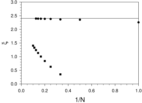
Figure 1: Comparison of convergence rates for the fully symmetric polynomial basis (filled circles) and DLCQ (filled squares). The dimensionless eigenvalue $\xi$ is plotted versus $1/N$, the reciprocal of the basis order and of the DLCQ resolution, for the case where $M^{2}=0.5\mu^{2}$. The horizontal line is at the exact value, $\xi=2.40335$.

IV Summary

We have constructed an orthonormal set of fully symmetric polynomials on a triangle that can be used as a basis for three-boson longitudinal wave functions in field theories quantized on the light front Dirac ; DLCQreview . At each order, the number of polynomials is quite small, the limitation to symmetry under the interchange of all three barycentric coordinates being a much stronger constraint than just symmetry under interchange of the two independent variables. A list of the first six polynomials is given in Eq. (16). In general, the polynomials are formed by first constructing a non-orthonormal set according to Eq. (14), and then applying an orthogonalizing procedure, such as the Gramm–Schmidt process.

As a sample application, we have considered a light-front Hamiltonian eigenvalue problem in $\phi^{4}$ theory, limited to the coupling of one-boson and three-boson Fock states. The polynomial expansion for the wave function yields rapidly converging results, particularly in comparison with a DLCQ approximation, as can be seen in Table 1 and Fig. 1.

The original motivation for these developments was to find an expansion applicable to the nonlinear equations of the light-front coupled-cluster (LFCC) method LFCC . In this method, there is no truncation of Fock space, but approximations for the wave functions for higher Fock states are determined from the wave functions of the lowest states by functions that satisfy nonlinear integral equations. In bosonic theories, these functions must have the full symmetry, and any basis used should have this symmetry. The sample application here can be interpreted as a linearization of the $\phi^{4}$ LFCC equations. Thus, we expect the new polynomial basis to be of considerable utility.

Appendix A Proof of the conjecture

Here we give a proof that any fully symmetric polynomial on a triangle can be expressed as a linear combination of products of powers of two fundamental polynomials of order two and three. We work in terms of the translated variables $u$, $v$, and $w$ defined in (5), so that the constraint of being on the triangle is $u+v+w=0$. The structure of the proof is first to characterize unconstrained polynomials on the unit cube and then to restrict these polynomials to the triangle.

Any symmetric polynomial built from mononials of order $N$ is a linear combination of polynomials $\tilde{P}_{ijk}(u,v,w)$ defined by

$$\tilde{P}_{ijk}(u,v,w)=u^{i}v^{j}w^{k}+\,\mbox{permutations},$$ (36)

with $i+j+k=N$ and $i\leq j\leq k$. Thus, the $\tilde{P}_{ijk}$ form a basis for symmetric three-variable polynomials with each term of order $N$. The size of this basis is

$$S_{N}\equiv\sum_{i=0}^{[N/2]}\sum_{j=i}^{[(N-i)/2]}1,$$ (37)

where $[x]$ means the integer part of $x$. The limits on the sums guarantee the order $i\leq j\leq k$, with $k=N-i-j$.

We can also build symmetric polynomials from linear combinations of

$$\tilde{C}_{lnm}(u,v,w)=\tilde{C}_{1}^{l}(u,v,w)\tilde{C}_{2}^{n}(u,v,w)\tilde{C}_{3}^{m}(u,v,w),$$ (38)

where

$$\tilde{C}_{1}=u+v+w,\;\;\tilde{C}_{2}=uv+uw+vw,\;\;\tilde{C}_{3}=uvw,$$ (39)

and $N=l+2n+3m$. However, is this sufficient to generate all such polynomials? The number of polynomials $\tilde{C}_{lmn}$ is

$$\Xi_{N}\equiv\sum_{m=0}^{[N/3]}\sum_{n=0}^{[(N-3m)/2]}1,$$ (40)

which counts the number of ways that the integers $l$, $n$, and $m$ can be assigned, with $l=N-2n-3m$. The substitutions $m=i$ and $n=j-i$ yield

$$\Xi_{N}=\sum_{i=0}^{[N/3]}\sum_{j=i}^{[(N-i)/2-i]+i}1=\sum_{i=0}^{[N/3]}\sum_{j=i}^{[(N-i)/2]}1.$$ (41)

Therefore, $\Xi_{N}$ is equal to $S_{N}$, and the $\tilde{C}_{lnm}$ do form an equivalent basis on the unit cube.

The projection onto the triangle $u+v+w=0$ eliminates $\tilde{C}_{1}$ and any basis polynomial $\tilde{C}_{lnm}$ with $l>0$. Thus, the basis polynomials on the triangle can be chosen as products of powers of second and third-order polynomials. The powers $n$ and $m$, respectively, include all possible integers that satisfy $N=2n+3m$. In terms of the Cartesian variables $x$ and $y$, we then have the basis set specified by (13) and (14).

References

- (1) P.A.M. Dirac, Rev. Mod. Phys. 21, 392 (1949).
- (2) For reviews of light-cone quantization, see M. Burkardt, Adv. Nucl. Phys. 23, 1 (2002); S.J. Brodsky, H.-C. Pauli, and S.S. Pinsky, Phys. Rep. 301, 299 (1998).
- (3) See, for example, G.M.-K. Hui and H. Swann, Contemporary Mathematics 218, 438 (1998).
- (4) For general discussion of multivariate polynomials, see C.F. Dunkl and Y. Xu, Orthogonal Polynomials of Several Variables, (Cambridge, New York, 2001); P.K. Suetin, Orthogonal Polynomials in Two Variables, (Gordon and Breach, Amsterdam, 1999).
- (5) H.-C. Pauli and S.J. Brodsky, Phys. Rev. D 32, 1993 (1985); 32, 2001 (1985).
- (6) S.S. Chabysheva and J.R. Hiller, Phys. Lett. B 711, 417 (2012).