“Intelligent” controllers
on cheap and small
programmable devices

Abstract

It is shown that the “intelligent” controllers which are associated to the recently introduced model-free control synthesis may be easily implemented on cheap and small programmable devices. Several successful numerical experiments are presented with a special emphasis on fault tolerant control.
Keywords— Model-free control, intelligent PID controllers, small programmable devices, estimation, identification, noise attenuation, fault tolerant control.

I Introduction

It is well know that the overwhelming majority of industrial control applications is based on PID controllers (see, e.g., [1, 17], and the references therein). Those controllers are often manufactured by numerous companies as microcontrollers on cheap and small programmable devices, like a Microchip PIC or a Freescale DSC for instance This communication demonstrates that the recent model-free control [6] and the corresponding intelligent PID controllers [6] may also be implemented on such devices,

• thanks to the low power computation cost which they require,

• although they obey to mathematical principles, which are quite different from those of “classic” PIDs.

When compared to a PID regulator, its intelligent counterpart contains one term more, which subsumes not only the unknown structure of the plant but also the unknown disturbances. This term, which is estimated online thanks to recent parameter identification techniques ([8, 9]), is also found in the linear ultra-local model which

• replaces the unknown global description of the plant,

• is continuously updated online via the same calculations,

• is of low order, which is most of the time equal to $1$.

Remark I.1

Let us emphasize moreover that the strange ubiquity of classic PIDs was mathematically explained for the first time, to the best of our knowledge, thanks to intelligent PIDs [6].

This aim is fully justified by the following facts:

• Intelligent PIDs are much easier to tune than the classic ones.

• They are robust with respect to most disturbances, including quite strong ones.

• They permit straightforward fault accommodations.

• Many successful concrete applications were already achieved in most various domains within a few years (see the numerous references in [6]).

Our paper is organized as follows. Section II summarizes some of the most important facts about model-free control and its corresponding intelligent controllers. The implementation on small programmable devices is detailed in Section III. Section IV describes some numerical experiments, with a peculiar emphasis on fault tolerant control, i.e., on an important topic in control engineering (see, e.g., [3, 16], and the references therein). Several excellent simulations are provided. Some concluding remarks may be found in Section V.

II Model-free control: Basics

II-A The ultra-local model

The unknown global description of the plant is replaced by the ultra-local model

$${y^{(\nu)}=F+\alpha u}$$ (1)

where

• the derivation order $\nu\geq 1$ is selected by the practitioner;

• $\alpha\in\mathbb{R}$ is chosen by the practitioner such that $\alpha u$ and $y^{(\nu)}$ are of the same magnitude.

Remark II.1

Note that $\nu$ has no connection with the order of the unknown system, which may be with distributed parameters, i.e., which might be best described by partial differential equations (see, e.g., [13] for hydroelectric power plants).

Remark II.2

The existing examples show that $\nu$ may always be chosen quite low, i.e., $1$ or $2$. In almost all existing concrete case-studies $\nu=1$. The only counterexample until now where $\nu=2$ is provided by magnetic bearings [4] where frictions are almost negligible.

Some comments on $F$ are in order:

• $F$ is estimated via the measure of $u$ and $y$;

• $F$ subsumes not only the unknown structure of the system but also any perturbation.

II-B Intelligent PIDs

Set $\nu=2$ in Equation (1):

$$\ddot{y}=F+\alpha u$$ (2)

Close the loop via the intelligent proportional-integral-derivative controller, or iPID,

$${u=-\frac{F-\ddot{y}^{\ast}+K_{P}e+K_{I}\int e+K_{D}\dot{e}}{\alpha}}$$ (3)

where

• $e=y-y^{\star}$ is the tracking error,

• $K_{P}$, $K_{I}$, $K_{D}$ are the usual tuning gains.

Combining Equations (2) and (3) yields

$$\ddot{e}+K_{D}\dot{e}+K_{P}e+K_{I}\int e=0$$

where $F$ does not appear anymore. The tuning of $K_{P}$, $K_{I}$, $K_{D}$ is therefore quite straightforward. This is a major benefit when compared to the tuning of “classic” PIDs (see, e.g., [1, 17], and the references therein).

Remark II.3

If $K_{I}=0$ we obtain the intelligent proportional-derivative controller, or iPD,

$${u=-\frac{F-\ddot{y}^{\ast}+K_{P}e+K_{D}\dot{e}}{\alpha}}$$

Set now $\nu=1$ in Equation (1):

$$\dot{y}=F+\alpha u$$ (4)

The loop is closed by intelligent proportional-integral controller, or iPI,

$$u=-\frac{F-\dot{y}^{\ast}+K_{P}e+K_{I}\int e}{\alpha}$$ (5)

If $K_{I}=0$, it yields an intelligent proportional controller, or iP,

$$\boxed{u=-\frac{F-\dot{y}^{\ast}+K_{P}e}{\alpha}}$$ (6)

Remark II.4

Equation (6) and the corresponding iPs are most common in practice. This is again a major simplification with respect to “classic” PIDs and PIs.

II-C Estimation of $F$

$F$ in Equation (1) is assumed to be “well” approximated by a piecewise constant function $F_{\text{est}}$. According to the algebraic parameter identification developed in [8, 9], rewrite, if $\nu=1$, Equation (4) in the operational domain (see, e.g., [23])

$$sY=\frac{\Phi}{s}+\alpha U+y(0)$$

where $\Phi$ is a constant. We get rid of the initial condition $y(0)$ by multiplying both sides on the left by $\frac{d}{ds}$:

$$Y+s\frac{dY}{ds}=-\frac{\Phi}{s^{2}}+\alpha\frac{dU}{ds}$$

Noise attenuation is achieved by multiplying both sides on the left by $s^{-2}$. It yields in the time domain the realtime estimate

$${\small F_{\text{est}}(t)=-\frac{6}{\tau^{3}}\int_{t-\tau}^{t}\left[(\tau-2\sigma)y(\sigma)+\alpha\sigma(\tau-\sigma)u(\sigma)\right]d\sigma}$$

where $\tau>0$ might be quite small. This integral may of course be replaced in practice by a classic digital filter.

III Implementation

Let us remind that implementing controllers on small programmable devices is a well established topic in engineering (see, e.g., [11, 12, 18, 20, 21, 22], and the references therein).

III-A The iP device

We first detail the implementation of the iP device, which is most of the time sufficient in practice.

III-A1 Device

The device is a microchip dsPIC33FJ128GP204 characterized by:

• Architecture: 16-bit.

• CPU speed (MIPS): 40.

• Memory type: Flash.

• Program memory (KB): 128.

We also utilize

• two inputs with a 12-bit, 500 KSPS analog-to-digital conversion,

• one 12-bit digital output coupled with an external digital-to-anolog converter.

The values of the input and output variables, which are expressed in volts, are in the range $[0,3.3]$. They can be connected however to an electronic amplifier stage. Let us add that our material is cheap: it costs less than $5$ euros.

Figure 1 displays the corresponding architecture:

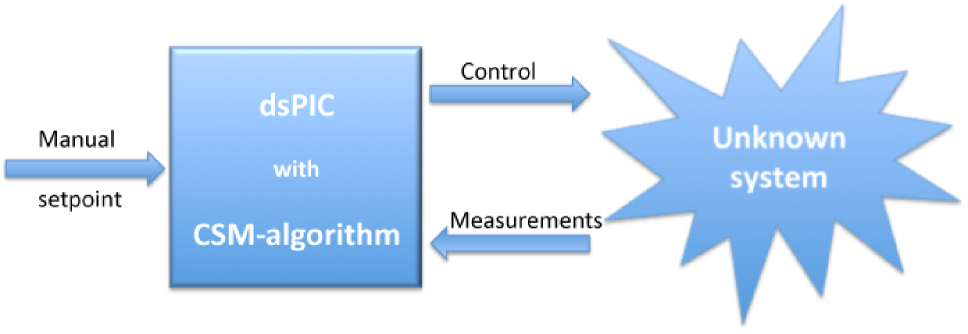
Figure 1: Control scheme

III-A2 Simple calculations

A control iteration needs:

• affectations: 19,

• conditions (if…then…else): 5,

• additions/subtractions: 14,

• multiplications/divisions: 16.

The computational power which is used is indeed very low.

III-B Some extensions

Some new calculations are of course needed for iPIs, iPIDs, and iPDs.

Remark III.1

An iPD was employed only once, for magnetic bearings [4]. Note moreover that it was not necessary until now to use iPIDs in practice!

The integrals $\int e$ appearing in iPIs and iPIDs may be dealt via the classic trapezoidal rules (see, e.g., [2]). Less than $10$ basic operations are used.

The derivative $D(t)=K_{D}\dot{e}$ in iPIDs and iPDs may be obtained via

• a backward Euler difference scheme (see, e.g., [2])

  $$D(t_{k})=K_{D}\frac{e(t_{k})-e(t_{k-1})}{t_{k}-t_{k-1}}$$

• a low-pass digital filter for reducing the noise (see, e.g., [10]).

As above for the integration, less than 10 basic operations are used.

Remark III.2

With very noisy signals, more advanced tools might be necessary for the differentiation (see [7, 15], and [14]).

IV Numerical experiments

IV-A LabVIEW

As well known, LabVIEW greatly facilitates numerical simulations in engineering and in science. LabView can be programmed in order to control a real system by the use of an input-output device (analogic and logic inputs and outputs). Simple as well as advanced regulation strategies may therefore be assessed. It may also be used for emulating/simulating the behavior of a real system (see, e.g., [19]). Emulation is achieved in our experimental platform via Labview and an input-output card (see Figure 2).

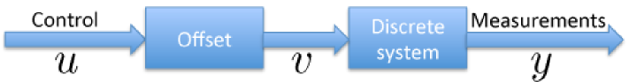
Figure 2: LabVIEW details

Note that $v$ becomes the true input control variable, where $-1.65\leq v\leq 1.65$. The non-negativity condition on $u$ (see Section III-A1) is therefore dropped. Negative values for the control variables are now possible. Figure 3 displays a full description of our devices where the dsPIC is connected to an interface from National Instrument.

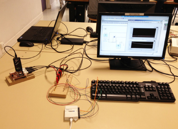
Figure 3: Our experimental setup with a dsPIC connected to an input-output card driven by LabVIEW

IV-B Two experiments

In both experiments the same iP is implemented where $\alpha=1$ and $K_{P}=1$. The control variable is obtained thanks to the dsPIC with a sample time equal to $0.1\textup{ms}$.

IV-B1 System 1

Consider the nonlinear stable system:

$$2(3\dot{v}v^{2}+v^{3})=0.5\ddot{y}+0.5\dot{y}-y$$

where $v$ is the saturated control after offset (see Figure 2 for an explanation). The tracking performances, which are presented in Figure 4, are quite good. They however deteriorate with important change points. This is due to the saturation of the control variable which is bounded.

Set

$$\bar{v}=\pi v$$

where

• $\pi=1$ corresponds to the fault-free case,

• Figure 5-(c) shows the case $0\leq\pi\nleq 1$, which corresponds to a power loss of the actuator.

Figures 5-(a) and 5-(b) display an excellent fault tolerant control even with violent faults.

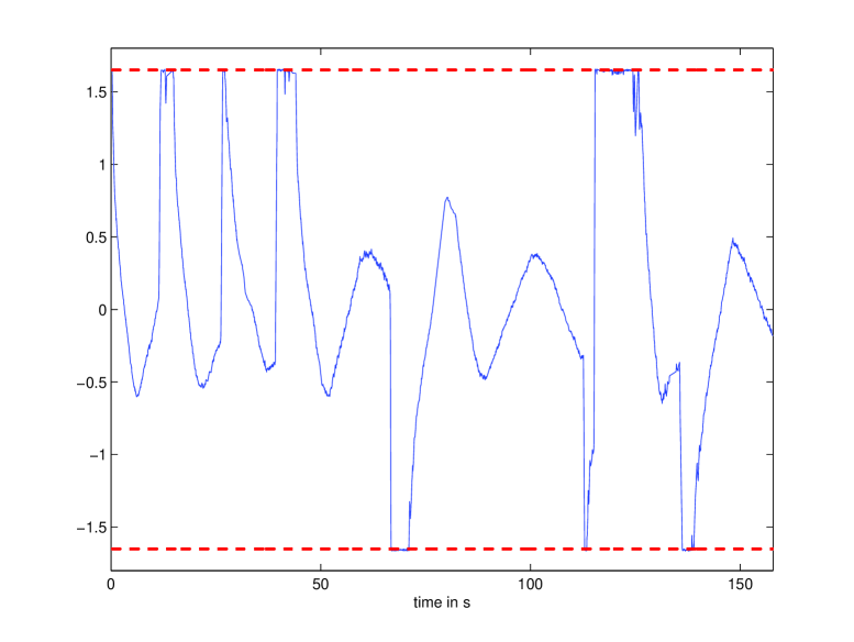
(a) Control (– blue) and control limits (- - red)

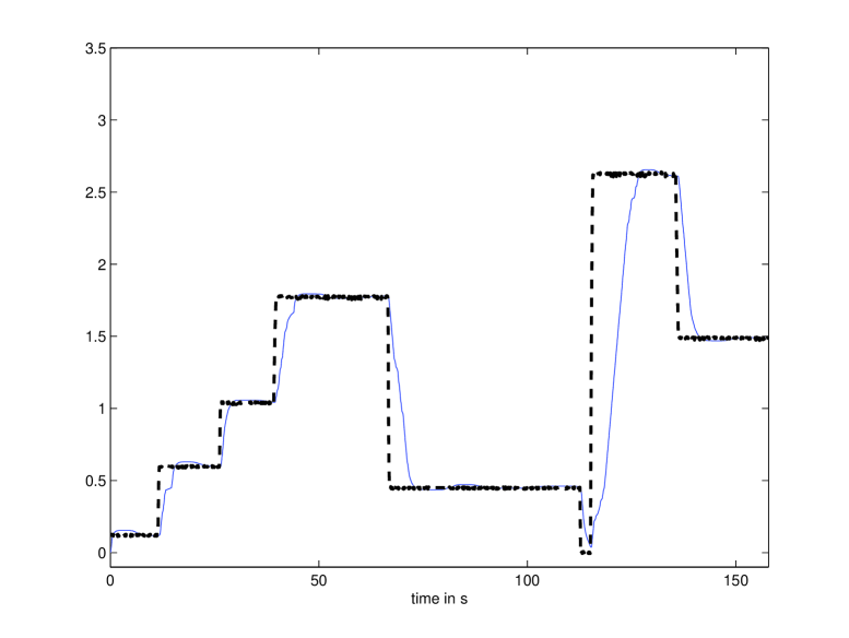
(b) Setpoint (- - black) and output (– blue)

Figure 4: Experimental results: fault-free case

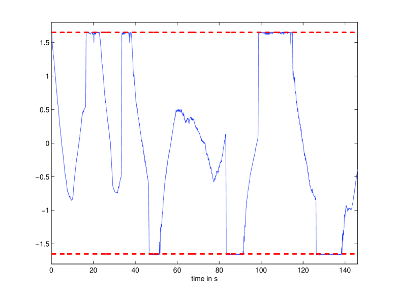
(a) Control (– blue) and control limits (- - red)

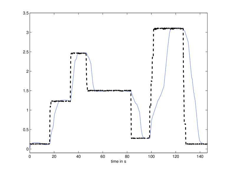
(b) Setpoint (- - black) and output (– blue)

(c) Multiplicative power loss

Figure 5: Experimental results: faulty case

IV-B2 System 2

Consider the nonlinear unstable system:

$$9\dot{v}v^{2}+v^{3}=\ddot{y}+\dot{y}+y$$

Close the loop with the same iP as above. Figure 6 displays excellent tracking and fault accommodation performances.

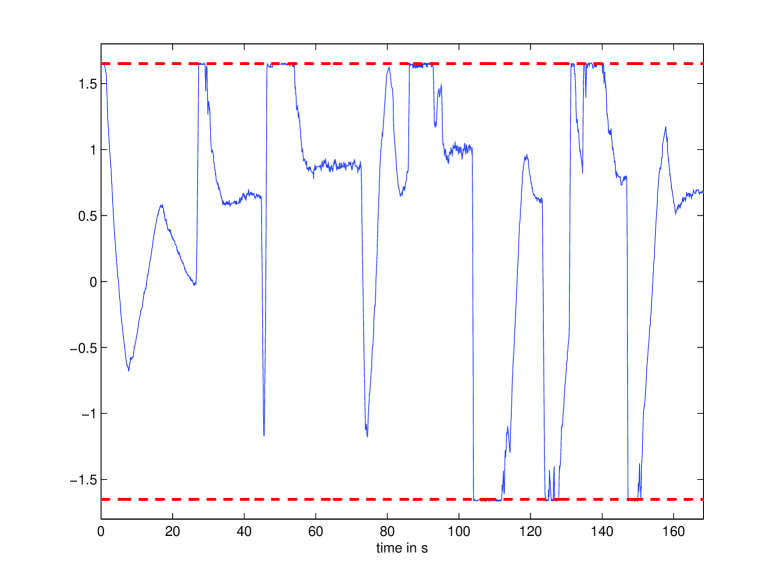
(a) Control (–,blue) and control limits (- -,red)

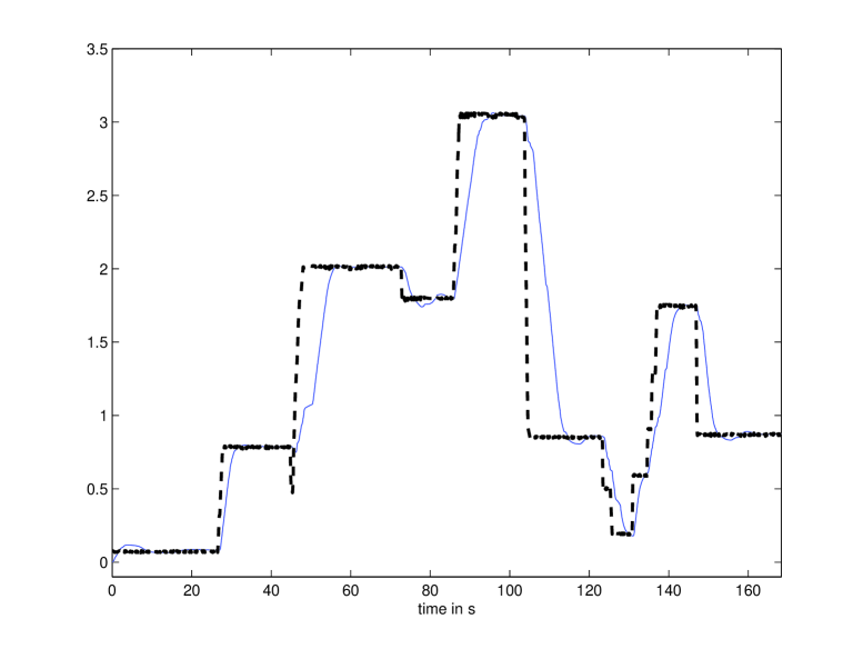
(b) Setpoint (- - black) and Output (– blue)

Figure 6: Experimental results: fault free case

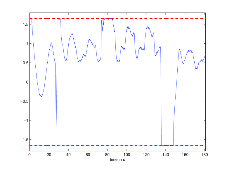
(a) Control (– blue) and control limits (- - red)

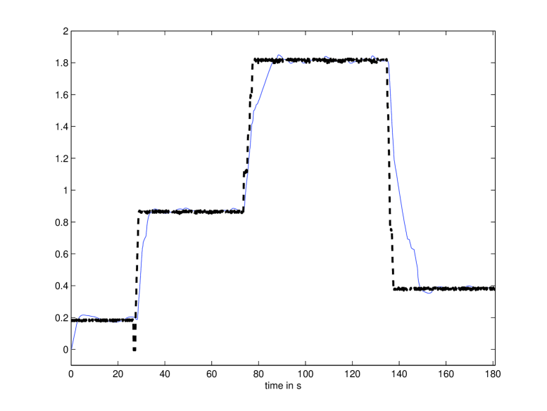
(b) Setpoint (- - black) and output (– blue)

(c) Multiplicative power loss

Figure 7: Experimental results: faulty case

V Conclusion

This communication has demonstrated that the intelligent controllers, which are associated to model-free control, may easily be implemented on cheap and small programmable devices. Future applications will show that our academic numerical experiments may be easily extended to more realistic case-studies. It should lead to great industrial opportunities for this new setting.

Acknowledgement: The authors thank the department of Génie Électrique et Informatique Industrielle, Institut Universitaire de Technologie Nancy-Brabois, Université de Lorraine, for its most friendly help and its loan of some essential devices.

References

- [1] K.J. Åström, T. Hägglund, Advanced PID Control, Instrument Soc. Amer., 2006.
- [2] K.E. Atkinson, An Introduction to Numerical Analysis (2nd ed.), Wiley, 1989.
- [3] M. Blanke, M. Kinnaert, J. Lunze, M. Staroswiecki, Diagnosis and Fault-Tolerant Control, Springer, 2003.
-
[4]
J. De Miras, S. Riachy, M. Fliess, C. Join, S. Bonnet,
Vers une commande sans modèle d’un palier magnétique,
7e Conf. Internat. Francoph. Automatique, Grenoble, 2012.
Available at
http://hal.archives-ouvertes.fr/hal-00682762/en/ - [5] M. Fliess, Analyse non standard du bruit, C.R. Acad. Sci. Paris Ser. I, vol. 342, pp. 797–802, 2006.
-
[6]
M. Fliess, C. Join,
Model-free control,
Int. J. Control, 2013, DOI: 10.1080/00207179.2013.810345. Preprint available at
http://hal.archives-ouvertes.fr/hal-00828135/en/ -
[7]
M. Fliess, C. Join, H. Sira-Ramírez,
Non-linear estimation is easy,
Int. J. Model. Identif. Control, vol. 4, pp. 12–27, 2008. Preprint available at
http://hal.archives-ouvertes.fr/inria-00158855/en/ - [8] M. Fliess, H Sira-Ramírez, An algebraic framework for linear identification, ESAIM Control Optimiz. Calc. Variat., 9: 151–168, 2003.
- [9] M. Fliess, H. Sira-Ramírez, Closed-loop parametric identification for continuous-time linear systems via new algebraic techniques, in eds. H. Garnier and L. Wang, Identification of Continuous-time Models from Sampled Data, Springer, pp. 362–391, 2008.
- [10] G.F. Franklin, M.L. Workman, D. Powell, Digital Control of Dynamic Systems (3rd ed.), Addison-Wesley, 1997
- [11] A.P. Godse, D.A. Godse, Microprocessors and Microcontrollers (6th revised ed.), Technical Editions Pune, 2009.
- [12] D. Ibrahim, Microcontroller Based Applied Digital Control, Wiley, 2006.
-
[13]
C. Join, G. Robert, M. Fliess,
Vers une commande sans modèle pour aménagements hydroélectriques en cascade,
6e Conf. Internat. Francoph. Automat., Nancy, 2010.
Available at
http://hal.archives-ouvertes.fr/inria-00460912/en/ - [14] D.Y. Liu, O. Gibaru, W. Perruquetti, Error analysis of Jacobi derivative estimators for noisy signals, Numer. Algor., 58, 53–83, 2011.
- [15] M. Mboup, C. Join, M. Fliess, Numerical differentiation with annihilators in noisy environment, Numer. Algor., 50, 439–467, 2009.
- [16] H. Noura, D. Theilliol, J.-C. Ponsart, A. Chamseddine, Fault-tolerant Control Systems - Design and Practical Applications, Springer, 2009.
- [17] A. O’Dwyer, Handbook of PI and PID Controller Tuning Rules (3rd ed.), Imperial College Press, 2009.
- [18] J.S. Parab, V.G. Shelake, R.K. Kamat, G.M. Naik, Practical Aspects of Embedded System Design Using Microcontrollers, Springer, 2008
- [19] A. St. Leger, A. Deese, J. Yakaski, C. Nwankpa, Controllable analog emulator for power system analysis, Int. J. Electrical Power Energy Syst., 33, 1675–1685, 2011.
- [20] C. Tavernier, Applications des microcontrôleurs PIC (4e éd.), Dunod, 2011.
- [21] J.W. Valvano, Embedded Microcomputer Systems – Real Time Interfacing (3rd ed.), Cengage Learning, 2011.
- [22] T. Wilmshurst, Designing Embedded Systems with PIC Microcontrollers: Principles and Applications, Elsevier, 2007.
- [23] K. Yosida, Operational Calculus (translated from the Japanese), Springer, 1984.