FullSWOF_Paral: Comparison of two parallelization strategies (MPI and SKELGIS)
on a software designed for hydrology applications

Abstract

In this paper, we perform a comparison of two approaches for the parallelization of an existing, free software, FullSWOF_2D (http://www.univ-orleans.fr/mapmo/soft/FullSWOF/ that solves shallow water equations for applications in hydrology) based on a domain decomposition strategy. The first approach is based on the classical MPI library while the second approach uses Parallel Algorithmic Skeletons and more precisely a library named SkelGIS (Skeletons for Geographical Information Systems). The first results presented in this article show that the two approaches are similar in terms of performance and scalability. The two implementation strategies are however very different and we discuss the advantages of each one.

1 Problematics

We are interested in overland flow simulations. For this kind of flow simulation, several methods are used from empirical models to physically based models. Two physical models are often used to model overland flow kinematic (KW) and diffusive wave (DW) equations [1], [2]. But following [3], [4], [5], we choose to use the shallow water (Saint-Venant [6]) physical model. Indeed KW and DW models may give poor results in terms of water heights and velocities in case of mixed subcritical and supercritical flows. Despite the computational cost, shallow water model is mandatory. MacCormack scheme is widely used to solve shallow water (SW) equations [3], [4], [5]. But it neither guarantees the positivity of water depths at the wet/dry transitions, nor preserves steady states (not well-balanced [7]) as noticed in [8]. In industrial codes (ISIS, Canoe, HEC-RAS, MIKE11, …), SW equations are often solved under non-conservative form [9, 10, 2] with either Preissmann scheme or Abbott-Ionescu scheme. Thus transcritical flows and hydraulic jumps are not solved properly. In order to cope with all these problems, we have developed FullSWOF_2D (Full Shallow Water equations for Overland Flow) an object-oriented C++ code (free software and GPL-compatible license CeCILL-V2) in the framework of the multidisciplinary project METHODE (see [11] and http://www.univ-orleans.fr/mapmo/methode/). The source code is available at http://www.univ-orleans.fr/mapmo/soft/FullSWOF/. This software is based on the physical model of shallow water equations (Saint-Venant system [6]) for the water runoff, coupled with Green-Ampt’s infiltration model [12]. The set of shallow water equations is solved thanks to a well-balanced finite volume method. This enables to catch and to preserve steady states such as puddles and lake at rest. Moreover the method preserves the positivity of the water height. Validations of FullSWOF_2D have already been performed on analytical benchmarks (SWASHES [13]), on experimental data and on real events at small scales (parcels [14, 11]). We now aim at simulating at bigger scales such as watershed, river valley or at small scales with fine details. Thus the computing time becomes bigger and the code needs to be parallelized. We want to compare two approaches: the first one is a ”classical” approach based on a master-slave architecture using MPI and the second one uses skeletal algorithms (SkelGIS, Skeletons for Geographical Information Systems, which is under development by Hélène Coullon, a CIFRE PhD student with Géo-Hyd company). These approaches will be compared both in terms of performance and scalability and the advantages of each choice will be briefly discussed.

2 Physical model

2.1 General settings

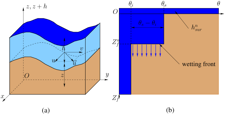
Figure 1: Variables of (a) 2D shallow water equations (SW2D) and (b) Green-Ampt infiltration model.

As in [4, 5], we model overland flow thanks to the 2D shallow water equations (SW2D). Shallow water equations (or Saint-Venant system) have been proposed by Adhémar Barré de Saint-Venant in 1871 in order to model flows in channels [6] in one dimension in space. Nowadays, they are used to model flows in various contexts, such as: overland flow [4, 15], rivers [16, 17], flooding [18, 19], dam breaks [20, 21], nearshore [22, 23], tsunami [24, 25, 26]. These equations consist in a nonlinear system of partial differential equations (PDE-s), more precisely conservation laws describing the evolution of the height ($h(t,x,y)$ [L]) and the horizontal components of the vertically averaged velocity of the fluid ($\vec{u}(t,x,y)=(u(t,x,y),v(t,x,y))^{t}$ [L/T]) as illustrated on figure 1-a. This complete set of conservation laws writes

$$\left\{\begin{array}[]{l}\partial_{t}h+\partial_{x}(hu)+\partial_{y}(hv)=R-I\\ \partial_{t}(hu)+\partial_{x}\left(hu^{2}+gh^{2}/2\right)+\partial_{y}\left(huv\right)=gh\left({S_{0}}_{x}-{S_{f}}_{x}\right)\\ \partial_{t}(hv)+\partial_{x}\left(huv\right)+\partial_{y}\left(hv^{2}+gh^{2}/2\right)=gh\left({S_{0}}_{y}-{S_{f}}_{y}\right)\end{array}\right.$$ (1)

where

• $g=9.81\,\text{m}/\text{s}^{2}$ is the gravity constant;

• $z(x,y)$ is the topography [L] and we denote by ${S_{0}}_{x}=-\partial_{x}z(x,y)$ (resp. ${S_{0}}_{y}=-\partial_{y}z(x,y)$) the opposite of the slope in the $x$ (resp. $y$) direction. Erosion is not considered here, so the topography is a fixed function of space. Equations might be added to SW2D model to take erosion effect into account. We get systems such as Saint-Venant Exner and Hairsine & Rose models (for more details see [27]);

• $R(t,x,y)\geq 0$ [L/T] is the rain intensity;

• $I(t,x,y)$ [L/T] is the infiltration rate. It is given by another model (such as Green-Ampt [12], Richards [28], …);

• and $\vec{S}_{f}=\left({S_{f}}_{x},{S_{f}}_{y}\right)$ is the friction force vector. It may take several forms, depending on soil and flow properties. In hydrological and hydraulics models, two families of friction laws are mainly encountered. They are based on empirical considerations. On one hand, we have the family of Manning-Strickler’s friction laws

  $$\vec{S}_{f}=C_{f}\dfrac{\sqrt{u^{2}+v^{2}}}{h^{4/3}}\vec{u},$$

  $C_{f}=n^{2}$ (resp. $C_{f}=1/K^{2}$), where $n$ (resp. $K$) is the Manning’s coefficient [L^-1/3T] (resp. Strickler’s coefficient [L^-1/3T]). On the other hand, we have the law of Darcy-Weisbach’s and Chézy’s family

  $$\vec{S}_{f}=C_{f}\dfrac{\sqrt{u^{2}+v^{2}}}{h}\vec{u},$$

  $C_{f}=f/(8g)$ (resp. $C_{f}=1/C^{2}$), where $f$ (resp. $C$) is the dimensionless Darcy-Weisbach’s coefficient (resp. Chézy’s coefficient [L^1/2/T]). The friction may depend on the space variable, especially on large parcels and watersheds. Values of friction coefficients depend on the considered type of soil and are tabulated in references such as [29].

System (1) will be solved on a Cartesian grid thanks to a method of lines. Thus the numerical strategy consists in choosing a numerical method adapted to the properties of the shallow water system in 1D (SW1D). Then the generalization to SW2D is straightforward. So in next sections, we will consider SW1D system.

2.2 Hyperbolicity

As previously argumented, we place ourselves in the one-dimensional case. SW1D system writes

$$\left\{\begin{array}[]{l}\partial_{t}h+\partial_{x}(hu)=R-I\\ \partial_{t}(hu)+\partial_{x}\left(hu^{2}+gh^{2}/2\right)=gh\left({S_{0}}-{S_{f}}\right)\end{array}\right..$$ (2)

The left-hand side of system (2) is a transport operator, corresponding to the flow of an ideal fluid in a flat channel, without friction, rain or infiltration. This corresponds to the model introduced by Saint-Venant [6] which contains several flow properties. To emphasize these properties, we rewrite the one-dimensional homogeneous system under vectors form

$$\partial_{t}U+\partial_{x}F(U)=0,\;\text{where}\;U=\left(\begin{array}[]{c}h\\ hu\end{array}\right)=\left(\begin{array}[]{c}h\\ q\end{array}\right),\;F(U)=\left(\begin{array}[]{c}hu\\ hu^{2}+gh^{2}/2\end{array}\right),$$ (3)

with $F(U)$ the flux of the equation and $q(t,x)$ [L²/T] the discharge by unit of width. The transport property of system (3) is clearer under the following nonconservative forms

$$\partial_{t}U+A(U)\partial_{x}U=0,\;A(U)=F^{\prime}(U)=\left(\begin{array}[]{cc}0&1\\ gh-u^{2}&2u\end{array}\right),$$

where the Jacobian matrix $A(U)=F^{\prime}(U)$ is the matrix of transport coefficients. When $h>0$, matrix $A(U)$ is diagonalizable and its eigenvalues are

$$\lambda_{1}(U)=u-\sqrt{gh}<u+\sqrt{gh}=\lambda_{2}(U).$$ (4)

System (3) is strictly hyperbolic. The eigenvalues are the velocities of the surface waves and thus are basic characteristics of flows. Notice that these eigenvalues collapse in one when $h=0\,\text{m}$ (for dry zones). In that case, system (3) is no longer hyperbolic which is difficult to deal with both from theoretical and numerical levels. Getting a numerical scheme that preserves the water height positivity is a necessity.

Eigenvalues (4) of system (3) allow to make a classification of flows, based on the relative values of the velocities of the waves $c=\sqrt{gh}$ and of the fluid $u$. Indeed if $|u|<\sqrt{gh}$, the characteristic velocities have opposite signs and flow informations propagate both upward and downward. The flow is said to be subcritical or fluvial. When $|u|>\sqrt{gh}$, the flow is supercritical or torrential and all informations propagate downstream. This has to be taken into account both for the numerical methods (upwinding) and the boundary conditions.

Numerically, boundary conditions are expected to provide numerical fluxes at the boundaries of domain. These are required in order to update $(h,q)$ on the extreme cells to the next time level. The boundary conditions may result in direct prescription of the numerical fluxes at the boundaries. Alternatively, we may prescribe the values of $(h,q)$ on the ghost cells. In this way, the Riemann problems at the boundaries are solved and the corresponding fluxes are computed as done for the interior cells. The values of $(h,q)$ on ghost cells can be computed in function of flow regime thanks to the Riemann invariants (which remain constant along the corresponding characteristic line). For subcritical flow, the characteristic $dx/dt=u-c$ leaves the domain while the characteristic $dx/dt=u+c$ enters the domain. Thus for numerical simulations, we impose one variable ($h$ or $q$) for fluvial inflow/ouflow. In contrary, both variable must be prescribed in case of supercritical inflow whereas free boundary conditions are considered for supercritical outflow. We refer to [30] for more details.

With the presence of the source terms, an other main property has to be considered: the occurrence of steady states or stationary solutions. These particular flows are studied in next section.

2.3 Steady flows

Steady states solutions correspond to stationary flows, i.e. solutions that satisfy

$$\partial_{t}h=\partial_{t}u=\partial_{t}q=0,$$

system (2) reduces in

$$\left\{\begin{array}[]{l}\partial_{x}(hu)=R-I\\ \partial_{x}\left(hu^{2}+gh^{2}/2\right)=gh\left({S_{0}}-{S_{f}}\right)\end{array}\right..$$ (5)

To our knowledge there is no scheme designed to preserve these stationary flows. If we consider no rain $R=0$, no infiltration $I=0$ and no friction $S_{f}=0$, system (5) reduces in

$$\left\{\begin{array}[]{l}\partial_{x}(hu)=0\\ \partial_{x}\left(hu^{2}+gh^{2}/2\right)=-gh\partial_{x}z\end{array}\right..$$

We recover Bernoulli’s law

$$\left\{\begin{array}[]{l}hu=q=Cst\\ \dfrac{q^{2}}{2gh^{2}}+h+z=Cst\end{array}\right.,$$ (6)

where $h+z$ is the free surface water level.

Several schemes have been designed to preserve steady states (6). In general, these methods are costly in term of implementation and computation because, for example, they lead to solve a third order polynomial and the appropriate root must be selected depending on the type of flow (see e.g. [31]). Moreover, the preserving of steady states (6) becomes more complicated when we require also the positivity preserving of water depths at numerical level. As the last property is a compulsory property for the applications we are interested in (overland flow simulations), we limit ourselves to numerical schemes that preserve the particular steady state corresponding to equilibrium of lake at rest

$$u=q=0\;\text{and}\;h+z=Cst.$$

In that case, we have hydrostatic balance between the hydrostatic pressure and the gravitational acceleration down the inclined bottom $z$.

In 1994, Bermúdez and Vázquez [32] are the first to identify the difficulty to preserve this steady state. Schemes preserving this equilibrium have the Conservation property or C-property (introduced in [32]). They obtained such a numerical method by modifying the Roe scheme. The topography source term is upwinded thanks to a projection on the eigenvalues of Jacobian matrix of the flux. Since [7], schemes which preserve exactly at least the hydrostatic equilibrium at a discrete level are called well-balanced schemes. We can find a lot of well-balanced schemes for SW1D in the literature [32, 33, 7, 34, 35, 36, 37, 38, 39, 40, 41, 42].

In case of rainfall overland flows, we have the occurrence of wet/dry transitions and small water heights. To simulate that kind of events, we need a robust and positive well-balanced scheme. Thus we have chosen a finite volume scheme based on the hydrostatic reconstruction (introduced in [38] and [43]), that we will detail in next section.

3 Numerical method

As argued in the previous section, the numerical method will be presented in one dimension (extension to 2D being straightforward on Cartesian grids thanks to the method of lines).

3.1 Convective step

A finite volume discretization of SW1D, (2), writes

$$U_{i}^{*}=U_{i}^{n}-\dfrac{\Delta t}{\Delta x}\left[F_{i+1/2L}^{n}-F_{i-1/2R}^{n}-Fc_{i}^{n}\right]$$ (7)

with $\Delta x$ (resp. $\Delta t$) the space (resp. time) step and

$$\begin{array}[]{l}F_{i+1/2L}^{n}=F_{i+1/2}^{n}+S_{i+1/2L}^{n}\\ F_{i-1/2R}^{n}=F_{i-1/2}^{n}+S_{i-1/2R}^{n}\end{array},$$

the left and right modifications of the numerical flux $\cal F$ for the homogeneous problem (see section 3.3)

$$F_{i+1/2}^{n}={\cal F}\left(U_{i+1/2L}^{n},U_{i+1/2R}^{n}\right).$$

The values $U_{i+1/2L}$ and $U_{i+1/2R}$ are obtained thanks to two consecutive reconstructions. Firstly a MUSCL reconstruction [44, 43, 11] is performed on $u$, $h$ and $h+z$ in order to get a second order scheme in space (see section 3.4). This gives us the reconstructed values $\left(U_{-},z_{-}\right)$ and $\left(U_{+},z_{+}\right)$. Secondly, we apply the hydrostatic reconstruction [38, 43] on the water height which allows us to get a positive preserving well-balanced scheme

$$\left\{\begin{array}[]{l}h_{i+1/2L}=\max\left(h_{i+1/2-}+z_{i+1/2-}-\max\left(z_{i+1/2-},z_{i+1/2+}\right),0\right)\\ U_{i+1/2L}=\left(h_{i+1/2L},h_{i+1/2L}u_{i+1/2-}\right)^{t}\\ h_{i+1/2R}=\max\left(h_{i+1/2+}+z_{i+1/2+}-\max\left(z_{i+1/2-},z_{i+1/2+}\right),0\right)\\ U_{i+1/2R}=\left(h_{i+1/2R},h_{i+1/2R}u_{i+1/2+}\right)^{t}\end{array}\right..$$

We introduce

$$S_{i+1/2L}^{n}=\left(\begin{array}[]{c}0\\ g\left(h_{i+1/2-}^{2}-h_{i+1/2L}^{2}\right)/2\end{array}\right),\;S_{i-1/2R}^{n}=\left(\begin{array}[]{c}0\\ g\left(h_{i-1/2+}^{2}-h_{i-1/2R}^{2}\right)/2\end{array}\right)$$

and a centered source term is added to preserve consistency and well-balancing [38, 43]

$$Fc_{i}^{n}=\left(\begin{array}[]{c}0\\ -g\dfrac{h_{i-1/2+}+h_{i+1/2-}}{2}\left(z_{i+1/2-}-z_{i-1/2+}\right)\end{array}\right).$$

We have to insist on the positivity and the robustness of this method. The rain source term is treated explicitly and the infiltration rate is obtained thanks to the Green-Ampt model [12] (see section 3.5).

3.2 Friction treatment

In this step, the friction term is taken into account with the following system

$$\partial_{t}U=\left(\begin{array}[]{c}0\\ -ghS_{f}\end{array}\right).$$

This system is solved thanks to a semi-implicit method (as in [30, 5]), which writes for the Darcy-Weisbach’s law

$$h^{n+1}=h^{*}\;\text{and}\;q^{n+1}=\dfrac{q^{*}}{1+\Delta t\dfrac{f}{8}\dfrac{|q^{n}|}{h^{n}h^{n+1}}},$$

where $h^{*}$, $q^{*}$ and $u^{*}$ are the variables from the convective step. This method allows to preserve stability (under a classical CFL condition) and steady states at rest. Finally, these two steps are combined in a second order TVD Runge Kutta method which is the Heun’s predictor-corrector method [45]. It writes

$$\begin{array}[]{c}U^{*}=U^{n}+\Delta t\Phi\left(U^{n}\right)\\ U^{**}=U^{*}+\Delta t\Phi\left(U^{*}\right)\\ U^{n+1}=\dfrac{U^{n}+U^{**}}{2}\end{array}$$

where $\Phi$ is the right part of (7).

3.3 Numerical flux

About the homogeneous flux ${\cal F}\left(U_{i+1/2L}^{n},U_{i+1/2R}^{n}\right)$, we can use any consistent numerical flux, for example the one of Godunov, Rusanov, HLL, Roe or the one obtained by the kinetic or the relaxation methods. In this work, we adopted the Harten Lax van Leer (HLL) flux [46, 43, 11] which is known to be a simple and efficient solver for both accuracy and implementation aspects (see [11])

$${\cal F}\left(U_{L},U_{R}\right)=\left\{\begin{array}[]{ll}F(U_{L})&\text{if}\;0\leq c_{1}\\ \dfrac{c_{2}F(U_{L})-c_{1}F(U_{R})}{c_{2}-c_{1}}+\dfrac{c_{1}c_{2}}{c_{2}-c_{1}}\left(U_{R}-U_{L}\right)&\text{if}\;c_{1}<0<c_{2}\\ F(U_{R})&\text{if}\;c_{2}\leq 0\end{array}\right.,$$

with two parameters $c_{1}<c_{2}$ which are the approximations of slowest and fastest wave speeds respectively. We refer to [47] for further discussion on the wave speed estimates. In this paper, we use

$$c_{1}={\inf\limits_{U=U_{L},U_{R}}}({\inf\limits_{j\in\{1,2\}}}\lambda_{j}(U))\;\text{and}\;c_{2}={\sup\limits_{U=U_{L},U_{R}}}({\sup\limits_{j\in\{1,2\}}}\lambda_{j}(U)),$$

where $\lambda_{1}(U)=u-\sqrt{gh}$ and $\lambda_{2}(U)=u+\sqrt{gh}$ are the eigenvalues of SW1D. In practice, we use a CFL condition $n_{CFL}=0.5$ at second order and $n_{CFL}=1$ at first order, with

$$\Delta t\leq n_{CFL}\dfrac{\Delta x}{\max\limits_{i\in\{1,...,J\}}\left(|u_{i}|+\sqrt{gh_{i}}\right)},$$ (8)

where $J$ is the number of space cells. At second order, variables $(h_{i},u_{i})$ in (8) are replaced by the reconstructed values $(h_{i+1/2-},u_{i+1/2-})$ and $(h_{i+1/2+},u_{i+1/2+})$ (detailed in next section).

3.4 MUSCL-reconstruction

We define the MUSCL reconstruction of a scalar function $s\in\mathbb{R}$ (Monotonic Upwind Scheme for Conservation Law, see [44]) by

$$s_{i-1/2+}=s_{i}-\dfrac{\Delta x}{2}Ds_{i}\;\text{and}\;s_{i+1/2-}=s_{i}+\dfrac{\Delta x}{2}Ds_{i}$$ (9)

with the operator

$$Ds_{i}=\text{minmod}\left(\dfrac{s_{i}-s_{i-1}}{\Delta x},\dfrac{s_{i+1}-s_{i}}{\Delta x}\right)$$ (10)

and the minmod limiter

$$\text{minmod}(x,y)=\left\{\begin{array}[]{ll}\min(x,y)&\text{if}\;x,y\geq 0\\ \max(x,y)&\text{if}\;x,y\leq 0\\ 0&\text{else}\end{array}\right.$$ (11)

As mentioned previously, the MUSCL reconstruction is performed on $u$, $h$ and $h+z$, then we deduce the reconstruction of $z$. In order to keep the discharge conservation, the reconstruction of the velocity has to be modified as what follows [43]

$$u_{i-1/2+}=u_{i}-\dfrac{h_{i+1/2-}}{h_{i}}\dfrac{\Delta x}{2}Du_{i}\quad\text{and}\quad u_{i+1/2-}=u_{i}+\dfrac{h_{i-1/2+}}{h_{i}}\dfrac{\Delta x}{2}Du_{i}.$$

Thus, we recover the following conservation properties

$$\dfrac{h_{i-1/2+}+h_{i+1/2-}}{2}=h_{i}\quad\text{and}\quad\dfrac{h_{i-1/2+}u_{i-1/2+}+h_{i+1/2-}u_{i+1/2-}}{2}=h_{i}u_{i}.$$

3.5 Green-Ampt infiltration model

Infiltration is computed at each cell by using a modified Green-Ampt model [4]. The soil water movement is assumed to be in the form of an advancing front (located at $Z_{f}^{n}$ [m]) that separates a zone still at the initial soil moisture $\theta_{i}$ from a saturated zone with soil moisture $\theta_{s}$ (as illustrated on figure 1-b. At time $t=t_{n}$, infiltration capacity, $I_{C}^{n}$ [m/s], is calculated thanks to

$$I_{C}^{n}=K_{s}\left(A+\dfrac{h_{f}-h_{over}^{n}}{Z_{f}^{n}}\right)\quad\text{where}\quad Z_{f}^{n}=\dfrac{V_{inf}^{n}}{\theta_{s}-\theta_{i}},$$

where $h_{f}$ is the wetting front capillary pressure head, $K_{s}$ the hydraulic conductivity at saturation, $h_{over}^{n}$ the overland flow water height (obtained from the SW2D) and $V_{inf}^{n}$ the infiltrated water volume. Thus we have the infiltration rate (necessary to couple SW2D with Green-Ampt model)

$$I^{n}=\dfrac{\min(h_{over}^{n},\Delta t.I_{C}^{n})}{\Delta t},$$

and the infiltrated volume

$$V_{inf}^{n+1}=V_{inf}^{n}+\Delta t.I^{n},$$

where $\Delta t$ is the time step fixed by the CFL stability condition (see section 3.3).

4 FullSWOF_2D

4.1 The software

The name FullSWOF_2D stands for “Full Shallow Water equations for Overland Flow in two dimensions of space”. It is a C++ code (free open source software under the GPL-compatible license CeCILL-V2. Sources can be downloaded from http://www.univ-orleans.fr/mapmo/soft/FullSWOF/) developed in the context of the project ANR METHODE (see [11] and http://www.univ-orleans.fr/mapmo/methode/). FullSWOF_2D is based on a finite volume method (described in section 3) on a structured mesh in two space dimensions. Structured grids have been chosen because on the one hand digital topographic maps are often provided on such meshes, and, on the other hand, it allows to develop numerical schemes in one space dimension (implemented in FullSWOF_1D), extension to 2D being straightforward. As argued previously, finite volume scheme ensures by construction the conservation of the water mass, and is coupled with the hydrostatic reconstruction [38, 43] to deal with the topography source term. It preserves water height positivity and it is well-balanced (i.e. it preserves at least hydrostatic equilibrium: lakes and puddles). Several numerical fluxes (Rusanov, HLL, kinetic and VFRoe-ncv flux) and second order reconstructions (MUSCL, ENO and modified ENO reconstruction) are implemented. Currently, we recommend, based on [11], to use the second order scheme with MUSCL reconstruction [44] and HLL flux [46] detailed in section 3. FullSWOF_2D is designed in order to ease implementation of new numerical methods. FullSWOF_2D has already been validated on analytical solutions integrated in SWASHES (Shallow Water Analytic Solutions for Hydraulic and Environmental Studies: a free library of analytical solutions [13]) and on real events simulation at small scales [11, 14] (on parcels). In next section, FullSWOF_2D is validated at a bigger scale on the Malpasset test case.

4.2 Validation: Malpasset case

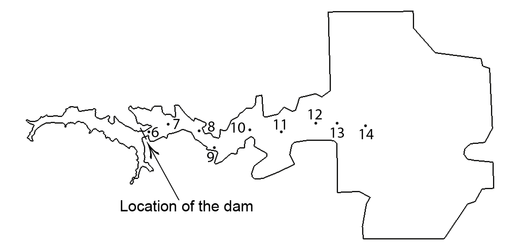
Figure 2: Position of the different gauges and location of the dam.

Malpasset dam break is a real life application. It occured (because of heavy rains) on December 2 1959 in the Var Department in southeastern France, causing 433 casualties. This dramatic event is very often mentioned in studies dealing with dam breaks and associated risks (see among others [48, 49, 50, 51, 52, 53, 54]). Because of its varying topography and complex geometry, it is widely used as a benchmark test for numerical methods and hydraulics software [55, 56, 57, 58, 39, 59, 60]. Moreover, this problem allows to test the ability of the scheme to treat the still water (at the level of the sea downstream, before the wave reaches it) and the wet-dry interfaces.

The dimensions of the domain are $dim_{x}=17273.9\;\text{m}$ along x-axis with 1000 meshes and $dim_{y}=8381.3\;\text{m}$ along y-axis with 486 meshes, the total time of simulation is $2500\;\text{s}$ and we consider the Manning law with $n=0.033$ as advised in the literature [56].

The dam is considered as a straight line (see figure 2), the water level inside the reservoir is set to 100 m above sea level and the computational domain downstream the dam is considered as dry bed. Indeed, the initial discharge in the river before dam failure can be neglected because of the huge amount of flow caused by the dam failure.

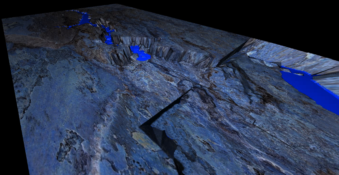
Figure 3: Propagation of the Malpasset dam break for different time 0 s and 500 s.

We run the simulation using FullSWOF_Paral over 16 processors and we get the results in Figures 3 and 4. In 1964, a physical model wih a scale of 1:400 was built by Laboratoire National d’Hydraulique to study the dam-break flow. The maximum water level and flood wave arrival time were recorded at 9 points in the physical model (named from 6 to 14). This physical model has been used to calibrate/validate Telemac_2D software [55, 56, 61] and these results are used here to validate FullSWOF_2D at “big” scale. We can see on figure 5 that the results are very closed to those obtained with Telemac. On figures 3 and 4 is represented the propagation of the wave due to the dam break (a video can be visualized on http://www.youtube.com/user/FullSWOF) and on figure 6, the propagation of the water height at the gauges during time (this will be used in future work). These results show the efficiency of FullSWOF but at that scale, details such as houses and roads are not represented. So in case of prevention, the use of these results might be limited. It might be useful to have more details. So the mesh would be finer, in that case the code needs to be parallelized.

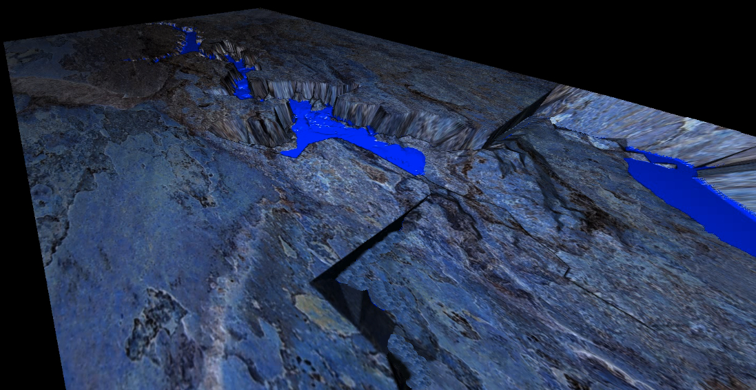
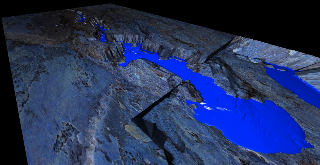
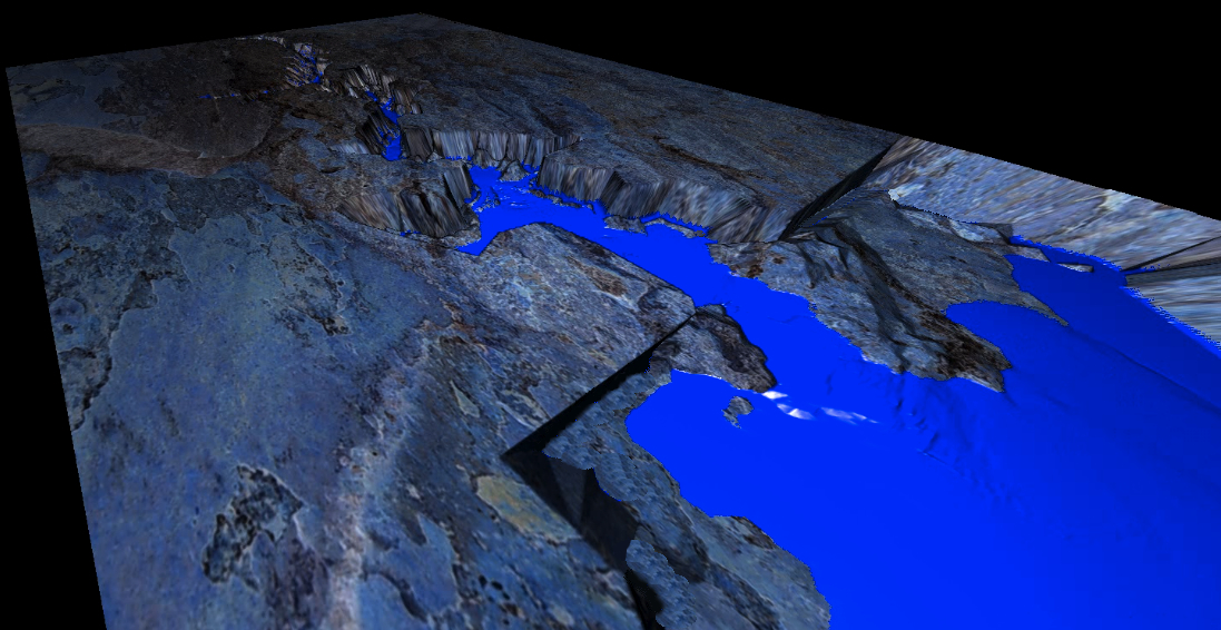
Figure 4: Propagation of the Malpasset dam break for different time 1000s, 2000 s and 2500 s.

Figure 5: Comparison of the maximum height of the water level in all gauges between FullSWOF_2D and Telemac_2D.

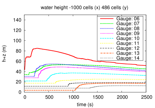
Figure 6: Propagation of the water height for different gauges during time.

5 SkelGIS

5.1 Purpose

Parallelism [62] is an intricate domain of computing science. Indeed, in addition to good sequential and parallel programming skills, it requires also a strong knowledge on processors, memory and network use to be able to write optimal programs on modern parallel computers. Writing a parallel program is long and complex, and implementing optimizations to get very good performances is even more difficult. As a consequence, giving the opportunity to non-specialists and even to non-computer scientists to use parallelism is a major research area for a long time. Indeed, in lots of domains high performance computing has become a crucial point.

A wide range of solutions exists to give access to parallelism to non-specialists. Most of them require the collaboration of experts in parallelism with the scientists of the targeted domain since classical parallel libraries are too technical. A good alternative is to propose libraries that clearly separate the parallelism side from the user side. Those tools provide some parallel patterns that hide the technical details of parallelism and are optimized for a class of problems. Such libraries give a restricted access to parallelism but greatly simplify the program development. The difficulty is to find the good balance between the level of abstraction, to hide the parallelism, and the performance of the program.

SkelGIS library is presented in this part and takes place in the latter category of libraries. SkelGIS is an algorithmic skeleton library and has been used to parallelize FullSWOF_2D.

5.2 Algorithmic skeletons

Algorithmic parallel skeletons were introduced in 1988 by Muray Cole [63]. The domain of algorithmic skeletons aims at providing generalist patterns of parallelization to the user and hide any parallel implementation of the resulting application in the library. As a result only sequential interfaces of the library (named skeletons) are used by scientists and a parallel application is executed without any knowledge on parallel libraries such as MPI, OpenMP, CUDA etc. We can enumerate lots of algorithmic skeleton libraries, all of them based on Muray Cole’s work [63, 64, 65]. Some of them are implemented in Java, some of them in C++ as for example QUAFF [66], eSkel [67], Muesli [68], SkeTo [69] and OSL [70].

To explain the concept of algorithmic skeleton, the equation (12) represents the well known map skeleton where $F$ is the set of functions expressed by equation (13) and DStruct the type of elements in the distributed data structure given to the map skeleton. A map skeleton takes an input data structure, and a user function in inputs, apply the user function to each element of the data structure and return a new resulting data structure. Parallelism is hidden in the data structure that is distributed transparently, and in the skeleton call. To get a parallel code with a map, the user simply has to construct a data structure $d$ and to define a sequential function $f$ (13) that gives the calculation to accomplish on one element of the data structure. Then he or she has to call the skeleton this way : map($d$, $f$).

$$\emph{map}:F\times DStruct\longrightarrow DStruct$$ (12)

$$F=\left\{f:E\longrightarrow E\right\}$$ (13)

Though, this type of skeletons are not enough expressive. For example, a classical operation on a two dimensional dataset consists in computing a value in a matrix from the four or eight neighbor values around this point. With skeletons of type map, it is not possible to directly access this neighborhood since only the current element is available. To sidestep this limitation existing libraries propose communication skeletons, and especially the shift skeleton that permits to shift the matrix in order to get access to another value in the matrix. This skeleton has two major issues. First, the shifted matrix implies a copy of the matrix which is undesirable when dealing with a huge amount of data. Second, the shift skeleton makes difficult the programming of classical algorithms since it must be used in place of a classical matrix element accessors.

To illustrate this, an example of an eight neighbors algorithm is used. Geo-scientists are working on the automatic delination of watershed to determine, for example where the water is going to flow, to elaborate irrigation systems, or to determine the impact of a water flooding on a land. These calculations are performed on topography matrices. One important and simple step of this calculation is the flow direction computation (figure 7). It consists in determining for each point of the DEM where the water would flow with the assumption that it should flow in the direction of the nearest lower point. Therefore, the flow direction algorithm is simple, it consists in getting the minimum value for the eight neighbors around the current point and saving the corresponding direction.

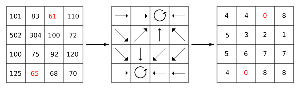
Figure 7: Flow direction algorithm

Eight neighbors algorithms are a good example of algorithm used to solve scientific problems. Indeed, it is a frequent algorithm in mathematics (finite volumes discretization), physics, image processing, geo-sciences and many other domains. However, it is not easy to make the flow direction calculation parallel with standard skeletons (map, shift etc.). Figure 8 shows the 24 skeleton calls needed. Height shift skeletons are needed to get height neighbors values, then nested calls of zipwith skeletons are needed to get the minimum value, finally map skeletons are needed to associate the minimum value to a direction.

⬇

zipwith(min,zipwith(min,zipwith(min,zipwith(min,map(f,m),

map(f,shift<1,1>(shift_id,m))),zipwith(min,

map(f,shift<1,0>(shift_id,m)),map(f,shift<1,-1>(shift_id,m)))),

zipwith(min,zipwith(min,map(f,shift<0,-1>(shift_id,m)),

map(f,shift<-1,-1>(shift_id,m))),zipwith(min,

map(f,shift<-1,0>(shift_id,m)),map(f,shift<-1,1>(shift_id,m))))),

map(f,shift<0,1>(shift_id,m)));

Figure 8: 24 nested calls needed for the flow direction calculation with standard skeletons

Then, this type of skeleton libraries have few problems :

• The difficulty of getting a parallel code is moved to the difficulty of functional programming with skeletons.

• The code is difficult to write and even more difficult to read.

• Performance damages occur because of all the skeleton calls and because of the duplication of matrices with the shift skeleton.

5.3 SkelGIS

SkelGIS is a new kind of algorithmic skeleton library. The objective is to propose a hierarchical skeleton library for very large matrices and to give access to parallelism through sequential adapted interfaces in order to keep a sequential programming style. SkelGIS gets out of the functional paradigms in order to stick to the programming habits of non-specialists. It relies on two concepts and a distributed data structure.

5.3.1 Concepts

The first concept of SkelGIS is to propose basic skeletons where the user function has a direct access to a matrix. The user has to define functions of type $f:M\longmapsto M$ ($M$ is a SkelGIS matrix).

This is a major difference with the classical skeletons (as map) where the user functions defines what to do on a single matrix element (functions of type $f:E\longmapsto E$ where $E$ is the type of elements of a matrix $m$). The user describes, in the sequential function, what to do on the matrix. As a result, the expressiveness of SkelGIS is very good and no communication skeletons are needed. SkelGIS offers a way to stay close to a sequential programming style. Another consequence of the expressiveness of basic skeletons is that a single call of skeleton at a time is needed, and performances of SkelGIS are better than existing skeletons. For example, the figure 9 gives the performances of the flow direction calculation, above-cited, with SkelGIS and SkeTo.

Size	SkeTo	SkelGIS
$339\times 225$	30ms	21ms
$14786\times 10086$	101s	31s

Figure 9: Comparison between SkeTo library and SkelGIS, on flow direction calculation

The second concept of SkelGIS is to propose a hierarchy of skeletons (Figure 10) where every higher abstraction level skeleton uses basic skeletons.

As a result, SkelGIS skeletons inherit optimizations and hardware support of basic skeletons. New optimizations or new hardware support only has to be added in basic skeletons to be available in the whole library. This hierarchy also provide a clear abstraction choice for the user. Ensuring the scalability and durability of a library is an important feature to make it live and used. Skeleton libraries are based on parallel libraries depending on hardware, and hardware can completely change quite quickly. Existing libraries propose a set of skeletons that are independent from each others. As a result, taking into account a new hardware (or a new parallel library) requires to re-implement all the skeletons of the library.

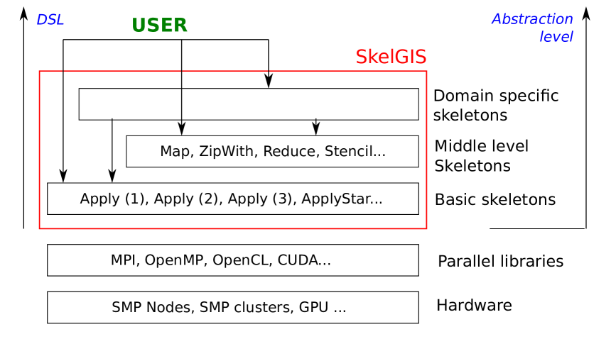
Figure 10: Hierarchy of SkelGIS

5.3.2 Distributed data structure

As every skeleton library, SkelGIS skeletons are applied to a distributed data structure. The current version of SkelGIS only proposes a distributed two-dimensional matrix to apply skeletons on. This distributed matrix named DMatrix is the basis of every parallel calculation made by SkelGIS. The constructor of the DMatrix is responsible for dividing the initial matrix in blocks and distributing the load of each block from the disk on different processors.

This DMatrix is used by skeletons to apply the user functions in parallel on the whole matrix. As the user can manipulate distributed matrices without being aware of the parallel technical details, some basic tools have been developed to manipulate them. Then, manipulation of the DMatrix looks like data structure of the Standard Template Library (STL in C++) manipulation. The three main tools to manipulate a DMatrix are:

• A set of iterators to navigate in the distributed matrix.

• A set of neighborhood functions to get the neighbors of the current element.

• Get/Set to get a value of the distributed matrix or to write a value in the distributed matrix.

The user uses the DMatrix as if it was a common sequential matrix of the STL, and the skeletons are in charge of hiding block division and communication aspects. Figures 11 and 12 represent the user code needed to get the parallel version of the flow direction calculation above-cited. The main function is in charge of the initialization of the library SkelGIS, the construction of matrices and the call of skeletons. Then, user functions have to be programmed, in a sequential programming style, using the DMatrix tools.

⬇

#include “skelgis.h”

int main(int argc, char** argv)

{

//initialization of the library

INITSKELGIS;

//creation of matrix m

DMatrix<float> * m = new DMatrix<float>(file,1);

//call of the skeleton apply with the function

// ”directions” on the matrix m

DMatrix<int> * m2 = apply<float,int>(directions,m);

//end of the library use

ENDSKELGIS;

}

Figure 11: Main function of the user program

⬇

//begin declaration of the function directions

BEGINApply(directions, input, float, output, int)

{

//initilization of iterators on input

//and output matrices

DMatrix<float>::iterator it = input->begin();

DMatrix<int>::iterator itOut = output->begin();

DMatrix<float>::iterator itEnd = input->end();

//8 neighbors table

DMatrix<float>::neighbors nghb;

//for each element of the matrix

for(; it <= itEnd; ++it , ++itOut)

{

int index=0;

//get the current value of the iterator

float min = input->getValue(it);

//get the 8 neighbor values

input->get8Neighbors(it,nghb);

//get the minimum

for(int i=0;i<8;i++){

if(nghb[i]>0 && nghb[i]<min) {

index=i+1;

min=nghb[i];}

}

//set the minimum direction in the output matrix

output->setValue(index, itOut);

}

}

//end declaration of the function

END(directions);

Figure 12: User function given to the skeleton

Behind SkelGIS, the exact same work as in MPI is done, but automatically. Actually, the library proceeds to a domain decomposition of a structured matrix and manages MPI exchanges of ghost cells at the border of the domain decomposition. Then SkelGIS proposes an easy way to code structured approaches of simulations. Of course, the structured approach is limited regarding the complexity of some simulations, but SkelGIS is under development and will propose in the future unstructured distributed data structures and also graph and tree distributed data structures. This way, SkelGIS will be able to manage different types of simulations.

6 Parallelization of FullSWOF_2D

6.1 MPI

In this section, we will explain the domain decomposition method which we have used to parallelize FullSWOF_2D (for more details see [72]). This method has been applied by using the library of functions MPI (Message Passing Interface). This method has been chosen in order to be the least intrusive as possible in the FullSWOF structure to ease future development. In fact, the domain decomposition method consists in splitting the data into many independent domains. On each domain, the code is executed by one anonymous process and when it is necessary the process communicates via calls to MPI communication primitives. MPI is a standardized and portable message-passing system used to compute on both shared memory and distributed memory machines. The parallelism with MPI decomposes into four main steps:

1. decomposition of the domain,

2. knowing his four neighbors,

3. exchanging the points on the interfaces

4. and calculating the scheme on each process.

From these four steps, we have parallelized FullSWOF_2D.

At the beginning of the run, we create a group of $n$ processes. Each process is assigned a rank between $0$ and $n-1$. For us, this linear ranking of processes is not appropriate, because the structure of the computational domain is in two dimensions with communications into the two directions. So, the processes are arranged in the 2D Cartesian topology thanks to MPI topology mechanism.

MPI creates a relationship between ranks and Cartesian coordinates and we used these information to know the neighbors of each nodes in order to communicate the values of the interfaces. After this step, the domain can be represented by a graph where the nodes stand for the processes and the edges connect process that communicate with each other. So, we can compute the number of points for each node in $x$ and $y$ and to initialize the local variables.

After the initialization, we exchange the value of the interfaces to compute the value of the variables at the next step of the time. Indeed, when we compute the value of the variables according to the order of the scheme. At order one, we add a line and column of the cells that receive the value necessary to the computation of the scheme and if we are at order two, we add two lines and two columns.

Concerning the communication between the nodes, MPI provides message-passing between any pair of processes. So, having exchanged the values at the interfaces, we compute the next step of the time by applying the algorithm of sequential FullSWOF.

6.2 SkelGIS

Using SkelGIS to parallelize the shallow water equations is very different from a standard parallelization. No parallel knowledge (domain decomposition, communications etc) and no parallel code (MPI use) are needed at all to get a parallel version of the simulation. However, the simulation has to be thought with skeleton use.

Algorithm 1 represents the pseudo code of the shallow water equations simulation and, in red is added the interventions needed to use SkelGIS with this algorithm. First, the initialization of matrices has to be made with the DMatrix object, then each algorithm step has to be executed through a skeleton call (applyList skeleton). Finally, the sequential code has to be a little modified because accesses to matrices elements have to be done through DMatrix iterators and accessors.

Initialization of variables with DMatrix

for $t\leftarrow 0$ to $N$ do

       for $i\leftarrow 0$ to $2$ do

             applyList : Boundary Conditions

             applyList : Second order reconstruction

             applyList : Hydrostatic reconstruction

             applyList : Numerical flux computation

             applyList : Scheme computation

             applyList : Frictions

       end for

      applyList : Order 2 along $t$ - Method of Heun

end for

Algorithm 1 Shallow water equations algorithm with additional calls in red for SkelGIS

In addition to the fact that no parallelization knowledge is needed using SkelGIS, the non-computing scientist is fully independent in parallel developments. The parallel application getting from the use of SkelGIS is organized and easily upgradeable. Furthermore, an OpenMP version and the use of SSE instructions (Streaming SIMD extensions) optimizations are under development in SkelGIS. As a result with no efforts the code of shallow water equations will work with OpenMP for shared memory systems as with Intel additional processor instructions.

6.3 Results

In this part are presented some comparison results between the MPI implementation and the SkelGIS implementation of the shallow water equations. These benchmarks were made on a 5120x5120 domain with 5000 iterations and 20.000 iterations. Figures 13 and 14 represent the base two logarithm of the execution times. Then, it represents the inverse of the speedup and the ideal execution time is drawn in blue.

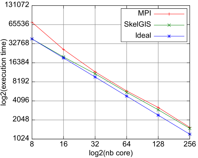
Figure 13: Comparison between MPI, SkelGIS and Ideal versions of shallow water equations for 5000 time iterations : Log 2 of execution times

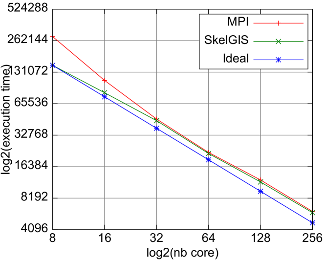
Figure 14: Comparison between MPI, SkelGIS and Ideal versions of shallow water equations for 20000 time iterations : Log 2 of execution times

Both implementations have very good results and are closed to the ideal execution time. We can notice, however, that SkelGIS results are linear while the MPI version starts with a bigger execution time with 8 processors. From 32 to 256 processors the MPI implementation meets SkelGIS execution times.

Conclusions

As a conclusion, both implementations are efficient, but parallelization concepts of these two implementations are very different. The Skeletton strategy requires a more important work to rewrite the code, using SKELGIS library but it provides a final code with a greater expressivity and the parallelization technics are hidden within the library. On the contrary, the MPI version involves less changes in the software, but it requires to deal with the parallelization concept. Therefore, our first conclusion is that the performances of the two approaches are very close. For an existing code, depending on the skills of the developers, each strategy can be preferred. If the choice is done at the very beginning of the project, skeletons offers a more expressive code and does not require to know about parallelization. Both FullSWOF_2D and SKELGIS are still under development, interested readers might contact us for further informations.

References

- [1] R. Moussa and C. Bocquillon, “Approximation zones of the Saint-Venant equations for flood routing with overbank flow,” Hydrology and Earth System Sciences, vol. 4, no. 2, pp. 251–261, 2000.
- [2] P. Novak, V. Guinot, A. Jeffrey, and D. E. Reeve, Hydraulic modelling – an Introduction. Spoon Press, 2010.
- [3] W. Zhang and T. W. Cundy, “Modeling of two-dimensional overland flow,” Water Resources Research, vol. 25, no. 9, pp. 2019–2035, Sep. 1989.
- [4] M. Esteves, X. Faucher, S. Galle, and M. Vauclin, “Overland flow and infiltration modelling for small plots during unsteady rain : numerical results versus observed values,” Journal of Hydrology, vol. 228, pp. 265–282, 2000.
- [5] R. F. Fiedler and J. A. Ramirez, “A numerical method for simulating discontinuous shallow flow over an infiltrating surface,” International Journal for Numerical Methods in Fluids, vol. 32, pp. 219–240, 2000.
- [6] A. J.-C. de Saint Venant, “Théorie du mouvement non-permanent des eaux, avec application aux crues des rivières et à l’introduction des marées dans leur lit,” Comptes Rendus de l’Académie des Sciences, vol. 73, pp. 147–154, 1871.
- [7] J. M. Greenberg and A.-Y. LeRoux, “A well-balanced scheme for the numerical processing of source terms in hyperbolic equation,” SIAM Journal on Numerical Analysis, vol. 33, pp. 1–16, 1996.
- [8] M. Rousseau, O. Cerdan, O. Delestre, F. Dupros, F. James, and S. Cordier, “Overland flow modelling with shallow water equation using well balanced numerical scheme: Adding efficiency or just more complexity ?” submitted. [Online]. Available: http://hal.archives-ouvertes.fr/hal-00664535
- [9] J. A. Cunge and M. Wegner, “Intégration numérique des équations d’écoulement de barré de Saint-Venant par un schéma implicite de différences finies,” La Houille Blanche, no. 1, pp. 33–39, 1964. [Online]. Available: http://dx.doi.org/10.1051/lhb/1964002
- [10] J. A. Cunge, F. M. Holly Jr., and A. Verwey, Practical Aspects of Computational River Hydraulics, reprint Iowa University Press, Ed. Pitman Publisher, 1980.
- [11] O. Delestre, “Simulation du ruissellement d’eau de pluie sur des surfaces agricoles/ rain water overland flow on agricultural fields simulation,” Ph.D. dissertation, Université d’Orléans (in French), available from TEL: tel.archives-ouvertes.fr/INSMI/tel-00531377/fr, Jul. 2010.
- [12] W. H. Green and G. A. Ampt, “Studies on soil physics,” The Journal of Agricultural Science, vol. 4, pp. 1–24, 1911.
- [13] O. Delestre, C. Lucas, P.-A. Ksinant, F. Darboux, C. Laguerre, T.-N.-T. Vo, F. James, and S. Cordier, “SWASHES: a compilation of shallow water analytic solutions for hydraulic and environmental studies,” International Journal for Numerical Methods in Fluids, vol. 72, no. 3, pp. 269–300, 2013. [Online]. Available: http://dx.doi.org/10.1002/fld.3741
- [14] O. Delestre, S. Cordier, F. Darboux, M. Du, F. James, C. Laguerre, C. Lucas, and O. Planchon, “FullSWOF: A software for overland flow simulation,” in SIMHYDRO 2012 – New Frontiers of Simulation, ser. Springer Hydrogeology, P. Gourbesville, J. Cunge, and G. Caignaert, Eds. Advances in Hydroinformatics, 2014, p. 450.
- [15] L. Tatard, O. Planchon, J. Wainwright, G. Nord, D. Favis-Mortlock, N. Silvera, O. Ribolzi, M. Esteves, and C.-H. Huang, “Measurement and modelling of high-resolution flow-velocity data under simulated rainfall on a low-slope sandy soil,” Journal of Hydrology, vol. 348, no. 1-2, pp. 1–12, jan 2008.
- [16] N. Goutal and F. Maurel, “A finite volume solver for 1D shallow-water equations applied to an actual river,” International Journal for Numerical Methods in Fluids, vol. 38, pp. 1–19, 2002.
- [17] J. Burguete and P. Garcìa-Navarro, “Implicit schemes with large time step for non-linear equations : application to river flow hydraulics,” International Journal for Numerical Methods in Fluids, vol. 46, pp. 607–636, 2004.
- [18] V. Caleffi, A. Valiani, and A. Zanni, “Finite volume method for simulating extreme flood events in natural channels,” Journal of Hydraulic Research, vol. 41, no. 2, pp. 167–177, 2003.
- [19] O. Delestre, S. Cordier, F. James, and F. Darboux, “Simulation of rain-water overland-flow,” in Proceedings of the 12th International Conference on Hyperbolic Problems, University of Maryland, College Park (USA), 2008, E. Tadmor, J.-G. Liu and A. Tzavaras Eds., Proceedings of Symposia in Applied Mathematics 67, Amer. Math. Soc., 537–546, 2009.
- [20] F. Alcrudo and E. Gil, “The Malpasset dam break case study,” in the CADAM Workshop, Zaragoza, Nov. 1999, pp. 95–109.
- [21] A. Valiani, V. Caleffi, and A. Zanni, “Case study : Malpasset dam-break simulation using a two-dimensional finite volume methods,” Journal of Hydraulic Engineering, vol. 128, no. 5, pp. 460–472, May 2002.
- [22] A. G. L. Borthwick, S. Cruz León, and J. Józsa, “The shallow flow equations solved on adaptative quadtree grids,” International Journal for Numerical Methods in Fluids, vol. 37, pp. 691–719, 2001.
- [23] F. Marche, “Theoretical and numerical study of shallow water models. applications to nearshore hydrodynamics,” Ph.D. dissertation, Laboratoire de mathématiques appliquées – université de Bordeaux 1, Dec. 2005.
- [24] D. L. George, “Finite volume methods and adaptive refinement for tsunami propagation and inundation,” Ph.D. dissertation, University of Washington, 2006.
- [25] D.-H. Kim, Y.-S. Cho, and Y.-K. Yi, “Propagation and run-up of nearshore tsunamis with HLLC approximate Riemann solver,” Ocean Engineering, vol. 34, no. 8-9, pp. 1164–1173, 2007. [Online]. Available: http://www.sciencedirect.com/science/article/B6V4F-4M6SGFH-1/2/161a433e%70388fb34b99c58495ea599f
- [26] S. Popinet, “Quadtree-adaptative tsunami modelling,” Ocean Dynamics, pp. 1–25, May 2011.
- [27] M.-H. Le, “Modélisation multi échelle et simulation numérique de l’érosion des sols de la parcelle au bassin versant,” Ph.D. dissertation, Université d’Orléans, Nov. 2012.
- [28] L. A. Richards, “Capillary conduction of liquids through porous mediums,” Physics, vol. 1, pp. 318–333, Nov. 1931.
- [29] V. T. Chow, Open-Channel Hydraulics, N. York, Ed. McGraw-Hill, 1959.
- [30] M.-O. Bristeau and B. Coussin, “Boundary conditions for the shallow water equations solved by kinetic schemes,” INRIA, Tech. Rep. 4282, Oct. 2001.
- [31] M.J. Castro, A. Pardo and C. Parès, “Well-balanced numerical schemes based on a generalized hydrostatic reconstruction technique,” Mathematical Models and Methods in Applied Sciences, vol. 17, no. 12, pp. 2065–2113, 2007.
- [32] A. Bermúdez and M. E. Vázquez, “Upwind methods for hyperbolic conservation laws with source terms,” Computers & Fluids, vol. 23, no. 8, pp. 1049–1071, 1994. [Online]. Available: http://www.sciencedirect.com/science/article/B6V26-47YMXJT-16/2/4485b4a%db616198b768daff172258660
- [33] A. Bermúdez, A. Dervieux, J.-A. Desideri, and M. E. Vázquez, “Upwind schemes for the two-dimensional shallow water equations with variable depth using unstructured meshes,” Computer Methods in Applied Mechanics and Engineering, vol. 155, no. 1-2, pp. 49–72, 1998. [Online]. Available: http://www.sciencedirect.com/science/article/B6V29-3WN739F-4/2/3120ee07%ea5c43b3318fbfb6c05d2dde
- [34] R. J. LeVeque, “Balancing source terms and flux gradients in high-resolution Godunov methods: The quasi-steady wave-propagation algorithm,” Journal of Computational Physics, vol. 146, no. 1, pp. 346–365, 1998. [Online]. Available: http://www.sciencedirect.com/science/article/B6WHY-45J58TW-22/2/72a8af8%c9e23f63b0df9484475f7e2df
- [35] S. Jin, “A steady-state capturing method for hyperbolic systems with geometrical source terms,” M2AN, vol. 35, no. 4, pp. 631–645, Jul. 2001. [Online]. Available: http://dx.doi.org/10.1051/m2an:2001130
- [36] A. Kurganov and D. Levy, “Central-upwind schemes for the Saint-Venant system,” Mathematical Modelling and Numerical Analysis, vol. 36, pp. 397–425, 2002.
- [37] T. Gallouët, J.-M. Hérard, and N. Seguin, “Some approximate Godunov schemes to compute shallow-water equations with topography,” Computers & Fluids, vol. 32, pp. 479–513, 2003.
- [38] E. Audusse, F. Bouchut, M.-O. Bristeau, R. Klein, and B. Perthame, “A fast and stable well-balanced scheme with hydrostatic reconstruction for shallow water flows,” SIAM J. Sci. Comput., vol. 25, no. 6, pp. 2050–2065, 2004.
- [39] E. Audusse and M.-O. Bristeau, “A well-balanced positivity preserving ”second-order” scheme for shallow water flows on unstructured meshes,” Journal of Computational Physics, vol. 206, pp. 311–333, 2005.
- [40] S. Noelle, Y. Xing, and C. W. Shu, “High-order well-balanced finite volume WENO schemes for shallow water equation with moving water,” Journal of Computational Physics, vol. 226, no. 1, pp. 29–58, 2007. [Online]. Available: http://www.sciencedirect.com/science/article/B6WHY-4NG3TH4-3/2/546ff3d2%47ae9db8ed41e3de935ee892
- [41] Q. Liang and F. Marche, “Numerical resolution of well-balanced shallow water equations with complex source terms,” Advances in Water Resources, vol. 32, no. 6, pp. 873–884, 2009. [Online]. Available: http://www.sciencedirect.com/science/article/B6VCF-4VR9FHT-3/2/5218868d%cfded7d34380666f23000855
- [42] C. Berthon and F. Foucher, “Efficient well-balanced hydrostatic upwind schemes for shallow-water equations,” Journal of Computational Physics, vol. 231, pp. 4993–5015, 2012.
- [43] F. Bouchut, Nonlinear stability of finite volume methods for hyperbolic conservation laws, and well-balanced schemes for sources, B. Basel, Ed. Birkhäuser Basel, 2004, vol. 2/2004.
- [44] B. van Leer, “Towards the ultimate conservative difference scheme. V. A second-order sequel to Godunov’s method,” Journal of Computational Physics, vol. 32, no. 1, pp. 101–136, 1979. [Online]. Available: http://www.sciencedirect.com/science/article/B6WHY-4DD1N8T-C5/2/9b051d1%cfcff715a3d0f4b7b7b0397cc
- [45] C.-W. Shu and S. Osher, “Efficient implementation of essentially non-oscillatory shock-capturing schemes,” Journal of Computational Physics, vol. 77, no. 2, pp. 439–471, 1988. [Online]. Available: http://www.sciencedirect.com/science/article/B6WHY-4DD1T6W-MM/2/bef99e4%b67bd7132c8af1984c34ce57e
- [46] A. Harten, P. D. Lax, and B. van Leer, “On upstream differencing and godunov-type schemes for hyperbolic conservation laws,” SIAM Review, vol. 25, no. 1, pp. 35–61, Jan. 1983.
- [47] P. Batten, N. Clarke, C. Lambert and D.M. Causon, “On the Choice of Wavespeeds for the HLLC Riemann Solver,” SIAM J. Sci. Comput., vol. 18, no. 6, pp. 1553–1570, 1997. [Online]. Available: http://dx.doi.org/10.1137/S1064827593260140
- [48] A. Goubet, “Risques associés aux barrages/ risks associated with storage dams,” La Houille Blanche, vol. 8, pp. 475–490, 1979.
- [49] A. Lebreton, “Les ruptures et accidents graves de barrages de 1964 à 1983/ ruptures and serious accidents on dams from 1964 to 1983,” La Houille Blanche, vol. 6-7, pp. 529–544, 1985.
- [50] G. Benoist, “Les études d’ondes de submersion des grands barrages d’EDF,” La Houille Blanche, vol. 1, pp. 43–54, 1989.
- [51] A. Gioda, C. Serrano, and A. Forenza, “Les ruptures de barrages dans le monde : un nouveau bilan de Potosi (1626, Bolivie)/ dam collapses in the world: a new estimation of the Potosi disaster (1626, Bolivia),” La Houille Blanche, vol. 4-5, pp. 165–170, 2002.
- [52] H. Chanson, “Applications of the Saint-Venant equations and method of characteristics to the dam break wave problem,” Report No. CH55/05, vol. Dept. of Civil Engineering, The University of Queensland, Brisbane, Australia, May, p. 135 pages, May 2005.
- [53] ——, “Solutions analytiques de l’onde de rupture de barrage sur plan horizontal et incliné,” La Houille Blanche, no. 3, pp. 76–86, 2006.
- [54] T. Mulder, S. Zaragosi, J.-M. Jouanneau, G. Bellaiche, S. Guérinaud, and J. Querneau, “Deposits related to the failure of the Malpasset dam in 1959 an analogue for hyperpycnal deposits from jökulhlaups,” Marine Geology, vol. 260, pp. 81–89, 2009.
- [55] J.-M. Hervouet, “TELEMAC, a hydroinformatic system/ Télémac, un système hydroinformatique,” La Houille Blanche, vol. 3-4, pp. 21–28, 1999.
- [56] ——, “A high resolution 2-d dam-break model using parallelization,” Hydrological Processes, vol. 14, pp. 2211–2230, 2000.
- [57] N. Malleron, F. Zaoui, N. Goutal, and T. Morel, “On the use of a high-performance framework for efficient model coupling in hydroinformatics,” Environmental Modelling & Software, vol. 26, pp. 1747–1758, 2011.
- [58] J. Singh, M. S. Altinakar, and Y. Ding, “Two-dimensional numerical modeling of dam-break flows over natural terrain using a central explicit scheme,” Advances in Water Resources, vol. 34, pp. 1366–1375, 2011.
- [59] A. Duran, Q. Liang, and F. Marche, “On the well-balanced numerical discretization of shallow water equations on unstructured meshes,” Journal of Computational Physics, 2012.
- [60] R. Ata, S. Pavan, S. Khelladi, and E. F. Toro, “A Weighted Average Flux (WAF) scheme for the shallow water equations with friction and real topography,” submitted.
- [61] J.-M. Hervouet, Hydrodynamics of free surface flows: Modelling with the finite element Method, J. W. . Sons, Ed., 2007.
- [62] V. Kumar, Introduction to parallel computing, 2nd ed. Boston, MA, USA: Addison-Wesley Longman Publishing Co., Inc., 2002.
- [63] M. I. Cole, “Algorithmic skeletons: a structured approach to the management of parallel computation,” Ph.D. dissertation, 1988, aAID-85022.
- [64] A. Benoit and M. Cole, “Two fundamental concepts in skeletal parallel programming,” in Proceedings of the 5th international conference on Computational Science - Volume Part II, ser. ICCS’05. Berlin, Heidelberg: Springer-Verlag, 2005, pp. 764–771.
- [65] M. Cole, “Bringing skeletons out of the closet: a pragmatic manifesto for skeletal parallel programming,” Parallel Comput., vol. 30, pp. 389–406, March 2004. [Online]. Available: http://dl.acm.org/citation.cfm?id=1007980.1007985
- [66] J. Falcou, J. Sérot, T. Chateau, and J.-T. Lapresté, “QUAFF: efficient C++ design for parallel skeletons,” Parallel Computing, vol. 32, no. 7-8, pp. 604–615, 2006.
- [67] A. Benoit, M. Cole, S. Gilmore, and J. Hillston, “Flexible skeletal programming with eskel,” in Euro-Par, 2005, pp. 761–770.
- [68] G. H. Botorog and H. Kuchen, “Efficient parallel programming with algorithmic skeletons,” in Euro-Par, Vol. I, 1996, pp. 718–731.
- [69] K. Matsuzaki, H. Iwasaki, K. Emoto, and Z. Hu, “A library of constructive skeletons for sequential style of parallel programming,” in Infoscale, 2006, p. 13.
- [70] N. Javed and F. Loulergue, “A formal programming model of Orléans skeleton library,” in PaCT, 2011, pp. 40–52.
- [71] U. Gruber and P. Bartelt, “Snow avalanche hazard modelling of large areas using shallow water numerical methods and {GIS},” Environmental Modelling & Software, vol. 22, no. 10, pp. 1472–1481, 2007. [Online]. Available: http://www.sciencedirect.com/science/article/pii/S1364815207000023
- [72] I. Brugeas. (1996, March) Utilisation de MPI en décomposition de domaine. CNRS–IDRIS. [Online]. Available: http://www.idris.fr/data/publications/mpi.ps