Linear Precoder Design for MIMO Interference Channels with Finite-Alphabet Signaling

Yongpeng Wu,  Chengshan Xiao,  Xiqi Gao, ,
John D. Matyjas, , and Zhi Ding
Manuscript received Feb. 15, 2013; revised May 26, 2013. The associate editor coordinating the review of this paper and approving it for publication was Tony Q. S. Quek.Part of the material in this paper will be presented at IEEE GLOBECOM 2013. The work of Y. Wu and X. Gao was supported in part by National Natural Science Foundation of China under Grants 60925004 and 61222102, the China High-Tech 863 Plan under Grant 2012AA01A506, and National Science and Technology Major Project of China under Grants 2011ZX03003-001 and 2011ZX03003-003-03. The work of C. Xiao was supported in part by National Science Foundation under Grants CCF-0915846 and ECCS-1231848. The work of Z. Ding was supported by NSF Grants 0917251 and 1147930. This work began while Y. Wu was a visiting Missouri University of Science and Technology and was completed while C. Xiao was a summer faculty fellow at the Air Force Research Laboratory in Rome, NY. Approved for Public Release; Distribution Unlimited: 88ABW-2013-1062. ACKNOWLEDGMENT OF SUPPORT AND DISCLAIMER: (a) Contractor acknowledges Government’s support in the publication of this paper. This material is based upon work funded by the AF Summer Faculty Fellow Program, under AFRL Contract No. FA8750-11-2-0218. (b) Any opinions, findings and conclusions or recommendations expressed in this material are those of the author(s) and do not necessarily reflect the views of AFRL.Y. Wu and X. Gao are with the National Mobile Communications Research Laboratory, Southeast University, Nanjing, 210096, P. R. China (Email: ypwu@seu.edu.cn; xqgao@seu.edu.cn). C. Xiao is with the Department of Electrical and Computer Engineering, Missouri University of Science and Technology, Rolla, MO 65409, USA (Email: xiaoc@mst.edu). J. D. Matyjas is with the Air Force Research Laboratory/RIT, Rome, NY 13441, USA (E-mail: John.Matyjas@rl.af.mil).Z. Ding is with the Department of Electrical and Computer Engineering, University of California, Davis, CA 95616, USA (Email: zding@ucdavis.ca).
Abstract

This paper investigates the linear precoder design for K𝐾K-user interference channels of multiple-input multiple-output (MIMO) transceivers under finite alphabet inputs. We first obtain general explicit expressions of the achievable rate for users in the MIMO interference channel systems. We study optimal transmission strategies in both low and high signal-to-noise ratio (SNR) regions. Given finite alphabet inputs, we show that a simple power allocation design achieves optimal performance at high SNR whereas the well-known interference alignment technique for Gaussian inputs only utilizes a partial interference-free signal space for transmission and leads to a constant rate loss when applied naively to finite-alphabet inputs. Moreover, we establish necessary conditions for the linear precoder design to achieve weighted sum-rate maximization. We also present an efficient iterative algorithm for determining precoding matrices of all the users. Our numerical results demonstrate that the proposed iterative algorithm achieves considerably higher sum-rate under practical QAM inputs than other known methods.

Index Terms:
Finite alphabet, interference channel, linear precoding, MIMO

I Introduction

The recent decade has witnessed the widespread application of multiple-input multiple-output (MIMO) wireless communication systems because of their superb spectral efficiency and link reliability [1, 2, 3]. However, potential benefits of MIMO systems are often hampered by the omni-present interference in typical scenarios of wireless networks [4, 7, 5, 6]. For this reason, considerable research interests have focused on MIMO interference channels recently. Unlike the general tendency to assume Gaussian signal inputs in such works, our paper here investigates linear precoding of K𝐾K-user MIMO interference channel systems for finite alphabet input signals.

Although there have been substantial progresses in information-theoretical analysis of Gaussian interference channels in some special cases [8, 9, 10], the fundamental limits of the interference channels still remain unresolved in general [11]. A more recent signal multiplexing approach, called interference alignment (IA), has shown that the degrees of freedom (DOF) of the interference channels may be achieved in high signal-to-noise ratio (SNR) region [12]. The IA concept has been extended to MIMO interference channel systems [13, 14]. Furthermore, linear precoding designs maximizing the weighted sum-rate (WSR) performance of the MIMO interference channel systems in moderate SNR region can be found in [15].

Nevertheless, the aforementioned information-theoretic works attempt to optimize the performance of interference channel systems by relying on the convenience of Gaussian input assumption. Despite the information-theoretic optimality of Gaussian inputs, practical communication systems rarely transmit Gaussian signals. It is well known that practical signals usually are generated from finite discrete constellation sets such as phase-shift keying (PSK), pulse-amplitude modulation (PAM), or quadrature amplitude modulation (QAM). MIMO precoders designed for Gaussian input assumption may often lead to a considerable performance loss when applied haphazardly to practical systems with finite alphabet signaling. We take point-to-point case as an example. For QPSK modulation, as illustrated in Figure 2 and Figure 4 in [16], the performance gaps between the finite alphabet input design and the Gaussian input design are more than 151515 dB at 0.750.750.75 coding rate.

Thus, transmitter designs for optimizing the constellation-constrained mutual information appear more plausible in practice. Such problems in the context of point-to-point communication scenarios [17, 18, 16, 19] have been recently studied. Precoding designs in multiple access channels, broadcast channels, relay channels, and wiretap channels have also appeared [20, 21, 22, 23, 24, 25]. In [26], a transmit precoding design for two user single-input single-output (SISO) strong interference channels with finite alphabet inputs was proposed. It was suggested in [26] to design the precoders by an exhaust search for the optimal rotation of the signal constellation at the second user side.

To the best of our knowledge, not much has been published on the MIMO interference channel systems under finite alphabet constraints. This paper considers the linear precoder designs to maximize the WSR of the MIMO interference channel systems under finite alphabet constraints of channel inputs. Our results differ significantly from previous finite alphabet research work since the existing results on the MIMO multiuser systems with finite alphabet inputs [21, 23] cannot be directly applied to the MIMO interference channel systems. Besides, new insights of the precoding designs over MIMO interference channels in asymptotic SNR regions are revealed. Moreover, a novel receiver structure exploiting the finite discrete constellation set is provided. The specific contributions of this paper can be summarized as follows. Based on the mutual information between the channel input and output, we first derive an exact expressions of the achievable rate of each user in the MIMO interference channel systems with finite alphabet inputs. The characterization is applicable to Klimit-from𝐾K-users with generic antenna configurations. We then find a near-optimal transmission strategy in low SNR region, where each user performs beamforming in the strongest eigenmode of its channel matrix. This transmission design coincides with the low-SNR optimal precoding policy in the point-to-point MIMO scenarios and also for Gaussian inputs. At high SNR, however, the precoding design with finite alphabet inputs is significantly different from that with Gaussian inputs. For Gaussian input, the optimal IA technique [13, 15] constructs the precoder of each transmitter by properly aligning interference of each receiver to a partial signal space. The remaining interference-free space is utilized for signal transmissions. However, when replaced with finite alphabet inputs, the IA technique may lead to a serious performance loss111For Gaussian input case, it is well known that the IA technique achieves the optimal DOF in high SNR region. The high SNR analysis in our paper reveals that this conclusion fails to hold for finite alphabet inputs theoretically. We admit that even for Gaussian input, the IA technique may still result in gaps from the actual rates at finite SNR levels. Therefore, the linear precoding design over interference channels with Gaussian input for arbitrary SNR values [15] will also be simulated and compared in order to report actual performance gaps at finite SNR levels.. This is because finite alphabet inputs lead to saturated mutual information. Thus, allocating more power to signals of high SNR beyond saturation does not further increase mutual information. This means that using only a partial signal space for transmitting signals will result in a constant sum-rate loss in finite alphabet input scenarios. For example, if each transmitter has NTsubscript𝑁𝑇N_{T} antenna and each receiver has NRsubscript𝑁𝑅N_{R} antenna, we prove that the IA technique will result in (η+1)1j=1Klog2Mjsuperscript𝜂11superscriptsubscript𝑗1𝐾subscript2subscript𝑀𝑗(\eta+1)^{-1}\sum\nolimits_{j=1}^{K}{\log_{2}M_{j}} b/s/Hz sum-rate loss at high SNR, where Mjsubscript𝑀𝑗M_{j} denotes the size of the modulation set and η𝜂\eta depends on the ratio of NRsubscript𝑁𝑅N_{R} and NTsubscript𝑁𝑇N_{T}.

As a consequence, instead of the IA, we propose a novel and concise power allocation scheme exploiting the full signal space for signal transmission at high SNR. Our scheme applies to arbitrary number of users and arbitrary antenna configurations. We prove that the proposed scheme can effectively combat interference and achieve the saturated sum-rate j=1Klog2Mjsuperscriptsubscript𝑗1𝐾subscript2subscript𝑀𝑗\sum\nolimits_{j=1}^{K}{\log_{2}M_{j}} b/s/Hz at high SNR. More generally, due to the non-convexity of the WSR with respect to the precoding matrices, we derive a set of necessary conditions for the optimal precoding matrices through Karush-Kuhn-Tucker (KKT) analysis and further propose an iterative algorithm using gradient descent and backtracking line search for finding the optimal precoders. Numerical results show that the proposed algorithm converges within several steps and achieves significant WSR gains over the conventional iterative designs. In addition to WSR, the coded bit error rate (BER) of the MIMO interference channel systems is another important performance evaluation criterion in practice. To further examine the robust performance of the proposed design, we present iterative transceiver systems for the MIMO interference channels by deploying low-density parity-check (LDPC) encoders and the proposed precoders at the transmitters, and the soft maximum a posteriori (MAP) multiuser detectors and LDPC decoders at the receivers. Simulations show that the proposed precoding design achieves substantial coded BER improvement through the iterative decoding and detection operations. Furthermore, recognizing interference signals as finite alphabet inputs rather than colored Gaussian noise, we designed a novel detector structure that provides additional coded BER gains.

The following notations are adopted throughout the paper: Column vectors are represented by lower-case bold-face letters, and matrices are represented using upper-case bold-face letters. Superscripts ()Tsuperscript𝑇(\cdot)^{T}, ()superscript(\cdot)^{*}, and ()Hsuperscript𝐻(\cdot)^{H} represent the matrix/vector transpose, conjugate, and conjugate-transpose operations, respectively. We let 𝐱norm𝐱\left\|{\mathbf{x}}\right\| and 𝐗Fsubscriptnorm𝐗𝐹\left\|{\mathbf{X}}\right\|_{F} denote the Euclidean norm of vector 𝐱𝐱{\mathbf{x}} and the Frobenius norm of matrix 𝐗𝐗\mathbf{X}, respectively. \mathbb{C} denotes the complex field. 𝐈Msubscript𝐈𝑀{\mathbf{I}}_{M} denotes an M×M𝑀𝑀M\times M identity matrix (sometimes without using subscript M𝑀M) and EVsubscript𝐸𝑉E_{V} represents the expectation of random variable (scalar, vector, or matrix) V𝑉V.

II System Model and Existing Results of MIMO Interference Channel With Gaussian Inputs

We consider a K𝐾K-user interference channel system in which each transmitter has dedicated information for its intended receiver and generates co-channel interference to other receivers as illustrated in Figure 1. Suppose the i𝑖i-th transmitter has Ntisubscript𝑁subscript𝑡𝑖N_{t_{i}} antennas and the j𝑗j-th receiver has Nrjsubscript𝑁subscript𝑟𝑗N_{r_{j}} antennas for every i,j=1,2,,Kformulae-sequence𝑖𝑗12𝐾i,j=1,2,\cdots,K. In addition, we assume no collaboration among transmitters or receivers. Then, the received signal 𝐲jNrj×1subscript𝐲𝑗superscriptsubscript𝑁subscript𝑟𝑗1{\bf{y}}_{j}\in\mathbb{C}^{N_{r_{j}}\times 1} observed at the j𝑗j-th receiver can be described as

𝐲j=𝐇jj𝐆j𝐱j+i=1,ijK𝐇ji𝐆i𝐱i+𝐧j,j=1,2,,Kformulae-sequencesubscript𝐲𝑗subscript𝐇𝑗𝑗subscript𝐆𝑗subscript𝐱𝑗superscriptsubscriptformulae-sequence𝑖1𝑖𝑗𝐾subscript𝐇𝑗𝑖subscript𝐆𝑖subscript𝐱𝑖subscript𝐧𝑗𝑗12𝐾{\bf{y}}_{j}={\bf{H}}_{jj}{\bf{G}}_{j}{\mathbf{x}}_{j}+\sum\limits_{i=1,i\neq j}^{K}{{\bf{H}}_{ji}{\bf{G}}_{i}{\bf{x}}_{i}}+{\bf{n}}_{j},\ j=1,2,\cdots,K (1)

where 𝐱jNtj×1subscript𝐱𝑗superscriptsubscript𝑁subscript𝑡𝑗1{\mathbf{x}}_{j}\in\mathbb{C}^{N_{t_{j}}\times 1} and 𝐧jNrj×1subscript𝐧𝑗superscriptsubscript𝑁subscript𝑟𝑗1{\mathbf{n}}_{j}\in\mathbb{C}^{N_{r_{j}}\times 1} denote the zero-mean transmitted information vector and noise vector for the j𝑗j-th user with covariance matrices 𝐈𝐈\mathbf{I} and σ2𝐈superscript𝜎2𝐈\sigma^{2}\mathbf{I}, respectively. Also, 𝐆jsubscript𝐆𝑗{\mathbf{G}}_{j} represents the linear precoding matrix for the j𝑗j-th user, and 𝐇jiNrj×Ntisubscript𝐇𝑗𝑖superscriptsubscript𝑁subscript𝑟𝑗subscript𝑁subscript𝑡𝑖{\mathbf{H}}_{ji}\in\mathbb{C}^{N_{r_{j}}\times N_{t_{i}}} stands for the channel response matrix between the i𝑖i-th transmitter and the j𝑗j-th receiver, which is normalized as tr(𝐇ji𝐇jiH)=Nrjtrsubscript𝐇𝑗𝑖superscriptsubscript𝐇𝑗𝑖𝐻subscript𝑁subscript𝑟𝑗\text{tr}\left({{\mathbf{H}}_{ji}{\mathbf{H}}_{ji}^{H}}\right)=N_{r_{j}}. Here we make the common assumption (e.g., as in [12, 15], among others) that the channel state information is globally available, i.e., each transmitter has access to perfect channel knowledge of all users. Moreover, we assume the precoding matrix does not increase the transmission power. Henceforth, we have the power constraint

tr(E[𝐆j𝐱j𝐱jH𝐆jH])=tr(𝐆j𝐆jH)Pj,j=1,2,,Kformulae-sequencetr𝐸delimited-[]subscript𝐆𝑗subscript𝐱𝑗superscriptsubscript𝐱𝑗𝐻superscriptsubscript𝐆𝑗𝐻trsubscript𝐆𝑗superscriptsubscript𝐆𝑗𝐻subscript𝑃𝑗𝑗12𝐾\text{tr}\left({E\left[{{\bf{G}}_{j}{\bf{x}}_{j}{\bf{x}}_{j}^{H}{\bf{G}}_{j}^{H}}\right]}\right)=\text{tr}\left({{\bf{G}}_{j}{\bf{G}}_{j}^{H}}\right)\leq P_{j},\ j=1,2,\cdots,K (2)

where Pjsubscript𝑃𝑗P_{j} denotes the maximum average transmitted power at the j𝑗j-th transmitter.

\psfrag{1}{\tiny$1$}\psfrag{2}{\tiny$2$}\psfrag{K}{\tiny$K$}\psfrag{x_1}{\scriptsize$\mathbf{x}_{1}$}\psfrag{x_2}{\scriptsize$\mathbf{x}_{2}$}\psfrag{x_K}{\scriptsize$\mathbf{x}_{\tiny{K}}$}\psfrag{G_1}{\scriptsize$\mathbf{G}_{1}$}\psfrag{G_2}{\scriptsize$\mathbf{G}_{2}$}\psfrag{G_K}{\scriptsize$\mathbf{G}_{K}$}\psfrag{{H_ij}}{\scriptsize$\mathbf{H}_{ij}$}\psfrag{x_1_out}{\scriptsize$\mathbf{x}_{1,\rm{out}}$}\psfrag{x_2_out}{\scriptsize$\mathbf{x}_{2,\rm{out}}$}\psfrag{x_K_out}{\scriptsize$\mathbf{x}_{K,\rm{out}}$}\includegraphics[width=195.12767pt]{Fig1}
Figure 1: K𝐾K-user interference channels with multiple antennas.

We now briefly review the existing linear precoding design in the MIMO interference channel systems based on Gaussian input assumption. When 𝐱j𝒞𝒩(0,𝐈Ntj),j=1,2,,Kformulae-sequencesimilar-tosubscript𝐱𝑗𝒞𝒩0subscript𝐈subscript𝑁subscript𝑡𝑗𝑗12𝐾{\mathbf{x}}_{j}\sim{\cal CN}(0,\;{\bf{I}}_{N_{t_{j}}}),j=1,2,\cdots,K, the achievable rate for the j𝑗j-th user is given by [15]

Rj=log2det(σ2𝐈+i=1K𝐇ji𝐆i𝐆iH𝐇jiH)log2det(σ2𝐈+i=1,ijK𝐇ji𝐆i𝐆iH𝐇jiH).subscript𝑅𝑗subscript2superscript𝜎2𝐈superscriptsubscript𝑖1𝐾subscript𝐇𝑗𝑖subscript𝐆𝑖superscriptsubscript𝐆𝑖𝐻superscriptsubscript𝐇𝑗𝑖𝐻subscript2superscript𝜎2𝐈superscriptsubscriptformulae-sequence𝑖1𝑖𝑗𝐾subscript𝐇𝑗𝑖subscript𝐆𝑖superscriptsubscript𝐆𝑖𝐻superscriptsubscript𝐇𝑗𝑖𝐻\begin{array}[]{l}R_{j}=\log_{2}\det\left(\sigma^{2}{{\bf{I}}+\sum\limits_{i=1}^{K}{{\bf{H}}_{ji}{\bf{G}}_{i}{\bf{G}}_{i}^{H}{\bf{H}}_{ji}^{H}}}\right)\\ \qquad\qquad-\log_{2}\det\left({\sigma^{2}{\bf{I}}+\sum\limits_{i=1,i\neq j}^{K}{{\bf{H}}_{ji}{\bf{G}}_{i}{\bf{G}}_{i}^{H}{\bf{H}}_{ji}^{H}}}\right).\end{array} (3)

Therefore, the optimum precoding matrices for maximizing the WSR can be expressed as

{𝐆1,𝐆2,,𝐆K}=argmax𝐆1,𝐆2,,𝐆KRwsumsuperscriptsubscript𝐆1superscriptsubscript𝐆2superscriptsubscript𝐆𝐾subscriptsubscript𝐆1subscript𝐆2subscript𝐆𝐾subscript𝑅wsum\left\{{{\bf{G}}_{1}^{*},{\bf{G}}_{2}^{*},\cdots,{\bf{G}}_{K}^{*}}\right\}=\mathop{\arg\max}\limits_{{\bf{G}}_{1},{\bf{G}}_{2},\cdots,{\bf{G}}_{K}}R_{{\rm{wsum}}} (4)

where

Rwsum=j=1Kμjlog2det(σ2𝐈+i=1K𝐇ji𝐆i𝐆iH𝐇jiH)j=1Kμjlog2det(σ2𝐈+i=1,ijK𝐇ji𝐆i𝐆iH𝐇jiH)subscript𝑅wsumsuperscriptsubscript𝑗1𝐾subscript𝜇𝑗subscript2superscript𝜎2𝐈superscriptsubscript𝑖1𝐾subscript𝐇𝑗𝑖subscript𝐆𝑖superscriptsubscript𝐆𝑖𝐻superscriptsubscript𝐇𝑗𝑖𝐻superscriptsubscript𝑗1𝐾subscript𝜇𝑗subscript2superscript𝜎2𝐈superscriptsubscriptformulae-sequence𝑖1𝑖𝑗𝐾subscript𝐇𝑗𝑖subscript𝐆𝑖superscriptsubscript𝐆𝑖𝐻superscriptsubscript𝐇𝑗𝑖𝐻\begin{array}[]{l}R_{{\rm{wsum}}}=\sum\limits_{j=1}^{K}{\mu_{j}\log_{2}\det\left(\sigma^{2}{{\bf{I}}+\sum\limits_{i=1}^{K}{{\bf{H}}_{ji}{\bf{G}}_{i}{\bf{G}}_{i}^{H}{\bf{H}}_{ji}^{H}}}\right)}\\ \qquad\quad-\sum\limits_{j=1}^{K}{\mu_{j}\log_{2}\det\left(\sigma^{2}{{\bf{I}}+\sum\limits_{i=1,i\neq j}^{K}{{\bf{H}}_{ji}{\bf{G}}_{i}{\bf{G}}_{i}^{H}{\bf{H}}_{ji}^{H}}}\right)}\end{array} (5)

and μjsubscript𝜇𝑗\mu_{j} denotes the weighting factor of the j𝑗j-th user, j=1,2,,K𝑗12𝐾j=1,2,\cdots,K, where j=1Kμj=Ksuperscriptsubscript𝑗1𝐾subscript𝜇𝑗𝐾\sum\nolimits_{j=1}^{K}{\mu_{j}=K}. Then, by exploiting the matrix derivative results in [27], along with the complex matrix differentiation conclusions in [28], we can calculate the gradient of the WSR with respect to 𝐆ksubscript𝐆𝑘{\bf{G}}_{k} as222We note that the derived gradient form here is a little different from [15, Eq. (38)]. This is because we rewrite the WSR expression in [15, Eq. (35)] only for notation simplicity. Mathematically, they are equivalent.

𝐆kRwsum=log2e[j=1Kμj𝐇jkH(σ2𝐈+i=1K𝐇ji𝐆i𝐆iH𝐇jiH)1𝐇jk𝐆kj=1,jkKμj𝐇jkH(σ2𝐈+i=1,ijK𝐇ji𝐆i𝐆iH𝐇jiH)1𝐇jk𝐆k],k=1,2,,K.\begin{array}[]{l}\nabla_{{\bf{G}}_{k}}R_{{\rm{wsum}}}=\\ \log_{2}e\left[\sum\limits_{j=1}^{K}{\mu_{j}{\bf{H}}_{jk}^{H}\left(\sigma^{2}{{\bf{I}}+\sum\limits_{i=1}^{K}{{\bf{H}}_{ji}{\bf{G}}_{i}{\bf{G}}_{i}^{H}{\bf{H}}_{ji}^{H}}}\right)^{-1}}{\bf{H}}_{jk}{\bf{G}}_{k}\right.\\ -\!\!\left.\sum\limits_{j=1,j\neq k}^{K}{\mu_{j}{\bf{H}}_{jk}^{H}\left(\sigma^{2}{{\bf{I}}\!+\!\!\sum\limits_{i=1,i\neq j}^{K}{{\bf{H}}_{ji}\!{\bf{G}}_{i}\!{\bf{G}}_{i}^{H}\!{\bf{H}}_{ji}^{H}}}\right)^{-1}\!{\bf{H}}_{jk}\!{\bf{G}}_{k}}\!\right]\!,\\ \qquad\qquad\qquad\qquad\qquad\qquad\qquad\qquad\quad k=1,2,\cdots,K.\\ \end{array} (6)

Given the derived gradient expression, an iterative algorithm was proposed in [15] to solve the optimal precoders {𝐆1,𝐆2,,\left\{{{\bf{G}}_{1}^{*},{\bf{G}}_{2}^{*},\cdots,}\right. 𝐆K}\left.{{\bf{G}}_{K}^{*}}\right\}.

III Linear Precoding Design With Finite-Alphabet Inputs

In practical communications, 𝐱ksubscript𝐱𝑘{\mathbf{x}}_{k} is generated as equi-probably from discrete constellations (e.g. Mcsubscript𝑀𝑐M_{c}-ary PSK, PAM, or QAM). In this section, we discuss the linear precoding design to maximize the WSR under the practical finite alphabet constraints.

III-A Achievable Rate of Each User

We assume 𝐱jsubscript𝐱𝑗{\mathbf{x}}_{j} comes from the constellation set Sjsubscript𝑆𝑗S_{j} with cardinality Qjsubscript𝑄𝑗Q_{j}, and define Mj=QjNtjsubscript𝑀𝑗superscriptsubscript𝑄𝑗subscript𝑁subscript𝑡𝑗M_{j}=Q_{j}^{N_{t_{j}}}, j=1,2,,K𝑗12𝐾j=1,2,\cdots,K. Define Ijsubscript𝐼𝑗I_{j} as the Ntjsubscript𝑁subscript𝑡𝑗N_{t_{j}} product space of Qjsubscript𝑄𝑗Q_{j} for the j𝑗j-th user and let 𝐱j,psubscript𝐱𝑗𝑝{\mathbf{x}}_{j,p} denote the p𝑝p-th element in constellation set Ijsubscript𝐼𝑗I_{j}, where p=1,2,,Mj𝑝12subscript𝑀𝑗p=1,2,\cdots,M_{j}, j=1,2,,K𝑗12𝐾j=1,2,\cdots,K. Then, we have the following results.

Proposition 1

Let the channel noise 𝐧𝒞𝒩(𝟎,σ2𝐈)similar-to𝐧𝒞𝒩0superscript𝜎2𝐈{\bf{n}}\sim\mathcal{CN}({\bf{0}},\sigma^{2}{\bf{I}}). When the discrete input data 𝐱jsubscript𝐱𝑗{\bf{x}}_{j} of the j𝑗j-th user in the MIMO interference channel model (1) is independent and uniformly distributed over constellation set Sjsubscript𝑆𝑗S_{j}, the achievable rate for the j𝑗j-th user (j=1,2,,K𝑗12𝐾j=1,2,\cdots,K) can be expressed as

Rj,finite=log2Mj1i=1KMim1=1M1m2=1M2mK=1MKE𝐧log2[H1,j(m1,m2,,mK,𝐧)H2,j(m1,,mj1,mj+1,mK,𝐧)]subscript𝑅𝑗finitesubscript2subscript𝑀𝑗1superscriptsubscriptproduct𝑖1𝐾subscript𝑀𝑖superscriptsubscriptsubscript𝑚11subscript𝑀1superscriptsubscriptsubscript𝑚21subscript𝑀2superscriptsubscriptsubscript𝑚𝐾1subscript𝑀𝐾subscript𝐸𝐧subscript2subscript𝐻1𝑗subscript𝑚1subscript𝑚2subscript𝑚𝐾𝐧subscript𝐻2𝑗subscript𝑚1subscript𝑚𝑗1subscript𝑚𝑗1subscript𝑚𝐾𝐧\begin{array}[]{l}R_{j,\,\rm{finite}}=\log_{2}M_{j}-\frac{1}{{\prod\nolimits_{i=1}^{K}{M_{i}}}}\sum\limits_{m_{1}=1}^{M_{1}}\sum\limits_{m_{2}=1}^{M_{2}}\\ \qquad\qquad{\cdots\sum\limits_{m_{K}=1}^{M_{K}}{E_{\bf{n}}\log_{2}\left[{\frac{{H_{1,j}\left({m_{1},m_{2},\cdots,m_{K},{\mathbf{n}}}\right)}}{{H_{2,j}\left({m_{1},\cdots,m_{j-1},m_{j+1}\cdots,m_{K},{\mathbf{n}}}\right)}}}\right]}}\end{array} (7)

where

H1,j(m1,m2,,mK,𝐧)=n1=1M1n2=1M2nK=1MKexp((i=1K𝐇ji𝐆i(𝐱i,mi𝐱i,ni))+𝐧2σ2)subscript𝐻1𝑗subscript𝑚1subscript𝑚2subscript𝑚𝐾𝐧absentsuperscriptsubscriptsubscript𝑛11subscript𝑀1superscriptsubscriptsubscript𝑛21subscript𝑀2superscriptsubscriptsubscript𝑛𝐾1subscript𝑀𝐾superscriptnormsuperscriptsubscript𝑖1𝐾subscript𝐇𝑗𝑖subscript𝐆𝑖subscript𝐱𝑖subscript𝑚𝑖subscript𝐱𝑖subscript𝑛𝑖𝐧2superscript𝜎2\begin{array}[]{l}H_{1,j}\left({m_{1},m_{2},\cdots,m_{K}},{\bf{n}}\right)\\ =\sum\limits_{n_{1}=1}^{M_{1}}\sum\limits_{n_{2}=1}^{M_{2}}{\!\!\cdots\!\!\sum\limits_{n_{K}=1}^{M_{K}}{\exp\left(\!{-\frac{{\left\|{\left({\sum\limits_{i=1}^{K}{{\bf{H}}_{ji}{\bf{G}}_{i}\left({{\bf{x}}_{i,m_{i}}-{\bf{x}}_{i,n_{i}}}\right)}}\right)+{\bf{n}}}\right\|^{2}}}{{{\displaystyle\sigma}^{2}}}}\!\right)}}\end{array} (8)
H2,j(m1,,mj1,mj+1,,mK,𝐧)=n1=1M1nj1=1Mj1nj+1=1Mj+1nK=1MKexp((i=1,ijK𝐇ji𝐆i(𝐱i,mi𝐱i,ni))+𝐧2σ2).subscript𝐻2𝑗subscript𝑚1subscript𝑚𝑗1subscript𝑚𝑗1subscript𝑚𝐾𝐧superscriptsubscriptsubscript𝑛11subscript𝑀1superscriptsubscriptsubscript𝑛𝑗11subscript𝑀𝑗1superscriptsubscriptsubscript𝑛𝑗11subscript𝑀𝑗1superscriptsubscriptsubscript𝑛𝐾1subscript𝑀𝐾superscriptnormsuperscriptsubscriptformulae-sequence𝑖1𝑖𝑗𝐾subscript𝐇𝑗𝑖subscript𝐆𝑖subscript𝐱𝑖subscript𝑚𝑖subscript𝐱𝑖subscript𝑛𝑖𝐧2superscript𝜎2\begin{array}[]{l}H_{2,j}\left({m_{1},\cdots,m_{j-1},m_{j+1},\cdots,m_{K},{\bf{n}}}\right)=\sum\limits_{n_{1}=1}^{M_{1}}\cdots\sum\limits_{n_{j-1}=1}^{M_{j-1}}\\ {\sum\limits_{n_{j+1}=1}^{M_{j+1}}{\cdots\sum\limits_{n_{K}=1}^{M_{K}}{\exp\left({-\frac{{\left\|{\left({\sum\limits_{i=1,i\neq j}^{K}{{\bf{H}}_{ji}{\bf{G}}_{i}\left({{\bf{x}}_{i,m_{i}}-{\bf{x}}_{i,n_{i}}}\right)}}\right)+{\bf{n}}}\right\|^{2}}}{{{\displaystyle\sigma}^{2}}}}\right)}}}\\ \end{array}. (9)
Proof:

See Appendix A. ∎

The results in Proposition 1 are general for an arbitrary number of users and arbitrary antenna configurations. For two users, the achievable rate of R1subscript𝑅1R_{1} and R2subscript𝑅2R_{2} can be simplified as in (10) and (11) at the top of the next page.

R1,finite=log2M1+1M2m2=1M2E𝐧log2n2=1M2exp(𝐇12𝐆2(𝐱2,m2𝐱2,n2)+𝐧2σ2)1M1M2m1=1M1m2=1M2E𝐧log2n1=1M1n2=1M2exp(i=12𝐇1i𝐆i(𝐱i,mi𝐱i,ni)+𝐧2σ2)subscript𝑅1finitesubscript2subscript𝑀11subscript𝑀2superscriptsubscriptsubscript𝑚21subscript𝑀2subscript𝐸𝐧subscript2superscriptsubscriptsubscript𝑛21subscript𝑀2superscriptnormsubscript𝐇12subscript𝐆2subscript𝐱2subscript𝑚2subscript𝐱2subscript𝑛2𝐧2superscript𝜎21subscript𝑀1subscript𝑀2superscriptsubscriptsubscript𝑚11subscript𝑀1superscriptsubscriptsubscript𝑚21subscript𝑀2subscript𝐸𝐧subscript2superscriptsubscriptsubscript𝑛11subscript𝑀1superscriptsubscriptsubscript𝑛21subscript𝑀2superscriptnormsuperscriptsubscript𝑖12subscript𝐇1𝑖subscript𝐆𝑖subscript𝐱𝑖subscript𝑚𝑖subscript𝐱𝑖subscript𝑛𝑖𝐧2superscript𝜎2\begin{array}[]{l}R_{1,\,\rm{finite}}=\log_{2}M_{1}+\frac{1}{M_{2}}\sum\limits_{m_{2}=1}^{M_{2}}{E_{\bf{n}}\log_{2}}\sum\limits_{n_{2}=1}^{M_{2}}{\exp\left({-\frac{{\left\|{{\bf{H}}_{12}{\bf{G}}_{2}\left({{\bf{x}}_{2,m_{2}}-{\bf{x}}_{2,n_{2}}}\right)+{\bf{n}}}\right\|^{2}}}{{{\displaystyle\sigma}^{2}}}}\right)}\\ \qquad\qquad\quad-\frac{1}{{M_{1}M_{2}}}\sum\limits_{m_{1}=1}^{M_{1}}\sum\limits_{m_{2}=1}^{M_{2}}E_{\bf{n}}\log_{2}\sum\limits_{n_{1}=1}^{M_{1}}{\sum\limits_{n_{2}=1}^{M_{2}}{\exp\left({-\frac{{\left\|{{\sum\limits_{i=1}^{2}{{\bf{H}}_{1i}{\bf{G}}_{i}\left({{\bf{x}}_{i,m_{i}}-{\bf{x}}_{i,n_{i}}}\right)}}+{\bf{n}}}\right\|^{2}}}{{{\displaystyle\sigma}^{2}}}}\right)}}\\ \end{array} (10)
R2,finite=log2M2+1M1m1=1M1E𝐧log2n1=1M1exp(𝐇21𝐆1(𝐱1,m1𝐱1,n1)+𝐧2σ2)1M1M2m1=1M1m2=1M2E𝐧log2n1=1M1n2=1M2exp(i=12𝐇2i𝐆i(𝐱i,mi𝐱i,ni)+𝐧2σ2).subscript𝑅2finitesubscript2subscript𝑀21subscript𝑀1superscriptsubscriptsubscript𝑚11subscript𝑀1subscript𝐸𝐧subscript2superscriptsubscriptsubscript𝑛11subscript𝑀1superscriptnormsubscript𝐇21subscript𝐆1subscript𝐱1subscript𝑚1subscript𝐱1subscript𝑛1𝐧2superscript𝜎21subscript𝑀1subscript𝑀2superscriptsubscriptsubscript𝑚11subscript𝑀1superscriptsubscriptsubscript𝑚21subscript𝑀2subscript𝐸𝐧subscript2superscriptsubscriptsubscript𝑛11subscript𝑀1superscriptsubscriptsubscript𝑛21subscript𝑀2superscriptnormsuperscriptsubscript𝑖12subscript𝐇2𝑖subscript𝐆𝑖subscript𝐱𝑖subscript𝑚𝑖subscript𝐱𝑖subscript𝑛𝑖𝐧2superscript𝜎2\begin{array}[]{l}R_{2,\,\rm{finite}}=\log_{2}M_{2}+\frac{1}{M_{1}}\sum\limits_{m_{1}=1}^{M_{1}}{E_{\bf{n}}\log_{2}}\sum\limits_{n_{1}=1}^{M_{1}}{\exp\left({-\frac{{\left\|{{\bf{H}}_{21}{\bf{G}}_{1}\left({{\bf{x}}_{1,m_{1}}-{\bf{x}}_{1,n_{1}}}\right)+{\bf{n}}}\right\|^{2}}}{{{\displaystyle\sigma}^{2}}}}\right)}\\ \qquad\qquad\quad-\frac{1}{{M_{1}M_{2}}}\sum\limits_{m_{1}=1}^{M_{1}}{\sum\limits_{m_{2}=1}^{M_{2}}{E_{\bf{n}}\log_{2}\sum\limits_{n_{1}=1}^{M_{1}}{\sum\limits_{n_{2}=1}^{M_{2}}{\exp\left({-\frac{{\left\|{\sum\limits_{i=1}^{2}{{\bf{H}}_{2i}{{\bf{G}}_{i}\left({{\bf{x}}_{i,m_{i}}-{\bf{x}}_{i,n_{i}}}\right)}}+{\bf{n}}}\right\|^{2}}}{{{\displaystyle\sigma}^{2}}}}\right)}}}}.\\ \end{array} (11)

In practice, a great amount of wireless systems may work at low power, especially for the wireless units operated by batteries. For instance, it was reported in [29, 30] that 40%percent4040\% of the geographical locations undergo receiver SNR levels below 00 dB. In addition, a key objective in future digital communication systems, the energy-efficient requirement necessitates the operation in low SNR region. It was indicated in [31] that the energy efficiency enhances as one operates in low SNR region, and the minimum bit energy is achieved as SNR vanishes. Therefore, next we present closed form expressions for a near-optimal transmit strategy in low SNR region.

Proposition 2

For the interference channel model (1), a near-optimal transmit precoding design in low SNR region (σ2superscript𝜎2\sigma^{2}\rightarrow\infty) is given by

𝐆j=Pj[𝐯max,j𝟎],j=1,2,,Kformulae-sequencesubscript𝐆𝑗subscript𝑃𝑗subscript𝐯𝑗0𝑗12𝐾{\bf{G}}_{j}=\sqrt{P_{j}}\left[{{\bf{v}}_{\max,j}\quad{\mathbf{0}}}\right],\quad j=1,2,\cdots,K (12)

where 𝐯max,jsubscript𝐯𝑗{\bf{v}}_{\max,j} is the eigenvector corresponds to the largest eigenvalue of the matrix 𝐇jjH𝐇jjsuperscriptsubscript𝐇𝑗𝑗𝐻subscript𝐇𝑗𝑗{\bf{H}}_{jj}^{H}{\bf{H}}_{jj}.

Proof:

See Appendix B. ∎

Proposition 2 suggests that for low SNR, each user should perform beamforming along its own channel response matrix while ignoring the impact of interference from other users. This is actually in agreement with intuition, since, when the SNR is low, interferences become negligible such that each user can design its transmission precoder accordingly to its own channel state information. Thus, the precoding structure in (12) directly yields the low-SNR optimal precoding policy in point-to-point (K=1𝐾1K=1) MIMO scenarios [3, 17]. In addition, theoretically, we have the following corollary.

Corollary 1

For the interference channel model (1) with Gaussian inputs, the linear precoding design in Proposition 2 is optimum in low SNR region.

Proof:

See Appendix C. ∎

Here we define 𝐚i,j,mi,ni=𝐇ji(𝐱i,mi𝐱i,ni)subscript𝐚𝑖𝑗subscript𝑚𝑖subscript𝑛𝑖subscript𝐇𝑗𝑖subscript𝐱𝑖subscript𝑚𝑖subscript𝐱𝑖subscript𝑛𝑖{\bf{a}}_{i,j,m_{i},n_{i}}={\bf{H}}_{ji}\left({{\bf{x}}_{i,m_{i}}-{\bf{x}}_{i,n_{i}}}\right), i=1,2,,K𝑖12𝐾i=1,2,\cdots,K; j=1,2,,K𝑗12𝐾j=1,2,\cdots,K; mi=1,2,,Misubscript𝑚𝑖12subscript𝑀𝑖m_{i}=1,2,\cdots,M_{i}; ni=1,2,,Misubscript𝑛𝑖12subscript𝑀𝑖n_{i}=1,2,\cdots,M_{i}. Let ai,j,mi,ni,tsubscript𝑎𝑖𝑗subscript𝑚𝑖subscript𝑛𝑖𝑡a_{i,j,m_{i},n_{i},t} be the t𝑡tth element of vector 𝐚i,j,mi,nisubscript𝐚𝑖𝑗subscript𝑚𝑖subscript𝑛𝑖{\bf{a}}_{i,j,m_{i},n_{i}}, t=1,2,,Nrj𝑡12subscript𝑁subscript𝑟𝑗t=1,2,\cdots,N_{r_{j}}. For a fixed i𝑖i, we assume there are Tisubscript𝑇𝑖T_{i} distinct |ai,j,mi,ni,t|>0subscript𝑎𝑖𝑗subscript𝑚𝑖subscript𝑛𝑖𝑡0\left|{{a}}_{i,j,m_{i},n_{i},t}\right|>0, which we denote as bi,l,l=1,2,,Tiformulae-sequencesubscript𝑏𝑖𝑙𝑙12subscript𝑇𝑖b_{i,l},l=1,2,\cdots,T_{i}. We define

ωi,minsubscript𝜔𝑖\displaystyle\omega_{i,\min} =min{bi,l},l=1,2,,Tiformulae-sequenceabsentsubscript𝑏𝑖𝑙𝑙12subscript𝑇𝑖\displaystyle=\min\left\{{b_{i,l}}\right\},\ l=1,2,\cdots,T_{i} (13)
ωi,maxsubscript𝜔𝑖\displaystyle\omega_{i,\max} =max{bi,l},l=1,2,,Ti.formulae-sequenceabsentsubscript𝑏𝑖𝑙𝑙12subscript𝑇𝑖\displaystyle=\max\left\{{b_{i,l}}\right\},\ l=1,2,\cdots,T_{i}. (14)

Next, we give an optimal transmit precoding in high SNR region as follows:

Proposition 3

For the interference channel model (1), a transmit precoding design achieving optimum performance in high SNR region (σ20superscript𝜎20\sigma^{2}\rightarrow 0) is given by

𝐆i=εiPiNti𝐈Nti,i=1,2,,Kformulae-sequencesubscript𝐆𝑖subscript𝜀𝑖subscript𝑃𝑖subscript𝑁subscript𝑡𝑖subscript𝐈subscript𝑁subscript𝑡𝑖𝑖12𝐾{\bf{G}}_{i}=\sqrt{\frac{{\varepsilon_{i}P_{i}}}{{N_{t_{i}}}}}{\bf{I}}_{N_{t_{i}}},\quad i=1,2,\cdots,K (15)

where ε1=1subscript𝜀11\varepsilon_{1}=1 and 0<εi1,i=2,3,,Kformulae-sequence0subscript𝜀𝑖1𝑖23𝐾0<\varepsilon_{i}\leq 1,\ i=2,3,\cdots,K satisfy the following conditions

εiPiNtiωi,min>q=i+1KεqPqNtqωq,max,i=1,2,,K.formulae-sequencesubscript𝜀𝑖subscript𝑃𝑖subscript𝑁subscript𝑡𝑖subscript𝜔𝑖superscriptsubscript𝑞𝑖1𝐾subscript𝜀𝑞subscript𝑃𝑞subscript𝑁subscript𝑡𝑞subscript𝜔𝑞𝑖12𝐾\sqrt{\frac{\varepsilon_{i}P_{i}}{{N_{t_{i}}}}}\omega_{i,\min}>\sum\limits_{q=i+1}^{K}\sqrt{\frac{\varepsilon_{q}P_{q}}{{N_{t_{q}}}}}{\omega_{q,\max}},\ i=1,2,\cdots,K. (16)

Based on the precoding design in (15), the sum-rate of all the receivers in model (1) at high SNR is given by

Rsum=j=1Klog2Mj.superscriptsubscript𝑅sumsuperscriptsubscript𝑗1𝐾subscript2subscript𝑀𝑗R_{\rm sum}^{\infty}=\sum\limits_{j=1}^{K}{\log_{2}M_{j}}. (17)
Proof:

See Appendix D. ∎

Proposition 3 implies that for finite alphabet input signals, a proper power allocation scheme can effectively eliminate the effect of interference caused by other users’ transmission data333 It should be noted that the result in Proposition 3 does not simply state an intuitive fact. To elaborate on this, we consider a simple example of 2-user SISO interference channels. Assume h11=h12=0.5subscript11subscript120.5h_{11}=h_{12}=0.5, g1=g2=1subscript𝑔1subscript𝑔21g_{1}=g_{2}=1, and BPSK modulation is employed. When SNR is high (the impact of the noise vanishes), if the received signal at the receiver 111 is y1=0subscript𝑦10y_{1}=0, then the receiver 111 is unable to decode whether the transmitted signal x1subscript𝑥1x_{1} is +11+1 or 11-1. It is because the probabilities of x1=1,x2=1formulae-sequencesubscript𝑥11subscript𝑥21x_{1}=1,x_{2}=-1 and x1=1,x2=1formulae-sequencesubscript𝑥11subscript𝑥21x_{1}=-1,x_{2}=1 are equally the same. This implies that for finite alphabet input signals, even when the constellation size at each transmitter is kept fixed as SNR grows, each receiver may still not be able to decode all the messages from all the transmitters correctly. As a consequence, proper transmit design as in Proposition 3 is required to achieve the optimal performance in high SNR region. with generic antenna configurations. Equation (17) indicates that the sum-rate achieved by the proposed scheme saturates at the bound rate of the entire signal space in high SNR region. The IA technique [13, 15] in contrast, which only utilizes a partial interference-free signal space for transmission, will result in a serious performance degradation at high SNR. Specifically, we consider an example where Ntj=NTsubscript𝑁subscript𝑡𝑗subscript𝑁𝑇N_{t_{j}}=N_{T}, j=1,2,,K𝑗12𝐾j=1,2,\cdots,K and Nrj=NRsubscript𝑁subscript𝑟𝑗subscript𝑁𝑅N_{r_{j}}=N_{R}, j=1,2,,K𝑗12𝐾j=1,2,\cdots,K. We define η=max(NT,NR)min(NT,NR)𝜂subscript𝑁𝑇subscript𝑁𝑅subscript𝑁𝑇subscript𝑁𝑅\eta=\lfloor\frac{\max(N_{T},N_{R})}{\min(N_{T},N_{R})}\rfloor. To characterize the performance loss, we have the following corollary.

Corollary 2

Consider the case where Ntj=NTsubscript𝑁subscript𝑡𝑗subscript𝑁𝑇N_{t_{j}}=N_{T}, j=1,2,,K𝑗12𝐾j=1,2,\cdots,K and Nrj=NRsubscript𝑁subscript𝑟𝑗subscript𝑁𝑅N_{r_{j}}=N_{R}, j=1,2,,K𝑗12𝐾j=1,2,\cdots,K. If K>η𝐾𝜂K>\eta, the average sum-rate per channel use in model (1) via IA technique at high SNR is given by

R¯sum,IA=ηη+1j=1Klog2Mj.superscriptsubscript¯𝑅sumIA𝜂𝜂1superscriptsubscript𝑗1𝐾subscript2subscript𝑀𝑗\overline{R}_{\rm sum,\,IA}^{\infty}=\frac{\eta}{\eta+1}\sum\limits_{j=1}^{K}{\log_{2}M_{j}}. (18)
Proof:

See Appendix E. ∎

Corollary 2 indicates that, for MIMO interference channel with finite alphabet inputs, a constant performance loss of the IA technique will occur at high SNR. Particularly, for the case where NT=NRsubscript𝑁𝑇subscript𝑁𝑅N_{T}=N_{R}, the IA technique will result in a 50%percent5050\% sum-rate loss, which will be confirmed by our numerical results in Section IV. This departs markedly from the precoding design under Gaussian input assumption, where the IA technique achieves the theoretical bound of the DOF for interference channel in high SNR region.

III-B Necessary Conditions of the Optimum Precoding Matrices

Based on Proposition 1, we consider the following WSR optimization problem

Rwsum,finite(𝐆1,𝐆2,,𝐆K)=max𝐆1,𝐆2,,𝐆Kj=1KμjRj,finite(𝐆1,𝐆2,,𝐆K)subscript𝑅wsumfinitesubscript𝐆1subscript𝐆2subscript𝐆𝐾absentsubscriptsubscript𝐆1subscript𝐆2subscript𝐆𝐾superscriptsubscript𝑗1𝐾subscript𝜇𝑗subscript𝑅𝑗finitesubscript𝐆1subscript𝐆2subscript𝐆𝐾\begin{array}[]{l}R_{{\rm{wsum}},\,{\rm{finite}}}({\bf{G}}_{1},{\bf{G}}_{2},\cdots,{\bf{G}}_{K})=\\ \qquad\mathop{\max}\limits_{{\bf{G}}_{1},{\bf{G}}_{2},\cdots,{\bf{G}}_{K}}\sum\limits_{j=1}^{K}{\mu_{j}R_{j,\,{\rm{finite}}}\left({{\bf{G}}_{1},{\bf{G}}_{2},\cdots,{\bf{G}}_{K}}\right)}\end{array} (19)
subjecttotr(𝐆jH𝐆j)Pj,j=1,2,,K.formulae-sequencesubjecttotrsuperscriptsubscript𝐆𝑗𝐻subscript𝐆𝑗subscript𝑃𝑗𝑗12𝐾{\rm{subject\ to\ }}{\text{tr}\left({{\bf{G}}_{j}^{H}{\bf{G}}_{j}}\right)}\leq P_{j},\ j=1,2,\cdots,K. (20)

In general, the WSR objective function Rwsum,finite(𝐆1,𝐆2,,𝐆K)subscript𝑅wsumfinitesubscript𝐆1subscript𝐆2subscript𝐆𝐾R_{{\rm{wsum}},\,{\rm{finite}}}({\bf{G}}_{1},{\bf{G}}_{2},\cdots,{\bf{G}}_{K}) in (19) is not concave with respect to precoding matrices {𝐆1,𝐆2,,𝐆K}subscript𝐆1subscript𝐆2subscript𝐆𝐾\left\{{\bf{G}}_{1},{\bf{G}}_{2},\cdots,{\bf{G}}_{K}\right\}. Thus, a set of necessary conditions for this optimization problem are determined, as given in the following proposition.

Proposition 4

The optimal precoding matrices for the WSR maximization problem in (19) and (20), satisfies the following conditions

κj𝐆j=log2eσ2(i=1Kμi𝐇iiH𝐓1,i,ji=1,ijKμi𝐇iiH𝐓2,i,j),j=1,2,,Ksubscript𝜅𝑗subscript𝐆𝑗subscript2𝑒superscript𝜎2superscriptsubscript𝑖1𝐾subscript𝜇𝑖superscriptsubscript𝐇𝑖𝑖𝐻subscript𝐓1𝑖𝑗superscriptsubscriptformulae-sequence𝑖1𝑖𝑗𝐾subscript𝜇𝑖superscriptsubscript𝐇𝑖𝑖𝐻subscript𝐓2𝑖𝑗𝑗12𝐾\begin{array}[]{l}\kappa_{j}{\bf{G}}_{j}=\frac{{\log_{2}e}}{{{\displaystyle\sigma}^{2}}}\left({\sum\limits_{i=1}^{K}{\mu_{i}{\bf{H}}_{ii}^{H}}{\bf{T}}_{1,i,j}-\sum\limits_{i=1,i\neq j}^{K}{\mu_{i}{\bf{H}}_{ii}^{H}{\bf{T}}_{2,i,j}}}\right),\\ \qquad\qquad\qquad\qquad\qquad\qquad\qquad\qquad\qquad j=1,2,\cdots,K\end{array} (21)
κj(tr(𝐆jH𝐆j)Pj)=0,j=1,2,,Kformulae-sequencesubscript𝜅𝑗trsuperscriptsubscript𝐆𝑗𝐻subscript𝐆𝑗subscript𝑃𝑗0𝑗12𝐾\kappa_{j}\left({{{\rm{tr}}\left({{\bf{G}}_{j}^{H}{\bf{G}}_{j}}\right)-P_{j}}}\right)=0,\ j=1,2,\cdots,K (22)
tr(𝐆jH𝐆j)Pj0,j=1,2,,Kformulae-sequencetrsuperscriptsubscript𝐆𝑗𝐻subscript𝐆𝑗subscript𝑃𝑗0𝑗12𝐾{{{\rm{tr}}\left({{\bf{G}}_{j}^{H}{\bf{G}}_{j}}\right)-P_{j}}}\leq 0,\ j=1,2,\cdots,K (23)
κj0,j=1,2,,Kformulae-sequencesubscript𝜅𝑗0𝑗12𝐾\kappa_{j}\geq 0,\ j=1,2,\cdots,K (24)

where the Nrj×Ntjsubscript𝑁subscript𝑟𝑗subscript𝑁subscript𝑡𝑗N_{r_{j}}\times N_{t_{j}} matrices 𝐓1,i,jsubscript𝐓1𝑖𝑗{\bf{T}}_{1,i,j} and 𝐓2,i,jsubscript𝐓2𝑖𝑗{\bf{T}}_{2,i,j} are given as in (25) and (26) at the top of the next page, where 𝐝j,mj,nj=𝐱j,mj𝐱j,njsubscript𝐝𝑗subscript𝑚𝑗subscript𝑛𝑗subscript𝐱𝑗subscript𝑚𝑗subscript𝐱𝑗subscript𝑛𝑗{\bf{d}}_{j,m_{j},n_{j}}={{\bf{x}}_{j,m_{j}}-{\bf{x}}_{j,n_{j}}}.

𝐓1,i,j=1t=1KMtm1=1M1m2=1M2mK=1MKE𝐧[n1=1M1n2=1M2nK=1MKexp(t=1K𝐇it𝐆t𝐝t,mt,nt+𝐧2σ2)[(t=1K𝐇it𝐆t𝐝t,mt,nt+𝐧)𝐝j,mj,njH]n1=1M1n2=1M2nK=1MKexp(t=1K𝐇it𝐆t𝐝t,mt,nt+𝐧2σ2)]subscript𝐓1𝑖𝑗absent1superscriptsubscriptproduct𝑡1𝐾subscript𝑀𝑡superscriptsubscriptsubscript𝑚11subscript𝑀1superscriptsubscriptsubscript𝑚21subscript𝑀2superscriptsubscriptsubscript𝑚𝐾1subscript𝑀𝐾subscript𝐸𝐧delimited-[]superscriptsubscriptsubscript𝑛11subscript𝑀1superscriptsubscriptsubscript𝑛21subscript𝑀2superscriptsubscriptsubscript𝑛𝐾1subscript𝑀𝐾superscriptnormsuperscriptsubscript𝑡1𝐾subscript𝐇𝑖𝑡subscript𝐆𝑡subscript𝐝𝑡subscript𝑚𝑡subscript𝑛𝑡𝐧2superscript𝜎2delimited-[]superscriptsubscript𝑡1𝐾subscript𝐇𝑖𝑡subscript𝐆𝑡subscript𝐝𝑡subscript𝑚𝑡subscript𝑛𝑡𝐧superscriptsubscript𝐝𝑗subscript𝑚𝑗subscript𝑛𝑗𝐻superscriptsubscriptsubscript𝑛11subscript𝑀1superscriptsubscriptsubscript𝑛21subscript𝑀2superscriptsubscriptsubscript𝑛𝐾1subscript𝑀𝐾superscriptnormsuperscriptsubscript𝑡1𝐾subscript𝐇𝑖𝑡subscript𝐆𝑡subscript𝐝𝑡subscript𝑚𝑡subscript𝑛𝑡𝐧2superscript𝜎2\begin{array}[]{l}\qquad\,{\bf{T}}_{1,i,j}=\\ \frac{1}{{\prod\nolimits_{t=1}^{K}{M_{t}}}}\sum\limits_{m_{1}=1}^{M_{1}}\sum\limits_{m_{2}=1}^{M_{2}}{\cdots\sum\limits_{m_{K}=1}^{M_{K}}{E_{\bf{n}}\left[{\frac{{\sum\limits_{n_{1}=1}^{M_{1}}\sum\limits_{n_{2}=1}^{M_{2}}{\cdots\sum\limits_{n_{K}=1}^{M_{K}}{\exp\left({-\frac{{\left\|{\sum\limits_{t=1}^{K}{{\bf{H}}_{it}{\bf{G}}_{t}{\bf{d}}_{t,m_{t},n_{t}}+{\bf{n}}}}\right\|^{2}}}{{{\displaystyle\sigma}^{2}}}}\right)\left[{\left({\sum\limits_{t=1}^{K}{{\bf{H}}_{it}{\bf{G}}_{t}{\bf{d}}_{t,m_{t},n_{t}}+{\bf{n}}}}\right){\bf{d}}_{j,m_{j},n_{j}}^{H}}\right]}}}}{{\sum\limits_{n_{1}=1}^{M_{1}}\sum\limits_{n_{2}=1}^{M_{2}}{\cdots\sum\limits_{n_{K}=1}^{M_{K}}{\exp\left({-\frac{{\left\|{\sum\limits_{t=1}^{K}{{\bf{H}}_{it}{\bf{G}}_{t}{\bf{d}}_{t,m_{t},n_{t}}+{\bf{n}}}}\right\|^{2}}}{{{\displaystyle\sigma}^{2}}}}\right)}}}}}\right]}}\\ \end{array} (25)
𝐓2,i,j=1t=1,tiKMtm1=1M1mi1=1Mi1mi+1=1Mi+1mK=1MKE𝐧[n1=1M1ni1=1Mi1ni+1=1Mi+1nK=1MKexp(t=1,tiK𝐇it𝐆t𝐝t,mt,nt+𝐧2σ2)[(t=1,tiK𝐇it𝐆t𝐝t,mt,nt+𝐧)𝐝j,mj,njH]n1=1M1ni1=1Mi1ni+1=1Mi+1nK=1MKexp(t=1,tiK𝐇it𝐆t𝐝t,mt,nt+𝐧2σ2)].subscript𝐓2𝑖𝑗1superscriptsubscriptproductformulae-sequence𝑡1𝑡𝑖𝐾subscript𝑀𝑡superscriptsubscriptsubscript𝑚11subscript𝑀1superscriptsubscriptsubscript𝑚𝑖11subscript𝑀𝑖1superscriptsubscriptsubscript𝑚𝑖11subscript𝑀𝑖1superscriptsubscriptsubscript𝑚𝐾1subscript𝑀𝐾subscript𝐸𝐧delimited-[]superscriptsubscriptsubscript𝑛11subscript𝑀1superscriptsubscriptsubscript𝑛𝑖11subscript𝑀𝑖1superscriptsubscriptsubscript𝑛𝑖11subscript𝑀𝑖1superscriptsubscriptsubscript𝑛𝐾1subscript𝑀𝐾superscriptnormsuperscriptsubscriptformulae-sequence𝑡1𝑡𝑖𝐾subscript𝐇𝑖𝑡subscript𝐆𝑡subscript𝐝𝑡subscript𝑚𝑡subscript𝑛𝑡𝐧2superscript𝜎2delimited-[]superscriptsubscriptformulae-sequence𝑡1𝑡𝑖𝐾subscript𝐇𝑖𝑡subscript𝐆𝑡subscript𝐝𝑡subscript𝑚𝑡subscript𝑛𝑡𝐧superscriptsubscript𝐝𝑗subscript𝑚𝑗subscript𝑛𝑗𝐻superscriptsubscriptsubscript𝑛11subscript𝑀1superscriptsubscriptsubscript𝑛𝑖11subscript𝑀𝑖1superscriptsubscriptsubscript𝑛𝑖11subscript𝑀𝑖1superscriptsubscriptsubscript𝑛𝐾1subscript𝑀𝐾superscriptnormsuperscriptsubscriptformulae-sequence𝑡1𝑡𝑖𝐾subscript𝐇𝑖𝑡subscript𝐆𝑡subscript𝐝𝑡subscript𝑚𝑡subscript𝑛𝑡𝐧2superscript𝜎2\begin{array}[]{l}{\bf{T}}_{2,i,j}=\frac{1}{{\prod\nolimits_{t=1,t\neq i}^{K}{M_{t}}}}\sum\limits_{m_{1}=1}^{M_{1}}{\cdots\sum\limits_{m_{i-1}=1}^{M_{i-1}}{\sum\limits_{m_{i+1}=1}^{M_{i+1}}{\cdots\sum\limits_{m_{K}=1}^{M_{K}}{E_{\bf{n}}}}}}\\ \qquad\qquad\left[{\frac{{\sum\limits_{n_{1}=1}^{M_{1}}{\cdots\sum\limits_{n_{i-1}=1}^{M_{i-1}}{\sum\limits_{n_{i+1}=1}^{M_{i+1}}{\cdots\sum\limits_{n_{K}=1}^{M_{K}}{\exp\left({-\frac{{\left\|{\sum\limits_{t=1,t\neq i}^{K}{{\bf{H}}_{it}{\bf{G}}_{t}{\bf{d}}_{t,m_{t},n_{t}}+{\bf{n}}}}\right\|^{2}}}{{{\displaystyle\sigma}^{2}}}}\right)}}}}\left[{\left({\sum\limits_{t=1,t\neq i}^{K}{{\bf{H}}_{it}{\bf{G}}_{t}{\bf{d}}_{t,m_{t},n_{t}}+{\bf{n}}}}\right){\bf{d}}_{j,m_{j},n_{j}}^{H}}\right]}}{{\sum\limits_{n_{1}=1}^{M_{1}}{\cdots\sum\limits_{n_{i-1}=1}^{M_{i-1}}{\sum\limits_{n_{i+1}=1}^{M_{i+1}}{\cdots\sum\limits_{n_{K}=1}^{M_{K}}{\exp\left({-\frac{{\left\|{\sum\limits_{t=1,t\neq i}^{K}{{\bf{H}}_{it}{\bf{G}}_{t}{\bf{d}}_{t,m_{t},n_{t}}+{\bf{n}}}}\right\|^{2}}}{{{\displaystyle\sigma}^{2}}}}\right)}}}}}}}\right].\\ \end{array} (26)
Proof:

See Appendix F. ∎

III-C Iterative Algorithm For Weighted Sum Rate Maximization

From (21), we observe that the optimal precoding matrices of different users are mutually dependent. For this reason, here we propose a numerical algorithm to search for the joint optimization of (𝐆1,𝐆2,,𝐆K)subscript𝐆1subscript𝐆2subscript𝐆𝐾({\bf{G}}_{1},{\bf{G}}_{2},\cdots,{\bf{G}}_{K}). We adopt a commonly used suboptimal approach in dealing with multi-variables optimization problems, which iteratively optimizes one variable at a time with others fixed [32]. During each iteration, gradient descent method updates the precoding matrix for a single user. Specifically, we generate the gradient descent directions by computing the partial mutual information derivatives of the WSR (19) with respect to 𝐆j,j=1,2,,Kformulae-sequencesubscript𝐆𝑗𝑗12𝐾{\bf{G}}_{j},j=1,2,\cdots,K, which are given by the right-hand-side of (21). The backtracking line search algorithm is incorporated for fast convergence, where the two related parameters α𝛼\alpha and β𝛽\beta are within α(0,0.5)𝛼00.5\alpha\in(0,0.5) and β(0,1)𝛽01\beta\in(0,1) [33]. Moreover, if the obtained solution satisfies tr{𝐆j𝐆jH}>Pjtrsubscript𝐆𝑗superscriptsubscript𝐆𝑗𝐻subscript𝑃𝑗\text{tr}\left\{{{\mathbf{G}}}_{j}{{\mathbf{G}}}_{j}^{H}\right\}>P_{j}, we can project 𝐆jsubscript𝐆𝑗\mathbf{{G}}_{j} to the feasible set via a normalization step444It is noted that step 7 in Algorithm 1 updates the new precoder 𝐆~j(n)superscriptsubscript~𝐆𝑗𝑛\mathbf{\tilde{G}}_{j}^{(n)} along its gradient decent direction. This is an efficient approach in searching the optimal precoder 𝐆jsubscript𝐆𝑗\mathbf{G}_{j}. However, this might result in a new precoder 𝐆~j(n)superscriptsubscript~𝐆𝑗𝑛\mathbf{\tilde{G}}_{j}^{(n)} which does not satisfy the power constraint. In this case, according to the conclusion in [34], the best solution is to project 𝐆~j(n)superscriptsubscript~𝐆𝑗𝑛\mathbf{\tilde{G}}_{j}^{(n)} to the boundary of the feasible set. At the start of the iteration, the initial weighted sum-rate is low. Thus, the weighted sum-rate will be increased with the new precoder 𝐆j(n+1)superscriptsubscript𝐆𝑗𝑛1\mathbf{G}_{j}^{(n+1)} that satisfies the individual power constraint. This has been confirmed in various scenarios in [34, 21, 23, 25]. After several iteration steps, the weighted sum-rate might be high and it might not be able to find a feasible new precoder 𝐆j(n+1)superscriptsubscript𝐆𝑗𝑛1\mathbf{G}_{j}^{(n+1)} that still increases the weighted sum-rate. Hence, in step 6, we set a condition that when c𝑐c is sufficiently small, which corresponds to the sufficiently small step t𝑡t, the update process stops and Algorithm 1 goes to step 11 directly.: 𝐆j:=Pj𝐆j/tr{𝐆j𝐆jH}assignsubscript𝐆𝑗subscript𝑃𝑗subscript𝐆𝑗trsubscript𝐆𝑗superscriptsubscript𝐆𝑗𝐻{{\mathbf{G}}}_{j}:=\sqrt{P_{j}}{\mathbf{{G}}}_{j}/\sqrt{{{\text{tr}\left\{{\mathbf{{G}}_{j}{\mathbf{G}}}_{j}^{H}\right\}}}} [34].

Algorithm 1

Gradient descent to maximize the WSR over 𝐆1,𝐆2,,𝐆Ksubscript𝐆1subscript𝐆2subscript𝐆𝐾{\bf{G}}_{1},{\bf{G}}_{2},\cdots,{\bf{G}}_{K}.  

  1. 1.

    Initialize 𝐆j(0)superscriptsubscript𝐆𝑗0{\bf{G}}_{j}^{(0)}, with tr((𝐆j(0))H𝐆j(0))=Pjtrsuperscriptsuperscriptsubscript𝐆𝑗0𝐻superscriptsubscript𝐆𝑗0subscript𝑃𝑗{\text{tr}\left({\left({{\bf{G}}_{j}^{(0)}}\right)^{H}{\bf{G}}_{j}^{(0)}}\right)}=P_{j}, j=1,2,,K𝑗12𝐾j=1,2,\cdots,K. Set n=0𝑛0n=0.

  2. 2.

    Compute Rwsum,finite(n)(𝐆1(n),𝐆2(n),,𝐆K(n))superscriptsubscript𝑅wsumfinite𝑛superscriptsubscript𝐆1𝑛superscriptsubscript𝐆2𝑛superscriptsubscript𝐆𝐾𝑛R_{{\rm{wsum}},\,{\rm{finite}}}^{(n)}({\bf{G}}_{1}^{(n)},{\bf{G}}_{2}^{(n)},\cdots,{\bf{G}}_{K}^{(n)}), 𝐓1,i,j(n)superscriptsubscript𝐓1𝑖𝑗𝑛{\bf{T}}_{1,i,j}^{(n)} and 𝐓2,i,j(n)superscriptsubscript𝐓2𝑖𝑗𝑛{\bf{T}}_{2,i,j}^{(n)}, i=1,2,,K,j=1,2,,Kformulae-sequence𝑖12𝐾𝑗12𝐾i=1,2,\cdots,K,j=1,2,\cdots,K.

  3. 3.

    Set j:=1assign𝑗1j:=1.

  4. 4.

    Compute 𝐆jRwsum,finite(𝐆1(n),𝐆2(n),,𝐆K(n))=log2eσ2(i=1Kμi𝐇iH𝐓1,i,j(n)i=1,ijKμi𝐇iH𝐓2,i,j(n))subscriptsubscript𝐆𝑗subscript𝑅wsumfinitesuperscriptsubscript𝐆1𝑛superscriptsubscript𝐆2𝑛superscriptsubscript𝐆𝐾𝑛subscript2𝑒superscript𝜎2superscriptsubscript𝑖1𝐾subscript𝜇𝑖superscriptsubscript𝐇𝑖𝐻superscriptsubscript𝐓1𝑖𝑗𝑛superscriptsubscriptformulae-sequence𝑖1𝑖𝑗𝐾subscript𝜇𝑖superscriptsubscript𝐇𝑖𝐻superscriptsubscript𝐓2𝑖𝑗𝑛\nabla_{{\bf{G}}_{j}}R_{{\rm{wsum}},\,{\rm{finite}}}\left({{\bf{G}}_{1}^{\left(n\right)},{\bf{G}}_{2}^{\left(n\right)},\cdots,{\bf{G}}_{K}^{\left(n\right)}}\right)=\frac{{\log_{2}e}}{{{\displaystyle\sigma}^{2}}}\left({\sum\nolimits_{i=1}^{K}{\mu_{i}{\bf{H}}_{i}^{H}}{\bf{T}}_{1,i,j}^{(n)}-\sum\nolimits_{i=1,i\neq j}^{K}{\mu_{i}{\bf{H}}_{i}^{H}{\bf{T}}_{2,i,j}^{(n)}}}\right).

  5. 5.

    Set step size t:=1assign𝑡1t:=1.

  6. 6.

    Evaluate:
    c=αt𝐆jRwsum,finite(𝐆1(n),𝐆2(n),,𝐆K(n))F2𝑐𝛼𝑡superscriptsubscriptnormsubscriptsubscript𝐆𝑗subscript𝑅wsumfinitesuperscriptsubscript𝐆1𝑛superscriptsubscript𝐆2𝑛superscriptsubscript𝐆𝐾𝑛𝐹2c=\alpha t{\parallel\nabla_{{\bf{G}}_{j}}R_{{\rm{wsum}},\,{\rm{finite}}}\left({{\bf{G}}_{1}^{\left(n\right)},{\bf{G}}_{2}^{\left(n\right)},\cdots,{\bf{G}}_{K}^{\left(n\right)}}\right)\parallel_{F}^{2}}. If c𝑐c is sufficiently small, then go to step 11.

  7. 7.

    Compute:
    𝐆~j(n)=𝐆j(n)+t𝐆jRwsum,finite(𝐆1(n),𝐆2(n),,𝐆K(n))superscriptsubscript~𝐆𝑗𝑛superscriptsubscript𝐆𝑗𝑛𝑡subscriptsubscript𝐆𝑗subscript𝑅wsumfinitesuperscriptsubscript𝐆1𝑛superscriptsubscript𝐆2𝑛superscriptsubscript𝐆𝐾𝑛\widetilde{\bf{G}}_{j}^{\left(n\right)}\!\!=\!\!{\bf{G}}_{j}^{\left(n\right)}+t\nabla_{{\bf{G}}_{j}}R_{{\rm{wsum}},\,{\rm{finite}}}\left(\!{{\bf{G}}_{1}^{\left(n\right)},{\bf{G}}_{2}^{\left(n\right)},\!\cdots\!,{\bf{G}}_{K}^{\left(n\right)}}\!\right).

  8. 8.

    If tr((𝐆~j(n))H𝐆~j(n))>Pjtrsuperscriptsuperscriptsubscript~𝐆𝑗𝑛𝐻superscriptsubscript~𝐆𝑗𝑛subscript𝑃𝑗{\text{tr}\left(\left({\widetilde{\bf{G}}_{j}^{\left(n\right)}}\right)^{H}{\widetilde{\bf{G}}_{j}^{\left(n\right)}}\right)}>P_{j}, update 𝐆j(n+1)=Pj𝐆~j(n)𝐆~j(n)Fsuperscriptsubscript𝐆𝑗𝑛1subscript𝑃𝑗superscriptsubscript~𝐆𝑗𝑛subscriptnormsuperscriptsubscript~𝐆𝑗𝑛𝐹{\bf{G}}_{j}^{\left({n+1}\right)}=\frac{{\sqrt{P_{j}}\widetilde{\bf{G}}_{j}^{\left(n\right)}}}{{{{\left\|{\widetilde{\bf{G}}_{j}^{\left(n\right)}}\right\|_{F}}}}}; Otherwise, 𝐆j(n+1)=𝐆~j(n)superscriptsubscript𝐆𝑗𝑛1superscriptsubscript~𝐆𝑗𝑛\mathbf{G}_{j}^{(n+1)}=\tilde{\mathbf{G}}_{j}^{(n)}.

  9. 9.

    Compute:
    Rwsum,finite(n+1)(𝐆1(n+1),,𝐆j1(n+1),𝐆j(n+1),𝐆j+1(n),,𝐆K(n))superscriptsubscript𝑅wsumfinite𝑛1superscriptsubscript𝐆1𝑛1superscriptsubscript𝐆𝑗1𝑛1superscriptsubscript𝐆𝑗𝑛1superscriptsubscript𝐆𝑗1𝑛superscriptsubscript𝐆𝐾𝑛R_{{\rm{wsum}},\,{\rm{finite}}}^{(n+1)}\!({\bf{G}}_{1}^{(n+1)},\!\!\cdots\!\!,{\bf{G}}_{j-1}^{(n+1)}\!,\!{\bf{G}}_{j}^{(n+1)}\!,\!{\bf{G}}_{j+1}^{(n)},\!\!\cdots\!\!,{\bf{G}}_{K}^{(n)}), set t:=βtassign𝑡𝛽𝑡t:=\beta t.

  10. 10.

    If Rwsum,finite(n+1)(𝐆1(n+1),,𝐆j1(n+1),𝐆j(n+1),𝐆j+1(n),,R_{{\rm{wsum}},\,{\rm{finite}}}^{(n+1)}({\bf{G}}_{1}^{(n+1)},\!\cdots\!,{\bf{G}}_{j-1}^{(n+1)},{\bf{G}}_{j}^{(n+1)},{\bf{G}}_{j+1}^{(n)},\!\cdots\!, 𝐆K(n))<Rwsum,finite(n)(𝐆1(n),𝐆2(n),,𝐆K(n))+c{\bf{G}}_{K}^{(n)})<R_{{\rm{wsum}},\,{\rm{finite}}}^{(n)}({\bf{G}}_{1}^{(n)},{\bf{G}}_{2}^{(n)},\cdots,{\bf{G}}_{K}^{(n)})+c, go to step 6.

  11. 11.

    If jK𝑗𝐾j\leq K, j:=j+1assign𝑗𝑗1j:=j+1, go to step 4.

  12. 12.

    Set n:=n+1assign𝑛𝑛1n:=n+1, go to step 2 until a stopping criterion is reached.  

It is important to note that Algorithm 1 iterates over 𝐆j,j=1,2,,Kformulae-sequencesubscript𝐆𝑗𝑗12𝐾{\bf{G}}_{j},j=1,2,\cdots,K in each step increasing the WSR in (19). Expressions in (7) imply that the WSR under finite alphabet constraint is upper-bounded. As a result, Algorithm 1 generates increasing sequences which are upper-bounded. Thus, it is guaranteed to converge. Due to the non-concavity of the objective function Rwsum,finite(𝐆1,𝐆2,,𝐆K)subscript𝑅wsumfinitesubscript𝐆1subscript𝐆2subscript𝐆𝐾R_{{\rm{wsum}},\,{\rm{finite}}}({\bf{G}}_{1},{\bf{G}}_{2},\cdots,{\bf{G}}_{K}), the proposed algorithm may only find local maxima. To mitigate the local convergence, we randomly initialize the precoding matrices multiple times, and choose the resulting precoders with the maximum WSR performance to be the final solution [18, 21, 23].

The complexity of Algorithm 1 mainly depends on the computations of Rwsum,finite(n)(𝐆1(n),𝐆2(n),,𝐆K(n))superscriptsubscript𝑅wsumfinite𝑛superscriptsubscript𝐆1𝑛superscriptsubscript𝐆2𝑛superscriptsubscript𝐆𝐾𝑛R_{{\rm{wsum}},\,{\rm{finite}}}^{(n)}\left({\bf{G}}_{1}^{(n)},{\bf{G}}_{2}^{(n)},\cdots,{\bf{G}}_{K}^{(n)}\right), 𝐓1,i,j(n)superscriptsubscript𝐓1𝑖𝑗𝑛{\bf{T}}_{1,i,j}^{(n)} and 𝐓2,i,j(n)superscriptsubscript𝐓2𝑖𝑗𝑛{\bf{T}}_{2,i,j}^{(n)}, i=1,2,,K,j=1,2,,Kformulae-sequence𝑖12𝐾𝑗12𝐾i=1,2,\cdots,K,j=1,2,\cdots,K. From (7), (19), (25) and (26), we note that the computations of Rwsum,finite(n)(𝐆1(n),𝐆2(n),,𝐆K(n))superscriptsubscript𝑅wsumfinite𝑛superscriptsubscript𝐆1𝑛superscriptsubscript𝐆2𝑛superscriptsubscript𝐆𝐾𝑛R_{{\rm{wsum}},\,{\rm{finite}}}^{(n)}\left({\bf{G}}_{1}^{(n)},{\bf{G}}_{2}^{(n)},\cdots,{\bf{G}}_{K}^{(n)}\right), 𝐓1,i,j(n)superscriptsubscript𝐓1𝑖𝑗𝑛{\bf{T}}_{1,i,j}^{(n)} and 𝐓2,i,j(n)superscriptsubscript𝐓2𝑖𝑗𝑛{\bf{T}}_{2,i,j}^{(n)} involve summations of all the elements in the modulation set from all users. Hence, the complexity of Algorithm 1 grows exponentially with NTotalsubscript𝑁TotalN_{\rm{Total}}, where NTotal=1log2ej=1KNtjlog2Qjsubscript𝑁Total1subscript2𝑒superscriptsubscript𝑗1𝐾subscript𝑁subscript𝑡𝑗subscript2subscript𝑄𝑗N_{\rm{Total}}=\frac{1}{\log_{2}e}\sum\nolimits_{j=1}^{K}N_{t_{j}}\log_{2}Q_{j}.

III-D Iterative Receiver for MIMO Interference Channels

In Algorithm 1, we have considered the linear precoding design with finite alphabet inputs from the information theoretical perspective. However, another major concern in practical communication systems is the coded BER performance. To further examine the benefits of the proposed design, here we present transceiver structures in MIMO interference channels to evaluate the coded BER performance of the obtained precoders, which are illustrated in Figures 2 and 3.

\psfrag{1}{\tiny$1$}\psfrag{K}{\tiny$K$}\psfrag{u_1}{\scriptsize$\mathbf{u}_{1}$}\psfrag{b_1}{\scriptsize$\mathbf{b}_{1}$}\psfrag{s_1}{\scriptsize$\mathbf{s}_{1}$}\psfrag{x_1}{\scriptsize$\mathbf{x}_{1}$}\psfrag{Pi}{\scriptsize$\Pi$}\psfrag{G_1}{\scriptsize$\mathbf{G}_{1}$}\psfrag{u_K}{\scriptsize$\mathbf{u}_{\!{}_{K}}$}\psfrag{b_K}{\scriptsize$\mathbf{b}_{\!{}_{K}}$}\psfrag{s_K}{\scriptsize$\mathbf{s}_{\!{}_{K}}$}\psfrag{u_K}{\scriptsize$\mathbf{u}_{\!{}_{K}}$}\psfrag{x_K}{\scriptsize$\mathbf{x}_{K}$}\psfrag{G_K}{\scriptsize$\mathbf{G}_{\!{}_{K}}$}\includegraphics[width=241.84842pt,totalheight=85.35826pt]{Fig2}
Figure 2: Transmitters of MIMO interference channels with precoding.
\psfrag{1}{\tiny$1$}\psfrag{K}{\tiny$K$}\psfrag{Pi}{\tiny$\Pi$}\psfrag{Pi_inv}{\tiny$\Pi^{-1}$}\psfrag{LE_u1}{\tiny${\mathbf{L}}_{\!E}\!(\mathbf{u}_{{}_{1}}\!)$}\psfrag{LA_s1}{\tiny${\mathbf{L}}_{\!A}\!(\mathbf{s}_{{}_{1}}\!)$}\psfrag{LD_s1}{\tiny${\mathbf{L}}_{\!D}\!(\mathbf{s}_{{}_{1}}\!)$}\psfrag{LE_s1}{\tiny${\mathbf{L}}_{\!E}\!(\mathbf{s}_{{}_{1}}\!)$}\psfrag{LA_u1}{\tiny${\mathbf{L}}_{\!A}\!(\mathbf{u}_{{}_{1}}\!)$}\psfrag{b_1_head}{\tiny$\hat{\mathbf{b}}_{{}_{1}}$}\psfrag{LE_uK}{\tiny${\mathbf{L}}_{\!E}\!(\mathbf{u}_{\tiny\!{}_{K}}\!)$}\psfrag{LA_sK}{\tiny${\mathbf{L}}_{\!A}\!(\mathbf{s}_{\tiny\!{}_{K}}\!)$}\psfrag{LD_sK}{\tiny${\mathbf{L}}_{\!D}\!(\mathbf{s}_{\tiny\!{}_{K}}\!)$}\psfrag{LE_sK}{\tiny${\mathbf{L}}_{\!E}\!(\mathbf{s}_{\tiny\!{}_{K}}\!)$}\psfrag{LA_uK}{\tiny${\mathbf{L}}_{\!A}\!(\mathbf{u}_{\tiny\!{}_{K}}\!)$}\psfrag{b_K_head}{\tiny$\hat{\mathbf{b}}_{\tiny\!{}_{K}}$}\psfrag{y_1}{\tiny$\mathbf{y}_{1}$}\psfrag{y_K}{\tiny$\mathbf{y}_{\!{}_{K}}$}\includegraphics[width=241.84842pt,totalheight=85.35826pt]{Fig3}
Figure 3: Iterative receivers of MIMO interference channels with precoding.

In Figure 2, LDPC channel code is assumed for all the transmitters, prior to the linear precoder designed by Algorithm 1. In Figure 3, the turbo principle [35] is adopted at each receiver side where the detector and the LDPC channel decoder iteratively exchange their soft information. ΠΠ\Pi and Π1superscriptΠ1\Pi^{-1} in Figure 2 and Figure 3 denote the interleaver and de-interleaver respectively. At the final iteration, hard decisions are made at each user side to obtain the estimations of the transmitted bits and the overall performance is evaluated by averaging the error rate among all the K𝐾K users.

Here, we choose the MAP detection method for the “MIMO IC Soft Detector” in Figure 3, due to its near-capacity performance555Similar as in [16, 21, 23, 24], in order to demonstrate the corresponding relationship between the mutual information performance and the coded BER performance, “MIMO IC Soft Detector” is employed in this paper.[36]. If the Gaussian input assumption is adopted, the interference for each user in (1) can be modeled as colored Gaussian noise [37]. The covariance matrices of interference-plus-noise vectors are given by

𝐂j=i=1,ijK𝐇ji𝐆i𝐆iH𝐇jiH+σ2𝐈Nt,j=1,2,,K.formulae-sequencesubscript𝐂𝑗superscriptsubscriptformulae-sequence𝑖1𝑖𝑗𝐾subscript𝐇𝑗𝑖subscript𝐆𝑖superscriptsubscript𝐆𝑖𝐻superscriptsubscript𝐇𝑗𝑖𝐻superscript𝜎2subscript𝐈subscript𝑁𝑡𝑗12𝐾{\bf{C}}_{j}=\sum\limits_{i=1,i\neq j}^{K}{{\bf{H}}_{ji}}{\bf{G}}_{i}{\bf{G}}_{i}^{H}{\bf{H}}_{ji}^{H}+\sigma^{2}{\bf{I}}_{N_{t}},\ j=1,2,\cdots,K. (27)

We can whiten the interference-plus-noise vectors by multiplying 𝐂j1/2superscriptsubscript𝐂𝑗12{\bf{C}}_{j}^{-1/2} to obtain

𝐲~j=𝐂j1/2𝐲j,j=1,2,,K.formulae-sequencesubscript~𝐲𝑗superscriptsubscript𝐂𝑗12subscript𝐲𝑗𝑗12𝐾\widetilde{{\bf{y}}}_{j}={\bf{C}}_{j}^{-1/2}{\bf{y}}_{j},\ j=1,2,\cdots,K. (28)

Then, the MAP detection method for point-to-point MIMO scenarios can be applied to evaluate the coded BER performance of each user.

However, for practical finite alphabet signals, the interference in (1) is not Gaussian distributed. Here we provide a MAP detection structure which does not require the Gaussian interference assumption. For the j𝑗j-th user with received vector 𝐲jsubscript𝐲𝑗{\mathbf{y}}_{j}, the extrinsic LLR LE(sj,i)subscript𝐿𝐸subscript𝑠𝑗𝑖L_{E}({{{s}}_{j,i}}) can be expressed as [36]

LE(sj,i)=log2𝐬j𝕊j,i,+1p(𝐲j|𝐱j=map(𝐬j))exp(12𝐬j,[i]T𝐋A(𝐬j,[i]))𝐬j𝕊j,i,1p(𝐲j|𝐱j=map(𝐬j))exp(12𝐬j,[i]T𝐋A(𝐬j,[i]))subscript𝐿𝐸subscript𝑠𝑗𝑖absentsubscript2subscriptsubscript𝐬𝑗subscript𝕊𝑗𝑖1𝑝conditionalsubscript𝐲𝑗subscript𝐱𝑗mapsubscript𝐬𝑗12superscriptsubscript𝐬𝑗delimited-[]𝑖𝑇subscript𝐋𝐴subscript𝐬𝑗delimited-[]𝑖subscriptsubscript𝐬𝑗subscript𝕊𝑗𝑖1𝑝conditionalsubscript𝐲𝑗subscript𝐱𝑗mapsubscript𝐬𝑗12superscriptsubscript𝐬𝑗delimited-[]𝑖𝑇subscript𝐋𝐴subscript𝐬𝑗delimited-[]𝑖\begin{array}[]{l}L_{E}\left({{{s}}_{j,i}}\right)=\\ \log_{2}\frac{{\sum\nolimits_{{\bf{s}}_{j}\in{\mathbb{{S}}}_{j,i,+1}}{p\left({{\bf{y}}_{j}\left|{{\bf{x}}_{j}={\rm{map}}\left({\bf{s}}_{j}\right)}\right.}\right)\exp\left({\frac{1}{2}{\bf{s}}_{j,\left[i\right]}^{T}{\mathbf{L}}_{A}\left({{\bf{s}}_{j,\left[i\right]}}\right)}\right)}}}{{\sum\nolimits_{{\bf{s}}_{j}\in{\mathbb{{S}}}_{j,i,-1}}{p\left({{\bf{y}}_{j}\left|{{\bf{x}}_{j}={\rm{map}}\left({\bf{s}}_{j}\right)}\right.}\right)\exp\left({\frac{1}{2}{\bf{s}}_{j,\left[i\right]}^{T}{\mathbf{L}}_{A}\left({{\bf{s}}_{j,\left[i\right]}}\right)}\right)}}}\end{array} (29)

where sj,isubscript𝑠𝑗𝑖{{s}}_{j,i} denotes the i𝑖i-th bit of the j𝑗j-th user, with 1iNtjMj1𝑖subscript𝑁subscript𝑡𝑗subscript𝑀𝑗1\leq i\leq N_{t_{j}}M_{j}, and 1jK1𝑗𝐾1\leq j\leq K. The NtjMj×1subscript𝑁subscript𝑡𝑗subscript𝑀𝑗1N_{t_{j}}M_{j}\times 1 vector 𝐬jsubscript𝐬𝑗{\mathbf{s}}_{j} represents the coded bits for the j𝑗j-th user. 𝕊j,i,+1subscript𝕊𝑗𝑖1{\mathbb{S}}_{j,i,+1} and 𝕊j,i,1subscript𝕊𝑗𝑖1{\mathbb{S}}_{j,i,-1} are the sets of 2NtjMj1superscript2subscript𝑁subscript𝑡𝑗subscript𝑀𝑗12^{N_{t_{j}}M_{j}-1} bit vectors with the i𝑖i-th element being +11+1 and 11-1, respectively. 𝐬j,[i]subscript𝐬𝑗delimited-[]𝑖{{\bf{s}}_{j,\left[i\right]}} demonstrates the subvector of 𝐬jsubscript𝐬𝑗{\bf{s}}_{j} by omitting the i𝑖i-th elements. 𝐋A(𝐬j,[i])subscript𝐋𝐴subscript𝐬𝑗delimited-[]𝑖{\mathbf{L}}_{A}\left({{\bf{s}}_{j,\left[i\right]}}\right) is the (NtjMj1)×1subscript𝑁subscript𝑡𝑗subscript𝑀𝑗11(N_{t_{j}}M_{j}-1)\times 1 vector with the a priori information of 𝐬j,[i]subscript𝐬𝑗delimited-[]𝑖{{\bf{s}}_{j,\left[i\right]}}. 𝐱j=map(𝐬j)subscript𝐱𝑗mapsubscript𝐬𝑗{\bf{x}}_{j}={\rm{map}}\left({{\bf{s}}_{j}}\right) denotes the modulation from the bit vector 𝐬jsubscript𝐬𝑗{\bf{s}}_{j} to symbol vector 𝐱jsubscript𝐱𝑗{\bf{x}}_{j}. For the MIMO interference channel systems (1), we have the likelihood function

p(𝐲j|𝐱j=map(𝐬j))=1(πσ2)Nrt=1,tjKMtm1=1M1mj1=1Mj1mj+1=1Mj+1mK=1MKexp(𝐲j𝐇jj𝐆j𝐱jt=1,tjK𝐇jt𝐆t𝐱t,mt2σ2).𝑝conditionalsubscript𝐲𝑗subscript𝐱𝑗mapsubscript𝐬𝑗1superscript𝜋superscript𝜎2subscript𝑁𝑟superscriptsubscriptproductformulae-sequence𝑡1𝑡𝑗𝐾subscript𝑀𝑡superscriptsubscriptsubscript𝑚11subscript𝑀1superscriptsubscriptsubscript𝑚𝑗11subscript𝑀𝑗1superscriptsubscriptsubscript𝑚𝑗11subscript𝑀𝑗1superscriptsubscriptsubscript𝑚𝐾1subscript𝑀𝐾superscriptnormsubscript𝐲𝑗subscript𝐇𝑗𝑗subscript𝐆𝑗subscript𝐱𝑗superscriptsubscriptformulae-sequence𝑡1𝑡𝑗𝐾subscript𝐇𝑗𝑡subscript𝐆𝑡subscript𝐱𝑡subscript𝑚𝑡2superscript𝜎2\begin{array}[]{l}p\left({{\bf{y}}_{j}\left|{{\bf{x}}_{j}={\rm{map}}\left({{\bf{s}}_{j}}\right)}\right.}\right)\!=\!\frac{1}{{\left({\pi\sigma^{2}}\right)^{N_{r}}\prod\nolimits_{t=1,t\neq j}^{K}{M_{t}}}}\sum\limits_{m_{1}=1}^{M_{1}}\!\cdots\!\sum\limits_{m_{j-1}=1}^{M_{j-1}}\\ \sum\limits_{m_{j+1}=1}^{M_{j+1}}{\!\!\cdots\!\!\sum\limits_{m_{K}=1}^{M_{K}}{\exp\left({-\frac{{\left\|{{\bf{y}}_{j}-{\bf{H}}_{jj}{\bf{G}}_{j}{\bf{x}}_{j}-\sum\limits_{t=1,t\neq j}^{K}{{\bf{H}}_{jt}{\bf{G}}_{t}{\bf{x}}_{t,m_{t}}}}\right\|^{2}}}{{{\displaystyle\sigma}^{2}}}}\right)}}.\\ \end{array} (30)

IV Numerical Results

In this section, we provide numerical results to examine the performance of the proposed iterative optimization algorithm. We assume equal individual power limit P1=PK=Psubscript𝑃1subscript𝑃𝐾𝑃P_{1}=\cdots P_{K}=P, normalized channel matrices, and the same modulation for all K𝐾K users. Then, the average SNR of the MIMO interference channel systems is given by [15] SNR=P/σ2SNR𝑃superscript𝜎2{\rm{SNR}}=P/\sigma^{2}. It is noted that all the channel matrices in this section are generated randomly.

First, we consider a 222-user MIMO interference channel system with two transmit and two receive antennas for each user. Similar to [21], for illustrative purpose, here we assume the channel matrices for two users are fixed (non-fading), which are given by

𝐇11=subscript𝐇11absent\displaystyle{\bf{H}}_{11}= (1.28130.1578+0.3445j0.15780.3445j0.2666)1.28130.15780.3445𝑗0.15780.3445𝑗0.2666\displaystyle\left(\begin{array}[]{lr}1.2813&0.1578+0.3445j\\ 0.1578-0.3445j&0.2666\\ \end{array}\right) (33)
𝐇12=subscript𝐇12absent\displaystyle{\bf{H}}_{12}= (0.45960.03320.5936j0.0332+0.5936j1.0401)0.45960.03320.5936𝑗0.03320.5936𝑗1.0401\displaystyle\left(\begin{array}[]{lr}0.4596&0.0332-0.5936j\\ 0.0332+0.5936j&1.0401\\ \end{array}\right) (36)
𝐇21=subscript𝐇21absent\displaystyle{\bf{H}}_{21}= (0.35230.3938+0.3207j0.39380.3207j1.1662)0.35230.39380.3207𝑗0.39380.3207𝑗1.1662\displaystyle\left(\begin{array}[]{lr}0.3523&-0.3938+0.3207j\\ -0.3938-0.3207j&1.1662\\ \end{array}\right) (39)
𝐇22=subscript𝐇22absent\displaystyle{\bf{H}}_{22}= (0.24830.3246+0.2157j0.32460.2157j1.2785).0.24830.32460.2157𝑗0.32460.2157𝑗1.2785\displaystyle\left(\begin{array}[]{lr}0.2483&0.3246+0.2157j\\ 0.3246-0.2157j&1.2785\\ \end{array}\right). (42)

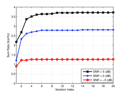
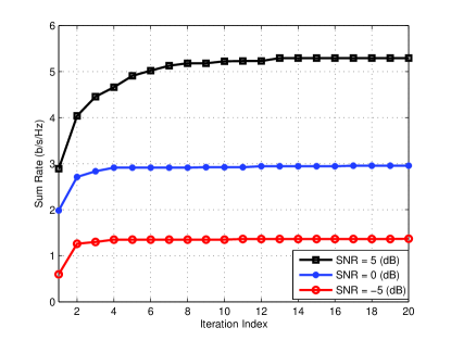
Figures 4 and 5 show the convergence behaviors of the proposed algorithm at different SNRs and under different modulations for the sum-rate (μ1=μ2=1subscript𝜇1subscript𝜇21\mu_{1}=\mu_{2}=1) maximization. For backtracking line search in Algorithm 1, the typical parameters are chosen as α=0.1𝛼0.1\alpha=0.1 and β=0.5𝛽0.5\beta=0.5 [33]. Statistical averages in (7) and (21) are evaluated via Monte Carlo drawings of 100010001000 random samples. These figures illustrate the evolutions of the sum-rate for each iterative step. We can see that in all the cases, the proposed algorithm converges within about 10 iteration steps.
Refer to caption
Figure 4: Convergence of sum rate maximization with BPSK modulation.
Refer to caption
Figure 5: Convergence of sum rate maximization with QPSK modulation.

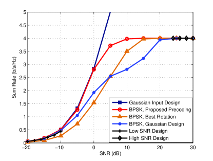
Figure 6 compares the sum-rate performances666It is noted that practical techniques can be employed in the random initial point selection process. For instance, the initial precoder at current SNR level can be generated by a weighted combination of the final precoder obtained at previous SNR level and a randomly generated precoder. Since the SNR step in our simulation is not large, this can take advantage of the previously computed precoder and accelerate the convergence speed. In general, for finite alphabet input signals, the WSR value lies in a limited bounded space. Therefore, 2-3 times random initializations are often sufficient to achieve a near-optimal WSR performance. of BPSK modulation under different transmit precoding schemes. We extend the idea for two-user SISO interference channels in [26] by a numerical search for the best rotation angle θ𝜃\theta for the second user constellation set ejθ𝐱2,j,j=1,2,,M2,θ[0,2π)formulae-sequencesuperscript𝑒𝑗𝜃subscript𝐱2𝑗𝑗12subscript𝑀2𝜃02𝜋e^{j\theta}{\bf{x}}_{2,j},j=1,2,\cdots,M_{2},\theta\in[0,2\pi), which is denoted as “BPSK, Best Rotation”. With respect to “BPSK, Gaussian Design”, we implement the Gaussian input assumption linear precoding design by the iterative algorithm in [15], and compute the finite alphabet rate of this precoding design in (7). The “Low SNR Design”, the “High SNR Design”, and the sum-rate achieved by Gaussian input assumption in [15] are also evaluated and plotted.
Refer to caption
Figure 6: Sum rate of 222-user MIMO interference channels with BPSK modulation.

From Figure 6, we have the following observations:

  • 1)

    The proposed precoding has BPSK system performance close to the sum-rate upper bound achieved by Gaussian inputs when SNR is below 00 dB.

  • 2)

    Our proposed precoding provides obvious sum rate gains over comparison schemes throughout the tested SNR region. At the sum-rate of 333 b/s/Hz, the proposed precoding is about 6.56.56.5 dB and 121212 dB better than the “BPSK, Best Rotation” and “BPSK, Gaussian Design”, respectively.

  • 3)

    The performances of the “Low SNR Design” and the sum-rate achieved by Gaussian inputs are virtually identical at low SNR.

  • 4)

    The sum-rate of the “High SNR Design” saturates at j=1Klog2Mj=4superscriptsubscript𝑗1𝐾subscript2subscript𝑀𝑗4\sum\nolimits_{j=1}^{K}\log_{2}{M_{j}}=4 b/s/Hz in high SNR region.

For BPSK modulation, the final precoding matrices obtained via Algorithm 1 when SNR=5SNR5{\rm{SNR}}=5 dB are given by

𝐆1=subscript𝐆1absent\displaystyle{\mathbf{G}}_{1}= [0.53900.7978j1.0204+0.1993j1.01660.1732j0.2907+0.0809j]delimited-[]0.53900.7978𝑗1.02040.1993𝑗1.01660.1732𝑗0.29070.0809𝑗\displaystyle\left[\begin{array}[]{lr}0.5390-0.7978j&1.0204+0.1993j\\ -1.0166-0.1732j&0.2907+0.0809j\\ \end{array}\right] (45)
𝐆2=subscript𝐆2absent\displaystyle{\mathbf{G}}_{2}= [0.0063+0.0404j0.28020.3445j1.2232+0.0059j0.63861.0292j].delimited-[]0.00630.0404𝑗0.28020.3445𝑗1.22320.0059𝑗0.63861.0292𝑗\displaystyle\left[\begin{array}[]{lr}-0.0063+0.0404j&0.2802-0.3445j\\ 1.2232+0.0059j&0.6386-1.0292j\\ \end{array}\right]. (48)

The sum-rate performances under different transmit precoding schemes with QPSK inputs are illustrated in Figure 7. We have similar observations with the BPSK case, where the proposed precoding achieves higher sum-rate than other precoding schemes, and the sum-rate performance of the “Low SNR Design” matches closely with the performance of the Gaussian input case in low SNR region. At a targeted sum-rate of 666 b/s/Hz, the performance gains of the proposed precoding over the “QPSK, Best Rotation” and “QPSK, Gaussian Design” are about 4.54.54.5 dB and777It should be noted that as the constellation size increases, the performance gap between the finite alphabet input design and the Gaussian input design will decrease. 101010 dB, respectively. Note that the sum-rate performances of the “High SNR Design” achieve j=1Klog2Mj=8superscriptsubscript𝑗1𝐾subscript2subscript𝑀𝑗8\sum\nolimits_{j=1}^{K}\log_{2}{M_{j}}=8 b/s/Hz in high SNR region. Furthermore, we observe that in both BPSK and QPSK cases, linear precoding design based on Gaussian input assumption performs almost identically as the proposed precoding in low SNR region, which corroborates the conclusion in Corollary 1.
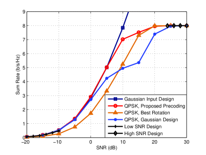
Refer to caption
Figure 7: Sum rate of 222-user MIMO interference channels with QPSK modulation.

For QPSK modulation, the final precoding matrices obtained via Algorithm 1 when SNR=5SNR5{\rm{SNR}}=5 dB are given by

𝐆1=subscript𝐆1absent\displaystyle{\mathbf{G}}_{1}= [1.05230.6658j0.23121.1369j0.37590.0377j0.20900.2814j]delimited-[]1.05230.6658𝑗0.23121.1369𝑗0.37590.0377𝑗0.20900.2814𝑗\displaystyle\left[\begin{array}[]{lr}1.0523-0.6658j&0.2312-1.1369j\\ 0.3759-0.0377j&0.2090-0.2814j\\ \end{array}\right] (51)
𝐆2=subscript𝐆2absent\displaystyle{\mathbf{G}}_{2}= [0.4825+0.0572j0.2828+0.1678j0.8290+1.0292j1.0257+0.1388j].delimited-[]0.48250.0572𝑗0.28280.1678𝑗0.82901.0292𝑗1.02570.1388𝑗\displaystyle\left[\begin{array}[]{lr}-0.4825+0.0572j&0.2828+0.1678j\\ -0.8290+1.0292j&1.0257+0.1388j\\ \end{array}\right]. (54)

As a more comprehensive comparison, we obtain the coded BER performances of a 2-user MIMO interference channel system illustrated in Figure 2 and 3. The LDPC encoder and decoder simulation package [38] is used, for coding rate 3/4343/4 and coding length L=9600𝐿9600L=9600. The MAP detector given in (29) is employed. The number of iterations between the MAP detector and the LDPC decoder is set to 5. Figure 8 plots the coded BER curves with different precoding schemes under BPSK modulation. We observe from Figure 8 that, at a targeted BER of 104superscript10410^{-4}, the corresponding SNR gains of the proposed precoding over “BPSK, Best Rotation” and “BPSK, Gaussian Design” schemes are about 777 dB and 13.513.513.5 dB, respectively. This suggests that the proposed precoding is very promising as it shows direct improvement on the coded BER performance in practical systems. Furthermore, comparing the performances of the proposed precoding and the Gaussian schemes in Figure 6 and Figure 8, we note that the SNR gains for the coded BER are larger than the corresponding SNR gains for the sum-rate shown in Figure 6. The reason for this observation is that we average the coded BER of 222 users to generate Figure 8. Therefore, the average coded BER is dominated by the user with larger coded BER.
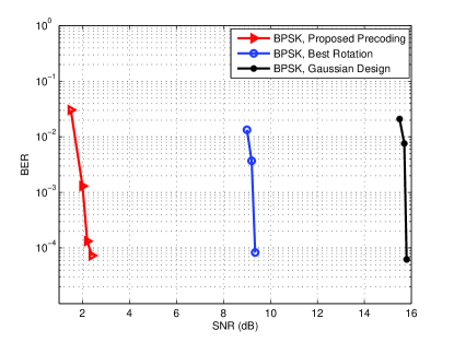
Refer to caption
Figure 8: BER of 222-user MIMO interference channels with BPSK modulation.

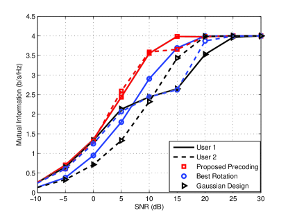
To confirm this, we present the mutual information of individual users under different precoding schemes and BPSK modulation in Figure 9. It is revealed in Figure 9 that, e.g., although the sum-rate is above 333 b/s/Hz for the Gaussian precoder design when SNR=14SNR14{\rm{SNR}}=14 dB, the achievable rate for user 1 is below 1.51.51.5 b/s/Hz. Therefore, the overall coded BER is still high for the Gaussian design in Figure 8 when SNR=14SNR14{\rm{SNR}}=14 dB. Also, we can observe from Figure 9 that the SNR gain for the user 1 of the proposed precoding over user 1 of the Gaussian design at rate 1.51.51.5 b/s/Hz is about 13.513.513.5 dB. The results correspond to the SNR gains for the coded BER in Figure 8.
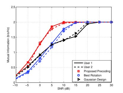
Refer to caption
Figure 9: Mutual information for individual user with BPSK modulation.

Figure 10 depicts the coded BER curves with QPSK inputs. The observations in Figure 10 are similar with the BPSK case. At a targeted coded BER of 104superscript10410^{-4}, the proposed precoding design has 5.55.55.5 dB and 101010 dB SNR gains over “QPSK, Best Rotation” and “QPSK, Gaussian Design”, respectively. Also, the coded BER results coincide with the mutual information results for individual users under QPSK modulation and different precoder designs as shown in Figure 11.
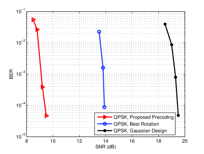
Refer to caption
Figure 10: BER of 222-user MIMO interference channels with QPSK modulation.
Refer to caption
Figure 11: Mutual information for individual user with QPSK modulation.

Next, the coded BER performances of using the detection method in (28) (denoted as “Gaussian Assumption Detection”) and the detection method in (29) (denoted as “Proposed Detection”) under different modulations are compared. Simulation results are listed in Table I. The precoders obtained via Algorithm 1 are used at the transmitter. From the results shown in Table I, it is seen that the “Proposed Detection” achieves lower BER than the “Gaussian Assumption Detection”, which indicates that exploiting the interference constellation structure can lead to additional performance gains in practical systems.

\captionstyle

center Modulation SNR (dB) Proposed Gaussian Detection Assumption Detection BPSK 2 0.0013 0.0114 2.5 0 7.513×1047.513superscript1047.513\times 10^{-4} 3 0 0 3.5 0 0 QPSK 9 0.0086 0.0780 10 0 0.0712 11 0 0.0578 12 0 0.0476
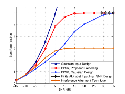
TABLE I: BER Results Using Different Detection Methods.
Refer to caption
Figure 12: Sum rate of 333-user MIMO interference channels with BPSK modulation.
Refer to caption
Figure 13: Sum rate of 333-user MIMO interference channels with QPSK modulation.

Finally, we further investigate the precoding design in a 333-user MIMO interference channel system. The channel matrices are given by

𝐇11=subscript𝐇11absent\displaystyle{\bf{H}}_{11}= (0.22790.6039j0.0660+0.6264j0.8774+0.6273j0.15150.0198j)0.22790.6039𝑗0.06600.6264𝑗0.87740.6273𝑗0.15150.0198𝑗\displaystyle\left(\begin{array}[]{lr}-0.2279-0.6039j&0.0660+0.6264j\\ -0.8774+0.6273j&0.1515-0.0198j\\ \end{array}\right) (57)
𝐇12=subscript𝐇12absent\displaystyle{\bf{H}}_{12}= (0.19150.3442j0.10920.0798j0.1022+1.2773j0.4246+0.0667j)0.19150.3442𝑗0.10920.0798𝑗0.10221.2773𝑗0.42460.0667𝑗\displaystyle\left(\begin{array}[]{lr}0.1915-0.3442j&-0.1092-0.0798j\\ 0.1022+1.2773j&0.4246+0.0667j\\ \end{array}\right) (60)
𝐇13=subscript𝐇13absent\displaystyle{\bf{H}}_{13}= (0.5759+0.1583j0.10920.0798j0.1022+1.2773j0.4246+0.0667j)0.57590.1583𝑗0.10920.0798𝑗0.10221.2773𝑗0.42460.0667𝑗\displaystyle\left(\begin{array}[]{lr}0.5759+0.1583j&-0.1092-0.0798j\\ 0.1022+1.2773j&0.4246+0.0667j\\ \end{array}\right) (63)
𝐇21=subscript𝐇21absent\displaystyle{\bf{H}}_{21}= (0.33820.7046j0.61310.1955j0.4195+0.2793j0.7792+0.3374j)0.33820.7046𝑗0.61310.1955𝑗0.41950.2793𝑗0.77920.3374𝑗\displaystyle\left(\begin{array}[]{lr}-0.3382-0.7046j&0.6131-0.1955j\\ 0.4195+0.2793j&-0.7792+0.3374j\\ \end{array}\right) (66)
𝐇22=subscript𝐇22absent\displaystyle{\bf{H}}_{22}= (0.4643+0.6778j0.73440.0113j0.40520.6845j0.38060.0892j)0.46430.6778𝑗0.73440.0113𝑗0.40520.6845𝑗0.38060.0892𝑗\displaystyle\left(\begin{array}[]{lr}0.4643+0.6778j&0.7344-0.0113j\\ 0.4052-0.6845j&0.3806-0.0892j\\ \end{array}\right) (69)
𝐇23=subscript𝐇23absent\displaystyle{\bf{H}}_{23}= (0.82380.4134j0.5425+0.1126j0.1321+0.2715j0.72670.4734j)0.82380.4134𝑗0.54250.1126𝑗0.13210.2715𝑗0.72670.4734𝑗\displaystyle\left(\begin{array}[]{lr}-0.8238-0.4134j&0.5425+0.1126j\\ 0.1321+0.2715j&0.7267-0.4734j\\ \end{array}\right) (72)
𝐇31=subscript𝐇31absent\displaystyle{\bf{H}}_{31}= (0.9707+0.2271j0.45200.2644j0.02650.7569j0.27480.2878j)0.97070.2271𝑗0.45200.2644𝑗0.02650.7569𝑗0.27480.2878𝑗\displaystyle\left(\begin{array}[]{lr}-0.9707+0.2271j&-0.4520-0.2644j\\ -0.0265-0.7569j&0.2748-0.2878j\\ \end{array}\right) (75)
𝐇32=subscript𝐇32absent\displaystyle{\bf{H}}_{32}= (0.22000.0000j0.0113+0.6334j0.58370.1839j0.02791.0840j)0.22000.0000𝑗0.01130.6334𝑗0.58370.1839𝑗0.02791.0840𝑗\displaystyle\left(\begin{array}[]{lr}-0.2200-0.0000j&-0.0113+0.6334j\\ -0.5837-0.1839j&-0.0279-1.0840j\\ \end{array}\right) (78)
𝐇33=subscript𝐇33absent\displaystyle{\bf{H}}_{33}= (0.22000.0000j0.0113+0.6334j0.58370.1839j0.02791.0840j).0.22000.0000𝑗0.01130.6334𝑗0.58370.1839𝑗0.02791.0840𝑗\displaystyle\left(\begin{array}[]{lr}-0.2200-0.0000j&-0.0113+0.6334j\\ -0.5837-0.1839j&-0.0279-1.0840j\\ \end{array}\right). (81)

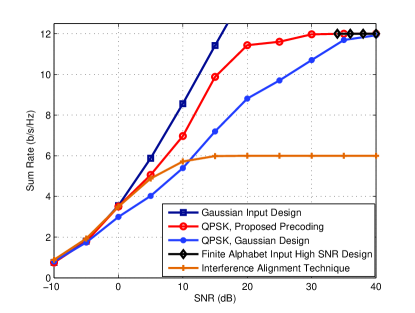
Figure 12 compares the sum-rate performances of different precoding designs with BPSK inputs. The sum-rates achieved by the proposed “Finite Alphabet Input High SNR Design” and the “Interference Alignment Technique” are also plotted. It is observed from Figure 12 that the proposed precoding outperforms other precoding designs. At a targeted sum-rate of 4.54.54.5 b/s/Hz, our proposed precoding has about 101010 dB SNR gains over the Gaussian design. Moreover, the sum-rate performances with QPSK inputs are plotted in Figure 13. At a targeted sum-rate of 999 b/s/Hz, the performance gains of the proposed precoding over the Gaussian design are about 888 dB. We note that, in both modulations, the sum-rates achieved by the “Finite Alphabet Input High SNR Design” saturate at Rsum=j=1Klog2Mjsuperscriptsubscript𝑅sumsuperscriptsubscript𝑗1𝐾subscript2subscript𝑀𝑗R_{\rm{sum}}^{\infty}=\sum\nolimits_{j=1}^{K}{\log_{2}M_{j}} b/s/Hz, and the “Interference Alignment” has 50%percent5050\% sum-rate losses888It is noted that each user transmits one data stream for the IA method. Although the IA approach can align other users’ interference into a signal space and eliminate them, it is still suboptimal. This is because the mutual information with finite alphabet inputs is bounded. Thus, allocating more power to the already saturated signals can not further improve the mutual information. This implies that transmitting only one data stream for each user will result in a constant sum-rate loss in finite alphabet input scenarios. Instead, for the proposed method in Algorithm 1 and the high SNR design in Proposition 3, each user transmits two data streams. It is shown in Figure 12 and Figure 13 that both Algorithm 1 and the proposed high SNR design in Proposition 3 can effectively combat interference and achieve the saturated sum-rate j=1Klog2Mjsuperscriptsubscript𝑗1𝐾subscript2subscript𝑀𝑗\sum\nolimits_{j=1}^{K}{\log_{2}M_{j}} b/s/Hz at high SNR. as implied in Corollary 2.

V Conclusion

This work investigated the linear precoding design for MIMO interference channel systems. To break away from the traditional studies based on Gaussian input assumption, we formulated the problem of maximizing mutual information for finite alphabet inputs. We derived the achievable rate expression of each user. Our analysis at the high SNR revealed that the IA technique designed for Gaussian input case will lead to a significant sum-rate loss due to the utilization of partial interference-free signal space for transmission. In light of this, we developed an efficient power allocation scheme designed for finite alphabet input scenario at high SNR. The proposed scheme achieves the analytical upper-bound sum-rate of the entire signal space j=1Klog2Mjsuperscriptsubscript𝑗1𝐾subscript2subscript𝑀𝑗\sum\nolimits_{j=1}^{K}{\log_{2}M_{j}} b/s/Hz under finite alphabet constraints. More generally, we derived a set of necessary conditions for the WSR maximization precoding design based on Karush-Kuhn-Tucker (KKT) analysis, from which we developed an iterative algorithm for precoding optimization. We applied gradient descent optimization and used backtracking line search algorithm to regulate the convergence speed. Our tests, based on LDPC coded QAM signals in the MIMO interference channels established the coded BER performance gain of the obtained linear precoders.

Acknowledgment

The authors would like to thank the editor, Prof. Tony Q. S. Quek, and anonymous reviewers for helpful comments and suggestions that greatly improved the quality of the paper.

Appendix A Proof of Proposition 1

When the discrete input data vector 𝐱ksubscript𝐱𝑘{\mathbf{x}}_{k} is independent and uniformly distributed from the constellation set Sjsubscript𝑆𝑗S_{j}, the a priori probabilities of 𝐱j,psubscript𝐱𝑗𝑝{\mathbf{x}}_{j,p} is p(𝐱j=𝐱j,p)=1Mj𝑝subscript𝐱𝑗subscript𝐱𝑗𝑝1subscript𝑀𝑗p({\mathbf{x}}_{j}={\mathbf{x}}_{j,p})=\frac{1}{{M_{j}}}, p=1,2,,Mj𝑝12subscript𝑀𝑗p=1,2,\cdots,M_{j}, j=1,2,,K𝑗12𝐾j=1,2,\cdots,K. Then, according to the definition of conditional entropy [39] and the Bayes’ theorem, we can evaluate H(𝐲j)𝐻subscript𝐲𝑗H\left({{\bf{y}}_{j}}\right) and H(𝐲j|𝐱j)𝐻conditionalsubscript𝐲𝑗subscript𝐱𝑗H\left({{\bf{y}}_{j}\left|{{\bf{x}}_{j}}\right.}\right) given in (82) and (83) at the top of the next page.

H(𝐲j)=i=1Klog2Mi+1i=1KMim1=1M1m2=1M2mK=1MKp(𝐲j|𝐱1,m1,𝐱2,m2,,𝐱K,mK)×log21n1=1M1n2=1M2nK=1MKp(𝐲j|𝐱1,n1,𝐱2,n2,,𝐱K,nK)d𝐲j𝐻subscript𝐲𝑗superscriptsubscript𝑖1𝐾subscript2subscript𝑀𝑖1superscriptsubscriptproduct𝑖1𝐾subscript𝑀𝑖superscriptsubscriptsubscript𝑚11subscript𝑀1superscriptsubscriptsubscript𝑚21subscript𝑀2superscriptsubscriptsubscript𝑚𝐾1subscript𝑀𝐾𝑝conditionalsubscript𝐲𝑗subscript𝐱1subscript𝑚1subscript𝐱2subscript𝑚2subscript𝐱𝐾subscript𝑚𝐾absentsubscript21superscriptsubscriptsubscript𝑛11subscript𝑀1superscriptsubscriptsubscript𝑛21subscript𝑀2superscriptsubscriptsubscript𝑛𝐾1subscript𝑀𝐾𝑝conditionalsubscript𝐲𝑗subscript𝐱1subscript𝑛1subscript𝐱2subscript𝑛2subscript𝐱𝐾subscript𝑛𝐾𝑑subscript𝐲𝑗\begin{array}[]{l}H\left({{\bf{y}}_{j}}\right)=\sum\limits_{i=1}^{K}{\log_{2}M_{i}+\frac{1}{{\prod\nolimits_{i=1}^{K}{M_{i}}}}}\sum\limits_{m_{1}=1}^{M_{1}}\sum\limits_{m_{2}=1}^{M_{2}}\cdots{\sum\limits_{m_{K}=1}^{M_{K}}{{\scalebox{1.0}[1.2]{$\int$}}{p\left({{\bf{y}}_{j}\left|{{\bf{x}}_{1,m_{1}},{\bf{x}}_{2,m_{2}},\cdots,{\bf{x}}_{K,m_{K}}}\right.}\right)}}}\\ \qquad\qquad\qquad\qquad\times\log_{2}\frac{1}{{\sum\limits_{n_{1}=1}^{M_{1}}\sum\limits_{n_{2}=1}^{M_{2}}{\cdots\sum\limits_{n_{K}=1}^{M_{K}}{p\left({{\bf{y}}_{j}\left|{{\bf{x}}_{1,n_{1}},{\bf{x}}_{2,n_{2}},\cdots,{\bf{x}}_{K,n_{K}}}\right.}\right)}}}}d{\bf{y}}_{j}\\ \end{array} (82)
H(𝐲j|𝐱j)=i=1,ijKMi+1i=1KMim1=1M1m2=1M2mK=1MKp(𝐲j|𝐱1,m1,𝐱2,m2,,𝐱K,mK)×log21n1=1M1nj1=1Mj1nj+1=1Mj+1nK=1MKp(𝐲j|𝐱j,mj,𝐱1,n1,,𝐱j1,nk1,𝐱j+1,nj+1,,𝐱K,nK)d𝐲j.𝐻conditionalsubscript𝐲𝑗subscript𝐱𝑗superscriptsubscriptformulae-sequence𝑖1𝑖𝑗𝐾subscript𝑀𝑖1superscriptsubscriptproduct𝑖1𝐾subscript𝑀𝑖superscriptsubscriptsubscript𝑚11subscript𝑀1superscriptsubscriptsubscript𝑚21subscript𝑀2superscriptsubscriptsubscript𝑚𝐾1subscript𝑀𝐾𝑝conditionalsubscript𝐲𝑗subscript𝐱1subscript𝑚1subscript𝐱2subscript𝑚2subscript𝐱𝐾subscript𝑚𝐾absentsubscript21superscriptsubscriptsubscript𝑛11subscript𝑀1superscriptsubscriptsubscript𝑛𝑗11subscript𝑀𝑗1superscriptsubscriptsubscript𝑛𝑗11subscript𝑀𝑗1superscriptsubscriptsubscript𝑛𝐾1subscript𝑀𝐾𝑝conditionalsubscript𝐲𝑗subscript𝐱𝑗subscript𝑚𝑗subscript𝐱1subscript𝑛1subscript𝐱𝑗1subscript𝑛𝑘1subscript𝐱𝑗1subscript𝑛𝑗1subscript𝐱𝐾subscript𝑛𝐾𝑑subscript𝐲𝑗\begin{array}[]{l}H\left({{\bf{y}}_{j}\left|{{\bf{x}}_{j}}\right.}\right)=\sum\limits_{i=1,i\neq j}^{K}{M_{i}}+\frac{1}{{\prod\nolimits_{i=1}^{K}{M_{i}}}}\sum\limits_{m_{1}=1}^{M_{1}}\sum\limits_{m_{2}=1}^{M_{2}}\cdots{\sum\limits_{m_{K}=1}^{M_{K}}{{\scalebox{1.0}[1.5]{$\int$}}{p\left({{\bf{y}}_{j}\left|{{\bf{x}}_{1,m_{1}},{\bf{x}}_{2,m_{2}},\cdots,{\bf{x}}_{K,m_{K}}}\right.}\right)}}}\\ \qquad\qquad\qquad\qquad\times\log_{2}\frac{1}{{\sum\limits_{n_{1}=1}^{M_{1}}{\cdots\sum\limits_{n_{j-1}=1}^{M_{j-1}}{\sum\limits_{n_{j+1}=1}^{M_{j+1}}{\cdots\sum\limits_{n_{K}=1}^{M_{K}}{p\left({{\bf{y}}_{j}\left|{{\bf{x}}_{j,m_{j}},{\bf{x}}_{1,n_{1}},\cdots,{\bf{x}}_{j-1,n_{k-1}},{\bf{x}}_{j+1,n_{j+1}},...,{\bf{x}}_{K,n_{K}}}\right.}\right)}}}}}}d{\bf{y}}_{j}.\\ \end{array} (83)

From model (1), we have

p(𝐲j|𝐱1,m1,𝐱2,m2,,𝐱K,mK)=1(πσ2)Nrjexp(𝐲ji=1K𝐇ji𝐆i𝐱i.mi2σ2)𝑝conditionalsubscript𝐲𝑗subscript𝐱1subscript𝑚1subscript𝐱2subscript𝑚2subscript𝐱𝐾subscript𝑚𝐾absent1superscript𝜋superscript𝜎2subscript𝑁subscript𝑟𝑗superscriptnormsubscript𝐲𝑗superscriptsubscript𝑖1𝐾subscript𝐇𝑗𝑖subscript𝐆𝑖subscript𝐱formulae-sequence𝑖subscript𝑚𝑖2superscript𝜎2\begin{array}[]{l}p\left({{\bf{y}}_{j}\left|{{\bf{x}}_{1,m_{1}},{\bf{x}}_{2,m_{2}},\cdots,{\bf{x}}_{K,m_{K}}}\right.}\right)\\ \qquad\qquad\qquad=\frac{1}{{\left({\pi{\displaystyle\sigma}^{2}}\right)^{N_{r_{j}}}}}\exp\left({-\frac{{\left\|{{\bf{y}}_{j}-\sum\limits_{i=1}^{K}{{\bf{H}}_{ji}{\bf{G}}_{i}{\bf{x}}_{i.m_{i}}}}\right\|^{2}}}{{{\displaystyle\sigma}^{2}}}}\right)\end{array} (84)
p(𝐲j|𝐱1,n1,𝐱2,n2,,𝐱K,nK)=1(πσ2)Nrjexp(𝐲ji=1K𝐇ji𝐆i𝐱i.ni2σ2)𝑝conditionalsubscript𝐲𝑗subscript𝐱1subscript𝑛1subscript𝐱2subscript𝑛2subscript𝐱𝐾subscript𝑛𝐾absent1superscript𝜋superscript𝜎2subscript𝑁subscript𝑟𝑗superscriptnormsubscript𝐲𝑗superscriptsubscript𝑖1𝐾subscript𝐇𝑗𝑖subscript𝐆𝑖subscript𝐱formulae-sequence𝑖subscript𝑛𝑖2superscript𝜎2\begin{array}[]{l}p\left({{\bf{y}}_{j}\left|{{\bf{x}}_{1,n_{1}},{\bf{x}}_{2,n_{2}},\cdots,{\bf{x}}_{K,n_{K}}}\right.}\right)\\ \qquad\qquad\qquad=\frac{1}{{\left({\pi{\displaystyle\sigma}^{2}}\right)^{N_{r_{j}}}}}\exp\left({-\frac{{\left\|{{\bf{y}}_{j}-\sum\limits_{i=1}^{K}{{\bf{H}}_{ji}{\bf{G}}_{i}{\bf{x}}_{i.n_{i}}}}\right\|^{2}}}{{{\displaystyle\sigma}^{2}}}}\right)\end{array} (85)
p(𝐲j|𝐱j,mj,𝐱1,n1,,𝐱j1,nj1,𝐱j+1,nj+1,,𝐱K,nK)=1(πσ2)Nrjexp(𝐲j𝐇jj𝐆j𝐱j.mji=1,ijK𝐇ji𝐆i𝐱i.ni2σ2).𝑝conditionalsubscript𝐲𝑗subscript𝐱𝑗subscript𝑚𝑗subscript𝐱1subscript𝑛1subscript𝐱𝑗1subscript𝑛𝑗1subscript𝐱𝑗1subscript𝑛𝑗1subscript𝐱𝐾subscript𝑛𝐾absent1superscript𝜋superscript𝜎2subscript𝑁subscript𝑟𝑗superscriptnormsubscript𝐲𝑗subscript𝐇𝑗𝑗subscript𝐆𝑗subscript𝐱formulae-sequence𝑗subscript𝑚𝑗superscriptsubscriptformulae-sequence𝑖1𝑖𝑗𝐾subscript𝐇𝑗𝑖subscript𝐆𝑖subscript𝐱formulae-sequence𝑖subscript𝑛𝑖2superscript𝜎2\begin{array}[]{l}p\left({{\bf{y}}_{j}\left|{{\bf{x}}_{j,m_{j}},{\bf{x}}_{1,n_{1}},\cdots,{\bf{x}}_{j-1,n_{j-1}},{\bf{x}}_{j+1,n_{j+1}},\cdots,{\bf{x}}_{K,n_{K}}}\right.}\right)\\ =\frac{1}{{\left({\pi{\displaystyle\sigma}^{2}}\right)^{N_{r_{j}}}}}\exp\left({-\frac{{\left\|{{\bf{y}}_{j}-{\bf{H}}_{jj}{\bf{G}}_{j}{\bf{x}}_{j.m_{j}}-\sum\limits_{i=1,i\neq j}^{K}{{\bf{H}}_{ji}{\bf{G}}_{i}{\bf{x}}_{i.n_{i}}}}\right\|^{2}}}{{{\displaystyle\sigma}^{2}}}}\right).\\ \end{array} (86)

Plugging (84)–(86) into (82) and (83) and define 𝐧=𝐲ji=1K𝐇ji𝐆i𝐱i,mi𝐧subscript𝐲𝑗superscriptsubscript𝑖1𝐾subscript𝐇𝑗𝑖subscript𝐆𝑖subscript𝐱𝑖subscript𝑚𝑖{\mathbf{n}}={\mathbf{y}}_{j}-\sum\nolimits_{i=1}^{K}{{\bf{H}}_{ji}{\bf{G}}_{i}{\bf{x}}_{i,m_{i}}}, yields

H(𝐲j)=i=1Klog2Mi1i=1KMim1=1M1m2=1M2mK=1MKp(𝐧)log2H1,j(m1,m2,,mK,𝐧)𝑑𝐧𝐻subscript𝐲𝑗superscriptsubscript𝑖1𝐾subscript2subscript𝑀𝑖1superscriptsubscriptproduct𝑖1𝐾subscript𝑀𝑖superscriptsubscriptsubscript𝑚11subscript𝑀1superscriptsubscriptsubscript𝑚21subscript𝑀2superscriptsubscriptsubscript𝑚𝐾1subscript𝑀𝐾𝑝𝐧subscript2subscript𝐻1𝑗subscript𝑚1subscript𝑚2subscript𝑚𝐾𝐧differential-d𝐧\begin{array}[]{l}H\left({{\bf{y}}_{j}}\right)=\sum\limits_{i=1}^{K}{\log_{2}M_{i}}-\frac{1}{{\prod\nolimits_{i=1}^{K}{M_{i}}}}\sum\limits_{m_{1}=1}^{M_{1}}\sum\limits_{m_{2}=1}^{M_{2}}\cdots\\ \qquad\qquad\sum\limits_{m_{K}=1}^{M_{K}}{\int{p\left({\bf{n}}\right)\log_{2}H_{1,j}\left({m_{1},m_{2},\cdots,m_{K},{\mathbf{n}}}\right)}}d{\bf{n}}\end{array} (87)
=i=1Klog2Mi1i=1KMim1=1M1m2=1M2mK=1MKE𝐧[log2H1,j(m1,m2,,mK,𝐧)]absentsuperscriptsubscript𝑖1𝐾subscript2subscript𝑀𝑖1superscriptsubscriptproduct𝑖1𝐾subscript𝑀𝑖superscriptsubscriptsubscript𝑚11subscript𝑀1superscriptsubscriptsubscript𝑚21subscript𝑀2superscriptsubscriptsubscript𝑚𝐾1subscript𝑀𝐾subscript𝐸𝐧delimited-[]subscript2subscript𝐻1𝑗subscript𝑚1subscript𝑚2subscript𝑚𝐾𝐧\begin{array}[]{l}\qquad\ \ =\sum\limits_{i=1}^{K}{\log_{2}M_{i}}-\frac{1}{{\prod\nolimits_{i=1}^{K}{M_{i}}}}\sum\limits_{m_{1}=1}^{M_{1}}\sum\limits_{m_{2}=1}^{M_{2}}\cdots\\ \qquad\qquad\quad\sum\limits_{m_{K}=1}^{M_{K}}{E_{\bf{n}}\left[{\log_{2}H_{1,j}\left({m_{1},m_{2},\cdots,m_{K},{\mathbf{n}}}\right)}\right]}\end{array} (88)
H(𝐲j|𝐱j)=i=1,ijKlog2Mi1i=1KMim1=1M1m2=1M2mK=1MKp(𝐧)log2H2,j(m1,,mj1,mj+1,,mK,𝐧)𝑑𝐧𝐻conditionalsubscript𝐲𝑗subscript𝐱𝑗superscriptsubscriptformulae-sequence𝑖1𝑖𝑗𝐾subscript2subscript𝑀𝑖1superscriptsubscriptproduct𝑖1𝐾subscript𝑀𝑖superscriptsubscriptsubscript𝑚11subscript𝑀1superscriptsubscriptsubscript𝑚21subscript𝑀2superscriptsubscriptsubscript𝑚𝐾1subscript𝑀𝐾𝑝𝐧subscript2subscript𝐻2𝑗subscript𝑚1subscript𝑚𝑗1subscript𝑚𝑗1subscript𝑚𝐾𝐧differential-d𝐧\begin{array}[]{l}H\left({{\bf{y}}_{j}\left|{{\bf{x}}_{j}}\right.}\right)=\!\!\sum\limits_{i=1,i\neq j}^{K}{\log_{2}M_{i}}-\frac{1}{{\prod\nolimits_{i=1}^{K}{M_{i}}}}\sum\limits_{m_{1}=1}^{M_{1}}\sum\limits_{m_{2}=1}^{M_{2}}\!\cdots\!\\ \sum\limits_{m_{K}=1}^{M_{K}}\int p\left({\bf{n}}\right)\log_{2}H_{2,j}\left({m_{1},\!\cdots\!,m_{j-1},m_{j+1},\!\cdots\!,m_{K},{\mathbf{n}}}\right)d{\bf{n}}\end{array} (89)
=i=1,ijKlog2Mi1i=1KMim1=1M1m2=1M2mK=1MKE𝐧[log2H2,j(m1,,mj1,mj+1,,mK,𝐧)].absentsuperscriptsubscriptformulae-sequence𝑖1𝑖𝑗𝐾subscript2subscript𝑀𝑖1superscriptsubscriptproduct𝑖1𝐾subscript𝑀𝑖superscriptsubscriptsubscript𝑚11subscript𝑀1superscriptsubscriptsubscript𝑚21subscript𝑀2superscriptsubscriptsubscript𝑚𝐾1subscript𝑀𝐾subscript𝐸𝐧delimited-[]subscript2subscript𝐻2𝑗subscript𝑚1subscript𝑚𝑗1subscript𝑚𝑗1subscript𝑚𝐾𝐧\begin{array}[]{l}\qquad\qquad\ =\sum\limits_{i=1,i\neq j}^{K}{\log_{2}M_{i}}-\frac{1}{{\prod\nolimits_{i=1}^{K}{M_{i}}}}\sum\limits_{m_{1}=1}^{M_{1}}\sum\limits_{m_{2}=1}^{M_{2}}\cdots\\ {\sum\limits_{m_{K}=1}^{M_{K}}{E_{\bf{n}}\left[{\log_{2}H_{2,j}\left({m_{1},\cdots,m_{j-1},m_{j+1},\cdots,m_{K},{\mathbf{n}}}\right)}\right]}}.\end{array} (90)

Then, the proposition is proved by utilizing the definition of the mutual information [39] Rj=I(𝐲j,𝐱j)=H(𝐲j)H(𝐲j|𝐱j)subscript𝑅𝑗𝐼subscript𝐲𝑗subscript𝐱𝑗𝐻subscript𝐲𝑗𝐻conditionalsubscript𝐲𝑗subscript𝐱𝑗R_{j}=I({\mathbf{y}}_{j},{\mathbf{x}}_{j})=H(\mathbf{y}_{j})-H\left({{\bf{y}}_{j}\left|{{\bf{x}}_{j}}\right.}\right), along with the expressions in (88) and (90).

Appendix B Proof of Proposition 2

First, we apply Jensen’s inequality [33] to obtain an approximation of (7) as follows

Rj,finitelogMj1i=1KMi×\displaystyle R_{{{j}},{\rm{finite}}}\approx\log M_{j}-\frac{1}{{\prod\nolimits_{i=1}^{K}{M_{i}}}}\times
[f1(E𝐧exp(1σ2(i=1K𝐇ji𝐆i(𝐱i,mi𝐱i,ni))+𝐧2))\displaystyle\left[\!f_{\rm{1}}\left(\!\!E_{\bf{n}}{\exp\left({\!-\!\frac{1}{{{\displaystyle\sigma}^{2}}}\left\|{\left(\!{\sum\limits_{i=1}^{K}{{\bf{H}}_{ji}{\bf{G}}_{i}\left({{\bf{x}}_{i,m_{i}}\!\!-\!\!{\bf{x}}_{i,n_{i}}}\right)}}\!\right)\!\!+\!\!{\bf{n}}}\right\|^{2}}\right)}\!\right)\right.-
f2(E𝐧exp(1σ2(i=1,ijK𝐇ji𝐆i(𝐱i,mi𝐱i,ni))+𝐧2))]\displaystyle\left.f_{\rm{2}}\!\!\left(\!\!{E_{\bf{n}}{\exp\left({\!\!-\frac{1}{{{\displaystyle\sigma}^{2}}}\left\|{\left({\sum\limits_{i=1,i\neq j}^{K}{{\bf{H}}_{ji}{\bf{G}}_{i}\left({{\bf{x}}_{i,m_{i}}\!\!-\!\!{\bf{x}}_{i,n_{i}}}\right)}}\right)\!\!+\!\!{\bf{n}}}\right\|^{2}}\right)}}\!\!\right)\!\!\right]

where we define the operations f1()subscript𝑓1f_{1}(\cdot), f2()subscript𝑓2f_{2}(\cdot), f3()subscript𝑓3f_{3}(\cdot) and f4()subscript𝑓4f_{4}(\cdot) as

f1()m1=1M1m2=1M2mK=1MKlog2n1=1M1n2=1M2nK=1MK()approaches-limitsubscript𝑓1superscriptsubscriptsubscript𝑚11subscript𝑀1superscriptsubscriptsubscript𝑚21subscript𝑀2superscriptsubscriptsubscript𝑚𝐾1subscript𝑀𝐾subscript2superscriptsubscriptsubscript𝑛11subscript𝑀1superscriptsubscriptsubscript𝑛21subscript𝑀2superscriptsubscriptsubscript𝑛𝐾1subscript𝑀𝐾f_{1}(\cdot)\doteq\sum\limits_{m_{1}=1}^{M_{1}}\sum\limits_{m_{2}=1}^{M_{2}}{\!\!\cdots\!\!\sum\limits_{m_{K}=1}^{M_{K}}{\log_{2}}}\sum\limits_{n_{1}=1}^{M_{1}}\sum\limits_{n_{2}=1}^{M_{2}}{\!\!\cdots\!\!\sum\limits_{n_{K}=1}^{M_{K}}}(\cdot) (92)
f2()m1=1M1m2=1M2mK=1MKlog2n1=1M1nj1=1Mj1nj+1=1Mj+1nK=1MK()approaches-limitsubscript𝑓2superscriptsubscriptsubscript𝑚11subscript𝑀1superscriptsubscriptsubscript𝑚21subscript𝑀2superscriptsubscriptsubscript𝑚𝐾1subscript𝑀𝐾subscript2superscriptsubscriptsubscript𝑛11subscript𝑀1superscriptsubscriptsubscript𝑛𝑗11subscript𝑀𝑗1superscriptsubscriptsubscript𝑛𝑗11subscript𝑀𝑗1superscriptsubscriptsubscript𝑛𝐾1subscript𝑀𝐾f_{2}(\cdot)\doteq\sum\limits_{m_{1}=1}^{M_{1}}\sum\limits_{m_{2}=1}^{M_{2}}\!\!\cdots\!\!\sum\limits_{m_{K}=1}^{M_{K}}\!{\log_{2}}\!\sum\limits_{n_{1}=1}^{M_{1}}\!\!\cdots\!\!\sum\limits_{n_{j-1}=1}^{M_{j-1}}\sum\limits_{n_{j+1}=1}^{M_{j+1}}\!\!\cdots\!\!\sum\limits_{n_{K}=1}^{M_{K}}(\cdot) (93)
f3()m1=1M1m2=1M2mK=1MKn1=1M1n2=1M2nK=1MK()approaches-limitsubscript𝑓3superscriptsubscriptsubscript𝑚11subscript𝑀1superscriptsubscriptsubscript𝑚21subscript𝑀2superscriptsubscriptsubscript𝑚𝐾1subscript𝑀𝐾superscriptsubscriptsubscript𝑛11subscript𝑀1superscriptsubscriptsubscript𝑛21subscript𝑀2superscriptsubscriptsubscript𝑛𝐾1subscript𝑀𝐾f_{3}(\cdot)\doteq\sum\limits_{m_{1}=1}^{M_{1}}\sum\limits_{m_{2}=1}^{M_{2}}{\!\!\cdots\!\!\sum\limits_{m_{K}=1}^{M_{K}}}\sum\limits_{n_{1}=1}^{M_{1}}\sum\limits_{n_{2}=1}^{M_{2}}{\!\!\cdots\!\!\sum\limits_{n_{K}=1}^{M_{K}}}(\cdot) (94)
f4()m1=1M1m2=1M2mK=1MKn1=1M1nj1=1Mj1nj+1=1Mj+1nK=1MK().approaches-limitsubscript𝑓4superscriptsubscriptsubscript𝑚11subscript𝑀1superscriptsubscriptsubscript𝑚21subscript𝑀2superscriptsubscriptsubscript𝑚𝐾1subscript𝑀𝐾superscriptsubscriptsubscript𝑛11subscript𝑀1superscriptsubscriptsubscript𝑛𝑗11subscript𝑀𝑗1superscriptsubscriptsubscript𝑛𝑗11subscript𝑀𝑗1superscriptsubscriptsubscript𝑛𝐾1subscript𝑀𝐾f_{4}(\cdot)\doteq\sum\limits_{m_{1}=1}^{M_{1}}\sum\limits_{m_{2}=1}^{M_{2}}\!\!\cdots\!\!\sum\limits_{m_{K}=1}^{M_{K}}\!\!\sum\limits_{n_{1}=1}^{M_{1}}\!\!\cdots\!\!\sum\limits_{n_{j-1}=1}^{M_{j-1}}\sum\limits_{n_{j+1}=1}^{M_{j+1}}\!\!\cdots\!\!\sum\limits_{n_{K}=1}^{M_{K}}(\cdot). (95)

Recalling the definition of 𝐧𝐧{\bf{n}} in (7), the first expectation in (B) can be evaluated as

E𝐧exp(1σ2(i=1K𝐇ji𝐆i(𝐱i,mi𝐱i,ni))+𝐧2)=𝐧exp(1σ2(i=1K𝐇ji𝐆i(𝐱i,mi𝐱i,ni))+𝐧2)subscript𝐸𝐧1superscript𝜎2superscriptnormsuperscriptsubscript𝑖1𝐾subscript𝐇𝑗𝑖subscript𝐆𝑖subscript𝐱𝑖subscript𝑚𝑖subscript𝐱𝑖subscript𝑛𝑖𝐧2absentsubscript𝐧1superscript𝜎2superscriptnormsuperscriptsubscript𝑖1𝐾subscript𝐇𝑗𝑖subscript𝐆𝑖subscript𝐱𝑖subscript𝑚𝑖subscript𝐱𝑖subscript𝑛𝑖𝐧2\begin{array}[]{l}E_{\bf{n}}\exp\left({-\frac{1}{{{\displaystyle\sigma}^{2}}}\left\|{\left({\sum\limits_{i=1}^{K}{{\bf{H}}_{ji}{\bf{G}}_{i}\left({{\bf{x}}_{i,m_{i}}-{\bf{x}}_{i,n_{i}}}\right)}}\right)+{\bf{n}}}\right\|^{2}}\right)\\ =\int_{\bf{n}}\exp\left({-\frac{1}{{{\displaystyle\sigma}^{2}}}\left\|{\left({\sum\limits_{i=1}^{K}{{\bf{H}}_{ji}{\bf{G}}_{i}\left({{\bf{x}}_{i,m_{i}}-{\bf{x}}_{i,n_{i}}}\right)}}\right)+{\bf{n}}}\right\|^{2}}\right)\\ \end{array}
×exp(𝐧2σ2)d𝐧×(πσ2)Nrabsentsuperscriptnorm𝐧2superscript𝜎2𝑑𝐧superscript𝜋superscript𝜎2subscript𝑁𝑟\begin{array}[]{l}\times\exp\left({-\frac{{\left\|{\bf{n}}\right\|^{2}}}{{{\displaystyle\sigma}^{2}}}}\right)d{\bf{n}}\times\left({\pi\sigma^{2}}\right)^{-N_{r}}\end{array}\\ (96)
=2Nrexp(12σ2(i=1K𝐇ji𝐆i(𝐱i,mi𝐱i,ni))2)×𝐧I1(𝐧)d𝐧\begin{array}[]{l}=2^{-N_{r}}\exp\left({-\frac{1}{{2\sigma^{2}}}\left\|{\left({\sum\limits_{i=1}^{K}{{\bf{H}}_{ji}{\bf{G}}_{i}\left({{\bf{x}}_{i,m_{i}}-{\bf{x}}_{i,n_{i}}}\right)}}\right)}\right\|^{2}}\right)\\ \qquad\qquad\qquad\qquad\qquad\qquad\times\int_{\bf{n}}{I_{1}\left({\bf{n}}\right)d{\bf{n}}}\\ \end{array} (97)

where

I1(𝐧)=(πσ22)Nr×\displaystyle\hskip 42.67912ptI_{1}\left({\bf{n}}\right)=\left({\frac{{\pi\sigma^{2}}}{2}}\right)^{-N_{r}}\times
exp(2σ2(12i=1K𝐇ji𝐆i(𝐱i,mi𝐱i,ni))+𝐧2)2superscript𝜎2superscriptnorm12superscriptsubscript𝑖1𝐾subscript𝐇𝑗𝑖subscript𝐆𝑖subscript𝐱𝑖subscript𝑚𝑖subscript𝐱𝑖subscript𝑛𝑖𝐧2\displaystyle\exp\left({-\frac{2}{{\sigma^{2}}}\left\|{\left({\frac{1}{2}\sum\limits_{i=1}^{K}{{\bf{H}}_{ji}{\bf{G}}_{i}\left({{\bf{x}}_{i,m_{i}}-{\bf{x}}_{i,n_{i}}}\right)}}\right)+{\bf{n}}}\right\|^{2}}\right) (98)

denotes a probability density function of an independent and identically distributed Gaussian vector with mean 12i=1K𝐇ji𝐆i(𝐱i,mi𝐱i,ni)12superscriptsubscript𝑖1𝐾subscript𝐇𝑗𝑖subscript𝐆𝑖subscript𝐱𝑖subscript𝑚𝑖subscript𝐱𝑖subscript𝑛𝑖-{\frac{1}{2}\sum\limits_{i=1}^{K}{{\bf{H}}_{ji}{\bf{G}}_{i}\left({{\bf{x}}_{i,m_{i}}-{\bf{x}}_{i,n_{i}}}\right)}} and covariance matrix σ22𝐈superscript𝜎22𝐈\frac{\sigma^{2}}{2}{\mathbf{I}}. Therefore, we have

𝐧I1(𝐧)𝑑𝐧=1.subscript𝐧subscript𝐼1𝐧differential-d𝐧1\int_{\bf{n}}{I_{1}\left({\bf{n}}\right)d{\bf{n}}}=1. (99)

Combining (96)–(99) and applying similar approaches to the second expectation in (B), yields R~j,finitesubscript~𝑅𝑗finite\tilde{R}_{j,{\rm{finite}}} as follows

R~j,finite=logMj1i=1KMi×\displaystyle\tilde{R}_{j,{\rm{finite}}}=\log M_{j}-\frac{1}{{\prod\nolimits_{i=1}^{K}{M_{i}}}}\times
[f1(exp(12σ2(i=1K𝐇ji𝐆i(𝐱i,mi𝐱i,ni))2))\displaystyle\left[\!f_{\rm{1}}\left(\!\!{\exp\left({-\frac{1}{{2{\displaystyle\sigma}^{2}}}\left\|{\left({\sum\limits_{i=1}^{K}{{\bf{H}}_{ji}{\bf{G}}_{i}\left({{\bf{x}}_{i,m_{i}}\!\!-\!\!{\bf{x}}_{i,n_{i}}}\right)}}\!\right)}\right\|^{2}}\right)}\!\right)\right.-
f2(exp(12σ2(i=1,ijK𝐇ji𝐆i(𝐱i,mi𝐱i,ni))2))].\displaystyle\left.f_{\rm{2}}\!\!\left(\!\!{{\exp\left({\!\!-\frac{1}{2{{\displaystyle\sigma}^{2}}}\left\|{\left({\sum\limits_{i=1,i\neq j}^{K}{{\bf{H}}_{ji}{\bf{G}}_{i}\left({{\bf{x}}_{i,m_{i}}\!\!-\!\!{\bf{x}}_{i,n_{i}}}\right)}}\right)}\right\|^{2}}\right)}}\!\!\right)\!\!\right].

It is noted that here we use the Jensen’s inequality in two terms in (7) and then subtract them. When SNR is zero, the approximated rate Rj,finitesubscript𝑅𝑗finiteR_{j,\,\rm{finite}} in (B) is zero, which corresponds to the exact achievable rate in (7). This indicates that the approximation based on Jensen’s inequality is asymptotically accurate when SNR goes to zero. In addition, since the “bounding errors” for both terms are to be similar and therefore subtracting these will have a canceling effect, which in turn will yield a fairly accurate approximation. This will be confirmed by numerical results where the obtained precoding design based on (B) performs nearly close to sum-rate achieved by Gaussian inputs in low SNR region, which implies the obtained precoding design is actually near-optimal over all the possible solution sets.

In low SNR region where σ2+superscript𝜎2\sigma^{2}\rightarrow+\infty, utilizing the Taylor expansion of the exponent function exp(x)=1+x+o(x)𝑥1𝑥𝑜𝑥\exp(x)=1+x+o(x), (B) can be computed as

R~j,finite=logMj1i=1KMi×\displaystyle\tilde{R}_{j,{\rm{finite}}}=\log M_{j}-\frac{1}{{\prod\nolimits_{i=1}^{K}{M_{i}}}}\times
[f1(112σ2i=1K𝐇ji𝐆i(𝐱i,mi𝐱i,ni)2+o(1σ2))\displaystyle\left[\!f_{\rm{1}}\left(\!\!1-\frac{1}{2{\sigma^{2}}}{\left\|{\sum\limits_{i=1}^{K}{{\bf{H}}_{ji}{\bf{G}}_{i}\left({{\bf{x}}_{i,m_{i}}\!-\!{\bf{x}}_{i,n_{i}}}\!\right)\!}}\right\|^{2}\!}+\!\!o\left({\frac{1}{{\sigma^{2}}}}\!\right)\!\right)\right.-
f2(112σ2(i=1,ijK𝐇ji𝐆i(𝐱i,mi𝐱i,ni))2+o(1σ2))].\displaystyle\left.f_{\rm{2}}{{\left({\!\!1\!\!-\!\!\frac{1}{2{{\displaystyle\sigma}^{2}}}\left\|{\left({\sum\limits_{i=1,i\neq j}^{K}{{\bf{H}}_{ji}{\bf{G}}_{i}\left({{\bf{x}}_{i,m_{i}}\!\!-\!\!{\bf{x}}_{i,n_{i}}}\right)}}\right)}\right\|^{2}}\!\!+\!\!o\left(\!{\frac{1}{{\sigma^{2}}}}\right)\right)}}\right].

Next, we exploit the Taylor expansion of function log2(1x)=log2ex+o(x)subscript21𝑥subscript2𝑒𝑥𝑜𝑥\log_{2}(1-x)=-\log_{2}e\,x+o(x) to rewrite (B) as

R~j,finite=log2e2σ2(i=1KMi)2[i=1Kf3(tr(𝐇ji𝐆i(𝐱i,mi𝐱i,ni)\displaystyle\tilde{R}_{j,{\rm{finite}}}\!\!=\!\!\frac{{\log_{2}e}}{2{\sigma^{2}\left({\prod\nolimits_{i=1}^{K}{M_{i}}}\right)^{2}}}\!\left[\!\sum\limits_{i=1}^{K}f_{\rm{3}}\left(\text{tr}\left({{\bf{H}}_{ji}{\bf{G}}_{i}\left(\!{{\bf{x}}_{i,m_{i}}\!\!-\!\!{\bf{x}}_{i,n_{i}}}\!\right)}\right.\right.\right.
×(𝐱i,mi𝐱i,ni)H𝐆iH𝐇jiH)Mji=1,ijKf4(tr(𝐇ji𝐆i\displaystyle\times\left.{\left({{\bf{x}}_{i,m_{i}}-{\bf{x}}_{i,n_{i}}}\right)^{H}{\bf{G}}_{i}^{H}{\bf{H}}_{ji}^{H}}\right)-M_{j}\sum\limits_{i=1,i\neq j}^{K}f_{\rm{4}}\left(\text{tr}\left({{\bf{H}}_{ji}\!{\bf{G}}_{i}\!}\right.\right.
×(𝐱i,mi𝐱i,ni)(𝐱i,mi𝐱i,ni)H𝐆iH𝐇jiH)]+o(1σ2).\displaystyle\left.\!\times\left.{\left({{\bf{x}}_{i,m_{i}}\!-\!{\bf{x}}_{i,n_{i}}}\right)\left({{\bf{x}}_{i,m_{i}}\!-\!{\bf{x}}_{i,n_{i}}}\right)^{H}{\bf{G}}_{i}^{H}{\bf{H}}_{ji}^{H}}\right)\right]\!\!+\!\!o\left(\frac{1}{{\sigma^{2}}}\right). (102)

For practical equiprobable symbols from symmetrical discrete constellation, we have

m=1Mj𝐱j,m𝐱j,mH=Mj𝐈,m=1Mjn=1Mj𝐱j,m𝐱j,nH=0,j=1,2,,K.formulae-sequencesuperscriptsubscript𝑚1subscript𝑀𝑗subscript𝐱𝑗𝑚subscriptsuperscript𝐱𝐻𝑗𝑚subscript𝑀𝑗𝐈superscriptsubscript𝑚1subscript𝑀𝑗superscriptsubscript𝑛1subscript𝑀𝑗subscript𝐱𝑗𝑚subscriptsuperscript𝐱𝐻𝑗𝑛0𝑗12𝐾\begin{array}[]{l}\sum\limits_{m=1}^{M_{j}}{{\bf{x}}_{j,m}}{{\bf{x}}^{H}_{j,m}}=M_{j}{\mathbf{I}},\quad\sum\limits_{m=1}^{M_{j}}{\sum\limits_{n=1}^{M_{j}}{{{\bf{x}}_{j,m}}{{\bf{x}}^{H}_{j,n}}}}=0,\\ \qquad\qquad\qquad\qquad\qquad\qquad\qquad\qquad j=1,2,\cdots,K.\end{array} (103)

To this end, (B) can be further reduced to

R~j,finite=log2eσ2(i=1KMi)2((i=1KMi)2i=1Ktr(𝐇ji𝐆i𝐆iH𝐇jiH)\displaystyle\tilde{R}_{j,{\rm{finite}}}\!\!=\!\!\frac{{\log_{2}e}}{{\sigma^{2}\left({\prod\nolimits_{i=1}^{K}{M_{i}}}\right)^{2}}}\!\!\!\left(\!\left(\!{\prod\nolimits_{i=1}^{K}{M_{i}}}\right)^{2}\!\sum\limits_{i=1}^{K}\text{tr}\left(\!{{\bf{H}}_{ji}\!{\bf{G}}_{i}\!{\bf{G}}_{i}^{H}\!{\bf{H}}_{ji}^{H}}\!\right)\!\right.
(i=1KMi)2i=1,ijKtr(𝐇ji𝐆i𝐆iH𝐇jiH))+o(1σ2)\displaystyle-\left.\left({\prod\nolimits_{i=1}^{K}{M_{i}}}\right)^{2}\!\sum\limits_{i=1,i\neq j}^{K}{\text{tr}\left(\!{{\bf{H}}_{ji}\!{\bf{G}}_{i}\!{\bf{G}}_{i}^{H}\!{\bf{H}}_{ji}^{H}}\!\right)}\right)\!+\!o\left(\frac{1}{{\sigma^{2}}}\right)
=log2eσ2tr(𝐇jj𝐆j𝐆jH𝐇jjH)+o(1σ2).absentsubscript2𝑒superscript𝜎2trsubscript𝐇𝑗𝑗subscript𝐆𝑗superscriptsubscript𝐆𝑗𝐻superscriptsubscript𝐇𝑗𝑗𝐻𝑜1superscript𝜎2\displaystyle\hskip 14.22636pt=\frac{{\log_{2}e}}{{\sigma^{2}}}\text{tr}\left({{\bf{H}}_{jj}{\bf{G}}_{j}{\bf{G}}_{j}^{H}{\bf{H}}_{jj}^{H}}\right)+o\left(\frac{1}{{\sigma^{2}}}\right). (104)

In (B), the achievable rate of each user is determined by its own channel gain and precoding matrix. Also, it is straightforward to identify that the precoding design maximizing the first-order term in (B) is to perform beamforming along the eigenvector corresponding to the largest eigenvalue of matrix 𝐇jjH𝐇jjsuperscriptsubscript𝐇𝑗𝑗𝐻subscript𝐇𝑗𝑗{\mathbf{H}}_{jj}^{H}{\mathbf{H}}_{jj}, which completes the proof.

Appendix C Proof of Corollary 1

Here we prove that in low SNR region, the optimal precoding under Gaussian input assumption conforms to the precoding structure in Proposition 2. First, we rewrite achievable rate under Gaussian input assumption in (3) as

Rj(u)=log2det(𝐈+ui=1K𝐇ji𝐆i𝐆iH𝐇jiH)log2det(𝐈+ui=1,ijK𝐇ji𝐆i𝐆iH𝐇jiH)subscript𝑅𝑗𝑢subscript2𝐈𝑢superscriptsubscript𝑖1𝐾subscript𝐇𝑗𝑖subscript𝐆𝑖superscriptsubscript𝐆𝑖𝐻superscriptsubscript𝐇𝑗𝑖𝐻subscript2𝐈𝑢superscriptsubscriptformulae-sequence𝑖1𝑖𝑗𝐾subscript𝐇𝑗𝑖subscript𝐆𝑖superscriptsubscript𝐆𝑖𝐻superscriptsubscript𝐇𝑗𝑖𝐻\begin{array}[]{l}R_{j}\left(u\right)=\log_{2}\det\left({{\bf{I}}+u\sum\limits_{i=1}^{K}{{\bf{H}}_{ji}{\bf{G}}_{i}{\bf{G}}_{i}^{H}{\bf{H}}_{ji}^{H}}}\right)\\ \qquad\qquad-\log_{2}\det\left({{\bf{I}}+u\sum\limits_{i=1,i\neq j}^{K}{{\bf{H}}_{ji}{\bf{G}}_{i}{\bf{G}}_{i}^{H}{\bf{H}}_{ji}^{H}}}\right)\end{array} (105)

where u=1σ2𝑢1superscript𝜎2u=\frac{1}{{\sigma^{2}}}. In low SNR region, we expand Rj(u)subscript𝑅𝑗𝑢R_{j}\left(u\right) with respect to u𝑢u at u=0𝑢0u=0 as

Rj(u)=Rj.j(0)u+o(u).subscript𝑅𝑗𝑢superscriptsubscript𝑅𝑗.0𝑢𝑜𝑢R_{j}\left(u\right)=\mathop{R_{j}}\limits^{.}\left(0\right)u+o\left(u\right). (106)

By exploiting [40, Lemma 2], we have

ddulog2det(𝐈+u𝐗)|=u=0log2etr(𝐗).\frac{d}{{du}}\log_{2}\det\left({{\bf{I}}+u{\bf{X}}}\right)\left|{{}_{u=0}}\right.=\log_{2}e\ \text{tr}\left({\bf{X}}\right). (107)

Combining (105)–(107), yields

Rj=log2eσ2tr(𝐇jj𝐆j𝐆jH𝐇jjH)+o(1σ2).subscript𝑅𝑗subscript2𝑒superscript𝜎2trsubscript𝐇𝑗𝑗subscript𝐆𝑗superscriptsubscript𝐆𝑗𝐻superscriptsubscript𝐇𝑗𝑗𝐻𝑜1superscript𝜎2R_{j}=\frac{{\log_{2}e}}{{\sigma^{2}}}\text{tr}\left({{\bf{H}}_{jj}{\bf{G}}_{j}{\bf{G}}_{j}^{H}{\bf{H}}_{jj}^{H}}\right)+o\left(\frac{1}{{\sigma^{2}}}\right). (108)

We note that the precoding structure in Proposition 2 also maximizes the first-order term in (108), which completes our proof. Moreover, the results in (B) and (108) implies that (B) actually provides a first-order term upper bound for the achievable rate of each user with finite alphabet inputs in low SNR region.

Appendix D Proof of Proposition 3

First, we consider H1,j(m1,m2,,mK,𝐧)subscript𝐻1𝑗subscript𝑚1subscript𝑚2subscript𝑚𝐾𝐧H_{1,j}(m_{1},m_{2},\cdots,m_{K},{\bf{n}}). When σ20superscript𝜎20\sigma^{2}\rightarrow 0, we know if i=1K𝐇ji𝐆i(𝐱i,mi𝐱i,ni)0superscriptsubscript𝑖1𝐾subscript𝐇𝑗𝑖subscript𝐆𝑖subscript𝐱𝑖subscript𝑚𝑖subscript𝐱𝑖subscript𝑛𝑖0{\sum\nolimits_{i=1}^{K}{{\bf{H}}_{ji}{\bf{G}}_{i}\left({{\bf{x}}_{i,m_{i}}-{\bf{x}}_{i,n_{i}}}\right)}}\neq 0, it yields

limσ20exp((i=1K𝐇ji𝐆i(𝐱i,mi𝐱i,ni))+𝐧2σ2)=0.subscriptsuperscript𝜎20superscriptnormsuperscriptsubscript𝑖1𝐾subscript𝐇𝑗𝑖subscript𝐆𝑖subscript𝐱𝑖subscript𝑚𝑖subscript𝐱𝑖subscript𝑛𝑖𝐧2superscript𝜎20\lim_{\sigma^{2}\rightarrow 0}{\exp\left({-\frac{{\left\|{\left({\sum\limits_{i=1}^{K}{{\bf{H}}_{ji}{\bf{G}}_{i}\left({{\bf{x}}_{i,m_{i}}-{\bf{x}}_{i,n_{i}}}\right)}}\right)+{\bf{n}}}\right\|^{2}}}{{\sigma^{2}}}}\right)}=0. (109)

We consider the arrays (m1,m2,,mK)(n1,n2,,nK)subscript𝑚1subscript𝑚2subscript𝑚𝐾subscript𝑛1subscript𝑛2subscript𝑛𝐾(m_{1},m_{2},\cdots,m_{K})\neq(n_{1},n_{2},\cdots,n_{K}). If m1n1subscript𝑚1subscript𝑛1m_{1}\neq n_{1}, we define

cj,t1,1(m1,n1)=P1Nt1a1,j,m1,n1,tsuperscriptsubscript𝑐𝑗𝑡11subscript𝑚1subscript𝑛1subscript𝑃1subscript𝑁subscript𝑡1subscript𝑎1𝑗subscript𝑚1subscript𝑛1𝑡c_{j,t}^{1,1}\left({m_{1},n_{1}}\right)=\sqrt{\frac{P_{1}}{N_{t_{1}}}}a_{1,j,m_{1},n_{1},t} (110)
cj,t1,2(m2,m3,,mK,n2,n3,,nK)=i=2KεiPiNtiai,j,mi,ni,t.superscriptsubscript𝑐𝑗𝑡12subscript𝑚2subscript𝑚3subscript𝑚𝐾subscript𝑛2subscript𝑛3subscript𝑛𝐾absentsuperscriptsubscript𝑖2𝐾subscript𝜀𝑖subscript𝑃𝑖subscript𝑁subscript𝑡𝑖subscript𝑎𝑖𝑗subscript𝑚𝑖subscript𝑛𝑖𝑡\begin{array}[]{l}c_{j,t}^{1,2}\left({m_{2},m_{3},\cdots,m_{K},n_{2},n_{3},\cdots,n_{K}}\right)\\ \qquad\qquad\qquad\qquad\qquad\qquad=\sum\limits_{i=2}^{K}{\sqrt{\frac{\varepsilon_{i}P_{i}}{N_{t_{i}}}}a_{i,j,m_{i},n_{i},t}}.\end{array} (111)

Since m1n1subscript𝑚1subscript𝑛1m_{1}\neq n_{1}, we can always find a t[1,Nrj]superscript𝑡1subscript𝑁subscript𝑟𝑗t^{*}\in\left[{1,N_{r_{j}}}\right], satisfies

|cj,t1,1(m1,n1)|P1Nt1ω1,minsuperscriptsubscript𝑐𝑗superscript𝑡11subscript𝑚1subscript𝑛1subscript𝑃1subscript𝑁subscript𝑡1subscript𝜔1\left|{c_{j,t^{*}}^{1,1}\left({m_{1},n_{1}}\right)}\right|\geq\sqrt{\frac{P_{1}}{N_{t_{1}}}}\omega_{1,\min} (112)
|cj,t1,2(m2,m3,,mK,n2,n3,,nK)|(a)i=2KεiPiNti|ai,j,mi,ni,t|i=2KεiPiNtiωi,maxsuperscriptsubscript𝑐𝑗superscript𝑡12subscript𝑚2subscript𝑚3subscript𝑚𝐾subscript𝑛2subscript𝑛3subscript𝑛𝐾superscript𝑎superscriptsubscript𝑖2𝐾subscript𝜀𝑖subscript𝑃𝑖subscript𝑁subscript𝑡𝑖subscript𝑎𝑖𝑗subscript𝑚𝑖subscript𝑛𝑖superscript𝑡superscriptsubscript𝑖2𝐾subscript𝜀𝑖subscript𝑃𝑖subscript𝑁subscript𝑡𝑖subscript𝜔𝑖\begin{array}[]{l}\left|{c_{j,t^{*}}^{1,2}\left({m_{2},m_{3},\cdots,m_{K},n_{2},n_{3},\cdots,n_{K}}\right)}\right|\\ \qquad\qquad\quad\mathop{\leq}\limits^{\left(a\right)}\sum\limits_{i=2}^{K}{\sqrt{\frac{\varepsilon_{i}P_{i}}{N_{t_{i}}}}\left|{a_{i,j,m_{i},n_{i},t^{*}}}\right|}\leq\sum\limits_{i=2}^{K}{\sqrt{\frac{\varepsilon_{i}P_{i}}{N_{t_{i}}}}}\omega_{i,\max}\end{array} (113)

where (a) is from the Minkowski’s inequality [41]. Then, combining (112), (113), and the conditions in (16) (i=1𝑖1i=1), we have

|cj,t1,1(m1,n1)|>|cj,t1,2(m2,m3,,mK,n2,n3,,nK)|.superscriptsubscript𝑐𝑗superscript𝑡11subscript𝑚1subscript𝑛1superscriptsubscript𝑐𝑗superscript𝑡12subscript𝑚2subscript𝑚3subscript𝑚𝐾subscript𝑛2subscript𝑛3subscript𝑛𝐾\left|{c_{j,t^{*}}^{1,1}\left({m_{1},n_{1}}\right)}\right|>\left|{c_{j,t^{*}}^{1,2}\left({m_{2},m_{3},\cdots,m_{K},n_{2},n_{3},\cdots,n_{K}}\right)}\right|. (114)

(114) implies that

cj,t1,1(m1,n1)+cj,t1,2(m2,m3,,mK,n2,n3,,nK)0superscriptsubscript𝑐𝑗superscript𝑡11subscript𝑚1subscript𝑛1superscriptsubscript𝑐𝑗superscript𝑡12subscript𝑚2subscript𝑚3subscript𝑚𝐾subscript𝑛2subscript𝑛3subscript𝑛𝐾0c_{j,t^{*}}^{1,1}\left({m_{1},n_{1}}\right)\!+\!c_{j,t^{*}}^{1,2}\left({m_{2},m_{3},\cdots,m_{K},n_{2},n_{3},\cdots,n_{K}}\right)\!\neq\!0 (115)

for arbitrary arrays (m1,m2,,mK)(n1,n2,,nK)subscript𝑚1subscript𝑚2subscript𝑚𝐾subscript𝑛1subscript𝑛2subscript𝑛𝐾(m_{1},m_{2},\cdots,m_{K})\neq(n_{1},n_{2},\cdots,n_{K}).

If m1=n1subscript𝑚1subscript𝑛1m_{1}=n_{1} and m2n2subscript𝑚2subscript𝑛2m_{2}\neq n_{2}, we define

cj,t2,1(m2,n2)=ε2P2Nt2a2,j,m2,n2,tsuperscriptsubscript𝑐𝑗𝑡21subscript𝑚2subscript𝑛2subscript𝜀2subscript𝑃2subscript𝑁subscript𝑡2subscript𝑎2𝑗subscript𝑚2subscript𝑛2𝑡c_{j,t}^{2,1}\left({m_{2},n_{2}}\right)=\sqrt{\frac{\varepsilon_{2}P_{2}}{N_{t_{2}}}}a_{2,j,m_{2},n_{2},t} (116)
cj,t2,2(m3,m4,,mK,n3,n4,,nK)=i=3KεiPiNtiai,j,mi,ni,t.superscriptsubscript𝑐𝑗𝑡22subscript𝑚3subscript𝑚4subscript𝑚𝐾subscript𝑛3subscript𝑛4subscript𝑛𝐾absentsuperscriptsubscript𝑖3𝐾subscript𝜀𝑖subscript𝑃𝑖subscript𝑁subscript𝑡𝑖subscript𝑎𝑖𝑗subscript𝑚𝑖subscript𝑛𝑖𝑡\begin{array}[]{l}c_{j,t}^{2,2}\left({m_{3},m_{4},\cdots,m_{K},n_{3},n_{4},\cdots,n_{K}}\right)\\ \qquad\qquad\qquad\qquad\qquad=\sum\limits_{i=3}^{K}{\sqrt{\frac{\varepsilon_{i}P_{i}}{N_{t_{i}}}}a_{i,j,m_{i},n_{i},t}}.\end{array} (117)

Following the similar approaches above, it obtains

|cj,t2,1(m2,n2)|>|cj,t2,2(m3,m4,,mK,n3,n4,,nK)|superscriptsubscript𝑐𝑗superscript𝑡21subscript𝑚2subscript𝑛2superscriptsubscript𝑐𝑗superscript𝑡22subscript𝑚3subscript𝑚4subscript𝑚𝐾subscript𝑛3subscript𝑛4subscript𝑛𝐾\left|{c_{j,t^{*}}^{2,1}\left({m_{2},n_{2}}\right)}\right|>\left|{c_{j,t^{*}}^{2,2}\left({m_{3},m_{4},\cdots,m_{K},n_{3},n_{4},\cdots,n_{K}}\right)}\right| (118)
cj,t2,1(m2,n2)+cj,t2,2(m3,m4,,mK,n3,n4,,nK)0.superscriptsubscript𝑐𝑗superscript𝑡21subscript𝑚2subscript𝑛2superscriptsubscript𝑐𝑗superscript𝑡22subscript𝑚3subscript𝑚4subscript𝑚𝐾subscript𝑛3subscript𝑛4subscript𝑛𝐾0c_{j,t^{*}}^{2,1}\left({m_{2},n_{2}}\right)+c_{j,t^{*}}^{2,2}\left({m_{3},m_{4},\cdots,m_{K},n_{3},n_{4},\cdots,n_{K}}\right)\neq 0. (119)

This process continues until m1=n1,m2=n2,,mK1=nK1,mKnKformulae-sequencesubscript𝑚1subscript𝑛1formulae-sequencesubscript𝑚2subscript𝑛2formulae-sequencesubscript𝑚𝐾1subscript𝑛𝐾1subscript𝑚𝐾subscript𝑛𝐾m_{1}=n_{1},m_{2}=n_{2},\cdots,m_{K-1}=n_{K-1},m_{K}\neq n_{K}. We define

cj,tK,1(mK,nK)=εKPKNtKaK,j,mK,nK,t.superscriptsubscript𝑐𝑗𝑡𝐾1subscript𝑚𝐾subscript𝑛𝐾subscript𝜀𝐾subscript𝑃𝐾subscript𝑁subscript𝑡𝐾subscript𝑎𝐾𝑗subscript𝑚𝐾subscript𝑛𝐾𝑡c_{j,t}^{K,1}\left({m_{K},n_{K}}\right)=\sqrt{\frac{\varepsilon_{K}P_{K}}{N_{t_{K}}}}a_{K,j,m_{K},n_{K},t}. (120)

Obviously we will find a t[1,NrK]superscript𝑡1subscript𝑁subscript𝑟𝐾t^{*}\in\left[{1,N_{r_{K}}}\right] satisfying cj,tK,10superscriptsubscript𝑐𝑗superscript𝑡𝐾10c_{j,t^{*}}^{K,1}\neq 0 due to the fact mKnKsubscript𝑚𝐾subscript𝑛𝐾m_{K}\neq n_{K}.

Thus, according to the precoding design in (15), we know that i=1K𝐇ji𝐆i(𝐱i,mi𝐱i,ni)0superscriptsubscript𝑖1𝐾subscript𝐇𝑗𝑖subscript𝐆𝑖subscript𝐱𝑖subscript𝑚𝑖subscript𝐱𝑖subscript𝑛𝑖0{\sum\nolimits_{i=1}^{K}{{\bf{H}}_{ji}{\bf{G}}_{i}\left({{\bf{x}}_{i,m_{i}}-{\bf{x}}_{i,n_{i}}}\right)}}\neq 0 as long as (m1,m2,,mK)(n1,n2,,nK)subscript𝑚1subscript𝑚2subscript𝑚𝐾subscript𝑛1subscript𝑛2subscript𝑛𝐾(m_{1},m_{2},\cdots,m_{K})\neq(n_{1},n_{2},\cdots,n_{K}). This suggests

limσ20H1,j(m1,m2,,mK,𝐧)=exp(𝐧2σ2).subscriptsuperscript𝜎20subscript𝐻1𝑗subscript𝑚1subscript𝑚2subscript𝑚𝐾𝐧superscriptnorm𝐧2superscript𝜎2\lim_{\sigma^{2}\rightarrow 0}H_{1,j}(m_{1},m_{2},\cdots,m_{K},{\bf{n}})=\exp\left(-\frac{{\left\|{\bf{n}}\right\|^{2}}}{{\sigma^{2}}}\right). (121)

Next, we consider H2,j(m1,m2,,mK)subscript𝐻2𝑗subscript𝑚1subscript𝑚2subscript𝑚𝐾H_{2,j}(m_{1},m_{2},\cdots,m_{K}). Based on the precoding design in (15), if the equality i=1,ijK𝐇ji𝐆isuperscriptsubscriptformulae-sequence𝑖1𝑖𝑗𝐾subscript𝐇𝑗𝑖subscript𝐆𝑖{\sum\nolimits_{i=1,i\neq j}^{K}{{\bf{H}}_{ji}{\bf{G}}_{i}}} (𝐱i,mi𝐱i,ni)=0subscript𝐱𝑖subscript𝑚𝑖subscript𝐱𝑖subscript𝑛𝑖0\left({{\bf{x}}_{i,m_{i}}-{\bf{x}}_{i,n_{i}}}\right)=0 holds for any arrays (m1,,mj1,mj+1,,mK)(n1,,nj1,(m_{1},\cdots,m_{j-1},m_{j+1},\cdots,m_{K})\neq(n_{1},\cdots,n_{j-1}, nj+1,,nK)n_{j+1},\cdots,n_{K}), then by setting mj=njsubscript𝑚𝑗subscript𝑛𝑗m_{j}=n_{j}, it yields i=1K𝐇ji𝐆i(𝐱i,mi𝐱i,ni)=0superscriptsubscript𝑖1𝐾subscript𝐇𝑗𝑖subscript𝐆𝑖subscript𝐱𝑖subscript𝑚𝑖subscript𝐱𝑖subscript𝑛𝑖0{\sum\nolimits_{i=1}^{K}{{\bf{H}}_{ji}{\bf{G}}_{i}\left({{\bf{x}}_{i,m_{i}}-{\bf{x}}_{i,n_{i}}}\right)}}=0, which contradicts with the conclusion above. As a consequence, we know that i=1,ijK𝐇ji𝐆i(𝐱i,mi𝐱i,ni)0superscriptsubscriptformulae-sequence𝑖1𝑖𝑗𝐾subscript𝐇𝑗𝑖subscript𝐆𝑖subscript𝐱𝑖subscript𝑚𝑖subscript𝐱𝑖subscript𝑛𝑖0{\sum\nolimits_{i=1,i\neq j}^{K}{{\bf{H}}_{ji}{\bf{G}}_{i}\left({{\bf{x}}_{i,m_{i}}-{\bf{x}}_{i,n_{i}}}\right)}}\neq 0 as long as (m1,,mj1,mj+1,,mK)(n1,,nj1,(m_{1},\cdots,m_{j-1},m_{j+1},\cdots,m_{K})\neq(n_{1},\cdots,n_{j-1}, nj+1,,nK)n_{j+1},\cdots,n_{K}). This implies

limσ20H2,j(m1,,mj1,mj+1,,mK,𝐧)=exp(𝐧2σ2).subscriptsuperscript𝜎20subscript𝐻2𝑗subscript𝑚1subscript𝑚𝑗1subscript𝑚𝑗1subscript𝑚𝐾𝐧absentsuperscriptnorm𝐧2superscript𝜎2\begin{array}[]{l}\lim_{\sigma^{2}\rightarrow 0}H_{2,j}(m_{1},\cdots,m_{j-1},m_{j+1},\cdots,m_{K},{\bf{n}})\\ \qquad\qquad\qquad\qquad\qquad\qquad\qquad\qquad=\exp\left(-\frac{{\left\|{\bf{n}}\right\|^{2}}}{{\sigma^{2}}}\right).\end{array} (122)

Combining (7), (121), and (122), the achievable rate for the j𝑗j-th user is given by

limσ20Rj,finite=logMj,j=1,2,,K.formulae-sequencesubscriptsuperscript𝜎20subscript𝑅𝑗finitesubscript𝑀𝑗𝑗12𝐾\lim_{\sigma^{2}\rightarrow 0}R_{j,\,\rm{finite}}=\log M_{j},\ j=1,2,\cdots,K. (123)

(123) is the maximum rate that can be achieved for the j𝑗j-th user with respect to finite alphabet constraints, which completes the proof.

It is noted that the optimal precoding design when σ20superscript𝜎20\sigma^{2}\rightarrow 0 is not unique. For any precoders which fulfill the condition i=1K𝐇ji𝐆i(𝐱i,mi𝐱i,ni)0superscriptsubscript𝑖1𝐾subscript𝐇𝑗𝑖subscript𝐆𝑖subscript𝐱𝑖subscript𝑚𝑖subscript𝐱𝑖subscript𝑛𝑖0{\sum\nolimits_{i=1}^{K}{{\bf{H}}_{ji}{\bf{G}}_{i}\left({{\bf{x}}_{i,m_{i}}-{\bf{x}}_{i,n_{i}}}\right)}}\neq 0 for arrays (m1,m2,,mK)(n1,n2,,nK)subscript𝑚1subscript𝑚2subscript𝑚𝐾subscript𝑛1subscript𝑛2subscript𝑛𝐾(m_{1},m_{2},\cdots,m_{K})\neq(n_{1},n_{2},\cdots,n_{K}) can achieve the rate in (123).

Appendix E Proof of Corollary 2

Based on [13, Theorem 3], we can transform the K𝐾K user MIMO interference channel in (1) into a KNT𝐾subscript𝑁𝑇KN_{T} user SIMO interference channel with η𝜂\eta antenna at each receiver. Let ρ=KNTη(KNTη1)𝜌𝐾subscript𝑁𝑇𝜂𝐾subscript𝑁𝑇𝜂1\rho=KN_{T}\eta(KN_{T}-\eta-1). Then, recalling the interference alignment scheme in [13, Appendix A], the length of desired signal transmitted over a νn=(η+1)(n+1)ρsubscript𝜈𝑛𝜂1superscript𝑛1𝜌\nu_{n}=(\eta+1)(n+1)^{\rho} symbol extension for the j𝑗j-th user, j=1,2,,K𝑗12𝐾j=1,2,\cdots,K, is given by

lj={η(n+1)ρ,j=1,2,,η+1ηnρ,j=η+2,η+3,,KNTsubscript𝑙𝑗cases𝜂superscript𝑛1𝜌𝑗12𝜂1missing-subexpression𝜂superscript𝑛𝜌𝑗𝜂2𝜂3𝐾subscript𝑁𝑇missing-subexpressionl_{j}=\left\{\begin{array}[]{lll}\eta\left({n+1}\right)^{\rho},&j=1,2,\cdots,\eta+1&\\ \eta n^{\rho},&j=\eta+2,\eta+3,\cdots,KN_{T}&\\ \end{array}\right. (124)

At the receiver, each user can decode its desired signal by zero forcing the aligned interference signals. Thus, the sum-rate of all the receivers at high SNR is given by

R~sum,IA(n)=η(n+1)ρj=1η+1log2qj+ηnρj=η+2KNTlog2qjsuperscriptsubscript~𝑅sumIA𝑛𝜂superscript𝑛1𝜌superscriptsubscript𝑗1𝜂1subscript2subscript𝑞𝑗𝜂superscript𝑛𝜌superscriptsubscript𝑗𝜂2𝐾subscript𝑁𝑇subscript2subscript𝑞𝑗\widetilde{R}_{{\rm{sum,\,IA}}}^{\infty}(n)=\eta\left({n+1}\right)^{\rho}\sum\limits_{j=1}^{\eta+1}{\log_{2}q_{j}}+\eta n^{\rho}\sum\limits_{j=\eta+2}^{KN_{T}}{\log_{2}q_{j}} (125)

where the elements of qj,j=1,2,,KNTformulae-sequencesubscript𝑞𝑗𝑗12𝐾subscript𝑁𝑇q_{j},j=1,2,\cdots,KN_{T} are given by

qj=Qi,(i1)NT+1jiNT,i=1,2,,K.formulae-sequenceformulae-sequencesubscript𝑞𝑗subscript𝑄𝑖𝑖1subscript𝑁𝑇1𝑗𝑖subscript𝑁𝑇𝑖12𝐾q_{j}=Q_{i},\quad\left({i-1}\right)N_{T}+1\leq j\leq iN_{T},\quad i=1,2,\cdots,K. (126)

Then, the maximum average sum-rate per symbol can be computed as

R¯sum,IA=supn1νnR~sum,IA(n).superscriptsubscript¯𝑅sumIAsubscriptsupremum𝑛1subscript𝜈𝑛superscriptsubscript~𝑅sumIA𝑛\overline{R}_{{\rm{sum,IA}}}^{\infty}=\mathop{\sup}\limits_{n}\frac{1}{\nu_{n}}\widetilde{R}_{{\rm{sum,IA}}}^{\infty}(n). (127)

By plugging in the expressions of νnsubscript𝜈𝑛{\nu_{n}} and R~sum,IA(n)superscriptsubscript~𝑅sumIA𝑛\widetilde{R}_{{\rm{sum,IA}}}^{\infty}(n) and taking the supremum over all n𝑛n, it yields

R¯sum,IA=ηη+1j=1KNTlog2qj=ηη+1j=1Klog2Mj.superscriptsubscript¯𝑅sumIA𝜂𝜂1superscriptsubscript𝑗1𝐾subscript𝑁𝑇subscript2subscript𝑞𝑗𝜂𝜂1superscriptsubscript𝑗1𝐾subscript2subscript𝑀𝑗\overline{R}_{{\rm{sum,\,IA}}}^{\infty}=\frac{\eta}{\eta+1}\sum\limits_{j=1}^{KN_{T}}\log_{2}{q_{j}}=\frac{\eta}{\eta+1}\sum\limits_{j=1}^{K}\log_{2}M_{j}. (128)

Appendix F Proof of Proposition 4

The Lagrangian cost function for the precoding matrices in (19)–(20) is given by

f(𝐆,𝜿)=Rwsum,finite(𝐆1,𝐆2,,𝐆K)+j=1Kκj[tr(𝐆j𝐆jH)Pj]𝑓𝐆𝜿subscript𝑅wsumfinitesubscript𝐆1subscript𝐆2subscript𝐆𝐾superscriptsubscript𝑗1𝐾subscript𝜅𝑗delimited-[]trsubscript𝐆𝑗superscriptsubscript𝐆𝑗𝐻subscript𝑃𝑗\begin{array}[]{l}f\left({{\bf{G}},{\bm{\kappa}}}\right)=-R_{{\rm{wsum,\,finite}}}\left({{\bf{G}}_{1},{\bf{G}}_{2},\cdots,{\bf{G}}_{K}}\right)\\ \qquad\qquad\qquad\qquad\qquad\qquad+\sum\limits_{j=1}^{K}{\kappa_{j}\left[{\text{tr}\left({{\bf{G}}_{j}{\bf{G}}_{j}^{H}}\right)-P_{j}}\right]}\end{array} (129)

in which κj0,j=1,2,,Kformulae-sequencesubscript𝜅𝑗0𝑗12𝐾\kappa_{j}\geq 0,j=1,2,\cdots,K. Following the similar approaches in [17], we define the complex gradient operator as 𝐆jf=f𝐆jsubscriptsubscript𝐆𝑗𝑓𝑓superscriptsubscript𝐆𝑗\nabla_{{\bf{G}}_{j}}f=\frac{{\partial f}}{{\partial{\bf{G}}_{j}^{*}}}. The (i,j)thsuperscript𝑖𝑗th\left({i,j}\right)^{{\rm{th}}} element of matrix with the gradient is defined as {𝐆jf}i,j={𝐆j}i,jf=f{𝐆j}i,jsubscriptsubscriptsubscript𝐆𝑗𝑓𝑖𝑗subscriptsubscriptsubscript𝐆𝑗𝑖𝑗𝑓𝑓subscriptsuperscriptsubscript𝐆𝑗𝑖𝑗\left\{{\nabla_{{\bf{G}}_{j}}f}\right\}_{i,j}=\nabla_{\left\{{\bf{G}}_{j}\right\}_{i,j}}f=\frac{{\partial f}}{{\partial\left\{{{\bf{G}}_{j}^{*}}\right\}_{i,j}}}. Then, the KKT conditions in [33] are as follows

𝐆jf(𝐆,𝜿)=𝐆jRwsum,finite(𝐆1,𝐆2,,𝐆K)+κj𝐆j=0subscriptsubscript𝐆𝑗𝑓𝐆𝜿subscriptsubscript𝐆𝑗subscript𝑅wsumfinitesubscript𝐆1subscript𝐆2subscript𝐆𝐾subscript𝜅𝑗subscript𝐆𝑗0\begin{array}[]{l}\nabla_{{\bf{G}}_{j}}f\left({{\bf{G}},{\bm{\kappa}}}\right)=-\nabla_{{\bf{G}}_{j}}R_{{\rm{wsum,finite}}}\left({{\bf{G}}_{1},{\bf{G}}_{2},\cdots,{\bf{G}}_{K}}\right)\\ \qquad\qquad\qquad\qquad\qquad\qquad\qquad\qquad+\kappa_{j}{\bf{G}}_{j}=0\end{array} (130)
κj[tr(𝐆j𝐆jH)Pj]=0subscript𝜅𝑗delimited-[]trsubscript𝐆𝑗superscriptsubscript𝐆𝑗𝐻subscript𝑃𝑗0\kappa_{j}\left[{\text{tr}\left({{\bf{G}}_{j}{\bf{G}}_{j}^{H}}\right)-P_{j}}\right]=0 (131)
tr(𝐆j𝐆jH)Pj0trsubscript𝐆𝑗superscriptsubscript𝐆𝑗𝐻subscript𝑃𝑗0\text{tr}\left({{\bf{G}}_{j}{\bf{G}}_{j}^{H}}\right)-P_{j}\leq 0 (132)
κj0subscript𝜅𝑗0\kappa_{j}\geq 0 (133)

for all j=1,2,,K𝑗12𝐾j=1,2,\cdots,K, where (130) is obtained through the complex matrix differentiation results in [28].

Next, we consider the calculation of 𝐆jRwsum,finite(𝐆1,\nabla_{{\bf{G}}_{j}}R_{{\rm{wsum,\,finite}}}\left({\bf{G}}_{1},\right. 𝐆2,,𝐆K)\left.{\bf{G}}_{2},{\cdots,{\bf{G}}_{K}}\right). For Rj(𝐆1,𝐆2,,R_{j}\left({\bf{G}}_{1},{\bf{G}}_{2},\cdots,\right. 𝐆K)\left.{{\bf{G}}_{K}}\right) in (19), we know that H2,j(m1,,mj1,mj+1H_{2,j}\left({m_{1},\cdots,m_{j-1},m_{j+1}}\right. ,,mK,𝐧)\left.{,\cdots,m_{K}},{\bf{n}}\right) is independent of 𝐆jsubscript𝐆𝑗{\bf{G}}_{j} from (9). For Ri(𝐆1,𝐆2,R_{i}\left({{\bf{G}}_{1},{\bf{G}}_{2},\cdots}\right. ,𝐆K),ij\left.{,{\bf{G}}_{K}}\right),i\neq j in (19), both H1,j(m1,m2,H_{1,j}\left({m_{1},m_{2},}\right. ,mK,𝐧)\left.{\cdots,m_{K},{\bf{n}}}\right) and H2,j(m1,,mj1,mj+1,,mK,𝐧)subscript𝐻2𝑗subscript𝑚1subscript𝑚𝑗1subscript𝑚𝑗1subscript𝑚𝐾𝐧H_{2,j}\left({m_{1},\cdots,m_{j-1},m_{j+1},\cdots,m_{K},{\bf{n}}}\right) are functions of 𝐆jsubscript𝐆𝑗{\bf{G}}_{j}. Then, by exploiting the matrix derivative technology in [27], along with some simplifications, we can obtain the derivative expressions 𝐆jRwsum,finite(𝐆1,𝐆2,,𝐆K)subscriptsubscript𝐆𝑗subscript𝑅wsumfinitesubscript𝐆1subscript𝐆2subscript𝐆𝐾\nabla_{{\bf{G}}_{j}}R_{{\rm{wsum,\,finite}}}\left({\bf{G}}_{1},\right.\left.{\bf{G}}_{2},{\cdots,{\bf{G}}_{K}}\right), given by the right-hand-side of (21).

References

  • [1] I. E. Telatar, “Capacity of multi-antenna Gaussian channels,” Euros. Trans. Telecommun., vol. 10, pp. 585–595, Nov.-Dec. 1999.
  • [2] G. J. Foschini and M. J. Gans, “On the limits of wireless communications in a fading environment when using multiple antennas,” Wireless Personal Commun., vol. 6, pp. 311–335, Mar. 1998.
  • [3] X. Gao, B. Jiang, X. Li, A. B. Gershman, and M. R. McKay, “Statistical eigenmode transmission over jointly-correlated MIMO channels,” IEEE Trans. Inform. Theory, vol. 55, pp. 3735–3750, Aug. 2009.
  • [4] D. Gesbert, S. Hanly, H. Huang, S. S. Shitz, O. Simeone, and W. Yu, “Multi-cell MIMO cooperative networks: A new look at interference,” IEEE J. Sel. Areas Commun., vol. 28, pp. 1380–1408, Dec. 2010.
  • [5] S. W. Peters and R. W. Heath, “User partitioning for less overhead in MIMO interference channels,” IEEE Trans. Wireless Commun., vol. 11, pp. 592–603, Feb. 2012.
  • [6] Y. Wu, S. Jin, X. Gao, C. Xiao, and M. R. McKay, “MIMO multichannel beamforming in Rayleigh-product channels with arbitrary-power co-channel interference and noise,” IEEE Trans. Wireless Commun., vol. 11, pp. 3677–3691, Oct. 2012.
  • [7] J. Park, Y. Sung, and H. V. Poor, “On beamformer design for multiuser MIMO interference channels,” submitted to IEEE Trans. Inform. Theory, Nov. 2010, Available: [Online]. http://arxiv.org/abs/1011.6121.
  • [8] H. Sato, “The capacity of the Gaussian interference channel under strong interference,” IEEE Trans. Inform. Theory, vol. 27, pp. 786–788, Nov. 1981.
  • [9] M. H. M. Costa and A. El Gammal, “The capacity region of the discrete memoryless interference channel with strong interference,” IEEE Trans. Inform. Theory, vol. 33, pp. 710–711, Sep. 1987.
  • [10] I. Sason, “On the achievable rate regions for the Gaussian interference channel,” IEEE Trans. Inform. Theory, vol. 50, pp. 1345–1356, Jun. 2004.
  • [11] R. Etkin, D. Tse, and H. Wang, “Gaussian interference channel capacity to within one bit,” IEEE Trans. Inform. Theory, vol. 54, pp. 5534–5562, Dec. 2008.
  • [12] V. R. Cadambe and S. A. Jafar, “Interference alignment and degrees of freedom of the K𝐾K-user interference channel,” IEEE Trans. Inform. Theory, vol. 54, pp. 3425–3441, Aug. 2008.
  • [13] T. Gou and S. Jafar, “Degrees of freedom of the K𝐾K user M×N𝑀𝑁M\times N MIMO interference channel,” IEEE Trans. Inform. Theory, vol. 56, pp. 6040–6057, Dec. 2010.
  • [14] B. N. Makouei, J. G. Andrews, and R. W. Heath, “MIMO interference alignment over correlated channels with imperfect CSI,” IEEE Trans. Signal Process., vol. 59, pp. 2783–2794, Jun. 2011.
  • [15] H. Sung, S. H. Park, K. J. Lee, and I. Lee, “Linear precoder designs for K𝐾K-user interference channels,” IEEE Trans. Wireless Commun., vol. 9, pp. 291–301, Jan. 2010.
  • [16] C. Xiao, Y. R. Zheng, and Z. Ding, “Globally optimal linear precoders for finite alphabet signals over complex vector Gaussian channels,” IEEE Trans. Signal Process., vol. 59, pp. 3301–3314, Jul. 2011.
  • [17] A. Lozano, A. M. Tulino, and S. Verdú, “Optimum power allocation for parallel Gaussian channels with arbitrary input distributions,” IEEE Trans. Inform. Theory, vol. 52, pp. 3033–3051, Jul. 2006.
  • [18] F. Pérez-Cruz, M. R. D. Rodrigues, and S. Verdú, “MIMO Gaussian channels with arbitrary input: Optimal precoding and power allocation,” IEEE Trans. Inform. Theory, vol. 56, pp. 1070–1084, Mar. 2010.
  • [19] S. K. Mohammed, E. Viterbo, Y. Hong, and A. Chochalingam, “Precoding by pairing subchannels to increase MIMO capacity with discrete input alphabets,” IEEE Trans. Inform. Theory, vol. 57, pp. 4156–4169, Jul. 2011.
  • [20] J. Harshan and B. S. Rajan, “On two-user Gaussian multiple access channels with finite input constellations,” IEEE Trans. Inform. Theory, vol. 57, pp. 1299–1327, Mar. 2011.
  • [21] M. Wang, C. Xiao, and W. Zeng, “Linear precoding for MIMO multiple access channels with finite discrete input,” IEEE Trans. Wireless Commun., vol. 10, pp. 3934–3942, Nov. 2011.
  • [22] N. Deshpande and B. S. Rajan, “Constellation constrained capacity of two-user broadcast channels,” in Proc. IEEE Global. Telecommun. Conf. (GLOBECOM 2009), Honolulu, HI, USA, Nov.-Dec. 2009, pp. 1–5.
  • [23] Y. Wu, M. Wang, C. Xiao, Z. Ding, and X. Gao, “Linear precoding for MIMO broadcast channels with finite-alphabet constraints,” IEEE Trans. Wireless Commun., vol. 11, pp. 2906–2920, Aug. 2012.
  • [24] W. Zeng, Y. R. Zheng, M. Wang, and J. Lu, “Linear precoding for relay networks: A perspective on finite-alphabet inputs,” IEEE Trans. Wireless Commun., vol. 11, pp. 1146–1157, Mar. 2012.
  • [25] Y. Wu, C. Xiao, Z. Ding, X. Gao, and S. Jin, “Linear precoding for finite alphabet signaling over MIMOME wiretap channels,” IEEE Trans. Veh. Technol., vol. 61, pp. 2599–2612, Jul. 2012.
  • [26] A. Ganesan and B. S. Rajan, “Two-user Gaussian interference channel with finite constellation input and FDMA,” IEEE Trans. Wireless Commun., vol. 11, pp. 2496–2507, Jul. 2012.
  • [27] K. B. Petersen and M. S. Petersen, “The matrix cookbook,” Available: [Online]. http://www2.imm.dtu.dk/pubdb/p.php?3274, Feb. 2007.
  • [28] A. Hjørunges, Complex-valued matrix derivatives.   Cambridge: Cambridge University Press, 2011.
  • [29] P. Bender, P. Black, M. Grob, R. Padovani, N. Sindhushyana, and S. Viterbi, “CDMA/HDR: A bandwidth efficient high speed wireless data service for nomadic users,” IEEE Commun. Mag., vol. 38, pp. 70–77, Jul. 2000.
  • [30] 3rd Generation Partnership Project: Technical Specification Group Radio Access Network, “UTRA high speed downlink packet access,” Tech. Rep., 3G TR 25.950, Mar. 2001.
  • [31] S. Verdú, “Spectral efficiency in the wideband regime,” IEEE Trans. Inform. Theory, vol. 48, pp. 1319–1343, Jun. 2002.
  • [32] S. Serbetli and A. Yener, “Transceiver optimization for multiuser MIMO systems,” IEEE Trans. Signal Process., vol. 52, pp. 214–226, Jan. 2004.
  • [33] S. Boyd and L. Vandenberghe, Convex Optimization.   New York: Cambridge University Press, 2004.
  • [34] D. P. Palomar and S. Verdú, “Gradient of mutual information in linear vector Gaussian channels,” IEEE Trans. Inform. Theory, vol. 52, pp. 141–154, Jan. 2006.
  • [35] M. Tüchler, R. Kotter, and A. Singer, “Turbo equalization: Principles and new results,” IEEE Trans. Commun., vol. 50, pp. 754–767, Jul. 2002.
  • [36] B. Hochwald and S. T. Brink, “Achieving near-capacity on a multiple-antenna channel,” IEEE Trans. Commun., vol. 51, pp. 389–399, Mar. 2003.
  • [37] S. Y. Park and C. G. Kang, “Complexity-reduced iterative MAP receiver for interference suppression in OFDM-based spatial multiplexing systems,” IEEE Trans. Veh. Technol., vol. 53, pp. 1316–1326, Sep. 2004.
  • [38] M. Valenti, “The Coded Modulation Library,” Available: [Online]. http:// www.iterativesolutions.com.
  • [39] T. M. Cover and J. A. Thomas, Elements of Information Theory, 2nd ed.   New York: Wiely, 2006.
  • [40] S. A. Jafar and A. Goldsmith, “Transmitter optimization and optimality of beamforming for multiple antenna systems,” IEEE Trans. Wireless. Commun., vol. 3, pp. 1165–1175, Jul. 2004.
  • [41] K. Saxe, Beginning functional analysis.    New York: Springer-Verlag, 2002.