Testing power-law cross-correlations: Rescaled covariance test

Abstract

We introduce a new test for detection of power-law cross-correlations among a pair of time series – the rescaled covariance test. The test is based on a power-law divergence of the covariance of the partial sums of the long-range cross-correlated processes. Utilizing a heteroskedasticity and auto-correlation robust estimator of the long-term covariance, we develop a test with desirable statistical properties which is well able to distinguish between short- and long-range cross-correlations. Such test should be used as a starting point in the analysis of long-range cross-correlations prior to an estimation of bivariate long-term memory parameters. As an application, we show that the relationship between volatility and traded volume, and volatility and returns in the financial markets can be labeled as the power-law cross-correlated one.

1 Introduction

Analysis of the power-law auto-correlations and long-term memory has a long tradition in the econophysics field. Starting from the early studies in 1990s Mantegna1999 ; Liu1999 ; Gopikrishnan2000 ; Plerou2000 , the main focus has been put on financial time series, specifically scaling of auto-correlations of returns and volatility measures. The long-range dependent processes are characterized by the long-term memory parameter $H$ – Hurst exponent – which ranges between 0 and 1 for stationary processes. The breaking point of 0.5 is characteristic for uncorrelated and short-term memory processes (with exponentially decaying auto-correlations). Processes with $H>0.5$ are labeled as persistent and they resemble locally trending series, and processes with $H<0.5$ are anti-persistent with frequently switching direction of increments. The dynamics of the long-term dependent series with $H\neq 0.5$ is pronounced in the scaling of the auto-correlation function $\rho(k)$ with lag $k$ which follows an asymptotic power-law decay, $\rho(k)\propto k^{2H-2}$ for $k\rightarrow\pm\infty$, and in the divergence of the spectrum $f(\lambda)$ with frequency $\lambda$ so that $f(\lambda)\propto\lambda^{1-2H}$ for $\lambda\rightarrow 0+$ Beran1994 .

Availability of huge sets of financial data has increased the number of empirical studies and the topic of the power-law scaling of auto-correlation functions remains a popular topic DiMatteo2007 ; Power2010 ; Alvarez-Ramirez2009 ; Kristoufek2010a ; Kristoufek2010b ; Fleming2011 ; Chakraborti2011 ; Barunik2012 . Apart from the empirical works, there have been numerous papers on statistical properties of various estimators of the long-term memory discussing their performance under various memory and distributional properties Taqqu1995 ; Taqqu1996 ; Taqqu1998 ; Weron2002 ; Kantelhardt2002 ; couillarddavidson2005 ; grech2005 ; Barunik2010 ; Kristoufek2010 ; Kristoufek2012 . These studies show that practically all estimators are biased by some of these properties and spurious long-term memory can be quite easily reported. Several tests for presence of long-term memory have been proposed as an initial step in the long-term memory analysis. The original rescaled range has been proposed by Hurst Hurst1951 and later adjusted by Mandebrot & Wallis Mandelbrot1968a . Lo Lo1991 proposes a modified version of the rescaled range statistic which controls for the short-term memory bias. Giraitis et al. Giraitis2003 introduce the rescaled variance statistic and show that it supersedes the modified rescaled range analysis and KPSS statistic Kwiatkowski1992 for various settings of short-term and long-term memory processes.

With the outburst of the Global Financial Crisis in 2007/2008, the study of correlations and cross-correlations between various assets has attracted an increasing interest. In econophysics, growing number of papers has focused on the power-law behavior of the cross-correlation function Podobnik2009 ; Podobnik2009a ; SiqueiraJr.2010 ; He2011 ; He2011b ; Ma2013 ; Wang2013 ; Wang2013a . To this point, several estimators of the bivariate Hurst exponent $H_{xy}$ have been introduced – detrended cross-correlation analysis (DCCA) Podobnik2008 ; Zhou2008 ; Gu2010 ; Jiang2011 , multifractal height cross-correlation analysis (MF-HXA) Kristoufek2011 , detrended moving-average cross-correlation analysis (DMCA) He2011a , multifractal statistical moments cross-correlation analysis (MFSMXA) Wang2012 and average periodogram method (APE) Sela2012 . Compared to the univariate case, there has been practically no attention given to an actual testing for presence of the power-law cross-correlations between two series. Up to our best knowledge, there has been only one test proposed by Podobnik et al. Podobnik2011 utilizing the DCCA-based correlation of Zebende Zebende2011 .

We propose a new test based on the divergence of covariance of the partial sums of the power-law cross-correlated processes which is robust to short-term memory effects – the rescaled covariance test. The paper is structured as follows. In Section 2, basic definitions and concepts of the long-range cross-correlated processes are introduced together with propositions needed for the construction of the rescaled covariance test in Section 3. Finite sample properties of the test are described in Section 4. In Section 5, the test is applied on a set of financial time series. Section 6 concludes.

2 Methodology

The power-law (or long-term/long-range) cross-correlated processes can be defined in multiple ways – to name the most important ones, via scaling of the cross-correlation function or a slowly at infinity varying function, through a non-summability of the cross-correlation function, and a divergent at origin cross-power spectrum. For our purposes, it is sufficient to define the long-range cross-correlated processes via the power-law decay of the cross-correlation function $\rho_{xy}(k)$ with time lag $k\in\mathbb{Z}$ defined as

$$\rho_{xy}(k)=\frac{\langle(x_{t}-\langle x_{t}\rangle)(y_{t-k}-\langle y_{t}\rangle)\rangle}{\sqrt{\langle x^{2}_{t}-\langle x_{t}\rangle^{2}\rangle\langle y^{2}_{t}-\langle y_{t}\rangle^{2}\rangle}}.$$ (1)

The following two definitions illustrate the crucial difference between short-range and long-range cross-correlated processes which stems in a contrast between decay and vanishing of the cross-correlation function.

Definition: Short-range cross-correlated processes. Two jointly stationary processes $\{x_{t}\}$ and $\{y_{t}\}$ are short-range cross-correlated (SRCC) if for $k>0$ and/or $k<0$, the cross-correlation function behaves as

$$\rho_{xy}(k)\propto\exp(-k/\delta)$$ (2)

with a characteristic time decay $0\leq\delta<+\infty$.

Definition: Long-range cross-correlated processes. Two jointly stationary processes $\{x_{t}\}$ and $\{y_{t}\}$ are long-range cross-correlated (LRCC) if for $k\rightarrow+\infty$, the cross-correlation function behaves as

$$\rho_{xy}(k)\propto k^{-\gamma_{xy}}$$ (3)

with a long-term memory parameter $0<\gamma_{xy}<1$.

The definition of the LRCC process thus needs only a half of the cross-correlation function to follow the power-law and the same is true for the SRCC processes. If the cross-correlation function vanishes exponentially for $k<0$ and decays hyperbolically for $k>0$, it is treated as LRCC as the power-law decay dominates the exponential one. In a more general sense, the cross-correlation function is, in contrast to the auto-correlation function, usually asymmetric. However, we show that the asymmetry does not affect several statistical properties of the LRCC, as well as SRCC, processes. Parallel to the univariate case, we label the LRCC processes as either long-range (long-term) cross-correlated or cross-persistent. Contrary to the univariate case, we can separate the LRCC processes between positively (negatively) long-range (long-term) cross-correlated or positively (negatively) cross-persistent. For practical purposes, the analysis of the asymptotic behavior of cross-correlation function is rather complicated for finite samples. In the time domain, it turns out that it is usually more convenient to study the behavior of partial sums of the processes.

Definition: Partial sum. Let’s have a stationary process $\{x_{t}\}$ with $\langle x_{t}\rangle=0$ and $\langle x_{t}^{2}\rangle=\sigma_{x}^{2}<+\infty$. Partial sum process $\{X_{t}\}$ is defined as

$$X_{t}=x_{1}+x_{2}+\ldots+x_{t}=\sum_{i=1}^{t}{x_{i}}.$$ (4)

Historically, long-range dependence was analyzed by Hurst Hurst1951 using the rescaled range analysis Mandelbrot1968a , which is based on the assumption that the adjusted rescaled ranges of the partial sums of a zero mean process scale according to a power-law. Other measures of variation have been used alongside the adjusted ranges to study long-term dependence, the most popular being the detrended fluctuation analysis Peng1993 ; Peng1994 ; Kantelhardt2002 and various methods covered by Taqqu et al. Taqqu1995 ; Taqqu1996 ; Taqqu1998 . We follow this logic for the long-range cross-correlated processes in the next propositions (proofs are given in the Appendix).

Proposition: Partial sum covariance scaling. Let’s have two jointly stationary processes $\{x_{t}\}$ and $\{y_{t}\}$ and their respective partial sums $\{X_{t}\}$ and $\{Y_{t}\}$. If processes $\{x_{t}\}$ and $\{y_{t}\}$ are long-range cross-correlated, the covariance between their partial sums scales as

$$\text{Cov}(X_{n},Y_{n})\propto n^{2H_{xy}}$$ (5)

as $n\rightarrow+\infty$ where $H_{xy}$ is the bivariate Hurst exponent. Moreover, it holds that $H_{xy}=1-\frac{\gamma_{xy}}{2}$.

Proposition: Diverging limit of covariance of partial sums. For two jointly stationary long-range cross-correlated processes, $\{x_{t}\}$ and $\{y_{t}\}$ and their respective partial sums $\{X_{t}\}$ and $\{Y_{t}\}$, it holds that

$$\lim_{n\rightarrow+\infty}{\frac{\text{Cov}(X_{n},Y_{n})}{n}}=+\infty.$$ (6)

The above divergence is parallel to the divergence of the variance of the partial sums for the long-range dependent processes Samorodnitsky2006 and can thus be seen as a sign of long-range cross-correlations. However, distinguishing between the short- and long-range cross-correlated processes only makes sense if the diverging limit is not the case for the short-range cross-correlated processes. The following proposition and its proof (in the Appendix) indeed show so.

Proposition: Converging limit of covariance of partial sums. For two jointly stationary short-range cross-correlated processes, $\{x_{t}\}$ and $\{y_{t}\}$, and their respective partial sums $\{X_{t}\}$ and $\{Y_{t}\}$, the expression

$$\lim_{n\rightarrow+\infty}{\frac{\text{Cov}(X_{n},Y_{n})}{n}}$$ (7)

converges.

We use these definitions to propose a new test for presence of the power-law cross-correlations between two processes – the rescaled covariance test.

3 Rescaled covariance test

Motivated by the works of Giraitis et al. Giraitis2003 and Lavancier et al. Lavancier2010 , we propose a new test for the presence of long-range cross-correlations between two series. The test, which we call the rescaled covariance test, is based on the scaling of the partial sums covariance and on the diverging limit of the covariance of the partial sums. Before proposing the test itself, we need to define the heteroskedasticity and autocorrelation consistent (HAC) estimator of the cross-covariance $s_{xy,q}$ Giraitis2003 ; Lavancier2010 .

Definition: HAC-estimator of covariance. Let processes $\{x_{t}\}$ and $\{y_{t}\}$ be jointly stationary with a cross-covariance function $\gamma_{xy}(k)$ for lags $k\in\mathbb{Z}$. The heteroskedasticity and auto-correlation consistent estimator of $\gamma_{xy}(0)$ is defined as

$$\widehat{s_{xy,q}}=\sum_{k=-q}^{q}{\left(1-\frac{|k|}{q+1}\right)\widehat{\gamma_{xy}}(k)},$$ (8)

where $q$ is a number of lags of the cross-covariance function taken into consideration and the cross-covariances are weighted with the Barlett-kernel weights.

The basic idea behind the rescaled covariance test (RCT) is to utilize the divergence of covariances of the partial sums of the long-range cross-correlated processes but also the convergence of the short-range cross-correlated processes and at the same time controlling for different levels of correlations in the case of the short-term memory utilizing $\widehat{s_{xy,q}}$. The rescaled covariance test is then defined as follows:

Definition: Rescaled covariance test. Let processes $\{x_{t}\}$ and $\{y_{t}\}$, with $t=1,2,\ldots,T$, be jointly stationary processes with a cross-covariance function $\gamma_{xy}(k)$ for $k\in\mathbb{Z}$ and with respective partial sums $\{X_{t}\}$ and $\{Y_{t}\}$. Assuming that $\sum_{k=-\infty}^{+\infty}{\gamma_{xy}(k)}\neq 0$, the rescaled covariance statistic $M_{xy,T}(q)$ is defined as

$$M_{xy,T}(q)=q^{\widehat{H_{x}}+\widehat{H_{y}}-1}\frac{\widehat{\text{Cov}}(X_{T},Y_{T})}{T\widehat{s_{xy,q}}},$$ (9)

where $\widehat{s_{xy,q}}$ is the HAC-estimator of the covariance between $\{x_{t}\}$ and $\{y_{t}\}$, $\widehat{\text{Cov}}(X_{T},Y_{T})$ is the estimated covariance between partial sums $\{X_{T}\}$ and $\{Y_{T}\}$, and $\widehat{H_{x}}$ and $\widehat{H_{y}}$ are estimated Hurst exponents for separate processes $\{x_{t}\}$ and $\{y_{t}\}$, respectively.

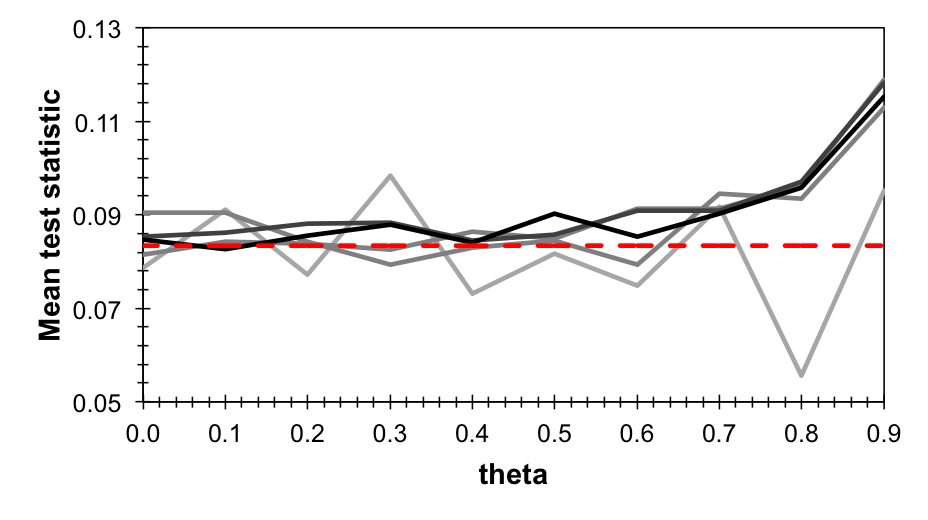
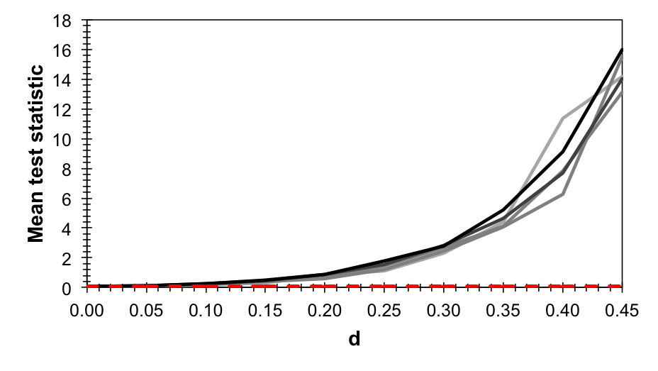
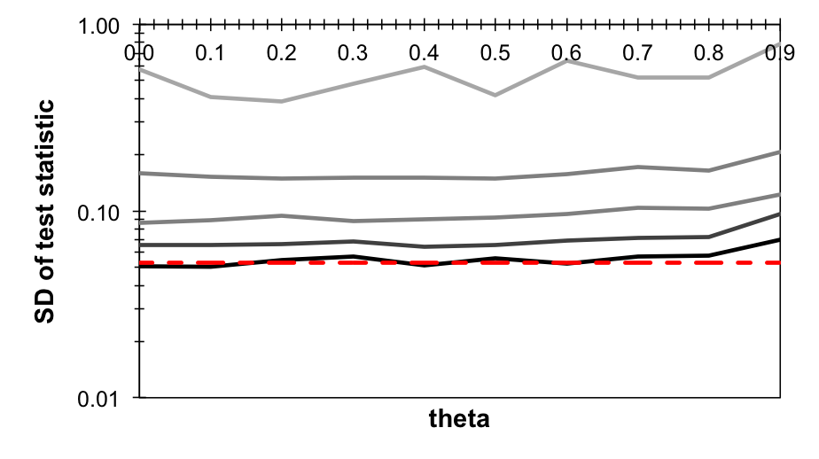
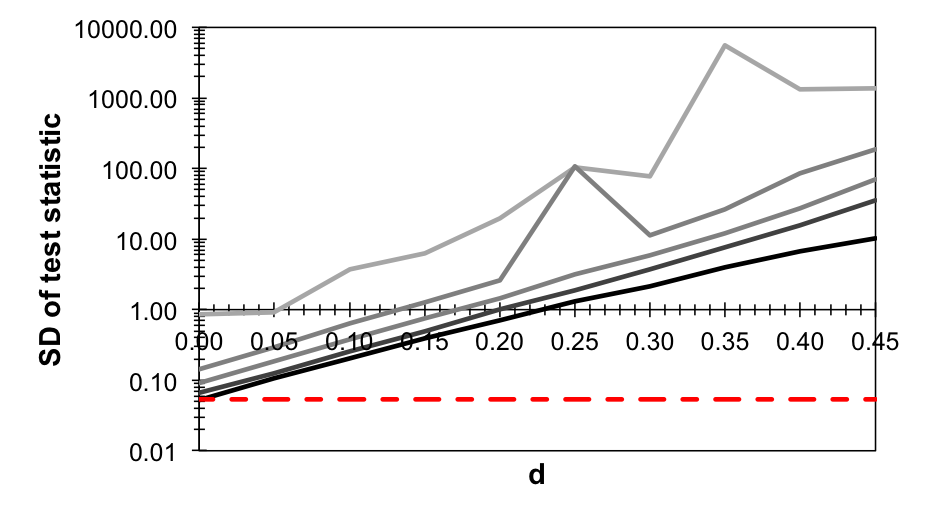
Similarly to the tests for long-range dependence in the univariate series which are based on the modified variance, such as the rescaled variance Giraitis2003 and the modified rescaled range analysis Lo1991 , the choice of parameter $q$ is crucial. If the parameter is too low, the strong short-range cross-correlations can be detected as the long-range cross-correlations and reversely, if the parameter is too high, the true long-range cross-correlations can be filtered out as the short-range ones. This issue is discussed later. Returning to the construction of RCT, the motivation was to construct a test which would have a test statistic that would be (at least partially) independent of the parameters included in the null hypothesis. For the test, we have the null hypothesis of short-range cross-correlated processes and the alternative of cross-persistent processes. Therefore, it is desirable to have a testing statistic independent of the correlation level of the short-range cross-correlated processes as well as the time decay $\delta$. In Fig. 1, we present the means and standard deviations of the testing statistics $M_{xy,T}(q)$ for both short- and long-term memory cases with varying parameters. The short-term memory processes are represented by AR(1) processes $\{x_{t}\}$ and $\{y_{t}\}$ with correlated error terms and memory parameter $\theta$:

$$x_{t}=\theta_{1}x_{t-1}+\varepsilon_{t}$$

$$y_{t}=\theta_{2}x_{t-1}+\nu_{t}$$

$$\langle\varepsilon_{t}\rangle=\langle\nu_{t}\rangle=0$$

$$\langle\varepsilon^{2}_{t}\rangle=\langle\nu^{2}_{t}\rangle=1$$

$$\langle\varepsilon_{t}\nu_{t}\rangle=\rho_{\varepsilon\nu}$$ (10)

and the long-term memory processes are covered by ARFIMA(0,$d$,0) processes $\{x_{t}\}$ and $\{y_{t}\}$ with correlated error terms:

$$x_{t}=\sum_{n=0}^{+\infty}{a_{n}(d_{1})\varepsilon_{t-n}}$$

$$y_{t}=\sum_{n=0}^{+\infty}{a_{n}(d_{2})\nu_{t-n}}$$

$$a_{n}(d_{i})=\frac{\Gamma(n+d_{i})}{\Gamma(n+1)\Gamma(d_{i})}$$

$$\langle\varepsilon_{t}\rangle=\langle\nu_{t}\rangle=0$$

$$\langle\varepsilon^{2}_{t}\rangle=\langle\nu^{2}_{t}\rangle=1$$

$$\langle\varepsilon_{t}\nu_{t}\rangle=\rho_{\varepsilon\nu}$$ (11)

To discuss the basic properties of the test, we set $\theta_{1}=\theta_{2}=\theta$ and $d_{1}=d_{2}=d$ and we fix $q=30$. Note that the fractional differencing parameter $d$ is connected to the long-term memory Hurst exponent as $H=d+0.5$. For the short-range cross-correlated processes, we observe that the mean value is remarkably stable for parameters up to $\theta=0.7$ regardless of the correlation between error terms. For higher values, the statistic deviates which can be, however, attributed to the fact that we applied $q=30$ for estimation of the test statistic and that is evidently insufficient for such a strong memory. Interestingly, the mean value of the test statistic for $0\leq\theta\leq 0.7$ practically overlays with the testing statistic of the rescaled variance test Giraitis2003 which is defined as

$$U=\int_{0}^{1}\left(W^{0}_{t}\right)^{2}dt-\left(\int_{0}^{1}W^{0}_{t}dt\right)^{2}$$ (12)

where $W^{0}_{t}$ is the standard Brownian bridge. Mean value of the statistic $U$ is equal to 1/12, which is represented by a red line in Fig. 1. In the figure, we also show behavior of the standard deviation of the statistic. Even though it is evidently dependent on the correlation between error terms of the AR(1) processes, it is remarkably stable across different levels of $\theta$. Importantly, the variance decreases with increasing correlation between error terms which is a very desirable property. For the perfectly correlated error terms of the series, the standard deviation of the statistics even attains the levels for $U$ which is equal to $1/\sqrt{360}$. For the long-range cross-correlated processes, we observe that the mean value of the statistic increases with $d$ as expected. Again, the mean value is very stable with respect to the correlation of error terms. However, the variance of the estimator increases with $d$ parameter and is also dependent on the correlations between error terms.

4 Finite sample properties

Even though the $M_{xy,T}(q)$ statistic shows some very desirable properties, we opt to base our decision in favor or against the alternative hypothesis based on the moving-block bootstrap (MBB) procedure Efron1979 ; Efron1993 ; Srinivas2000 , mainly due to dependence of the variance of the estimator on the correlations level. In the procedure, a bootstrapped series is obtained by separating the series into blocks of size $\zeta$ and shuffling the blocks, the parameter of interest is then estimated on the bootstrapped series for which the short-range dependence and the distributional properties of the original series are preserved. Based on $B$ bootstrapped estimates, the empirical confidence intervals for a specific level $\alpha$ and an empirical $p$-value are obtained. In the case of the rescaled covariance test, we work with a two-sided test with the null hypothesis of short-range cross-correlated processes against the alternative hypothesis of cross-persistence.

To examine the size and power of the test, we use the same setup as in the previous section (Eqs. 10-11). Specifically, we are interested in the finite sample properties of the rescaled covariance test for correlated, short-term correlated and long-term correlated processes with moderately and strongly correlated error terms. For the first case, we simply use a bivariate Gaussian noise series. For the second one, we utilize AR(1) processes with three levels of memory – $\theta=0.1,0.5,0.8$ – to control for weak, medium and strong cross-correlations. For the last one, we employ ARFIMA(0,$d$,0) processes with two levels of memory – $d=0.1,0.4$ – to discuss weak and strong power-law cross-correlations. For all previous cases, we discuss two levels of correlation between the error terms – 0.5 and 0.9.

For correlated but not cross-correlated processes (Table 1), we observe that the test is more precise with increasing correlation $\rho_{\varepsilon\nu}$ between error terms of the processes. For $\rho_{\varepsilon\nu}=0.9$, the size of the test practically matches the set significance levels. The size of the test gets better with increasing $q$ and practically does not vary with time series length $T$. Practically the same results are observed for the short-range cross-correlated processes as shown in Table 2. The sizes practically overlay with the theoretical values of the significance levels. These are very strong results in favor of the rescaled covariance test as it is practically intact by even very strong short-term memory. The combination of the moving-block bootstrap and HAC-estimator of covariance is evidently able to sufficiently control for possible short-term memory biases in case of the RCT test.

For long-range cross-correlated processes, we compare cases when $H_{x}=H_{y}=0.6$ and $H_{x}=H_{y}=0.9$ to distinguish between weak and strong cross-persistence. We assume these values of $H_{x}$ and $H_{y}$ in the testing procedure. The power of the test is relatively low for the weak cross-persistence case (Table 5). We, however, observe several interesting points. First, the power of the test is very similar regardless the correlation level between error terms. Second, the power of the test increases with the time series length. Third, the power increases rapidly with increasing $\alpha$. And fourthly, the power of the test even increases with an increasing $q$, which is caused by the $q^{\widehat{H_{x}}+\widehat{H_{y}}-1}$ factor in the testing statistic which well compensates for high $q$. For the strong cross-persistence (Table 6), the power of the test increases considerably and the four features of the test are the same as in the previous case. As expected, the test is more powerful with increasing $\rho_{\varepsilon\nu}$, i.e. the cross-persistence is more stable. The power of the test increases to as high as 0.967 for some cases. The test thus shows very good statistical characteristics and is well able to distinguish between short-range and long-range cross-correlations.

5 Application

In financial economics, volatility is one of the most important variables as it is utilized in option pricing, portfolio analysis and risk management. In econophysics, volatility has been frequently studied due to its power-law nature (long-term memory, extreme events and aftershocks dynamics to name the most important ones). Studying the power-law cross-correlations in financial series thus naturally leads to the financial series connected to volatility. To utilize the proposed rescaled covariance test, we analyze two pairs of series which are of the main interest in finance – volatility/returns and volatility/volume. Both pairs are interesting from the economics point of view – volatility/return relationship is known as the leverage effect as negative returns are believed to be followed by increasing volatility Cont2001 ; Bollerslev2006 , and volatility/volume pair is interesting due to the fact that both variables are influenced by similar effects and one may influence the other Karpoff1987 .

The volatility process is estimated with a use of the realized variance (volatility) approach, which employs the high-frequency data and yields consistent and efficient estimates of the true variance process Barndorff-Nielsen2002 ; Barndorff-Nielsen2002a ; Hansen2006 . The realized variance is practically the uncentered second moment of the high-frequency series during a specific day. In our case, we use the 5 minutes frequency, which provides a good balance between efficiency and market microstructure noise bias. The realized variance is then defined as

$$\widehat{\sigma^{2}_{t,RV}}=\sum_{i=1}^{n}{r^{2}_{t,i}}$$ (13)

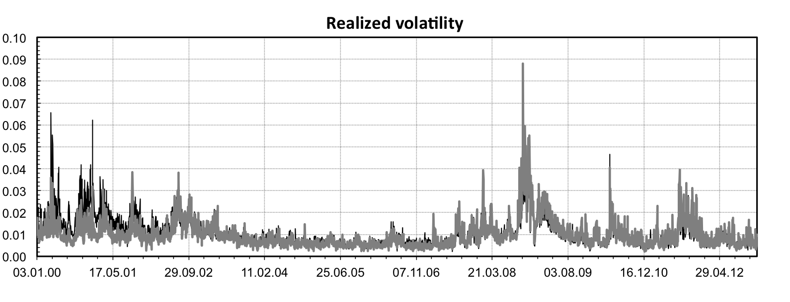
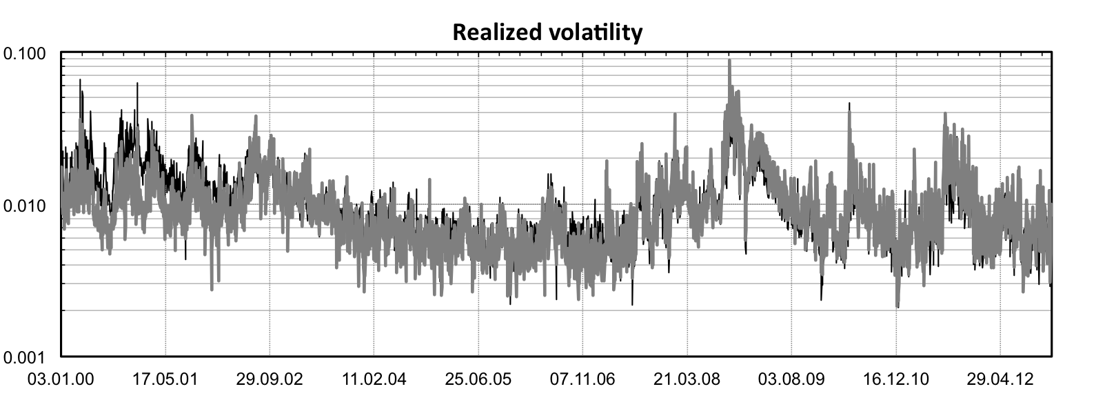
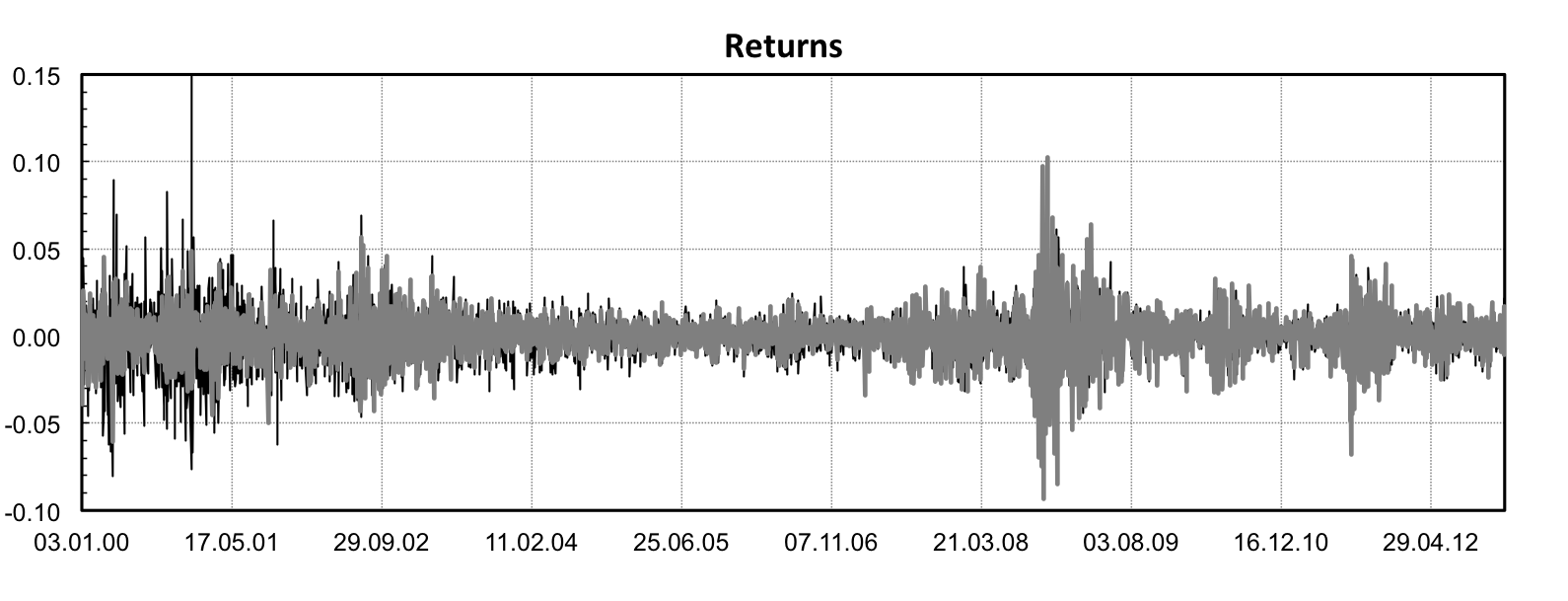
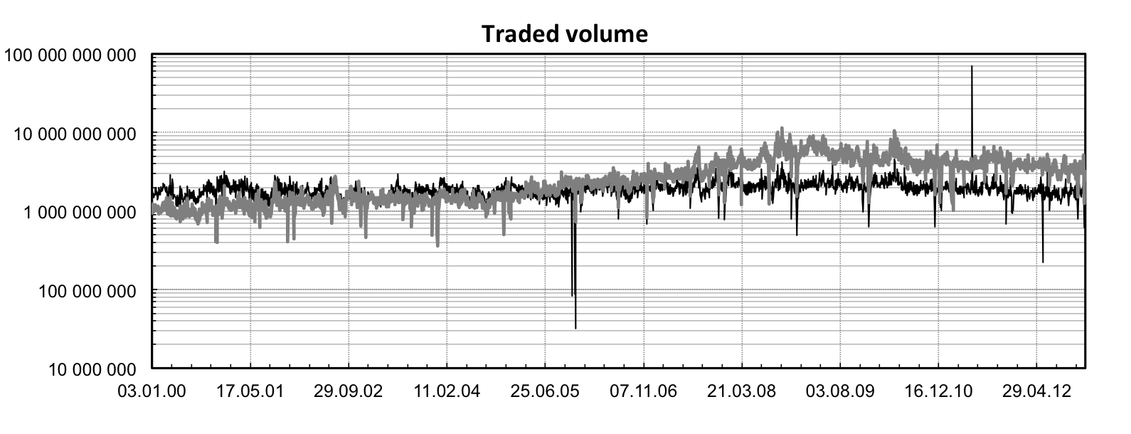
where $r_{t,i}$ is a return of the $i$-th 5-minute interval during day $t$ and $n$ is the number of these 5-minute intervals for a given day. To overcome potential problems with non-standard distribution and non-negativity of the volatility series, we focus on the logarithmic volatility, i.e. the logarithm of the square root of the realized variance, which is standardly done in the literature Muzy2000 . In our analysis, we focus on two US indices – NASDAQ-100 and S&P500 – between 1.1.2000 and 31.12.2012 (3245 and 3240 observations, respectively). In Fig. 2, we observe that returns and volatility series for both indices practically overlap and the indices experienced very similar periods of increased volatility after the DotCom bubble of 2000 and an outburst of the Global Financial Crisis in 2007/2008. Development of the traded volume differs for the indices as the volume of the NASDAQ index has been quite stable during the analyzed period while the S&P500 underwent an increasing exponential trend until the break of 2008 and 2009, stabilizing afterwards. To control for this development of the trading volume, we focus our analysis on the detrended logarithmic volume series.

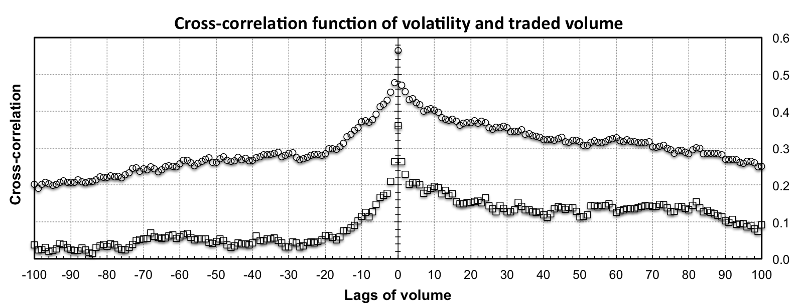
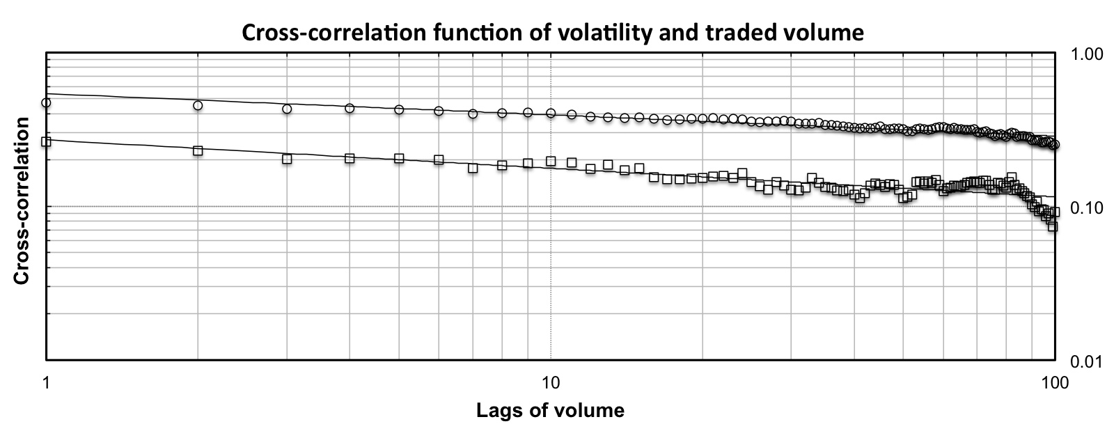
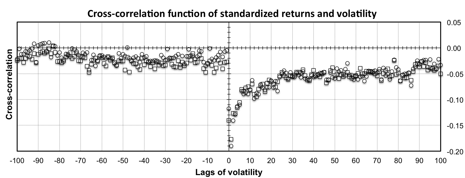
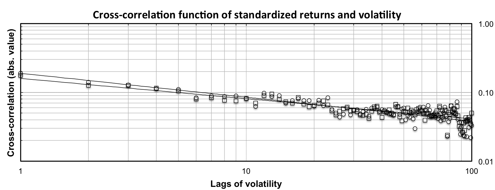
Prior to turning to the results of the rescaled covariance test, we present the cross-correlation functions for both analyzed pairs in Fig. 3. We observe that the relationships are very different from one another. Starting with the volatility/volume pair, we can see that positive cross-correlations are present for both halves of the cross-correlation function for both analyzed indices. For both, we find that the effect works in both directions. However, the effect of volatility on traded volume is more long-lasting than the other way around. Interestingly, the shape of the cross-correlation function is very similar for both indices but the level of correlations is approximately halved for NASDAQ-100 compared to the S&P500 index. Nonetheless, a simple visual detection uncovers that the pair is a good candidate for the presence of LRCC. Such statement is further supported by visible power-law scaling of the right part of the cross-correlation function shown in the right panel of Fig. 3. Turning to the returns/volatility pair, we can see a very different shape of the cross-correlation function which is strongly asymmetric. We observe a one-way effect from returns to volatility and not the other way around. Since the sample cross-correlations for the positive lags are all negative, it implies that positive (negative) returns cause, on statistical basis, decrease (increase) of volatility. This result is well in hand with the standard notion of the leverage effect in finance. Again, the decay of cross-correlations for positive lags is very slow and the pair is again a good candidate for the LRCC analysis which is visually supported by the power-law decay of the right part of the cross-correlation function illustrated in the right panel of Fig. 3. We thus have two pairs suspected to be LRCC while one being positively and the other negatively cross-persistent.

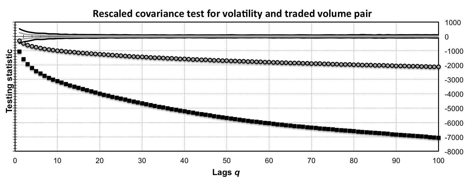
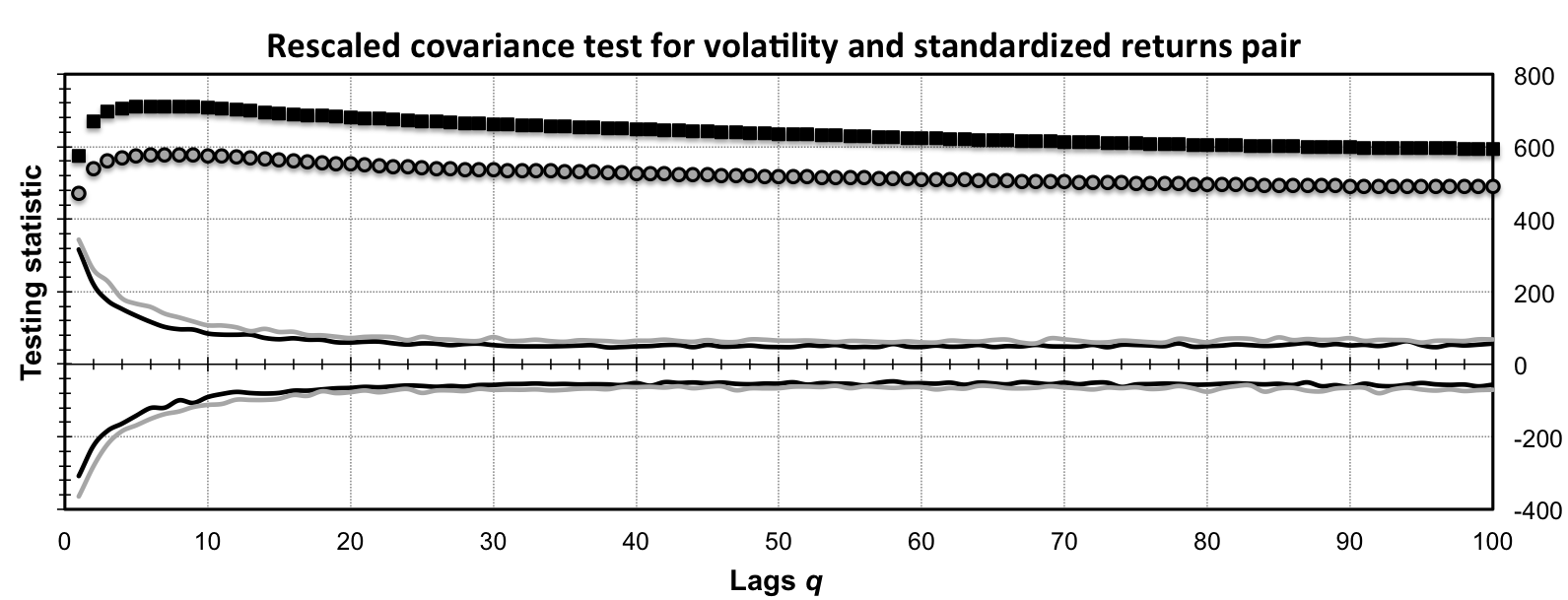
Results of the rescaled covariance test for both pairs are summarized in Fig. 4. In the figure, we present the testing statistic $M_{xy,T}(q)$ for parameter $q$ varying between 1 and 100 to see its behavior for different memory strengths. For the volatility/volume pair, we observe that the testing statistic is well below the critical values indicating statistically significant cross-persistence. This is true both for NASDAQ-100 and for S&P500. The results are robust across different lags $q$ taken into consideration and evidently, the LRCC is not spuriously found due to the short-term memory bias. For the returns/volatility pair, we again find that there is a statistical evidence of long-range cross-correlations among returns and volatility. This is again true regardless the number of lags $q$ taken into consideration. Both pairs are thus power-law cross-correlated according to the rescaled covariance test.

6 Conclusions

We introduced a new test for detection of power-law cross-correlations among a pair of time series – the rescaled covariance test. The test is based on a power-law divergence of the covariance of the partial sums of the LRCC processes. Together with a heteroskedasticity and auto-correlation robust (HAC) estimator of the long-term covariance, we developed a test with desirable statistical properties. As the application, we showed that the relationship between volatility and traded volume, and volatility and returns in the financial markets can be labeled as the one with power-law cross-correlations. Such test should be used as a starting point in the analysis of long-range cross-correlations prior to an estimation of bivariate long-term memory parameters.

Figure 1: Mean values and standard deviations of RCT test. Test statistic $M_{xy,5000}(30)$ for differently correlated processes. Correlation between error terms varies between 0.2 and 1 with a step of 0.2 and the darker the line in the chart is, the higher the correlation is. On the left, correlated AR(1) processes with $\theta$ ranging between 0 and 0.9 with a step of 0.1 are shown. On the right, correlated ARFIMA(0,$d$,0) processes with $d$ ranging between 0 and 0.45 with a step of 0.05 are shown. Means are based on 1,000 simulations with a time series length of 5,000 and presented in a semi-log scale for better legibility.

Figure 2: Volatility, returns and traded volume of NASDAQ-100 and S&P500. Realized volatility (top left), logarithmic realized volatility (top right), logarithmic returns (bottom left) and logarithmic traded volume (bottom right) are shown for NASDAQ-100 (in black) and S&P500 (in grey).

Figure 3: Cross-correlation functions for returns, volatility and traded volume of NASDAQ-100 and S&P500. Cross-correlatios among volatility and traded volume (top left and in log-log scale in top right), and among returns and volatility (bottom left and in log-log scale in bottom right) are shown for NASDAQ-100 ($\square$) and S&P500 ($\circ$).

Figure 4: Rescaled covariance statistics $M_{xy,T}(q)$ for NASDAQ-100 and S&P500. Testing statistics are shown for varying $q$ parameter between 1 and 100 to control for short-term memory. The statistics are shown for NASDAQ-100 ($\square$) and S&P500 ($\circ$) and the 95% confidence intervals are shown in solid lines (black for NASDAQ-100 and grey for S&P500). If the testing statistics lay outside of the confidence intervals, the null hypothesis of no LRCC is rejected. The results are shown for the volatility-volume (left) and returns-volatility (right) pairs.

Table 1: Size of $M_{xy,T}(q)$ statistic I. Monte-Carlo-based test size for 1,000 replications of processes $x_{t}=\varepsilon_{t}$ and $y_{t}=\nu_{t}$ with different correlations $\rho_{\varepsilon\nu}$.

			$\rho=0.5$			$\rho=0.9$
		$\alpha=0.01$	$\alpha=0.05$	$\alpha=0.1$	$\alpha=0.01$	$\alpha=0.05$	$\alpha=0.1$
	$q=1$	0.011	0.045	0.092	0.011	0.050	0.099
$T=500$	$q=5$	0.009	0.042	0.092	0.010	0.050	0.099
	$q=10$	0.011	0.042	0.090	0.011	0.052	0.102
	$q=30$	0.011	0.042	0.090	0.011	0.052	0.102
	$q=1$	0.011	0.048	0.101	0.014	0.062	0.094
$T=1000$	$q=5$	0.012	0.052	0.101	0.014	0.060	0.094
	$q=10$	0.011	0.053	0.100	0.014	0.053	0.095
	$q=30$	0.011	0.053	0.100	0.014	0.053	0.095
	$q=1$	0.014	0.047	0.100	0.012	0.049	0.101
$T=5000$	$q=5$	0.014	0.048	0.102	0.012	0.050	0.100
	$q=10$	0.014	0.048	0.098	0.012	0.050	0.099
	$q=30$	0.014	0.048	0.098	0.012	0.050	0.099

Table 2: Size of $M_{xy,T}(q)$ statistic II. Monte-Carlo-based test size for 1,000 replications of two AR(1) processes with $\theta_{x}=\theta_{y}=0.1$ and different correlations $\rho_{\varepsilon\nu}$.

			$\rho=0.5$			$\rho=0.9$
		$\alpha=0.01$	$\alpha=0.05$	$\alpha=0.1$	$\alpha=0.01$	$\alpha=0.05$	$\alpha=0.1$
	$q=1$	0.006	0.045	0.109	0.009	0.036	0.084
$T=500$	$q=5$	0.005	0.048	0.104	0.009	0.038	0.082
	$q=10$	0.006	0.048	0.108	0.007	0.034	0.085
	$q=30$	0.006	0.048	0.108	0.007	0.034	0.085
	$q=1$	0.013	0.061	0.102	0.018	0.049	0.093
$T=1000$	$q=5$	0.010	0.063	0.104	0.017	0.049	0.087
	$q=10$	0.010	0.058	0.105	0.018	0.048	0.090
	$q=30$	0.010	0.058	0.105	0.018	0.048	0.090
	$q=1$	0.014	0.054	0.117	0.011	0.050	0.109
$T=5000$	$q=5$	0.014	0.053	0.114	0.012	0.050	0.110
	$q=10$	0.014	0.051	0.115	0.012	0.052	0.109
	$q=30$	0.014	0.051	0.115	0.012	0.052	0.109

Table 3: Size of $M_{xy,T}(q)$ statistic III. Monte-Carlo-based test size for 1,000 replications of two AR(1) processes with $\theta_{x}=\theta_{y}=0.5$ and different correlations $\rho_{\varepsilon\nu}$.

			$\rho=0.5$			$\rho=0.9$
		$\alpha=0.01$	$\alpha=0.05$	$\alpha=0.1$	$\alpha=0.01$	$\alpha=0.05$	$\alpha=0.1$
	$q=1$	0.006	0.044	0.101	0.012	0.046	0.095
$T=500$	$q=5$	0.003	0.043	0.095	0.012	0.047	0.084
	$q=10$	0.005	0.044	0.092	0.009	0.046	0.083
	$q=30$	0.005	0.044	0.092	0.009	0.046	0.083
	$q=1$	0.011	0.057	0.103	0.012	0.049	0.104
$T=1000$	$q=5$	0.009	0.053	0.099	0.012	0.046	0.096
	$q=10$	0.008	0.052	0.093	0.012	0.043	0.096
	$q=30$	0.008	0.052	0.093	0.012	0.043	0.096
	$q=1$	0.006	0.047	0.090	0.015	0.053	0.106
$T=5000$	$q=5$	0.006	0.042	0.083	0.013	0.055	0.107
	$q=10$	0.005	0.043	0.079	0.012	0.056	0.106
	$q=30$	0.005	0.043	0.079	0.012	0.056	0.106

Table 4: Size of $M_{xy,T}(q)$ statistic IV. Monte-Carlo-based test size for 1,000 replications of two AR(1) processes with $\theta_{x}=\theta_{y}=0.8$ and different correlations $\rho_{\varepsilon\nu}$.

			$\rho=0.5$			$\rho=0.9$
		$\alpha=0.01$	$\alpha=0.05$	$\alpha=0.1$	$\alpha=0.01$	$\alpha=0.05$	$\alpha=0.1$
	$q=1$	0.019	0.075	0.135	0.010	0.048	0.104
$T=500$	$q=5$	0.013	0.063	0.120	0.008	0.048	0.100
	$q=10$	0.011	0.058	0.116	0.009	0.047	0.094
	$q=30$	0.011	0.058	0.116	0.009	0.047	0.094
	$q=1$	0.020	0.068	0.130	0.014	0.050	0.097
$T=1000$	$q=5$	0.015	0.059	0.121	0.012	0.045	0.085
	$q=10$	0.012	0.054	0.110	0.011	0.047	0.083
	$q=30$	0.012	0.054	0.110	0.011	0.047	0.083
	$q=1$	0.017	0.072	0.120	0.022	0.065	0.108
$T=5000$	$q=5$	0.016	0.064	0.111	0.017	0.054	0.104
	$q=10$	0.013	0.058	0.104	0.017	0.053	0.102
	$q=30$	0.013	0.058	0.104	0.017	0.053	0.102

Table 5: Power of $M_{xy,T}(q)$ statistic I. Monte-Carlo-based test power for 1,000 replications of two ARFIMA(0,$d$,0) processes with $d_{x}=d_{y}=0.1$ and different correlations $\rho_{\varepsilon\nu}$.

			$\rho=0.5$			$\rho=0.9$
		$\alpha=0.01$	$\alpha=0.05$	$\alpha=0.1$	$\alpha=0.01$	$\alpha=0.05$	$\alpha=0.1$
	$q=1$	0.018	0.087	0.148	0.029	0.094	0.141
$T=500$	$q=5$	0.081	0.184	0.275	0.103	0.196	0.278
	$q=10$	0.117	0.232	0.343	0.142	0.254	0.344
	$q=30$	0.117	0.232	0.343	0.142	0.254	0.344
	$q=1$	0.030	0.111	0.172	0.023	0.090	0.166
$T=1000$	$q=5$	0.097	0.205	0.295	0.094	0.215	0.312
	$q=10$	0.135	0.252	0.349	0.155	0.283	0.369
	$q=30$	0.135	0.252	0.349	0.155	0.283	0.369
	$q=1$	0.091	0.200	0.283	0.090	0.201	0.282
$T=5000$	$q=5$	0.187	0.320	0.409	0.195	0.342	0.438
	$q=10$	0.233	0.368	0.466	0.235	0.399	0.500
	$q=30$	0.233	0.368	0.466	0.235	0.399	0.500

Table 6: Power of $M_{xy,T}(q)$ statistic II. Monte-Carlo-based test power for 1,000 replications of two ARFIMA(0,$d$,0) processes with $d_{x}=d_{y}=0.4$ and different correlations $\rho_{\varepsilon\nu}$.

			$\rho=0.5$			$\rho=0.9$
		$\alpha=0.01$	$\alpha=0.05$	$\alpha=0.1$	$\alpha=0.01$	$\alpha=0.05$	$\alpha=0.1$
	$q=1$	0.111	0.229	0.318	0.147	0.272	0.356
$T=500$	$q=5$	0.649	0.725	0.768	0.734	0.797	0.839
	$q=10$	0.772	0.830	0.862	0.869	0.904	0.924
	$q=30$	0.772	0.830	0.862	0.869	0.904	0.924
	$q=1$	0.205	0.339	0.421	0.255	0.371	0.464
$T=1000$	$q=5$	0.697	0.774	0.814	0.747	0.813	0.846
	$q=10$	0.817	0.867	0.891	0.857	0.893	0.914
	$q=30$	0.817	0.867	0.891	0.857	0.893	0.914
	$q=1$	0.464	0.584	0.636	0.584	0.685	0.737
$T=5000$	$q=5$	0.823	0.878	0.899	0.892	0.922	0.934
	$q=10$	0.898	0.922	0.933	0.934	0.958	0.967
	$q=30$	0.898	0.922	0.933	0.934	0.958	0.967

Appendix

Proof to “Partial sum covariance scaling” proposition

Using the zero mean and stationarity properties of processes $\{x_{t}\}$ and $\{y_{t}\}$, we can write the covariance of the partial sums as

$$\text{Cov}(X_{n},Y_{n})=\langle X_{n}Y_{n}\rangle=\sigma_{x}\sigma_{y}\Big{(}n\rho_{xy}(0)+\sum_{k=1}^{n-1}(n-k)(\rho_{xy}(k)+\rho_{xy}(-k))\Big{)}\\ \propto n\rho_{xy}(0)+\sum_{k=1}^{n-1}(n-k)(\rho_{xy}(k)+\rho_{xy}(-k)).$$ (14)

Now, assuming that $\rho_{xy}(k)$ is symmetric for $k>0$ and $k<0$, we have

$$\text{Cov}(X_{n},Y_{n})\propto n\rho_{xy}(0)+n\sum_{k=1}^{n-1}{\rho_{xy}(k)}-\sum_{k=1}^{n-1}{k\rho_{xy}(k)}.$$ (15)

Using the LRCC definition and approximating the infinite sums with definite integrals according to the Euler–MacLaurin integration formula [14, 38], we get

$$n\sum_{k=1}^{n-1}{\rho_{xy}(k)}\propto n\sum_{k=1}^{n-1}k^{-\gamma_{xy}}\approx n\int_{1}^{n}{k^{-\gamma_{xy}}dk}\propto n^{2-\gamma_{xy}},$$ (16)

$$\sum_{k=1}^{n-1}{k\rho_{xy}(k)}\propto\sum_{k=1}^{n-1}k^{1-\gamma_{xy}}\approx\int_{1}^{n}{k^{1-\gamma_{xy}}dk}\propto n^{2-\gamma_{xy}}.$$ (17)

Finally, we use that the linear growth of $n\rho_{xy}(0)$ is asymptotically dominated by the power-law growth in the latter terms, i.e. using the l’Hôpital’s rule we have

$$\lim_{n\rightarrow+\infty}{\frac{n^{2-\gamma_{xy}}}{n\rho_{xy}(0)}}=\lim_{n\rightarrow+\infty}{\frac{(2-\gamma_{xy})n^{1-\gamma_{xy}}}{\rho_{xy}(0)}}=+\infty\text{ for }0<\gamma_{xy}<1$$ (18)

and we get

$$\text{Cov}(X_{n},Y_{n})\propto n^{2-\gamma_{xy}}\text{ as }n\rightarrow+\infty.$$ (19)

Note that the substitutions in Eqs. 16 and 17 from $\sum_{k=1}^{n-1}{\rho_{xy}(k)}$ to $\sum_{k=1}^{n-1}{k^{-\gamma_{xy}}}$ are done for $k$ between $1$ and $n-1$ without a loss on generality as we are interested in the asymptotic properties of Cov($X_{n},Y_{n}$).

Further, we have $2H_{xy}=2-\gamma_{xy}$ so that

$$H_{xy}=1-\frac{\gamma_{xy}}{2}.$$ (20)

For the asymmetric cross-correlation function, the results do not differ significantly. We have

$$\text{Cov}(X_{n},Y_{n})\approx n\rho_{xy}(0)+\underbrace{n\sum_{k=1}^{n-1}{k^{-\gamma^{1}_{xy}}}-\sum_{k=1}^{n-1}{k^{-\gamma^{1}_{xy}+1}}}_{\propto n^{2-\gamma^{1}_{xy}}}+\underbrace{n\sum_{k=1}^{n-1}{k^{-\gamma^{2}_{xy}}}-\sum_{k=1}^{n-1}{k^{-\gamma^{2}_{xy}+1}}}_{\propto n^{2-\gamma^{2}_{xy}}},$$ (21)

where the approximate proportionality comes from Eqs. 16 and 17. Asymptotically, the power-law scaling is dominated by the higher exponent, i.e. the lower $\gamma_{xy}$. For $\gamma_{xy}^{1}<\gamma_{xy}^{2}$, we have $\text{Cov}(X_{n},Y_{n})\sim n^{2-\gamma_{xy}^{1}}$ and vice versa. Note that the lower $\gamma_{xy}$ is connected to the higher bivariate Hurst exponent $H_{xy}$ which implies that the scaling of covariances is dominated by the stronger cross-persistence. $\square$

Proof to “Diverging limit of covariance of partial sums” proposition

We have

$$\lim_{n\rightarrow+\infty}{\frac{\text{Cov}(X_{n},Y_{n})}{n}}\propto\lim_{n\rightarrow+\infty}\frac{n^{2H_{xy}}}{n}=\lim_{n\rightarrow+\infty}\frac{n^{2-\gamma_{xy}}}{n}=\\ \lim_{n\rightarrow+\infty}n^{1-\gamma_{xy}}=+\infty\text{ for }0<\gamma_{xy}<1.\square$$ (22)

Proof to “Converging limit of covariance of partial sums” proposition

In accordance with the proof for the LRCC case, we assume a symmetric cross-correlation function so that we can write

$$\text{Cov}(X_{n},Y_{n})\propto n\rho_{xy}(0)+n\sum_{k=1}^{n-1}{\rho_{xy}(k)}-\sum_{k=1}^{n-1}{k\rho_{xy}(k)}.$$ (23)

It holds that

$$\lim_{n\rightarrow+\infty}{\frac{\text{Cov}(X_{n},Y_{n})}{n}}\propto\lim_{n\rightarrow+\infty}{\left(\rho_{xy}(0)+\sum_{k=1}^{n-1}{\rho_{xy}(k)}-\frac{1}{n}\sum_{k=1}^{n-1}{k\rho_{xy}(k)}\right)}.$$ (24)

Solving the sums separately with a use of short-range cross-correlations definition, we get

$$\sum_{k=1}^{n-1}{\rho_{xy}(k)}\propto\sum_{k=1}^{n-1}{\exp\left(-\frac{k}{\delta}\right)}\propto\frac{1-\exp\left(-\frac{n}{\delta}\right)}{1-\exp\left(-\frac{1}{\delta}\right)}$$ (25)

$$\sum_{k=1}^{n-1}{k\rho_{xy}(k)}\propto\sum_{k=1}^{n-1}{k\exp\left(-\frac{k}{\delta}\right)}=\exp\left(-\frac{1}{\delta}\right)-n\exp\left(-\frac{n}{\delta}\right)+(n-1)\exp\left(-\frac{n+1}{\delta}\right)$$ (26)

Substituting back, we obtain

$$\lim_{n\rightarrow+\infty}{\frac{\text{Cov}(X_{n},Y_{n})}{n}}\propto\lim_{n\rightarrow+\infty}\Bigg{[}\rho_{xy}(0)+\frac{1-\exp\left(-\frac{n}{\delta}\right)}{1-\exp\left(-\frac{1}{\delta}\right)}-\frac{\exp\left(-\frac{1}{\delta}\right)}{n}+\\ \frac{n}{n}\exp\left(-\frac{n}{\delta}\right)+\frac{n-1}{n}\exp\left(-\frac{n+1}{\delta}\right)\Bigg{]}=\rho_{xy}(0)+\frac{1}{1-\exp\left(-\frac{1}{\delta}\right)}$$ (27)

and the limit evidently converges for $0\leq\delta<+\infty$ which concludes the proof. $\square$

References

- [1] J. Alvarez-Ramirez and R. Escarela-Perez. Time-dependent correlations in electricity markets. Energy Economics, 32(2):269–277, 2010.
- [2] O. Barndorff-Nielsen and N. Shephard. Econometric analysis of realised volatility and its ise in estimating stochastic volatility models. Journal of the Royal Statistical Society: Series B, 64:253–280, 2002.
- [3] O. Barndorff-Nielsen and N. Shephard. Estimating quadratic variation using realized variance. Journal of Applied Econometrics, 17(5):457–477, 2002.
- [4] J. Barunik, T. Aste, T. Di Matteo, and R. Liu. Understanding the source of multifractality in financial markets. Physica A, 391:4234–4251, 2012.
- [5] J. Barunik and L. Kristoufek. On Hurst exponent estimation under heavy-tailed distributions. Physica A, 389(18):3844–3855, 2010.
- [6] J. Beran. Statistics for Long-Memory Processes, volume 61 of Monographs on Statistics and Applied Probability. Chapman and Hall, New York, 1994.
- [7] T. Bollerslev, J. Litvinova, and G. Tauchen. Leverage and volatility feedback effects in high-frequency data. Journal of Financial Econometrics, 4(3):353–384, 2006.
- [8] A. Chakraborti, I.M. Toke, M. Patriarca, and F. Abergel. Econophysics review: I. Empirical facts. Quantitative Finance, 11(7):991–1012, 2011.
- [9] R. Cont. Empirical properties of asset returns: stylized facts and statistical issues. Quantitative Finance, 1(2)(2):223 – 236, 2001.
- [10] M. Couillard and M. Davison. A comment on measuring the hurst exponent of financial time series. Physica A, 348:404–418, 2005.
- [11] T. Di Matteo. Multi-scaling in finance. Quantitatice Finance, 7(1):21–36, 2007.
- [12] B. Efron. Bootstrap methods: Another look at the jacknife. Annals of Statistics, 7(1):1–26, 1979.
- [13] B. Efron, R. Tibshirani, and R.J. Tibshirani. An introduction to the bootstrap. Chapman & Hall, 1993.
- [14] L. Euler. Methodus generalis summandi progressiones. Commentarii Academiae Scientiarum Petropolitanae, 6:68–97, 1738.
- [15] J. Fleming and C. Kirby. Long memory in volatility and trading volume. Journal of Banking & Finance, 35:1714–1726, 2011.
- [16] L. Giraitis, P. Kokoszka, R. Leipus, and G. Teyssière. Rescaled variance and related tests for long memory in volatility and levels. Journal of Econometrics, 112:265–294, 2003.
- [17] P. Gopikrishnan, V. Plerou, Y. Liu, L.A.N. Amaral, X. Gabaix, and H.E. Stanley. Scaling and correlation in financial time series. Physica A, 287:362–373, 2000.
- [18] D. Grech and Z. Mazur. Statistical properties of old and new techniques in detrended analysis of time series. Acta Physica Polonica B, 36:2403–2413, 2005.
- [19] G.-F. Gu and W.-X. Zhou. Detrending moving average algorithm for multifractals. Physical Review E, 82:011136, 2010.
- [20] P. Hansen and A. Lunde. Realized variance and market microstructure noise. Journal of Business and Economic Statistics, 24:127–218, 2006.
- [21] L.-Y. He and S.-P. Chen. Multifractal detrended cross-correlation analysis of agricultural futures markets. Chaos, Solitons and Fractals, 44:355–361, 2011.
- [22] L.-Y. He and S.-P. Chen. A new approach to quantify power-law cross-correlation and its application to commodity markets. Physica A, 390:3806–3814, 2011.
- [23] L.-Y. He and S.-P. Chen. Nonlinear bivariate dependency of price volume relationships in agricultural commodity futures markets: A perspective from Multifractal Detrended Cross-Correlation Analysis. Physica A, 390:297–308, 2011.
- [24] H.E. Hurst. Long term storage capacity of reservoirs. Transactions of the American Society of Engineers, 116:770–799, 1951.
- [25] Z.-Q. Jiang and W.-X. Zhou. Multifractal detrending moving average cross-correlation analysis. Physical Review E, 84:016106, 2011.
- [26] J. Kantelhardt, S. Zschiegner, E. Koscielny-Bunde, A. Bunde, S. Havlin, and H. E. Stanley. Multifractal Detrended Fluctuation Analysis of Nonstationary Time Series. Physica A, 316(1-4):87–114, 2002.
- [27] J.M. Karpoff. The Relationship between Price Changes and Trading Volume: A Survey. Journal of Financial and Quantitative Analysis, 22(1):109–126, 1987.
- [28] L. Kristoufek. Long-range dependence in returns and volatility of Central European stock indices. Bulletin of the Czech Econometric Society, 17(27):50–67, 2010.
- [29] L. Kristoufek. On spurious anti-persistence in the US stock indices. Chaos, Solitons and Fractals, 43:68–78, 2010.
- [30] L. Kristoufek. Rescaled range analysis and detrended fluctuation analysis: Finite sample properties and confidence intervals. AUCO Czech Economic Review, 4:236–250, 2010.
- [31] L. Kristoufek. Multifractal height cross-correlation analysis: A new method for analyzing long-range cross-correlations. EPL, 95:68001, 2011.
- [32] L. Kristoufek. How are rescaled range analyses affected by different memory and distributional properties? A Monte Carlo study. Physica A, 391:4252–4260, 2012.
- [33] D. Kwiatkowski, P. Phillips, P. Schmidt, and Y. Shin. Testing the null of stationarity against alternative of a unit root: How sure are we that the economic time series have a unit root? Journal of Econometrics, 54:159–178, 1992.
- [34] F. Lavancier, A. Philippe, and D. Surgailis. Atwo-sampletest for comparison of longmemoryparameters. Journal of Multivariate Analysis, 101(9):2118–2136, 2010.
- [35] Y. Liu, P. Gopikrishnan, P. Cizeau, M. Meyer, C.-K. Peng, and H.E. Stanley. Statistical properties of the volatility price fluctuations. Physical Review E, 60(2):1390–1400, 1999.
- [36] A. Lo. Long-term memory in stock market prices. Econometrica, 59(5):1279–1313, 1991.
- [37] F. Ma, Y. Wei, and D. Huang. Multifractal detrended cross-correlation analysis between the Chinese stock market and surrounding stock markets. Physica A, 392:1659–1670, 2013.
- [38] C. MacLaurin. A Treatuse of Fluxions. T.W. and T. Ruddimans, 1742.
- [39] B. Mandelbrot and J. Wallis. Joah, joseph and operational hydrology. Water Resources Research, 4(5):909–918, 1968.
- [40] R.N. Mantegna and H.E. Stanley. An Introduction to EconophysicsL Correlations and Complexity in Finance. Cambridge University Press, 1999.
- [41] J.-F. Muzy, J. Delour, and E. Bacry. Modeling fluctuations of financial time series: from cascade processes to stochastic volatility models. European Physical Journal B, 17(3):537–548, 2000.
- [42] C. Peng, S. Buldyrev, A. Goldberger, S. Havlin, M. Simons, and H. E. Stanley. Finite-size effects on long-range correlations: Implications for analyzing DNA sequences. Physical Review E, 47(5):3730–3733, 1993.
- [43] C. Peng, S. Buldyrev, S. Havlin, M. Simons, H. E. Stanley, and A. Goldberger. Mosaic organization of DNA nucleotides. Physical Review E, 49(2):1685–1689, 1994.
- [44] V. Plerou, P. Gopikrishnan, B. Rosenow, L.A.N. Amaral, and H.E. Stanley. Econophysics: financial time series from a statistical physics point of view. Physica A, 279:443–456, 2000.
- [45] B. Podobnik, I. Grosse, D. Horvatic, S. Ilic, P. Ch. Ivanov, and H. E. Stanley. Quantifying cross-correlations using local and global detrending approaches. European Physical Journal B, 71:243–250, 2009.
- [46] B. Podobnik, D. Horvatic, A. Petersen, and H. E. Stanley. Cross-correlations between volume change and price change. Proceedings of the National Academy of Sciences of the United States of America, 106(52):22079–22084, 2009.
- [47] B. Podobnik, Z.-Q. Jiang, W.-X. Zhou, and H. E. Stanley. Statistical tests for power-law cross-correlated processes. Physical Review E, 84:066118, 2011.
- [48] B. Podobnik and H.E. Stanley. Detrended cross-correlation analysis: A new method for analyzing two nonstationary time series. Physical Review Letters, 100:084102, 2008.
- [49] G. Power and C. Turvey. Long-range dependence in the volatility of commodity futures prices: Wavelet-based evidence. Physica A, 389:79–90, 2010.
- [50] Gennady Samorodnitsky. Long range dependence. Foundation and Trends® in Stochastic Systems, 1(3):163–257, 2006.
- [51] R. Sela and C. Hurvich. The average periodogram estimator for a power law in coherency. Journal of Time Series Analysis, 33:340–363, 2012.
- [52] E. L. Siqueira Jr., T. Stošić, L. Bejan, and B. Stošić. Correlations and cross-correlations in the Brazilian agrarian commodities and stocks. Physica A, 389:2739–2743, 2010.
- [53] V. Srinivas and K. Srinivasan. Post-blackening approach for modeling dependent annual streamflows. Journal of Hydrology, 230:86–126, 2000.
- [54] M. Taqqu, W. Teverosky, and W. Willinger. Estimators for long-range dependence: an empirical study. Fractals, 3(4):785–798, 1995.
- [55] M. Taqqu and V. Teverovsky. On Estimating the Intensity of Long-Range Dependence in Finite and Infinite Variance Time Series. In A Practical Guide To Heavy Tails: Statistical Techniques and Applications, 1996.
- [56] M. Taqqu and V. Teverovsky. A practical guide to heavy tails: statistical techniques and applications, chapter On estimating the intensity of long-range dependence in finite and infinite variance time series, pages 177–217. Birkhauser Boston Inc., 1998.
- [57] D.-H. Wang, Y.-Y. Suo, X.-W. Yu, and M. Lei. Price-volume cross-correlation analysis pf CSI300 index futures. Physica A, 392:1172–1179, 2013.
- [58] G.-J. Wang and C. Xie. Cross-correlations between Renminbi and four major currencies in the Renminbi currency basket. Physica A, 392:1418–1428, 2013.
- [59] J. Wang, P. Shang, and W. Ge. Multifractal cross-correlation analysis based on statistical moments. Fractals, 20(3):271–279, 2012.
- [60] R. Weron. Estimating long-range dependence: Finite sample properties and confidence intervals. Physica A, 312:285–299, 2002.
- [61] G.F. Zebende. DCCA cross-correlation coefficient: Quantifying level of cross-correlation. Physica A, 390:614–618, 2011.
- [62] W.-X. Zhou. Multifractal detrended cross-correlation analysis for two nonstationary signals. Physical Review E, 77:066211, 2008.