1 Introduction
As in [5 ] ,
we consider the standard elliptic Dirichlet boundary value problem
− div A ∇ u div 𝐴 ∇ 𝑢 \displaystyle-\operatorname{div}A\nabla u = f absent 𝑓 \displaystyle=f in Ω , in Ω \displaystyle\text{in }\Omega, (1.1)
u 𝑢 \displaystyle u = u 0 absent subscript 𝑢 0 \displaystyle=u_{0} on Γ , on Γ \displaystyle\text{on }\Gamma, (1.2)
where Ω ⊂ ℝ N Ω superscript ℝ 𝑁 \Omega\subset\mathbb{R}^{N} N ≥ 3 𝑁 3 N\geq 3 Γ := ∂ Ω assign Γ Ω \Gamma:=\operatorname{\partial}\!\Omega A : Ω → ℝ N × N : 𝐴 → Ω superscript ℝ 𝑁 𝑁 A:\Omega\to\mathbb{R}^{N\times N} 𝖫 ∞ ( Ω ) superscript 𝖫 Ω \operatorname{\mathsf{L}}^{\infty}(\Omega)
∃ α > 0 ∀ ξ ∈ ℝ N ∀ x ∈ Ω A ( x ) ξ ⋅ ξ ≥ α − 2 | ξ | 2 formulae-sequence 𝛼 0 formulae-sequence for-all 𝜉 superscript ℝ 𝑁 formulae-sequence for-all 𝑥 Ω ⋅ 𝐴 𝑥 𝜉 𝜉 superscript 𝛼 2 superscript 𝜉 2 \exists\,\alpha>0\quad\forall\,\xi\in\mathbb{R}^{N}\quad\forall\,x\in\Omega\qquad A(x)\xi\cdot\xi\geq\alpha^{-2}|\xi|^{2}
holds. As usual, when working with exterior domain problems,
we use the polynomially weighted Lebesgue spaces
𝖫 s 2 ( Ω ) := { u : ρ s u ∈ 𝖫 2 ( Ω ) } , ρ := ( 1 + r 2 ) 1 / 2 ≅ r , s ∈ ℝ , formulae-sequence formulae-sequence assign subscript superscript 𝖫 2 𝑠 Ω conditional-set 𝑢 superscript 𝜌 𝑠 𝑢 superscript 𝖫 2 Ω assign 𝜌 superscript 1 superscript 𝑟 2 1 2 𝑟 𝑠 ℝ \operatorname{\mathsf{L}}^{2}_{s}(\Omega):=\{u\,:\,\rho^{s}u\in\operatorname{\mathsf{L}}^{2}(\Omega)\},\quad\rho:=(1+r^{2})^{1/2}\cong r,\quad s\in\mathbb{R},
where r ( x ) := | x | assign 𝑟 𝑥 𝑥 r(x):=|x| s ∈ { − 1 , 0 , 1 } 𝑠 1 0 1 s\in\{-1,0,1\} s = 0 𝑠 0 s=0 𝖫 2 ( Ω ) := 𝖫 0 2 ( Ω ) assign superscript 𝖫 2 Ω subscript superscript 𝖫 2 0 Ω \operatorname{\mathsf{L}}^{2}(\Omega):=\operatorname{\mathsf{L}}^{2}_{0}(\Omega)
𝖧 ( Ω ) − 1 1 \displaystyle\overset{}{\operatorname{\mathsf{H}}}{}^{1}_{-1}(\Omega) := { u : u ∈ 𝖫 − 1 2 ( Ω ) , ∇ u ∈ 𝖫 2 ( Ω ) } , assign absent conditional-set 𝑢 formulae-sequence 𝑢 subscript superscript 𝖫 2 1 Ω ∇ 𝑢 superscript 𝖫 2 Ω \displaystyle:=\{u\,:\,u\in\operatorname{\mathsf{L}}^{2}_{-1}(\Omega),\,\nabla u\in\operatorname{\mathsf{L}}^{2}(\Omega)\},
𝖣 ( Ω ) absent 𝖣 Ω \displaystyle\overset{}{\operatorname{\mathsf{D}}}(\Omega) := { v : v ∈ 𝖫 2 ( Ω ) , div v ∈ 𝖫 1 2 ( Ω ) } , assign absent conditional-set 𝑣 formulae-sequence 𝑣 superscript 𝖫 2 Ω div 𝑣 subscript superscript 𝖫 2 1 Ω \displaystyle:=\{v\,:\,v\in\operatorname{\mathsf{L}}^{2}(\Omega),\,\operatorname{div}v\in\operatorname{\mathsf{L}}^{2}_{1}(\Omega)\},
which we equip as 𝖫 s 2 ( Ω ) subscript superscript 𝖫 2 𝑠 Ω \operatorname{\mathsf{L}}^{2}_{s}(\Omega)
𝖧 ∘ ( Ω ) − 1 1 := 𝖢 ∘ ( Ω ) ∞ ¯ 𝖧 ( Ω ) − 1 1 . \overset{\circ}{\operatorname{\mathsf{H}}}{}^{1}_{-1}(\Omega):=\overline{\overset{\circ}{\operatorname{\mathsf{C}}}{}^{\infty}(\Omega)}^{\overset{}{\operatorname{\mathsf{H}}}{}^{1}_{-1}(\Omega)}.
Note that all these spaces are Hilbert spaces and we have for the norms
| u | 𝖫 s 2 ( Ω ) 2 superscript subscript 𝑢 subscript superscript 𝖫 2 𝑠 Ω 2 \displaystyle\left|u\right|_{\operatorname{\mathsf{L}}^{2}_{s}(\Omega)}^{2} = | ρ s u | 𝖫 2 ( Ω ) 2 = ∫ Ω ( 1 + r 2 ) s | u | 2 𝑑 λ , absent superscript subscript superscript 𝜌 𝑠 𝑢 superscript 𝖫 2 Ω 2 subscript Ω superscript 1 superscript 𝑟 2 𝑠 superscript 𝑢 2 differential-d 𝜆 \displaystyle=\left|\rho^{s}u\right|_{\operatorname{\mathsf{L}}^{2}(\Omega)}^{2}=\int_{\Omega}(1+r^{2})^{s}|u|^{2}\,d\lambda,
| u | 𝖧 ( Ω ) − 1 1 2 \displaystyle\left|u\right|_{\overset{}{\operatorname{\mathsf{H}}}{}^{1}_{-1}(\Omega)}^{2} = | ρ − 1 u | 𝖫 2 ( Ω ) 2 + | ∇ u | 𝖫 2 ( Ω ) 2 , absent superscript subscript superscript 𝜌 1 𝑢 superscript 𝖫 2 Ω 2 superscript subscript ∇ 𝑢 superscript 𝖫 2 Ω 2 \displaystyle=\left|\rho^{-1}u\right|_{\operatorname{\mathsf{L}}^{2}(\Omega)}^{2}+\left|\nabla u\right|_{\operatorname{\mathsf{L}}^{2}(\Omega)}^{2},
| v | 𝖣 ( Ω ) 2 superscript subscript 𝑣 absent 𝖣 Ω 2 \displaystyle\left|v\right|_{\overset{}{\operatorname{\mathsf{D}}}(\Omega)}^{2} = | v | 𝖫 2 ( Ω ) 2 + | ρ div v | 𝖫 2 ( Ω ) 2 . absent superscript subscript 𝑣 superscript 𝖫 2 Ω 2 superscript subscript 𝜌 div 𝑣 superscript 𝖫 2 Ω 2 \displaystyle=\left|v\right|_{\operatorname{\mathsf{L}}^{2}(\Omega)}^{2}+\left|\rho\operatorname{div}v\right|_{\operatorname{\mathsf{L}}^{2}(\Omega)}^{2}.
Also, let us introduce
for vector fields v ∈ 𝖫 2 ( Ω ) 𝑣 superscript 𝖫 2 Ω v\in\operatorname{\mathsf{L}}^{2}(\Omega)
| v | 𝖫 2 ( Ω ) , A := ⟨ v , v ⟩ 𝖫 2 ( Ω ) , A 1 / 2 := ⟨ A v , v ⟩ 𝖫 2 ( Ω ) 1 / 2 = | A 1 / 2 v | 𝖫 2 ( Ω ) . assign subscript 𝑣 superscript 𝖫 2 Ω 𝐴
superscript subscript 𝑣 𝑣
superscript 𝖫 2 Ω 𝐴
1 2 assign superscript subscript 𝐴 𝑣 𝑣
superscript 𝖫 2 Ω 1 2 subscript superscript 𝐴 1 2 𝑣 superscript 𝖫 2 Ω \displaystyle\makebox[0.0pt]{}\left|v\right|_{\operatorname{\mathsf{L}}^{2}(\Omega),A}:=\left\langle v,v\right\rangle_{\operatorname{\mathsf{L}}^{2}(\Omega),A}^{1/2}:=\left\langle Av,v\right\rangle_{\operatorname{\mathsf{L}}^{2}(\Omega)}^{1/2}=\left|A^{1/2}v\right|_{\operatorname{\mathsf{L}}^{2}(\Omega)}. (1.3)
Let
c N := 2 N − 2 , c N , α := α c N . formulae-sequence assign subscript 𝑐 𝑁 2 𝑁 2 assign subscript 𝑐 𝑁 𝛼
𝛼 subscript 𝑐 𝑁 c_{N}:=\frac{2}{N-2},\quad c_{N,\alpha}:=\alpha c_{N}.
From [2 , p. 57] we cite the Poincaré estimate III
(see also the appendix of [5 ] )
∀ u ∈ 𝖧 ∘ ( Ω ) − 1 1 | u | 𝖫 − 1 2 ( Ω ) ≤ c N | ∇ u | 𝖫 2 ( Ω ) ≤ c N , α | ∇ u | 𝖫 2 ( Ω ) , A , \displaystyle\makebox[0.0pt]{}\forall\,u\in\overset{\circ}{\operatorname{\mathsf{H}}}{}^{1}_{-1}(\Omega)\qquad\left|u\right|_{\operatorname{\mathsf{L}}^{2}_{-1}(\Omega)}\leq c_{N}\left|\nabla u\right|_{\operatorname{\mathsf{L}}^{2}(\Omega)}\leq c_{N,\alpha}\left|\nabla u\right|_{\operatorname{\mathsf{L}}^{2}(\Omega),A}, (1.4)
which is the proper coercivity estimate for the problem at hand.
Using this estimate it is not difficult to get
by standard Lax-Milgram theory unique solutions
u ^ ∈ 𝖧 ∘ ( Ω ) − 1 1 + { u 0 } \hat{u}\in\overset{\circ}{\operatorname{\mathsf{H}}}{}^{1}_{-1}(\Omega)+\{u_{0}\} 1.1 1.2 f ∈ 𝖫 1 2 ( Ω ) 𝑓 subscript superscript 𝖫 2 1 Ω f\in\operatorname{\mathsf{L}}^{2}_{1}(\Omega) u 0 ∈ 𝖧 ( Ω ) − 1 1 u_{0}\in\overset{}{\operatorname{\mathsf{H}}}{}^{1}_{-1}(\Omega) u ^ ^ 𝑢 \hat{u}
∀ u ∈ 𝖧 ∘ ( Ω ) − 1 1 ⟨ ∇ u ^ , ∇ u ⟩ 𝖫 2 ( Ω ) , A = ⟨ A ∇ u ^ , ∇ u ⟩ 𝖫 2 ( Ω ) = ⟨ f , u ⟩ 𝖫 2 ( Ω ) , \displaystyle\makebox[0.0pt]{}\forall\,u\in\overset{\circ}{\operatorname{\mathsf{H}}}{}^{1}_{-1}(\Omega)\qquad\left\langle\nabla\hat{u},\nabla u\right\rangle_{\operatorname{\mathsf{L}}^{2}(\Omega),A}=\left\langle A\nabla\hat{u},\nabla u\right\rangle_{\operatorname{\mathsf{L}}^{2}(\Omega)}=\left\langle f,u\right\rangle_{\operatorname{\mathsf{L}}^{2}(\Omega)}, (1.5)
where we use the 𝖫 2 ( Ω ) superscript 𝖫 2 Ω \operatorname{\mathsf{L}}^{2}(\Omega) 𝖫 − 1 2 ( Ω ) subscript superscript 𝖫 2 1 Ω \operatorname{\mathsf{L}}^{2}_{-1}(\Omega) 𝖫 1 2 ( Ω ) subscript superscript 𝖫 2 1 Ω \operatorname{\mathsf{L}}^{2}_{1}(\Omega)
⟨ f , u ⟩ 𝖫 2 ( Ω ) = ∫ Ω f u 𝑑 λ subscript 𝑓 𝑢
superscript 𝖫 2 Ω subscript Ω 𝑓 𝑢 differential-d 𝜆 \left\langle f,u\right\rangle_{\operatorname{\mathsf{L}}^{2}(\Omega)}=\int_{\Omega}fu\,d\lambda
is well defined since the product f u 𝑓 𝑢 fu 𝖫 1 ( Ω ) superscript 𝖫 1 Ω \operatorname{\mathsf{L}}^{1}(\Omega)
A ∇ u ^ ∈ 𝖣 ( Ω ) , − div A ∇ u ^ = f . formulae-sequence 𝐴 ∇ ^ 𝑢 absent 𝖣 Ω div 𝐴 ∇ ^ 𝑢 𝑓 A\nabla\hat{u}\in\overset{}{\operatorname{\mathsf{D}}}(\Omega),\quad-\operatorname{div}A\nabla\hat{u}=f.
Let u ~ ~ 𝑢 \tilde{u} u ^ ^ 𝑢 \hat{u} [5 ] to non-conforming
approximations u ~ ~ 𝑢 \tilde{u} 𝖧 ( Ω ) − 1 1 \overset{}{\operatorname{\mathsf{H}}}{}^{1}_{-1}(\Omega) v ~ ∈ 𝖫 2 ( Ω ) ~ 𝑣 superscript 𝖫 2 Ω \tilde{v}\in\operatorname{\mathsf{L}}^{2}(\Omega) A ∇ u ^ 𝐴 ∇ ^ 𝑢 A\nabla\hat{u} 𝖫 2 ( Ω ) superscript 𝖫 2 Ω \operatorname{\mathsf{L}}^{2}(\Omega) 1.1 1.2 Ω Ω \Omega [4 , 7 , 8 ] and the literature cited there.
The underlying general idea is to construct estimates via Lagrangians.
In linear problems this can be done by splitting
the residual functional into two natural parts
using simply integration by parts relations,
which then immediately yield guaranteed and computable
lower and upper bounds. In fact, one adds a zero to the weak form.
2 Conforming A Posteriori Estimates
For the convenience of the reader, we repeat also in the conforming case
the main arguments from [5 ] to obtain the desired a posteriori estimates.
We want to deduce estimates for the error
e := u ^ − u ~ assign 𝑒 ^ 𝑢 ~ 𝑢 e:=\hat{u}-\tilde{u}
in the natural energy norm | ∇ e | 𝖫 2 ( Ω ) , A subscript ∇ 𝑒 superscript 𝖫 2 Ω 𝐴
\left|\nabla e\right|_{\operatorname{\mathsf{L}}^{2}(\Omega),A} u ~ ∈ 𝖧 ∘ ( Ω ) − 1 1 + { u 0 } \tilde{u}\in\overset{\circ}{\operatorname{\mathsf{H}}}{}^{1}_{-1}(\Omega)+\{u_{0}\} e ∈ 𝖧 ∘ ( Ω ) − 1 1 e\in\overset{\circ}{\operatorname{\mathsf{H}}}{}^{1}_{-1}(\Omega)
Introducing an arbitrary vector field v ∈ 𝖣 ( Ω ) 𝑣 absent 𝖣 Ω v\in\overset{}{\operatorname{\mathsf{D}}}(\Omega) 1.5 u ∈ 𝖧 ∘ ( Ω ) − 1 1 u\in\overset{\circ}{\operatorname{\mathsf{H}}}{}^{1}_{-1}(\Omega)
⟨ ∇ ( u ^ − u ~ ) , ∇ u ⟩ 𝖫 2 ( Ω ) , A = ⟨ f , u ⟩ 𝖫 2 ( Ω ) − ⟨ A ∇ u ~ − v + v , ∇ u ⟩ 𝖫 2 ( Ω ) = ⟨ f + div v , u ⟩ 𝖫 2 ( Ω ) − ⟨ ∇ u ~ − A − 1 v , ∇ u ⟩ 𝖫 2 ( Ω ) , A subscript ∇ ^ 𝑢 ~ 𝑢 ∇ 𝑢
superscript 𝖫 2 Ω 𝐴
subscript 𝑓 𝑢
superscript 𝖫 2 Ω subscript 𝐴 ∇ ~ 𝑢 𝑣 𝑣 ∇ 𝑢
superscript 𝖫 2 Ω subscript 𝑓 div 𝑣 𝑢
superscript 𝖫 2 Ω subscript ∇ ~ 𝑢 superscript 𝐴 1 𝑣 ∇ 𝑢
superscript 𝖫 2 Ω 𝐴
\displaystyle\makebox[0.0pt]{}\begin{split}\left\langle\nabla(\hat{u}-\tilde{u}),\nabla u\right\rangle_{\operatorname{\mathsf{L}}^{2}(\Omega),A}&=\left\langle f,u\right\rangle_{\operatorname{\mathsf{L}}^{2}(\Omega)}-\left\langle A\nabla\tilde{u}-v+v,\nabla u\right\rangle_{\operatorname{\mathsf{L}}^{2}(\Omega)}\\
&=\left\langle f+\operatorname{div}v,u\right\rangle_{\operatorname{\mathsf{L}}^{2}(\Omega)}-\left\langle\nabla\tilde{u}-A^{-1}v,\nabla u\right\rangle_{\operatorname{\mathsf{L}}^{2}(\Omega),A}\end{split} (2.1)
since u 𝑢 u 1.4
⟨ ∇ e , ∇ u ⟩ 𝖫 2 ( Ω ) , A ≤ | f + div v | 𝖫 1 2 ( Ω ) | u | 𝖫 − 1 2 ( Ω ) + | ∇ u ~ − A − 1 v | 𝖫 2 ( Ω ) , A | ∇ u | 𝖫 2 ( Ω ) , A ≤ ( c N , α | f + div v | 𝖫 1 2 ( Ω ) + | ∇ u ~ − A − 1 v | 𝖫 2 ( Ω ) , A ⏟ = : M + ( ∇ u ~ , v ; f , A ) = : M + ( ∇ u ~ , v ) ) | ∇ u | 𝖫 2 ( Ω ) , A . subscript ∇ 𝑒 ∇ 𝑢
superscript 𝖫 2 Ω 𝐴
subscript 𝑓 div 𝑣 subscript superscript 𝖫 2 1 Ω subscript 𝑢 subscript superscript 𝖫 2 1 Ω subscript ∇ ~ 𝑢 superscript 𝐴 1 𝑣 superscript 𝖫 2 Ω 𝐴
subscript ∇ 𝑢 superscript 𝖫 2 Ω 𝐴
subscript ⏟ subscript 𝑐 𝑁 𝛼
subscript 𝑓 div 𝑣 subscript superscript 𝖫 2 1 Ω subscript ∇ ~ 𝑢 superscript 𝐴 1 𝑣 superscript 𝖫 2 Ω 𝐴
: absent subscript 𝑀 ∇ ~ 𝑢 𝑣 𝑓 𝐴 : absent subscript 𝑀 ∇ ~ 𝑢 𝑣
subscript ∇ 𝑢 superscript 𝖫 2 Ω 𝐴
\displaystyle\makebox[0.0pt]{}\begin{split}\left\langle\nabla e,\nabla u\right\rangle_{\operatorname{\mathsf{L}}^{2}(\Omega),A}&\leq\left|f+\operatorname{div}v\right|_{\operatorname{\mathsf{L}}^{2}_{1}(\Omega)}\left|u\right|_{\operatorname{\mathsf{L}}^{2}_{-1}(\Omega)}+\left|\nabla\tilde{u}-A^{-1}v\right|_{\operatorname{\mathsf{L}}^{2}(\Omega),A}\left|\nabla u\right|_{\operatorname{\mathsf{L}}^{2}(\Omega),A}\\
&\leq\big{(}\underbrace{c_{N,\alpha}\left|f+\operatorname{div}v\right|_{\operatorname{\mathsf{L}}^{2}_{1}(\Omega)}+\left|\nabla\tilde{u}-A^{-1}v\right|_{\operatorname{\mathsf{L}}^{2}(\Omega),A}}_{\displaystyle=:M_{+}(\nabla\tilde{u},v;f,A)=:M_{+}(\nabla\tilde{u},v)}\big{)}\left|\nabla u\right|_{\operatorname{\mathsf{L}}^{2}(\Omega),A}.\end{split} (2.2)
Taking u := e ∈ 𝖧 ∘ ( Ω ) − 1 1 u:=e\in\overset{\circ}{\operatorname{\mathsf{H}}}{}^{1}_{-1}(\Omega)
| ∇ e | 𝖫 2 ( Ω ) , A subscript ∇ 𝑒 superscript 𝖫 2 Ω 𝐴
\displaystyle\makebox[0.0pt]{}\left|\nabla e\right|_{\operatorname{\mathsf{L}}^{2}(\Omega),A} ≤ inf v ∈ 𝖣 ( Ω ) M + ( ∇ u ~ , v ) . absent subscript infimum 𝑣 absent 𝖣 Ω subscript 𝑀 ∇ ~ 𝑢 𝑣 \displaystyle\leq\inf_{v\in\overset{}{\operatorname{\mathsf{D}}}(\Omega)}M_{+}(\nabla\tilde{u},v). (2.3)
We note that for v := A ∇ u ^ assign 𝑣 𝐴 ∇ ^ 𝑢 v:=A\nabla\hat{u} M + ( ∇ u ~ , v ) = | ∇ e | 𝖫 2 ( Ω ) , A subscript 𝑀 ∇ ~ 𝑢 𝑣 subscript ∇ 𝑒 superscript 𝖫 2 Ω 𝐴
M_{+}(\nabla\tilde{u},v)=\left|\nabla e\right|_{\operatorname{\mathsf{L}}^{2}(\Omega),A} 2.3
The lower bound can be obtained as follows.
Let u ∈ 𝖧 ∘ ( Ω ) − 1 1 u\in\overset{\circ}{\operatorname{\mathsf{H}}}{}^{1}_{-1}(\Omega) | ∇ ( u ^ − u ~ ) − ∇ u | 𝖫 2 ( Ω ) , A 2 ≥ 0 superscript subscript ∇ ^ 𝑢 ~ 𝑢 ∇ 𝑢 superscript 𝖫 2 Ω 𝐴
2 0 \left|\nabla(\hat{u}-\tilde{u})-\nabla u\right|_{\operatorname{\mathsf{L}}^{2}(\Omega),A}^{2}\geq 0 1.5
| ∇ ( u ^ − u ~ ) | 𝖫 2 ( Ω ) , A 2 superscript subscript ∇ ^ 𝑢 ~ 𝑢 superscript 𝖫 2 Ω 𝐴
2 \displaystyle\left|\nabla(\hat{u}-\tilde{u})\right|_{\operatorname{\mathsf{L}}^{2}(\Omega),A}^{2} ≥ 2 ⟨ ∇ ( u ^ − u ~ ) , ∇ u ⟩ 𝖫 2 ( Ω ) , A − | ∇ u | 𝖫 2 ( Ω ) , A 2 absent 2 subscript ∇ ^ 𝑢 ~ 𝑢 ∇ 𝑢
superscript 𝖫 2 Ω 𝐴
superscript subscript ∇ 𝑢 superscript 𝖫 2 Ω 𝐴
2 \displaystyle\geq 2\left\langle\nabla(\hat{u}-\tilde{u}),\nabla u\right\rangle_{\operatorname{\mathsf{L}}^{2}(\Omega),A}-\left|\nabla u\right|_{\operatorname{\mathsf{L}}^{2}(\Omega),A}^{2}
= 2 ⟨ f , u ⟩ 𝖫 2 ( Ω ) − ⟨ ∇ ( 2 u ~ + u ) , ∇ u ⟩ 𝖫 2 ( Ω ) , A ⏟ = : M − ( ∇ u ~ , u ; f , A ) = : M − ( ∇ u ~ , u ) absent subscript ⏟ 2 subscript 𝑓 𝑢
superscript 𝖫 2 Ω subscript ∇ 2 ~ 𝑢 𝑢 ∇ 𝑢
superscript 𝖫 2 Ω 𝐴
: absent subscript 𝑀 ∇ ~ 𝑢 𝑢 𝑓 𝐴 : absent subscript 𝑀 ∇ ~ 𝑢 𝑢
\displaystyle=\underbrace{2\left\langle f,u\right\rangle_{\operatorname{\mathsf{L}}^{2}(\Omega)}-\left\langle\nabla(2\tilde{u}+u),\nabla u\right\rangle_{\operatorname{\mathsf{L}}^{2}(\Omega),A}}_{\displaystyle=:M_{-}(\nabla\tilde{u},u;f,A)=:M_{-}(\nabla\tilde{u},u)}
and hence we get the lower bound
| ∇ e | 𝖫 2 ( Ω ) , A 2 superscript subscript ∇ 𝑒 superscript 𝖫 2 Ω 𝐴
2 \displaystyle\makebox[0.0pt]{}\left|\nabla e\right|_{\operatorname{\mathsf{L}}^{2}(\Omega),A}^{2} ≥ sup u ∈ 𝖧 ∘ ( Ω ) − 1 1 M − ( ∇ u ~ , u ) . \displaystyle\geq\sup_{u\in\overset{\circ}{\operatorname{\mathsf{H}}}{}^{1}_{-1}(\Omega)}M_{-}(\nabla\tilde{u},u). (2.4)
Again, we note that for u := u ^ − u ~ = e assign 𝑢 ^ 𝑢 ~ 𝑢 𝑒 u:=\hat{u}-\tilde{u}=e M − ( ∇ u ~ , u ) = | ∇ e | 𝖫 2 ( Ω ) , A 2 subscript 𝑀 ∇ ~ 𝑢 𝑢 superscript subscript ∇ 𝑒 superscript 𝖫 2 Ω 𝐴
2 M_{-}(\nabla\tilde{u},u)=\left|\nabla e\right|_{\operatorname{\mathsf{L}}^{2}(\Omega),A}^{2} 2.4
Theorem 1 (conforming a posteriori estimates)
Let u ~ ∈ 𝖧 ∘ ( Ω ) − 1 1 + { u 0 } \tilde{u}\in\overset{\circ}{\operatorname{\mathsf{H}}}{}^{1}_{-1}(\Omega)+\{u_{0}\}
max u ∈ 𝖧 ∘ ( Ω ) − 1 1 M − ( ∇ u ~ , u ) = | ∇ ( u ^ − u ~ ) | 𝖫 2 ( Ω ) , A 2 = min v ∈ 𝖣 ( Ω ) M + 2 ( ∇ u ~ , v ) , \max_{u\in\overset{\circ}{\operatorname{\mathsf{H}}}{}^{1}_{-1}(\Omega)}M_{-}(\nabla\tilde{u},u)=\left|\nabla(\hat{u}-\tilde{u})\right|_{\operatorname{\mathsf{L}}^{2}(\Omega),A}^{2}=\min_{v\in\overset{}{\operatorname{\mathsf{D}}}(\Omega)}M_{+}^{2}(\nabla\tilde{u},v),
where the upper and lower bounds are given by
M + ( ∇ u ~ , v ) subscript 𝑀 ∇ ~ 𝑢 𝑣 \displaystyle M_{+}(\nabla\tilde{u},v) = c N , α | f + div v | 𝖫 1 2 ( Ω ) + | ∇ u ~ − A − 1 v | 𝖫 2 ( Ω ) , A , absent subscript 𝑐 𝑁 𝛼
subscript 𝑓 div 𝑣 subscript superscript 𝖫 2 1 Ω subscript ∇ ~ 𝑢 superscript 𝐴 1 𝑣 superscript 𝖫 2 Ω 𝐴
\displaystyle=c_{N,\alpha}\left|f+\operatorname{div}v\right|_{\operatorname{\mathsf{L}}^{2}_{1}(\Omega)}+\left|\nabla\tilde{u}-A^{-1}v\right|_{\operatorname{\mathsf{L}}^{2}(\Omega),A},
M − ( ∇ u ~ , u ) subscript 𝑀 ∇ ~ 𝑢 𝑢 \displaystyle M_{-}(\nabla\tilde{u},u) = 2 ⟨ f , u ⟩ 𝖫 2 ( Ω ) − ⟨ ∇ ( 2 u ~ + u ) , ∇ u ⟩ 𝖫 2 ( Ω ) , A . absent 2 subscript 𝑓 𝑢
superscript 𝖫 2 Ω subscript ∇ 2 ~ 𝑢 𝑢 ∇ 𝑢
superscript 𝖫 2 Ω 𝐴
\displaystyle=2\left\langle f,u\right\rangle_{\operatorname{\mathsf{L}}^{2}(\Omega)}-\left\langle\nabla(2\tilde{u}+u),\nabla u\right\rangle_{\operatorname{\mathsf{L}}^{2}(\Omega),A}.
The functional error estimators M + subscript 𝑀 M_{+} M − subscript 𝑀 M_{-} c N , α subscript 𝑐 𝑁 𝛼
c_{N,\alpha} M ± subscript 𝑀 plus-or-minus M_{\pm} 1.1 1.2 u 𝑢 u v 𝑣 v | ∇ e | 𝖫 2 ( Ω ) , A subscript ∇ 𝑒 superscript 𝖫 2 Ω 𝐴
\left|\nabla e\right|_{\operatorname{\mathsf{L}}^{2}(\Omega),A} [3 , 4 , 8 ] and references therein.
Remark 2
It is often desirable to have the majorant in the quadratic form
M + 2 ( ∇ u ~ , v ) ≤ inf β > 0 ( c N , α 2 ( 1 + 1 / β ) | f + div v | 𝖫 1 2 ( Ω ) 2 + ( 1 + β ) | ∇ u ~ − A − 1 v | 𝖫 2 ( Ω ) , A 2 ) . superscript subscript 𝑀 2 ∇ ~ 𝑢 𝑣 subscript infimum 𝛽 0 superscript subscript 𝑐 𝑁 𝛼
2 1 1 𝛽 superscript subscript 𝑓 div 𝑣 subscript superscript 𝖫 2 1 Ω 2 1 𝛽 superscript subscript ∇ ~ 𝑢 superscript 𝐴 1 𝑣 superscript 𝖫 2 Ω 𝐴
2 M_{+}^{2}(\nabla\tilde{u},v)\leq\inf_{\beta>0}\big{(}c_{N,\alpha}^{2}(1+1/\beta)\left|f+\operatorname{div}v\right|_{\operatorname{\mathsf{L}}^{2}_{1}(\Omega)}^{2}+(1+\beta)\left|\nabla\tilde{u}-A^{-1}v\right|_{\operatorname{\mathsf{L}}^{2}(\Omega),A}^{2}\big{)}.
This form is well suited for computations, since the minimization
with respect to the vector fields v ∈ 𝖣 ( Ω ) 𝑣 absent 𝖣 Ω v\in\overset{}{\operatorname{\mathsf{D}}}(\Omega)
Remark 3
If v ≈ A ∇ u ^ 𝑣 𝐴 ∇ ^ 𝑢 v\approx A\nabla\hat{u}
( ∇ u ~ − A − 1 v ) ⋅ ( A ∇ u ~ − v ) ≈ ∇ ( u ~ − u ^ ) ⋅ A ∇ ( u ~ − u ^ ) in Ω . ⋅ ∇ ~ 𝑢 superscript 𝐴 1 𝑣 𝐴 ∇ ~ 𝑢 𝑣 ⋅ ∇ ~ 𝑢 ^ 𝑢 𝐴 ∇ ~ 𝑢 ^ 𝑢 in Ω
(\nabla\tilde{u}-A^{-1}v)\cdot(A\nabla\tilde{u}-v)\approx\nabla(\tilde{u}-\hat{u})\cdot A\nabla(\tilde{u}-\hat{u})\quad\text{ in }\Omega.
The question how to measure the actual performance of the error indicator
(‘the accuracy of the symbol ≈ \approx [3 ] .
3 Non-Conforming A Posteriori Estimates
To achieve estimates for non-conforming approximations u ~ ∉ 𝖧 ∘ ( Ω ) − 1 1 + { u 0 } \tilde{u}\notin\overset{\circ}{\operatorname{\mathsf{H}}}{}^{1}_{-1}(\Omega)+\{u_{0}\}
𝖫 2 ( Ω ) = ∇ 𝖧 ∘ ( Ω ) − 1 1 ⊕ A A − 1 𝖣 ( Ω ) 0 , \displaystyle\makebox[0.0pt]{}\operatorname{\mathsf{L}}^{2}(\Omega)=\nabla\overset{\circ}{\operatorname{\mathsf{H}}}{}^{1}_{-1}(\Omega)\oplus_{A}A^{-1}\overset{}{\operatorname{\mathsf{D}}}{}_{0}(\Omega), (3.1)
where 𝖣 ( Ω ) 0 := { v ∈ 𝖣 ( Ω ) : div v = 0 } \overset{}{\operatorname{\mathsf{D}}}{}_{0}(\Omega):=\{v\in\overset{}{\operatorname{\mathsf{D}}}(\Omega)\,:\,\operatorname{div}v=0\} ⊕ A subscript direct-sum 𝐴 \oplus_{A} A 𝐴 A 𝖫 2 ( Ω ) superscript 𝖫 2 Ω \operatorname{\mathsf{L}}^{2}(\Omega) 1.3 3.1
𝖫 2 ( Ω ) = ∇ 𝖧 ∘ ( Ω ) 1 ¯ ⊕ A A − 1 𝖣 ( Ω ) 0 \operatorname{\mathsf{L}}^{2}(\Omega)=\overline{\nabla\overset{\circ}{\operatorname{\mathsf{H}}}{}^{1}(\Omega)}\oplus_{A}A^{-1}\overset{}{\operatorname{\mathsf{D}}}{}_{0}(\Omega)
and the fact that ∇ 𝖧 ∘ ( Ω ) − 1 1 = ∇ 𝖧 ∘ ( Ω ) 1 ¯ \nabla\overset{\circ}{\operatorname{\mathsf{H}}}{}^{1}_{-1}(\Omega)=\overline{\nabla\overset{\circ}{\operatorname{\mathsf{H}}}{}^{1}(\Omega)} 𝖫 2 ( Ω ) superscript 𝖫 2 Ω \operatorname{\mathsf{L}}^{2}(\Omega) 1.4
− div : 𝖣 ( Ω ) ⊂ 𝖫 2 ( Ω ) → 𝖫 2 ( Ω ) : div absent 𝖣 Ω superscript 𝖫 2 Ω → superscript 𝖫 2 Ω -\operatorname{div}:\overset{}{\operatorname{\mathsf{D}}}(\Omega)\subset\operatorname{\mathsf{L}}^{2}(\Omega)\to\operatorname{\mathsf{L}}^{2}(\Omega)
is the adjoint of the gradient
∇ ∘ : 𝖧 ∘ ( Ω ) 1 ⊂ 𝖫 2 ( Ω ) → 𝖫 2 ( Ω ) , \overset{\circ}{\nabla}:\overset{\circ}{\operatorname{\mathsf{H}}}{}^{1}(\Omega)\subset\operatorname{\mathsf{L}}^{2}(\Omega)\to\operatorname{\mathsf{L}}^{2}(\Omega),
i.e., ∇ ∘ = ∗ − div \overset{\circ}{\nabla}{}^{*}=-\operatorname{div} 𝖫 2 ( Ω ) = R ( ∇ ∘ ) ¯ ⊕ N ( ∇ ∘ ) ∗ \operatorname{\mathsf{L}}^{2}(\Omega)=\overline{R(\overset{\circ}{\nabla})}\oplus N(\overset{\circ}{\nabla}{}^{*}) 𝖧 ∘ ( Ω ) 1 \overset{\circ}{\operatorname{\mathsf{H}}}{}^{1}(\Omega) 𝖣 ( Ω ) absent 𝖣 Ω \overset{}{\operatorname{\mathsf{D}}}(\Omega) R 𝑅 R N 𝑁 N
Let us now assume that we have an approximation v ~ ∈ 𝖫 2 ( Ω ) ~ 𝑣 superscript 𝖫 2 Ω \tilde{v}\in\operatorname{\mathsf{L}}^{2}(\Omega) A ∇ u ^ 𝐴 ∇ ^ 𝑢 A\nabla\hat{u} 3.1
𝖫 2 ( Ω ) ∋ E := ∇ u ^ − A − 1 v ~ contains superscript 𝖫 2 Ω 𝐸 assign ∇ ^ 𝑢 superscript 𝐴 1 ~ 𝑣 \displaystyle\makebox[0.0pt]{}\operatorname{\mathsf{L}}^{2}(\Omega)\ni E:=\nabla\hat{u}-A^{-1}\tilde{v} = ∇ φ + A − 1 ψ , φ ∈ 𝖧 ∘ ( Ω ) − 1 1 , ψ ∈ 𝖣 ( Ω ) 0 \displaystyle=\nabla\varphi+A^{-1}\psi,\quad\varphi\in\overset{\circ}{\operatorname{\mathsf{H}}}{}^{1}_{-1}(\Omega),\,\psi\in\overset{}{\operatorname{\mathsf{D}}}{}_{0}(\Omega) (3.2)
and note that it decomposes by Pythagoras’ theorem into
| E | 𝖫 2 ( Ω ) , A 2 superscript subscript 𝐸 superscript 𝖫 2 Ω 𝐴
2 \displaystyle\makebox[0.0pt]{}\left|E\right|_{\operatorname{\mathsf{L}}^{2}(\Omega),A}^{2} = | ∇ φ | 𝖫 2 ( Ω ) , A 2 + | A − 1 ψ | 𝖫 2 ( Ω ) , A 2 , absent superscript subscript ∇ 𝜑 superscript 𝖫 2 Ω 𝐴
2 superscript subscript superscript 𝐴 1 𝜓 superscript 𝖫 2 Ω 𝐴
2 \displaystyle=\left|\nabla\varphi\right|_{\operatorname{\mathsf{L}}^{2}(\Omega),A}^{2}+\left|A^{-1}\psi\right|_{\operatorname{\mathsf{L}}^{2}(\Omega),A}^{2}, (3.3)
which allows us to estimate the two error terms separately.
For u ∈ 𝖧 ∘ ( Ω ) − 1 1 u\in\overset{\circ}{\operatorname{\mathsf{H}}}{}^{1}_{-1}(\Omega)
⟨ ∇ φ , ∇ u ⟩ 𝖫 2 ( Ω ) , A = ⟨ E , ∇ u ⟩ 𝖫 2 ( Ω ) , A = ⟨ f , u ⟩ 𝖫 2 ( Ω ) − ⟨ v ~ , ∇ u ⟩ 𝖫 2 ( Ω ) . subscript ∇ 𝜑 ∇ 𝑢
superscript 𝖫 2 Ω 𝐴
subscript 𝐸 ∇ 𝑢
superscript 𝖫 2 Ω 𝐴
subscript 𝑓 𝑢
superscript 𝖫 2 Ω subscript ~ 𝑣 ∇ 𝑢
superscript 𝖫 2 Ω \left\langle\nabla\varphi,\nabla u\right\rangle_{\operatorname{\mathsf{L}}^{2}(\Omega),A}=\left\langle E,\nabla u\right\rangle_{\operatorname{\mathsf{L}}^{2}(\Omega),A}=\left\langle f,u\right\rangle_{\operatorname{\mathsf{L}}^{2}(\Omega)}-\left\langle\tilde{v},\nabla u\right\rangle_{\operatorname{\mathsf{L}}^{2}(\Omega)}.
Now we can proceed exactly as in (2.1 2.2 A ∇ u ~ 𝐴 ∇ ~ 𝑢 A\nabla\tilde{u} v ~ ~ 𝑣 \tilde{v} v ∈ 𝖣 ( Ω ) 𝑣 absent 𝖣 Ω v\in\overset{}{\operatorname{\mathsf{D}}}(\Omega)
⟨ ∇ φ , ∇ u ⟩ 𝖫 2 ( Ω ) , A subscript ∇ 𝜑 ∇ 𝑢
superscript 𝖫 2 Ω 𝐴
\displaystyle\left\langle\nabla\varphi,\nabla u\right\rangle_{\operatorname{\mathsf{L}}^{2}(\Omega),A} = ⟨ f , u ⟩ 𝖫 2 ( Ω ) − ⟨ v ~ − v + v , ∇ u ⟩ 𝖫 2 ( Ω ) absent subscript 𝑓 𝑢
superscript 𝖫 2 Ω subscript ~ 𝑣 𝑣 𝑣 ∇ 𝑢
superscript 𝖫 2 Ω \displaystyle=\left\langle f,u\right\rangle_{\operatorname{\mathsf{L}}^{2}(\Omega)}-\left\langle\tilde{v}-v+v,\nabla u\right\rangle_{\operatorname{\mathsf{L}}^{2}(\Omega)}
= ⟨ f + div v , u ⟩ 𝖫 2 ( Ω ) − ⟨ v ~ − v , ∇ u ⟩ 𝖫 2 ( Ω ) absent subscript 𝑓 div 𝑣 𝑢
superscript 𝖫 2 Ω subscript ~ 𝑣 𝑣 ∇ 𝑢
superscript 𝖫 2 Ω \displaystyle=\left\langle f+\operatorname{div}v,u\right\rangle_{\operatorname{\mathsf{L}}^{2}(\Omega)}-\left\langle\tilde{v}-v,\nabla u\right\rangle_{\operatorname{\mathsf{L}}^{2}(\Omega)}
and hence
⟨ ∇ φ , ∇ u ⟩ 𝖫 2 ( Ω ) , A subscript ∇ 𝜑 ∇ 𝑢
superscript 𝖫 2 Ω 𝐴
\displaystyle\left\langle\nabla\varphi,\nabla u\right\rangle_{\operatorname{\mathsf{L}}^{2}(\Omega),A} ≤ | f + div v | 𝖫 1 2 ( Ω ) | u | 𝖫 − 1 2 ( Ω ) + | A − 1 ( v ~ − v ) | 𝖫 2 ( Ω ) , A | ∇ u | 𝖫 2 ( Ω ) , A absent subscript 𝑓 div 𝑣 subscript superscript 𝖫 2 1 Ω subscript 𝑢 subscript superscript 𝖫 2 1 Ω subscript superscript 𝐴 1 ~ 𝑣 𝑣 superscript 𝖫 2 Ω 𝐴
subscript ∇ 𝑢 superscript 𝖫 2 Ω 𝐴
\displaystyle\leq\left|f+\operatorname{div}v\right|_{\operatorname{\mathsf{L}}^{2}_{1}(\Omega)}\left|u\right|_{\operatorname{\mathsf{L}}^{2}_{-1}(\Omega)}+\left|A^{-1}(\tilde{v}-v)\right|_{\operatorname{\mathsf{L}}^{2}(\Omega),A}\left|\nabla u\right|_{\operatorname{\mathsf{L}}^{2}(\Omega),A}
≤ ( c N , α | f + div v | 𝖫 1 2 ( Ω ) + | A − 1 ( v ~ − v ) | 𝖫 2 ( Ω ) , A ⏟ = M + ( A − 1 v ~ , v ; f , A ) = M + ( A − 1 v ~ , v ) ) | ∇ u | 𝖫 2 ( Ω ) , A . absent subscript ⏟ subscript 𝑐 𝑁 𝛼
subscript 𝑓 div 𝑣 subscript superscript 𝖫 2 1 Ω subscript superscript 𝐴 1 ~ 𝑣 𝑣 superscript 𝖫 2 Ω 𝐴
absent subscript 𝑀 superscript 𝐴 1 ~ 𝑣 𝑣 𝑓 𝐴 absent subscript 𝑀 superscript 𝐴 1 ~ 𝑣 𝑣
subscript ∇ 𝑢 superscript 𝖫 2 Ω 𝐴
\displaystyle\leq\big{(}\underbrace{c_{N,\alpha}\left|f+\operatorname{div}v\right|_{\operatorname{\mathsf{L}}^{2}_{1}(\Omega)}+\left|A^{-1}(\tilde{v}-v)\right|_{\operatorname{\mathsf{L}}^{2}(\Omega),A}}_{\displaystyle=M_{+}(A^{-1}\tilde{v},v;f,A)=M_{+}(A^{-1}\tilde{v},v)}\big{)}\left|\nabla u\right|_{\operatorname{\mathsf{L}}^{2}(\Omega),A}.
Setting u := φ assign 𝑢 𝜑 u:=\varphi
| ∇ φ | 𝖫 2 ( Ω ) , A subscript ∇ 𝜑 superscript 𝖫 2 Ω 𝐴
\displaystyle\makebox[0.0pt]{}\left|\nabla\varphi\right|_{\operatorname{\mathsf{L}}^{2}(\Omega),A} ≤ inf v ∈ 𝖣 ( Ω ) M + ( A − 1 v ~ , v ) . absent subscript infimum 𝑣 absent 𝖣 Ω subscript 𝑀 superscript 𝐴 1 ~ 𝑣 𝑣 \displaystyle\leq\inf_{v\in\overset{}{\operatorname{\mathsf{D}}}(\Omega)}M_{+}(A^{-1}\tilde{v},v). (3.4)
This estimate is no longer sharp contrary to the conforming case.
We just have the equality M + ( A − 1 v ~ , v ) = | E | 𝖫 2 ( Ω ) , A subscript 𝑀 superscript 𝐴 1 ~ 𝑣 𝑣 subscript 𝐸 superscript 𝖫 2 Ω 𝐴
M_{+}(A^{-1}\tilde{v},v)=\left|E\right|_{\operatorname{\mathsf{L}}^{2}(\Omega),A} v = A ∇ u ^ 𝑣 𝐴 ∇ ^ 𝑢 v=A\nabla\hat{u}
For v ∈ 𝖣 ( Ω ) 0 v\in\overset{}{\operatorname{\mathsf{D}}}{}_{0}(\Omega) u ∈ 𝖧 ∘ ( Ω ) − 1 1 + { u 0 } u\in\overset{\circ}{\operatorname{\mathsf{H}}}{}^{1}_{-1}(\Omega)+\{u_{0}\} u ^ − u ^ 𝑢 𝑢 \hat{u}-u 𝖧 ∘ ( Ω ) − 1 1 \overset{\circ}{\operatorname{\mathsf{H}}}{}^{1}_{-1}(\Omega)
⟨ A − 1 ψ , A − 1 v ⟩ 𝖫 2 ( Ω ) , A subscript superscript 𝐴 1 𝜓 superscript 𝐴 1 𝑣
superscript 𝖫 2 Ω 𝐴
\displaystyle\left\langle A^{-1}\psi,A^{-1}v\right\rangle_{\operatorname{\mathsf{L}}^{2}(\Omega),A} = ⟨ E , A − 1 v ⟩ 𝖫 2 ( Ω ) , A absent subscript 𝐸 superscript 𝐴 1 𝑣
superscript 𝖫 2 Ω 𝐴
\displaystyle=\left\langle E,A^{-1}v\right\rangle_{\operatorname{\mathsf{L}}^{2}(\Omega),A}
= ⟨ ∇ ( u ^ − u ) , v ⟩ 𝖫 2 ( Ω ) ⏟ = 0 + ⟨ ∇ u − A − 1 v ~ , A − 1 v ⟩ 𝖫 2 ( Ω ) , A absent subscript ⏟ subscript ∇ ^ 𝑢 𝑢 𝑣
superscript 𝖫 2 Ω absent 0 subscript ∇ 𝑢 superscript 𝐴 1 ~ 𝑣 superscript 𝐴 1 𝑣
superscript 𝖫 2 Ω 𝐴
\displaystyle=\underbrace{\left\langle\nabla(\hat{u}-u),v\right\rangle_{\operatorname{\mathsf{L}}^{2}(\Omega)}}_{\displaystyle=0}+\left\langle\nabla u-A^{-1}\tilde{v},A^{-1}v\right\rangle_{\operatorname{\mathsf{L}}^{2}(\Omega),A}
≤ | ∇ u − A − 1 v ~ | 𝖫 2 ( Ω ) , A ⏟ = : M ~ + ( A − 1 v ~ , ∇ u ; A ) = : M ~ + ( A − 1 v ~ , ∇ u ) | A − 1 v | 𝖫 2 ( Ω ) , A . absent subscript ⏟ subscript ∇ 𝑢 superscript 𝐴 1 ~ 𝑣 superscript 𝖫 2 Ω 𝐴
: absent subscript ~ 𝑀 superscript 𝐴 1 ~ 𝑣 ∇ 𝑢 𝐴 : absent subscript ~ 𝑀 superscript 𝐴 1 ~ 𝑣 ∇ 𝑢
subscript superscript 𝐴 1 𝑣 superscript 𝖫 2 Ω 𝐴
\displaystyle\leq\underbrace{\left|\nabla u-A^{-1}\tilde{v}\right|_{\operatorname{\mathsf{L}}^{2}(\Omega),A}}_{\displaystyle=:\tilde{M}_{+}(A^{-1}\tilde{v},\nabla u;A)=:\tilde{M}_{+}(A^{-1}\tilde{v},\nabla u)}\left|A^{-1}v\right|_{\operatorname{\mathsf{L}}^{2}(\Omega),A}.
Setting v := ψ assign 𝑣 𝜓 v:=\psi
| A − 1 ψ | 𝖫 2 ( Ω ) , A subscript superscript 𝐴 1 𝜓 superscript 𝖫 2 Ω 𝐴
\displaystyle\makebox[0.0pt]{}\left|A^{-1}\psi\right|_{\operatorname{\mathsf{L}}^{2}(\Omega),A} ≤ inf u ∈ 𝖧 ∘ ( Ω ) − 1 1 + { u 0 } M ~ + ( A − 1 v ~ , ∇ u ) . \displaystyle\leq\inf_{u\in\overset{\circ}{\operatorname{\mathsf{H}}}{}^{1}_{-1}(\Omega)+\{u_{0}\}}\tilde{M}_{+}(A^{-1}\tilde{v},\nabla u). (3.5)
Again, this estimate is no longer sharp. We just have
M ~ + ( A − 1 v ~ , ∇ u ) = | E | 𝖫 2 ( Ω ) , A subscript ~ 𝑀 superscript 𝐴 1 ~ 𝑣 ∇ 𝑢 subscript 𝐸 superscript 𝖫 2 Ω 𝐴
\tilde{M}_{+}(A^{-1}\tilde{v},\nabla u)=\left|E\right|_{\operatorname{\mathsf{L}}^{2}(\Omega),A} u = u ^ 𝑢 ^ 𝑢 u=\hat{u}
For the lower bounds we pick an arbitrary u ∈ 𝖧 ∘ ( Ω ) − 1 1 u\in\overset{\circ}{\operatorname{\mathsf{H}}}{}^{1}_{-1}(\Omega)
| ∇ φ | 𝖫 2 ( Ω ) , A 2 superscript subscript ∇ 𝜑 superscript 𝖫 2 Ω 𝐴
2 \displaystyle\left|\nabla\varphi\right|_{\operatorname{\mathsf{L}}^{2}(\Omega),A}^{2} ≥ 2 ⟨ ∇ φ , ∇ u ⟩ 𝖫 2 ( Ω ) , A ⏟ = ⟨ E , ∇ u ⟩ 𝖫 2 ( Ω ) , A − | ∇ u | 𝖫 2 ( Ω ) , A 2 absent 2 subscript ⏟ subscript ∇ 𝜑 ∇ 𝑢
superscript 𝖫 2 Ω 𝐴
absent subscript 𝐸 ∇ 𝑢
superscript 𝖫 2 Ω 𝐴
superscript subscript ∇ 𝑢 superscript 𝖫 2 Ω 𝐴
2 \displaystyle\geq 2\underbrace{\left\langle\nabla\varphi,\nabla u\right\rangle_{\operatorname{\mathsf{L}}^{2}(\Omega),A}}_{\displaystyle=\left\langle E,\nabla u\right\rangle_{\operatorname{\mathsf{L}}^{2}(\Omega),A}}-\left|\nabla u\right|_{\operatorname{\mathsf{L}}^{2}(\Omega),A}^{2}
= 2 ⟨ ∇ u ^ , ∇ u ⟩ 𝖫 2 ( Ω ) , A − 2 ⟨ A − 1 v ~ , ∇ u ⟩ 𝖫 2 ( Ω ) , A − | ∇ u | 𝖫 2 ( Ω ) , A 2 absent 2 subscript ∇ ^ 𝑢 ∇ 𝑢
superscript 𝖫 2 Ω 𝐴
2 subscript superscript 𝐴 1 ~ 𝑣 ∇ 𝑢
superscript 𝖫 2 Ω 𝐴
superscript subscript ∇ 𝑢 superscript 𝖫 2 Ω 𝐴
2 \displaystyle=2\left\langle\nabla\hat{u},\nabla u\right\rangle_{\operatorname{\mathsf{L}}^{2}(\Omega),A}-2\left\langle A^{-1}\tilde{v},\nabla u\right\rangle_{\operatorname{\mathsf{L}}^{2}(\Omega),A}-\left|\nabla u\right|_{\operatorname{\mathsf{L}}^{2}(\Omega),A}^{2}
= 2 ⟨ f , u ⟩ 𝖫 2 ( Ω ) − ⟨ ∇ u + 2 A − 1 v ~ , ∇ u ⟩ 𝖫 2 ( Ω ) , A absent 2 subscript 𝑓 𝑢
superscript 𝖫 2 Ω subscript ∇ 𝑢 2 superscript 𝐴 1 ~ 𝑣 ∇ 𝑢
superscript 𝖫 2 Ω 𝐴
\displaystyle=2\left\langle f,u\right\rangle_{\operatorname{\mathsf{L}}^{2}(\Omega)}-\left\langle\nabla u+2A^{-1}\tilde{v},\nabla u\right\rangle_{\operatorname{\mathsf{L}}^{2}(\Omega),A}
= M − ( A − 1 v ~ , u ; f , A ) = M − ( A − 1 v ~ , u ) . absent subscript 𝑀 superscript 𝐴 1 ~ 𝑣 𝑢 𝑓 𝐴 subscript 𝑀 superscript 𝐴 1 ~ 𝑣 𝑢 \displaystyle=M_{-}(A^{-1}\tilde{v},u;f,A)=M_{-}(A^{-1}\tilde{v},u).
Substituting u = φ 𝑢 𝜑 u=\varphi M − ( A − 1 v ~ , u ) = | ∇ φ | 𝖫 2 ( Ω ) , A 2 subscript 𝑀 superscript 𝐴 1 ~ 𝑣 𝑢 superscript subscript ∇ 𝜑 superscript 𝖫 2 Ω 𝐴
2 M_{-}(A^{-1}\tilde{v},u)=\left|\nabla\varphi\right|_{\operatorname{\mathsf{L}}^{2}(\Omega),A}^{2}
Now we choose v ∈ 𝖣 ( Ω ) 0 v\in\overset{}{\operatorname{\mathsf{D}}}{}_{0}(\Omega) u ∈ 𝖧 ∘ ( Ω ) − 1 1 + { u 0 } u\in\overset{\circ}{\operatorname{\mathsf{H}}}{}^{1}_{-1}(\Omega)+\{u_{0}\}
| A − 1 ψ | 𝖫 2 ( Ω ) , A 2 superscript subscript superscript 𝐴 1 𝜓 superscript 𝖫 2 Ω 𝐴
2 \displaystyle\left|A^{-1}\psi\right|_{\operatorname{\mathsf{L}}^{2}(\Omega),A}^{2} ≥ 2 ⟨ A − 1 ψ , A − 1 v ⟩ 𝖫 2 ( Ω ) , A ⏟ = ⟨ E , A − 1 v ⟩ 𝖫 2 ( Ω ) , A − | A − 1 v | 𝖫 2 ( Ω ) , A 2 absent 2 subscript ⏟ subscript superscript 𝐴 1 𝜓 superscript 𝐴 1 𝑣
superscript 𝖫 2 Ω 𝐴
absent subscript 𝐸 superscript 𝐴 1 𝑣
superscript 𝖫 2 Ω 𝐴
superscript subscript superscript 𝐴 1 𝑣 superscript 𝖫 2 Ω 𝐴
2 \displaystyle\geq 2\underbrace{\left\langle A^{-1}\psi,A^{-1}v\right\rangle_{\operatorname{\mathsf{L}}^{2}(\Omega),A}}_{\displaystyle=\left\langle E,A^{-1}v\right\rangle_{\operatorname{\mathsf{L}}^{2}(\Omega),A}}-\left|A^{-1}v\right|_{\operatorname{\mathsf{L}}^{2}(\Omega),A}^{2}
= 2 ⟨ ∇ ( u ^ − u ) , A − 1 v ⟩ 𝖫 2 ( Ω ) , A ⏟ = 0 + 2 ⟨ ∇ u − A − 1 v ~ , A − 1 v ⟩ 𝖫 2 ( Ω ) , A − | A − 1 v | 𝖫 2 ( Ω ) , A 2 absent 2 subscript ⏟ subscript ∇ ^ 𝑢 𝑢 superscript 𝐴 1 𝑣
superscript 𝖫 2 Ω 𝐴
absent 0 2 subscript ∇ 𝑢 superscript 𝐴 1 ~ 𝑣 superscript 𝐴 1 𝑣
superscript 𝖫 2 Ω 𝐴
superscript subscript superscript 𝐴 1 𝑣 superscript 𝖫 2 Ω 𝐴
2 \displaystyle=2\underbrace{\left\langle\nabla(\hat{u}-u),A^{-1}v\right\rangle_{\operatorname{\mathsf{L}}^{2}(\Omega),A}}_{\displaystyle=0}+2\left\langle\nabla u-A^{-1}\tilde{v},A^{-1}v\right\rangle_{\operatorname{\mathsf{L}}^{2}(\Omega),A}-\left|A^{-1}v\right|_{\operatorname{\mathsf{L}}^{2}(\Omega),A}^{2}
= ⟨ 2 ∇ u − A − 1 ( 2 v ~ + v ) , A − 1 v ⟩ 𝖫 2 ( Ω ) , A absent subscript 2 ∇ 𝑢 superscript 𝐴 1 2 ~ 𝑣 𝑣 superscript 𝐴 1 𝑣
superscript 𝖫 2 Ω 𝐴
\displaystyle=\left\langle 2\nabla u-A^{-1}(2\tilde{v}+v),A^{-1}v\right\rangle_{\operatorname{\mathsf{L}}^{2}(\Omega),A}
= : M ~ − ( A − 1 v ~ , A − 1 v , ∇ u ; A ) = : M ~ − ( A − 1 v ~ , A − 1 v , ∇ u ) , \displaystyle=:\tilde{M}_{-}(A^{-1}\tilde{v},A^{-1}v,\nabla u;A)=:\tilde{M}_{-}(A^{-1}\tilde{v},A^{-1}v,\nabla u),
since u ^ − u ∈ 𝖧 ∘ ( Ω ) − 1 1 \hat{u}-u\in\overset{\circ}{\operatorname{\mathsf{H}}}{}^{1}_{-1}(\Omega) M ~ − ( A − 1 v ~ , A − 1 v , ∇ u ) = | A − 1 ψ | 𝖫 2 ( Ω ) , A 2 subscript ~ 𝑀 superscript 𝐴 1 ~ 𝑣 superscript 𝐴 1 𝑣 ∇ 𝑢 superscript subscript superscript 𝐴 1 𝜓 superscript 𝖫 2 Ω 𝐴
2 \tilde{M}_{-}(A^{-1}\tilde{v},A^{-1}v,\nabla u)=\left|A^{-1}\psi\right|_{\operatorname{\mathsf{L}}^{2}(\Omega),A}^{2} v = ψ 𝑣 𝜓 v=\psi u ∈ 𝖧 ∘ ( Ω ) − 1 1 + { u 0 } u\in\overset{\circ}{\operatorname{\mathsf{H}}}{}^{1}_{-1}(\Omega)+\{u_{0}\}
Theorem 4 (non-conforming a posteriori estimates)
Let v ~ ∈ 𝖫 2 ( Ω ) ~ 𝑣 superscript 𝖫 2 Ω \tilde{v}\in\operatorname{\mathsf{L}}^{2}(\Omega)
| ∇ u ^ − A − 1 v ~ | 𝖫 2 ( Ω ) , A 2 superscript subscript ∇ ^ 𝑢 superscript 𝐴 1 ~ 𝑣 superscript 𝖫 2 Ω 𝐴
2 \displaystyle\qquad\left|\nabla\hat{u}-A^{-1}\tilde{v}\right|_{\operatorname{\mathsf{L}}^{2}(\Omega),A}^{2}
≤ ℳ + ( v ~ ) := inf v ∈ 𝖣 ( Ω ) M + 2 ( A − 1 v ~ , v ) + inf u ∈ 𝖧 ∘ ( Ω ) − 1 1 + { u 0 } M ~ + 2 ( A − 1 v ~ , ∇ u ) , \displaystyle\leq\mathcal{M}_{+}(\tilde{v}):=\inf_{v\in\overset{}{\operatorname{\mathsf{D}}}(\Omega)}M_{+}^{2}(A^{-1}\tilde{v},v)+\inf_{u\in\overset{\circ}{\operatorname{\mathsf{H}}}{}^{1}_{-1}(\Omega)+\{u_{0}\}}\tilde{M}_{+}^{2}(A^{-1}\tilde{v},\nabla u),
| ∇ u ^ − A − 1 v ~ | 𝖫 2 ( Ω ) , A 2 superscript subscript ∇ ^ 𝑢 superscript 𝐴 1 ~ 𝑣 superscript 𝖫 2 Ω 𝐴
2 \displaystyle\qquad\left|\nabla\hat{u}-A^{-1}\tilde{v}\right|_{\operatorname{\mathsf{L}}^{2}(\Omega),A}^{2}
≥ ℳ − ( v ~ ) := sup u ∈ 𝖧 ∘ ( Ω ) − 1 1 M − ( A − 1 v ~ , u ) + sup u ∈ 𝖧 ∘ ( Ω ) − 1 1 + { u 0 } sup v ∈ 𝖣 ( Ω ) 0 M ~ − ( A − 1 v ~ , A − 1 v , ∇ u ) , \displaystyle\geq\mathcal{M}_{-}(\tilde{v}):=\sup_{u\in\overset{\circ}{\operatorname{\mathsf{H}}}{}^{1}_{-1}(\Omega)}M_{-}(A^{-1}\tilde{v},u)+\sup_{u\in\overset{\circ}{\operatorname{\mathsf{H}}}{}^{1}_{-1}(\Omega)+\{u_{0}\}}\sup_{v\in\overset{}{\operatorname{\mathsf{D}}}{}_{0}(\Omega)}\tilde{M}_{-}(A^{-1}\tilde{v},A^{-1}v,\nabla u),
where
M + ( A − 1 v ~ , v ) subscript 𝑀 superscript 𝐴 1 ~ 𝑣 𝑣 \displaystyle M_{+}(A^{-1}\tilde{v},v) = c N , α | f + div v | 𝖫 1 2 ( Ω ) + | A − 1 ( v ~ − v ) | 𝖫 2 ( Ω ) , A , absent subscript 𝑐 𝑁 𝛼
subscript 𝑓 div 𝑣 subscript superscript 𝖫 2 1 Ω subscript superscript 𝐴 1 ~ 𝑣 𝑣 superscript 𝖫 2 Ω 𝐴
\displaystyle=c_{N,\alpha}\left|f+\operatorname{div}v\right|_{\operatorname{\mathsf{L}}^{2}_{1}(\Omega)}+\left|A^{-1}(\tilde{v}-v)\right|_{\operatorname{\mathsf{L}}^{2}(\Omega),A},
M ~ + ( A − 1 v ~ , ∇ u ) subscript ~ 𝑀 superscript 𝐴 1 ~ 𝑣 ∇ 𝑢 \displaystyle\tilde{M}_{+}(A^{-1}\tilde{v},\nabla u) = | ∇ u − A − 1 v ~ | 𝖫 2 ( Ω ) , A , absent subscript ∇ 𝑢 superscript 𝐴 1 ~ 𝑣 superscript 𝖫 2 Ω 𝐴
\displaystyle=\left|\nabla u-A^{-1}\tilde{v}\right|_{\operatorname{\mathsf{L}}^{2}(\Omega),A},
M − ( A − 1 v ~ , u ) subscript 𝑀 superscript 𝐴 1 ~ 𝑣 𝑢 \displaystyle M_{-}(A^{-1}\tilde{v},u) = 2 ⟨ f , u ⟩ 𝖫 2 ( Ω ) − ⟨ ∇ u + 2 A − 1 v ~ , ∇ u ⟩ 𝖫 2 ( Ω ) , A , absent 2 subscript 𝑓 𝑢
superscript 𝖫 2 Ω subscript ∇ 𝑢 2 superscript 𝐴 1 ~ 𝑣 ∇ 𝑢
superscript 𝖫 2 Ω 𝐴
\displaystyle=2\left\langle f,u\right\rangle_{\operatorname{\mathsf{L}}^{2}(\Omega)}-\left\langle\nabla u+2A^{-1}\tilde{v},\nabla u\right\rangle_{\operatorname{\mathsf{L}}^{2}(\Omega),A},
M ~ − ( A − 1 v ~ , A − 1 v , ∇ u ) subscript ~ 𝑀 superscript 𝐴 1 ~ 𝑣 superscript 𝐴 1 𝑣 ∇ 𝑢 \displaystyle\tilde{M}_{-}(A^{-1}\tilde{v},A^{-1}v,\nabla u) = ⟨ 2 ∇ u − A − 1 ( 2 v ~ + v ) , A − 1 v ⟩ 𝖫 2 ( Ω ) , A . absent subscript 2 ∇ 𝑢 superscript 𝐴 1 2 ~ 𝑣 𝑣 superscript 𝐴 1 𝑣
superscript 𝖫 2 Ω 𝐴
\displaystyle=\left\langle 2\nabla u-A^{-1}(2\tilde{v}+v),A^{-1}v\right\rangle_{\operatorname{\mathsf{L}}^{2}(\Omega),A}.
Moreover, as in Remark 2
M + 2 ( A − 1 v ~ , v ) ≤ inf β > 0 ( c N , α 2 ( 1 + 1 / β ) | f + div v | 𝖫 1 2 ( Ω ) 2 + ( 1 + β ) | A − 1 ( v ~ − v ) | 𝖫 2 ( Ω ) , A 2 ) . superscript subscript 𝑀 2 superscript 𝐴 1 ~ 𝑣 𝑣 subscript infimum 𝛽 0 superscript subscript 𝑐 𝑁 𝛼
2 1 1 𝛽 superscript subscript 𝑓 div 𝑣 subscript superscript 𝖫 2 1 Ω 2 1 𝛽 superscript subscript superscript 𝐴 1 ~ 𝑣 𝑣 superscript 𝖫 2 Ω 𝐴
2 M_{+}^{2}(A^{-1}\tilde{v},v)\leq\inf_{\beta>0}\big{(}c_{N,\alpha}^{2}(1+1/\beta)\left|f+\operatorname{div}v\right|_{\operatorname{\mathsf{L}}^{2}_{1}(\Omega)}^{2}+(1+\beta)\left|A^{-1}(\tilde{v}-v)\right|_{\operatorname{\mathsf{L}}^{2}(\Omega),A}^{2}\big{)}.
Remark 5
The lower bound is still sharp also in this non-conforming estimate.
As shown before, taking u = φ 𝑢 𝜑 u=\varphi M − ( A − 1 v ~ , u ) = | ∇ φ | 𝖫 2 ( Ω ) , A 2 subscript 𝑀 superscript 𝐴 1 ~ 𝑣 𝑢 superscript subscript ∇ 𝜑 superscript 𝖫 2 Ω 𝐴
2 M_{-}(A^{-1}\tilde{v},u)=\left|\nabla\varphi\right|_{\operatorname{\mathsf{L}}^{2}(\Omega),A}^{2} v = ψ 𝑣 𝜓 v=\psi u ∈ 𝖧 ∘ ( Ω ) − 1 1 + { u 0 } u\in\overset{\circ}{\operatorname{\mathsf{H}}}{}^{1}_{-1}(\Omega)+\{u_{0}\} M ~ − ( A − 1 v ~ , A − 1 v , ∇ u ) = | A − 1 ψ | 𝖫 2 ( Ω ) , A 2 subscript ~ 𝑀 superscript 𝐴 1 ~ 𝑣 superscript 𝐴 1 𝑣 ∇ 𝑢 superscript subscript superscript 𝐴 1 𝜓 superscript 𝖫 2 Ω 𝐴
2 \tilde{M}_{-}(A^{-1}\tilde{v},A^{-1}v,\nabla u)=\left|A^{-1}\psi\right|_{\operatorname{\mathsf{L}}^{2}(\Omega),A}^{2}
| ∇ u ^ − A − 1 v ~ | 𝖫 2 ( Ω ) , A 2 ≥ ℳ − ( v ~ ) ≥ | ∇ φ | 𝖫 2 ( Ω ) , A 2 + | A − 1 ψ | 𝖫 2 ( Ω ) , A 2 = | ∇ u ^ − A − 1 v ~ | 𝖫 2 ( Ω ) , A 2 , superscript subscript ∇ ^ 𝑢 superscript 𝐴 1 ~ 𝑣 superscript 𝖫 2 Ω 𝐴
2 subscript ℳ ~ 𝑣 superscript subscript ∇ 𝜑 superscript 𝖫 2 Ω 𝐴
2 superscript subscript superscript 𝐴 1 𝜓 superscript 𝖫 2 Ω 𝐴
2 superscript subscript ∇ ^ 𝑢 superscript 𝐴 1 ~ 𝑣 superscript 𝖫 2 Ω 𝐴
2 \left|\nabla\hat{u}-A^{-1}\tilde{v}\right|_{\operatorname{\mathsf{L}}^{2}(\Omega),A}^{2}\geq\mathcal{M}_{-}(\tilde{v})\geq\left|\nabla\varphi\right|_{\operatorname{\mathsf{L}}^{2}(\Omega),A}^{2}+\left|A^{-1}\psi\right|_{\operatorname{\mathsf{L}}^{2}(\Omega),A}^{2}=\left|\nabla\hat{u}-A^{-1}\tilde{v}\right|_{\operatorname{\mathsf{L}}^{2}(\Omega),A}^{2},
i.e., ℳ − ( v ~ ) = | ∇ u ^ − A − 1 v ~ | 𝖫 2 ( Ω ) , A 2 subscript ℳ ~ 𝑣 superscript subscript ∇ ^ 𝑢 superscript 𝐴 1 ~ 𝑣 superscript 𝖫 2 Ω 𝐴
2 \mathcal{M}_{-}(\tilde{v})=\left|\nabla\hat{u}-A^{-1}\tilde{v}\right|_{\operatorname{\mathsf{L}}^{2}(\Omega),A}^{2} u := u ^ assign 𝑢 ^ 𝑢 u:=\hat{u} v = A ∇ u ^ 𝑣 𝐴 ∇ ^ 𝑢 v=A\nabla\hat{u}
M + ( A − 1 v ~ , v ) = M ~ + ( A − 1 v ~ , ∇ u ) = | ∇ u ^ − A − 1 v ~ | 𝖫 2 ( Ω ) , A subscript 𝑀 superscript 𝐴 1 ~ 𝑣 𝑣 subscript ~ 𝑀 superscript 𝐴 1 ~ 𝑣 ∇ 𝑢 subscript ∇ ^ 𝑢 superscript 𝐴 1 ~ 𝑣 superscript 𝖫 2 Ω 𝐴
M_{+}(A^{-1}\tilde{v},v)=\tilde{M}_{+}(A^{-1}\tilde{v},\nabla u)=\left|\nabla\hat{u}-A^{-1}\tilde{v}\right|_{\operatorname{\mathsf{L}}^{2}(\Omega),A}
and thus ℳ + ( v ~ ) ≤ 2 | ∇ u ^ − A − 1 v ~ | 𝖫 2 ( Ω ) , A 2 subscript ℳ ~ 𝑣 2 superscript subscript ∇ ^ 𝑢 superscript 𝐴 1 ~ 𝑣 superscript 𝖫 2 Ω 𝐴
2 \mathcal{M}_{+}(\tilde{v})\leq 2\left|\nabla\hat{u}-A^{-1}\tilde{v}\right|_{\operatorname{\mathsf{L}}^{2}(\Omega),A}^{2} 2 2 2
Remark 6
For conforming approximations v ~ = A ∇ u ~ ~ 𝑣 𝐴 ∇ ~ 𝑢 \tilde{v}=A\nabla\tilde{u} A − 1 v ~ = ∇ u ~ superscript 𝐴 1 ~ 𝑣 ∇ ~ 𝑢 A^{-1}\tilde{v}=\nabla\tilde{u} u ~ ∈ 𝖧 ∘ ( Ω ) − 1 1 + { u 0 } \tilde{u}\in\overset{\circ}{\operatorname{\mathsf{H}}}{}^{1}_{-1}(\Omega)+\{u_{0}\} 1
inf u ∈ 𝖧 ∘ ( Ω ) − 1 1 + { u 0 } M ~ + ( A − 1 v ~ , ∇ u ) = inf u ∈ 𝖧 ∘ ( Ω ) − 1 1 + { u 0 } | ∇ ( u − u ~ ) | 𝖫 2 ( Ω ) , A = 0 \inf_{u\in\overset{\circ}{\operatorname{\mathsf{H}}}{}^{1}_{-1}(\Omega)+\{u_{0}\}}\tilde{M}_{+}(A^{-1}\tilde{v},\nabla u)=\inf_{u\in\overset{\circ}{\operatorname{\mathsf{H}}}{}^{1}_{-1}(\Omega)+\{u_{0}\}}\left|\nabla(u-\tilde{u})\right|_{\operatorname{\mathsf{L}}^{2}(\Omega),A}=0
and
sup u ∈ 𝖧 ∘ ( Ω ) − 1 1 + { u 0 } sup v ∈ 𝖣 ( Ω ) 0 M ~ − ( A − 1 v ~ , A − 1 v , ∇ u ) ⏟ = ⟨ 2 ∇ ( u − u ~ ) − A − 1 v , A − 1 v ⟩ 𝖫 2 ( Ω ) , A = sup v ∈ 𝖣 ( Ω ) 0 − | A − 1 v | 𝖫 2 ( Ω ) , A 2 = 0 \sup_{u\in\overset{\circ}{\operatorname{\mathsf{H}}}{}^{1}_{-1}(\Omega)+\{u_{0}\}}\sup_{v\in\overset{}{\operatorname{\mathsf{D}}}{}_{0}(\Omega)}\underbrace{\tilde{M}_{-}(A^{-1}\tilde{v},A^{-1}v,\nabla u)}_{\displaystyle=\left\langle 2\nabla(u-\tilde{u})-A^{-1}v,A^{-1}v\right\rangle_{\operatorname{\mathsf{L}}^{2}(\Omega),A}}=\sup_{v\in\overset{}{\operatorname{\mathsf{D}}}{}_{0}(\Omega)}-\left|A^{-1}v\right|_{\operatorname{\mathsf{L}}^{2}(\Omega),A}^{2}=0
because ⟨ ∇ ( u − u ~ ) , A − 1 v ⟩ 𝖫 2 ( Ω ) , A = ⟨ ∇ ( u − u ~ ) , v ⟩ 𝖫 2 ( Ω ) = 0 subscript ∇ 𝑢 ~ 𝑢 superscript 𝐴 1 𝑣
superscript 𝖫 2 Ω 𝐴
subscript ∇ 𝑢 ~ 𝑢 𝑣
superscript 𝖫 2 Ω 0 \left\langle\nabla(u-\tilde{u}),A^{-1}v\right\rangle_{\operatorname{\mathsf{L}}^{2}(\Omega),A}=\left\langle\nabla(u-\tilde{u}),v\right\rangle_{\operatorname{\mathsf{L}}^{2}(\Omega)}=0 u − u ~ ∈ 𝖧 ∘ ( Ω ) − 1 1 u-\tilde{u}\in\overset{\circ}{\operatorname{\mathsf{H}}}{}^{1}_{-1}(\Omega)
Remark 7
The terms M ~ ± subscript ~ 𝑀 plus-or-minus \tilde{M}_{\pm} γ : 𝖧 ( Ω ) − 1 1 → 𝖧 ( Γ ) 1 / 2 \gamma:\overset{}{\operatorname{\mathsf{H}}}{}^{1}_{-1}(\Omega)\to\overset{}{\operatorname{\mathsf{H}}}{}^{1/2}(\Gamma) γ ˇ : 𝖧 ( Γ ) 1 / 2 → 𝖧 ( Ω ) 1 \check{\gamma}:\overset{}{\operatorname{\mathsf{H}}}{}^{1/2}(\Gamma)\to\overset{}{\operatorname{\mathsf{H}}}{}^{1}(\Omega) c γ subscript 𝑐 𝛾 c_{\gamma} c γ ˇ subscript 𝑐 ˇ 𝛾 c_{\check{\gamma}} γ 𝛾 \gamma γ ˇ ˇ 𝛾 \check{\gamma} γ 𝛾 \gamma v ~ = A ∇ u ~ ~ 𝑣 𝐴 ∇ ~ 𝑢 \tilde{v}=A\nabla\tilde{u} u ~ ∈ 𝖧 ( Ω ) − 1 1 \tilde{u}\in\overset{}{\operatorname{\mathsf{H}}}{}^{1}_{-1}(\Omega) u ˇ := u ~ + γ ˇ γ ( u 0 − u ~ ) assign ˇ 𝑢 ~ 𝑢 ˇ 𝛾 𝛾 subscript 𝑢 0 ~ 𝑢 \check{u}:=\tilde{u}+\check{\gamma}\gamma(u_{0}-\tilde{u}) γ u ˇ = γ u 0 𝛾 ˇ 𝑢 𝛾 subscript 𝑢 0 \gamma\check{u}=\gamma u_{0} u ˇ − u 0 ∈ 𝖧 ∘ ( Ω ) − 1 1 \check{u}-u_{0}\in\overset{\circ}{\operatorname{\mathsf{H}}}{}^{1}_{-1}(\Omega)
inf u ∈ 𝖧 ∘ ( Ω ) − 1 1 + { u 0 } M ~ + ( A − 1 v ~ , ∇ u ) ⏟ = | ∇ ( u − u ~ ) | 𝖫 2 ( Ω ) , A \displaystyle\qquad\inf_{u\in\overset{\circ}{\operatorname{\mathsf{H}}}{}^{1}_{-1}(\Omega)+\{u_{0}\}}\underbrace{\tilde{M}_{+}(A^{-1}\tilde{v},\nabla u)}_{\displaystyle=\left|\nabla(u-\tilde{u})\right|_{\operatorname{\mathsf{L}}^{2}(\Omega),A}}
≤ | ∇ ( u ˇ − u ~ ) | 𝖫 2 ( Ω ) , A = | ∇ γ ˇ γ ( u 0 − u ~ ) | 𝖫 2 ( Ω ) , A ≤ c γ ˇ | γ ( u 0 − u ~ ) | 𝖧 ( Γ ) 1 / 2 \displaystyle\leq\left|\nabla(\check{u}-\tilde{u})\right|_{\operatorname{\mathsf{L}}^{2}(\Omega),A}=\left|\nabla\check{\gamma}\gamma(u_{0}-\tilde{u})\right|_{\operatorname{\mathsf{L}}^{2}(\Omega),A}\leq c_{\check{\gamma}}\left|\gamma(u_{0}-\tilde{u})\right|_{\overset{}{\operatorname{\mathsf{H}}}{}^{1/2}(\Gamma)}
and since v ∈ 𝖣 ( Ω ) 0 v\in\overset{}{\operatorname{\mathsf{D}}}{}_{0}(\Omega) γ ν v ∈ 𝖧 ( Γ ) − 1 / 2 \gamma_{\nu}v\in\overset{}{\operatorname{\mathsf{H}}}{}^{-1/2}(\Gamma)
sup u ∈ 𝖧 ∘ ( Ω ) − 1 1 + { u 0 } sup v ∈ 𝖣 ( Ω ) 0 M ~ − ( A − 1 v ~ , A − 1 v , ∇ u ) ⏟ = 2 ⟨ ∇ ( u − u ~ ) , v ⟩ 𝖫 2 ( Ω ) − | A − 1 v | 𝖫 2 ( Ω ) , A 2 \displaystyle\qquad\sup_{u\in\overset{\circ}{\operatorname{\mathsf{H}}}{}^{1}_{-1}(\Omega)+\{u_{0}\}}\sup_{v\in\overset{}{\operatorname{\mathsf{D}}}{}_{0}(\Omega)}\underbrace{\tilde{M}_{-}(A^{-1}\tilde{v},A^{-1}v,\nabla u)}_{\displaystyle=2\left\langle\nabla(u-\tilde{u}),v\right\rangle_{\operatorname{\mathsf{L}}^{2}(\Omega)}-\left|A^{-1}v\right|^{2}_{\operatorname{\mathsf{L}}^{2}(\Omega),A}}
≥ sup v ∈ 𝖣 ( Ω ) 0 ( 2 ⟨ ∇ ( u ˇ − u ~ ) , v ⟩ 𝖫 2 ( Ω ) − | A − 1 v | 𝖫 2 ( Ω ) , A 2 ) \displaystyle\geq\sup_{v\in\overset{}{\operatorname{\mathsf{D}}}{}_{0}(\Omega)}\big{(}2\left\langle\nabla(\check{u}-\tilde{u}),v\right\rangle_{\operatorname{\mathsf{L}}^{2}(\Omega)}-\left|A^{-1}v\right|_{\operatorname{\mathsf{L}}^{2}(\Omega),A}^{2}\big{)}
= sup v ∈ 𝖣 ( Ω ) 0 ( 2 ⟨ γ ( u 0 − u ~ ) , γ ν v ⟩ 𝖧 ( Γ ) 1 / 2 , 𝖧 ( Γ ) − 1 / 2 − | A − 1 v | 𝖫 2 ( Ω ) , A 2 ) . \displaystyle=\sup_{v\in\overset{}{\operatorname{\mathsf{D}}}{}_{0}(\Omega)}\big{(}2\left\langle\gamma(u_{0}-\tilde{u}),\gamma_{\nu}v\right\rangle_{\overset{}{\operatorname{\mathsf{H}}}{}^{1/2}(\Gamma),\overset{}{\operatorname{\mathsf{H}}}{}^{-1/2}(\Gamma)}-\left|A^{-1}v\right|_{\operatorname{\mathsf{L}}^{2}(\Omega),A}^{2}\big{)}.
Remark 8
The results of this contribution extend easily and in a canonical way to
exterior elliptic boundary value problems
with pure Neumann or mixed boundary conditions, such as
− div A ∇ u div 𝐴 ∇ 𝑢 \displaystyle-\operatorname{div}A\nabla u = f absent 𝑓 \displaystyle=f in Ω , in Ω \displaystyle\text{in }\Omega,
u 𝑢 \displaystyle u = u 0 absent subscript 𝑢 0 \displaystyle=u_{0} on Γ 1 , on subscript Γ 1 \displaystyle\text{on }\Gamma_{1},
ν ⋅ A ∇ u ⋅ 𝜈 𝐴 ∇ 𝑢 \displaystyle\nu\cdot A\nabla u = v 0 absent subscript 𝑣 0 \displaystyle=v_{0} on Γ 2 , on subscript Γ 2 \displaystyle\text{on }\Gamma_{2},
where the boundary Γ Γ \Gamma Γ 1 subscript Γ 1 \Gamma_{1} Γ 2 subscript Γ 2 \Gamma_{2}
4 Numerical Tests
Let B R := { x ∈ ℝ N : | x | < R } assign subscript 𝐵 𝑅 conditional-set 𝑥 superscript ℝ 𝑁 𝑥 𝑅 B_{R}:=\{x\in\mathbb{R}^{N}\,:\,|x|<R\} E R := { x ∈ ℝ N : | x | > R } assign subscript 𝐸 𝑅 conditional-set 𝑥 superscript ℝ 𝑁 𝑥 𝑅 E_{R}:=\{x\in\mathbb{R}^{N}\,:\,|x|>R\} S R := { x ∈ ℝ N : | x | = R } assign subscript 𝑆 𝑅 conditional-set 𝑥 superscript ℝ 𝑁 𝑥 𝑅 S_{R}:=\{x\in\mathbb{R}^{N}\,:\,|x|=R\} R 𝑅 R Ω R := Ω ∩ B R assign subscript Ω 𝑅 Ω subscript 𝐵 𝑅 \Omega_{R}:=\Omega\cap B_{R} N = 3 𝑁 3 N=3 c N = 2 subscript 𝑐 𝑁 2 c_{N}=2 A = id 𝐴 id A=\operatorname{id} f = 0 𝑓 0 f=0 u 0 = 1 subscript 𝑢 0 1 u_{0}=1 α = 1 𝛼 1 \alpha=1 c N , α = 2 subscript 𝑐 𝑁 𝛼
2 c_{N,\alpha}=2
Therefore, we will consider the exterior Dirichlet Laplace problem, i.e., find
u ^ ∈ 𝖧 ( Ω ) − 1 1 \hat{u}\in\overset{}{\operatorname{\mathsf{H}}}{}^{1}_{-1}(\Omega)
Δ u ^ Δ ^ 𝑢 \displaystyle\Delta\hat{u} = 0 absent 0 \displaystyle=0 in Ω , in Ω \displaystyle\text{in }\Omega, (4.1)
u ^ ^ 𝑢 \displaystyle\hat{u} = 1 absent 1 \displaystyle=1 on Γ . on Γ \displaystyle\text{on }\Gamma. (4.2)
It is classical that any solution u ∈ 𝖫 − 1 2 ( Ω ) 𝑢 subscript superscript 𝖫 2 1 Ω u\in\operatorname{\mathsf{L}}^{2}_{-1}(\Omega) u ∈ 𝖫 s 2 ( Ω ) 𝑢 subscript superscript 𝖫 2 𝑠 Ω u\in\operatorname{\mathsf{L}}^{2}_{s}(\Omega) s ≥ − 3 / 2 𝑠 3 2 s\geq-3/2 Δ u = 0 Δ 𝑢 0 \Delta u=0 E R subscript 𝐸 𝑅 E_{R} Y n , m subscript 𝑌 𝑛 𝑚
Y_{n,m} n 𝑛 n r − ( n + 1 ) superscript 𝑟 𝑛 1 r^{-(n+1)} r > R 𝑟 𝑅 r>R
u Φ ( r , θ , φ ) = ∑ n ≥ 0 − n ≤ m ≤ n ζ n , m r − n − 1 Y n , m ( θ , φ ) , ζ n , m ∈ ℝ , formulae-sequence subscript 𝑢 Φ 𝑟 𝜃 𝜑 subscript 𝑛 0 𝑛 𝑚 𝑛
subscript 𝜁 𝑛 𝑚
superscript 𝑟 𝑛 1 subscript 𝑌 𝑛 𝑚
𝜃 𝜑 subscript 𝜁 𝑛 𝑚
ℝ \displaystyle\makebox[0.0pt]{}u_{\Phi}(r,\theta,\varphi)=\sum_{\begin{subarray}{c}n\geq 0\\
-n\leq m\leq n\end{subarray}}\zeta_{n,m}r^{-n-1}Y_{n,m}(\theta,\varphi),\quad\zeta_{n,m}\in\mathbb{R}, (4.3)
where u Φ := u ∘ Φ assign subscript 𝑢 Φ 𝑢 Φ u_{\Phi}:=u\circ\Phi Φ Φ \Phi [1 , 9 ] .
Remark 9
For Ω = E 1 Ω subscript 𝐸 1 \Omega=E_{1} 4.1 4.2 u ^ = 1 / r ^ 𝑢 1 𝑟 \hat{u}=1/r 4.3 n = 0 𝑛 0 n=0 u ^ ∈ 𝖫 s 2 ( Ω ) ^ 𝑢 subscript superscript 𝖫 2 𝑠 Ω \hat{u}\in\operatorname{\mathsf{L}}^{2}_{s}(\Omega) | ∇ u ^ | = 1 / r 2 ∈ 𝖫 s + 1 2 ( Ω ) ∇ ^ 𝑢 1 superscript 𝑟 2 subscript superscript 𝖫 2 𝑠 1 Ω |\nabla\hat{u}|=1/r^{2}\in\operatorname{\mathsf{L}}^{2}_{s+1}(\Omega) s < − 1 / 2 𝑠 1 2 s<-1/2 1 < R < R ′ 1 𝑅 superscript 𝑅 ′ 1<R<R^{\prime}
Δ u ^ Δ ^ 𝑢 \displaystyle\Delta\hat{u} = 0 absent 0 \displaystyle=0 in E R , in subscript 𝐸 𝑅 \displaystyle\text{in }E_{R},
u ^ ^ 𝑢 \displaystyle\hat{u} = 1 / R absent 1 𝑅 \displaystyle=1/R on S R on subscript 𝑆 𝑅 \displaystyle\text{on }S_{R}
with u ^ ∈ 𝖧 ( E R ) − 1 1 \hat{u}\in\overset{}{\operatorname{\mathsf{H}}}{}^{1}_{-1}(E_{R}) and of the Dirichlet Laplace problem
Δ u ^ Δ ^ 𝑢 \displaystyle\Delta\hat{u} = 0 absent 0 \displaystyle=0 in B R ′ ∩ E R , in subscript 𝐵 superscript 𝑅 ′ subscript 𝐸 𝑅 \displaystyle\text{in }B_{R^{\prime}}\cap E_{R},
u ^ ^ 𝑢 \displaystyle\hat{u} = 1 / R absent 1 𝑅 \displaystyle=1/R on S R , on subscript 𝑆 𝑅 \displaystyle\text{on }S_{R},
u ^ ^ 𝑢 \displaystyle\hat{u} = 1 / R ′ absent 1 superscript 𝑅 ′ \displaystyle=1/R^{\prime} on S R ′ on subscript 𝑆 superscript 𝑅 ′ \displaystyle\text{on }S_{R^{\prime}}
with u ^ ∈ 𝖧 ( B R ′ ∩ E R ) 1 \hat{u}\in\overset{}{\operatorname{\mathsf{H}}}{}^{1}(B_{R^{\prime}}\cap E_{R})
ℝ N superscript ℝ 𝑁 \mathbb{R}^{N} E R subscript 𝐸 𝑅 E_{R} S R subscript 𝑆 𝑅 S_{R} Γ Γ \Gamma Ω R subscript Ω 𝑅 \Omega_{R} R 𝑅 R ℝ N ∖ Ω ¯ superscript ℝ 𝑁 ¯ Ω \mathbb{R}^{N}\setminus\overline{\Omega} Figure 1: Domains.
Of course, the system (4.1 4.2 u ^ ∈ 𝖧 ( Ω ) − 1 1 \hat{u}\in\overset{}{\operatorname{\mathsf{H}}}{}^{1}_{-1}(\Omega) u ^ | Γ = 1 evaluated-at ^ 𝑢 Γ 1 \hat{u}|_{\Gamma}=1
∀ φ ∈ 𝖧 ∘ ( Ω ) − 1 1 ⟨ ∇ u ^ , ∇ φ ⟩ 𝖫 2 ( Ω ) = 0 , \forall\,\varphi\in\overset{\circ}{\operatorname{\mathsf{H}}}{}^{1}_{-1}(\Omega)\qquad\left\langle\nabla\hat{u},\nabla\varphi\right\rangle_{\operatorname{\mathsf{L}}^{2}(\Omega)}=0,
or to minimize the energy
ℰ ( u ) := | ∇ u | 𝖫 2 ( Ω ) 2 assign ℰ 𝑢 superscript subscript ∇ 𝑢 superscript 𝖫 2 Ω 2 \mathcal{E}(u):=\left|\nabla u\right|_{\operatorname{\mathsf{L}}^{2}(\Omega)}^{2}
over the set { u ∈ 𝖧 ( Ω ) − 1 1 : u | Γ = 1 } \{u\in\overset{}{\operatorname{\mathsf{H}}}{}^{1}_{-1}(\Omega)\,:\,u|_{\Gamma}=1\} u ~ ~ 𝑢 \tilde{u} Ω Ω \Omega E R subscript 𝐸 𝑅 E_{R} Ω R subscript Ω 𝑅 \Omega_{R} R > 0 𝑅 0 R>0 ℝ 3 ∖ Ω ⊂ B R superscript ℝ 3 Ω subscript 𝐵 𝑅 \mathbb{R}^{3}\setminus\Omega\subset B_{R} 1 R 𝑅 R 4.3 E R subscript 𝐸 𝑅 E_{R} u ~ ∈ 𝖧 ( Ω ) − 1 1 \tilde{u}\in\overset{}{\operatorname{\mathsf{H}}}{}^{1}_{-1}(\Omega)
u ~ | E R = ζ r , evaluated-at ~ 𝑢 subscript 𝐸 𝑅 𝜁 𝑟 \tilde{u}|_{E_{R}}=\frac{\zeta}{r},
where ζ 𝜁 \zeta Ω R subscript Ω 𝑅 \Omega_{R} u ~ R := u ~ | Ω R ∈ 𝖧 ( Ω R ) 1 \tilde{u}_{R}:=\tilde{u}|_{\Omega_{R}}\in\overset{}{\operatorname{\mathsf{H}}}{}^{1}(\Omega_{R}) u ~ R | Γ = 1 evaluated-at subscript ~ 𝑢 𝑅 Γ 1 \tilde{u}_{R}|_{\Gamma}=1 u ~ R | S R = ζ / R evaluated-at subscript ~ 𝑢 𝑅 subscript 𝑆 𝑅 𝜁 𝑅 \tilde{u}_{R}|_{S_{R}}=\zeta/R u ~ ∈ 𝖧 ( Ω ) − 1 1 \tilde{u}\in\overset{}{\operatorname{\mathsf{H}}}{}^{1}_{-1}(\Omega)
ℰ ( u ~ R , ζ , ζ ) := ℰ ( u ~ ) = | ∇ u ~ | 𝖫 2 ( Ω ) 2 = | ∇ u ~ R , ζ | 𝖫 2 ( Ω R ) 2 + 4 π ζ 2 R assign ℰ subscript ~ 𝑢 𝑅 𝜁
𝜁 ℰ ~ 𝑢 superscript subscript ∇ ~ 𝑢 superscript 𝖫 2 Ω 2 superscript subscript ∇ subscript ~ 𝑢 𝑅 𝜁
superscript 𝖫 2 subscript Ω 𝑅 2 4 𝜋 superscript 𝜁 2 𝑅 \mathcal{E}(\tilde{u}_{R,\zeta},\zeta):=\mathcal{E}(\tilde{u})=\left|\nabla\tilde{u}\right|_{\operatorname{\mathsf{L}}^{2}(\Omega)}^{2}=\left|\nabla\tilde{u}_{R,\zeta}\right|_{\operatorname{\mathsf{L}}^{2}(\Omega_{R})}^{2}+\frac{4\pi\zeta^{2}}{R}
with respect to ζ ∈ ℝ 𝜁 ℝ \zeta\in\mathbb{R} u ~ R , ζ ∈ 𝖧 ( Ω R ) 1 \tilde{u}_{R,\zeta}\in\overset{}{\operatorname{\mathsf{H}}}{}^{1}(\Omega_{R}) u ~ R , ζ | Γ = 1 evaluated-at subscript ~ 𝑢 𝑅 𝜁
Γ 1 \tilde{u}_{R,\zeta}|_{\Gamma}=1 u ~ R , ζ | S R = ζ / R evaluated-at subscript ~ 𝑢 𝑅 𝜁
subscript 𝑆 𝑅 𝜁 𝑅 \tilde{u}_{R,\zeta}|_{S_{R}}=\zeta/R ℰ ℰ \mathcal{E} 1
u ~ R , ζ = u ~ R , ζ , 0 + u ~ R , 1 + ζ R u ~ R , 2 , subscript ~ 𝑢 𝑅 𝜁
subscript ~ 𝑢 𝑅 𝜁 0
subscript ~ 𝑢 𝑅 1
𝜁 𝑅 subscript ~ 𝑢 𝑅 2
\tilde{u}_{R,\zeta}=\tilde{u}_{R,\zeta,0}+\tilde{u}_{R,1}+\frac{\zeta}{R}\tilde{u}_{R,2},
where u ~ R , ζ , 0 ∈ 𝖧 ∘ ( Ω R ) 1 \tilde{u}_{R,\zeta,0}\in\overset{\circ}{\operatorname{\mathsf{H}}}{}^{1}(\Omega_{R}) u ~ R , 1 , u ~ R , 2 ∈ 𝖧 ( Ω R ) 1 \tilde{u}_{R,1},\tilde{u}_{R,2}\in\overset{}{\operatorname{\mathsf{H}}}{}^{1}(\Omega_{R})
u ~ R , 1 | Γ = 1 , u ~ R , 1 | S R = 0 , u ~ R , 2 | Γ = 0 , u ~ R , 2 | S R = 1 , formulae-sequence evaluated-at subscript ~ 𝑢 𝑅 1
Γ 1 formulae-sequence evaluated-at subscript ~ 𝑢 𝑅 1
subscript 𝑆 𝑅 0 formulae-sequence evaluated-at subscript ~ 𝑢 𝑅 2
Γ 0 evaluated-at subscript ~ 𝑢 𝑅 2
subscript 𝑆 𝑅 1 \displaystyle\makebox[0.0pt]{}\tilde{u}_{R,1}|_{\Gamma}=1,\quad\tilde{u}_{R,1}|_{S_{R}}=0,\qquad\tilde{u}_{R,2}|_{\Gamma}=0,\quad\tilde{u}_{R,2}|_{S_{R}}=1, (4.4)
as well as
Δ u ~ R , 2 ≠ 0 . Δ subscript ~ 𝑢 𝑅 2
0 \displaystyle\makebox[0.0pt]{}\Delta\tilde{u}_{R,2}\neq 0. (4.5)
The two functions u ~ R , 1 , u ~ R , 2 subscript ~ 𝑢 𝑅 1
subscript ~ 𝑢 𝑅 2
\tilde{u}_{R,1},\tilde{u}_{R,2} ℰ ( u ~ R , ζ , ζ ) ℰ subscript ~ 𝑢 𝑅 𝜁
𝜁 \mathcal{E}(\tilde{u}_{R,\zeta},\zeta) ζ ∈ ℝ 𝜁 ℝ \zeta\in\mathbb{R} u ~ R , ζ , 0 subscript ~ 𝑢 𝑅 𝜁 0
\tilde{u}_{R,\zeta,0} 𝖧 ∘ ( Ω R ) 1 \overset{\circ}{\operatorname{\mathsf{H}}}{}^{1}(\Omega_{R}) 4.5 u ~ k subscript ~ 𝑢 𝑘 \tilde{u}_{k} 1 ζ k subscript 𝜁 𝑘 \zeta_{k}
Algorithm 1 Minimization of the energy ℰ ( u ~ R , ζ , ζ ) ℰ subscript ~ 𝑢 𝑅 𝜁
𝜁 \mathcal{E}(\tilde{u}_{R,\zeta},\zeta)
The conforming estimates from Theorem 1 u ∈ 𝖧 ∘ ( Ω ) − 1 1 u\in\overset{\circ}{\operatorname{\mathsf{H}}}{}^{1}_{-1}(\Omega) v ∈ 𝖣 ( Ω ) 𝑣 absent 𝖣 Ω v\in\overset{}{\operatorname{\mathsf{D}}}(\Omega) u 𝑢 u u R ∈ 𝖧 ∘ ( Ω R ) 1 u_{R}\in\overset{\circ}{\operatorname{\mathsf{H}}}{}^{1}(\Omega_{R}) u R subscript 𝑢 𝑅 u_{R} Ω Ω \Omega u 𝑢 u Ω R subscript Ω 𝑅 \Omega_{R} v 𝑣 v E R subscript 𝐸 𝑅 E_{R} v | E R := ∇ u ~ | E R = − ζ r − 2 e r assign evaluated-at 𝑣 subscript 𝐸 𝑅 evaluated-at ∇ ~ 𝑢 subscript 𝐸 𝑅 𝜁 superscript 𝑟 2 superscript 𝑒 𝑟 v|_{E_{R}}:=\nabla\tilde{u}|_{E_{R}}=-\zeta r^{-2}e^{r} e r ( x ) := x / | x | assign superscript 𝑒 𝑟 𝑥 𝑥 𝑥 e^{r}(x):=x/|x| v R subscript 𝑣 𝑅 v_{R} 𝖣 ( Ω ) absent 𝖣 Ω \overset{}{\operatorname{\mathsf{D}}}(\Omega) Ω R subscript Ω 𝑅 \Omega_{R} v R ∈ 𝖣 ( Ω R ) subscript 𝑣 𝑅 absent 𝖣 subscript Ω 𝑅 v_{R}\in\overset{}{\operatorname{\mathsf{D}}}(\Omega_{R})
v := { v R in Ω R − ζ r − 2 e r in E R assign 𝑣 cases subscript 𝑣 𝑅 in subscript Ω 𝑅 𝜁 superscript 𝑟 2 superscript 𝑒 𝑟 in subscript 𝐸 𝑅 \displaystyle\makebox[0.0pt]{}v:=\begin{cases}v_{R}&\text{in }\Omega_{R}\\
-\zeta r^{-2}e^{r}&\text{in }E_{R}\end{cases} (4.6)
belong to 𝖣 ( Ω ) absent 𝖣 Ω \overset{}{\operatorname{\mathsf{D}}}(\Omega) e r ⋅ v ⋅ superscript 𝑒 𝑟 𝑣 e^{r}\cdot v v 𝑣 v S R subscript 𝑆 𝑅 S_{R} S R subscript 𝑆 𝑅 S_{R} e R ⋅ v R = − ζ / R 2 ⋅ superscript 𝑒 𝑅 subscript 𝑣 𝑅 𝜁 superscript 𝑅 2 e^{R}\cdot v_{R}=-\zeta/R^{2} v R subscript 𝑣 𝑅 v_{R}
𝖵 ( Ω R ) := { ψ ∈ 𝖣 ( Ω R ) : e R ⋅ ψ | S R = − ζ / R 2 } , assign 𝖵 subscript Ω 𝑅 conditional-set 𝜓 absent 𝖣 subscript Ω 𝑅 evaluated-at ⋅ superscript 𝑒 𝑅 𝜓 subscript 𝑆 𝑅 𝜁 superscript 𝑅 2 \operatorname{\mathsf{V}}(\Omega_{R}):=\{\psi\in\overset{}{\operatorname{\mathsf{D}}}(\Omega_{R})\,:\,e^{R}\cdot\psi|_{S_{R}}=-\zeta/R^{2}\},
which is extended by (4.6 Ω Ω \Omega 𝖣 ( Ω ) absent 𝖣 Ω \overset{}{\operatorname{\mathsf{D}}}(\Omega) ∇ u ~ = v ∇ ~ 𝑢 𝑣 \nabla\tilde{u}=v div v = Δ u ~ = 0 div 𝑣 Δ ~ 𝑢 0 \operatorname{div}v=\Delta\tilde{u}=0 E R subscript 𝐸 𝑅 E_{R} 1
| ∇ e | 𝖫 2 ( Ω ) 2 = | ∇ ( u ^ − u ~ ) | 𝖫 2 ( Ω ) 2 superscript subscript ∇ 𝑒 superscript 𝖫 2 Ω 2 superscript subscript ∇ ^ 𝑢 ~ 𝑢 superscript 𝖫 2 Ω 2 \displaystyle\qquad\left|\nabla e\right|_{\operatorname{\mathsf{L}}^{2}(\Omega)}^{2}=\left|\nabla(\hat{u}-\tilde{u})\right|_{\operatorname{\mathsf{L}}^{2}(\Omega)}^{2}
≤ inf v ∈ 𝖣 ( Ω ) inf β > 0 ( 4 ( 1 + 1 / β ) | div v | 𝖫 1 2 ( Ω ) 2 + ( 1 + β ) | ∇ u ~ − v | 𝖫 2 ( Ω ) 2 ) absent subscript infimum 𝑣 absent 𝖣 Ω subscript infimum 𝛽 0 4 1 1 𝛽 superscript subscript div 𝑣 subscript superscript 𝖫 2 1 Ω 2 1 𝛽 superscript subscript ∇ ~ 𝑢 𝑣 superscript 𝖫 2 Ω 2 \displaystyle\leq\inf_{v\in\overset{}{\operatorname{\mathsf{D}}}(\Omega)}\inf_{\beta>0}\big{(}4(1+1/\beta)\left|\operatorname{div}v\right|_{\operatorname{\mathsf{L}}^{2}_{1}(\Omega)}^{2}+(1+\beta)\left|\nabla\tilde{u}-v\right|_{\operatorname{\mathsf{L}}^{2}(\Omega)}^{2}\big{)}
= inf v ∈ 𝖣 ( Ω ) inf β > 0 ( 4 ( 1 + 1 / β ) ∫ Ω ( 1 + r 2 ) | div v | 2 𝑑 λ + ( 1 + β ) ∫ Ω | ∇ u ~ − v | 2 𝑑 λ ) absent subscript infimum 𝑣 absent 𝖣 Ω subscript infimum 𝛽 0 4 1 1 𝛽 subscript Ω 1 superscript 𝑟 2 superscript div 𝑣 2 differential-d 𝜆 1 𝛽 subscript Ω superscript ∇ ~ 𝑢 𝑣 2 differential-d 𝜆 \displaystyle=\inf_{v\in\overset{}{\operatorname{\mathsf{D}}}(\Omega)}\inf_{\beta>0}\big{(}4(1+1/\beta)\int_{\Omega}(1+r^{2})|\operatorname{div}v|^{2}\,d\lambda+(1+\beta)\int_{\Omega}|\nabla\tilde{u}-v|^{2}\,d\lambda\big{)}
≤ inf v R ∈ 𝖵 ( Ω R ) inf β > 0 ( 4 ( 1 + β ) ∫ Ω R ( 1 + r 2 ) | div v R | 2 𝑑 λ + ( 1 + β ) ∫ Ω R | ∇ u ~ − v R | 2 𝑑 λ ) ⏟ = : M + , R , β 2 ( ∇ u ~ , v R ) absent subscript infimum subscript 𝑣 𝑅 𝖵 subscript Ω 𝑅 subscript infimum 𝛽 0 subscript ⏟ 4 1 𝛽 subscript subscript Ω 𝑅 1 superscript 𝑟 2 superscript div subscript 𝑣 𝑅 2 differential-d 𝜆 1 𝛽 subscript subscript Ω 𝑅 superscript ∇ ~ 𝑢 subscript 𝑣 𝑅 2 differential-d 𝜆 : absent superscript subscript 𝑀 𝑅 𝛽
2 ∇ ~ 𝑢 subscript 𝑣 𝑅
\displaystyle\leq\inf_{v_{R}\in\operatorname{\mathsf{V}}(\Omega_{R})}\inf_{\beta>0}\underbrace{\big{(}4(1+\beta)\int_{\Omega_{R}}(1+r^{2})|\operatorname{div}v_{R}|^{2}\,d\lambda+(1+\beta)\int_{\Omega_{R}}|\nabla\tilde{u}-v_{R}|^{2}\,d\lambda\big{)}}_{\displaystyle=:M_{+,R,\beta}^{2}(\nabla\tilde{u},v_{R})} and
| ∇ e | 𝖫 2 ( Ω ) 2 = | ∇ ( u ^ − u ~ ) | 𝖫 2 ( Ω ) 2 superscript subscript ∇ 𝑒 superscript 𝖫 2 Ω 2 superscript subscript ∇ ^ 𝑢 ~ 𝑢 superscript 𝖫 2 Ω 2 \displaystyle\qquad\left|\nabla e\right|_{\operatorname{\mathsf{L}}^{2}(\Omega)}^{2}=\left|\nabla(\hat{u}-\tilde{u})\right|_{\operatorname{\mathsf{L}}^{2}(\Omega)}^{2}
≥ sup u ∈ 𝖧 ∘ ( Ω ) − 1 1 − ⟨ ∇ ( 2 u ~ + u ) , ∇ u ⟩ 𝖫 2 ( Ω ) = sup u ∈ 𝖧 ∘ ( Ω ) − 1 1 − ∫ Ω ∇ ( 2 u ~ + u ) ⋅ ∇ u d λ \displaystyle\geq\sup_{u\in\overset{\circ}{\operatorname{\mathsf{H}}}{}^{1}_{-1}(\Omega)}-\left\langle\nabla(2\tilde{u}+u),\nabla u\right\rangle_{\operatorname{\mathsf{L}}^{2}(\Omega)}=\sup_{u\in\overset{\circ}{\operatorname{\mathsf{H}}}{}^{1}_{-1}(\Omega)}-\int_{\Omega}\nabla(2\tilde{u}+u)\cdot\nabla u\,d\lambda
≥ sup u R ∈ 𝖧 ∘ ( Ω R ) 1 − ∫ Ω R ∇ ( 2 u ~ + u R ) ⋅ ∇ u R d λ ⏟ = : M − , R ( ∇ u ~ , u R ) . \displaystyle\geq\sup_{u_{R}\in\overset{\circ}{\operatorname{\mathsf{H}}}{}^{1}(\Omega_{R})}\underbrace{-\int_{\Omega_{R}}\nabla(2\tilde{u}+u_{R})\cdot\nabla u_{R}\,d\lambda}_{\displaystyle=:M_{-,R}(\nabla\tilde{u},u_{R})}.
Therefore, we have reduced the computations of the lower and upper bounds
to minimization problems taking place only in the bounded domain Ω R subscript Ω 𝑅 \Omega_{R}
Example 1
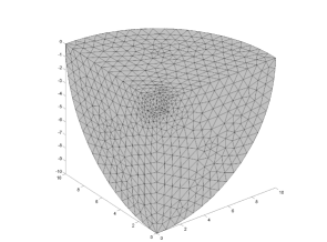
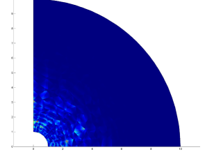
We set Ω := E 1 assign Ω subscript 𝐸 1 \Omega:=E_{1} Ω Ω \Omega u ^ = 1 / r ^ 𝑢 1 𝑟 \hat{u}=1/r ζ = 1 𝜁 1 \zeta=1 Ω R subscript Ω 𝑅 \Omega_{R} 2 1 R 𝑅 R 3 T 𝑇 T | ∇ e | 𝖫 2 ( T ) 2 superscript subscript ∇ 𝑒 superscript 𝖫 2 𝑇 2 \left|\nabla e\right|_{\operatorname{\mathsf{L}}^{2}(T)}^{2} | ∇ u ~ − v R | 𝖫 2 ( T ) 2 superscript subscript ∇ ~ 𝑢 subscript 𝑣 𝑅 superscript 𝖫 2 𝑇 2 \left|\nabla\tilde{u}-v_{R}\right|_{\operatorname{\mathsf{L}}^{2}(T)}^{2} v R subscript 𝑣 𝑅 v_{R} x 1 + x 3 = 0 subscript 𝑥 1 subscript 𝑥 3 0 x_{1}+x_{3}=0 3
Figure 2 : Ω R subscript Ω 𝑅 \Omega_{R} R = 10 𝑅 10 R=10 1 2
Table 1 : 1
Figure 3 : 1 | ∇ e | 𝖫 2 ( T ) 2 superscript subscript ∇ 𝑒 superscript 𝖫 2 𝑇 2 \left|\nabla e\right|_{\operatorname{\mathsf{L}}^{2}(T)}^{2} | ∇ u ~ − v R | 𝖫 2 ( T ) 2 superscript subscript ∇ ~ 𝑢 subscript 𝑣 𝑅 superscript 𝖫 2 𝑇 2 \left|\nabla\tilde{u}-v_{R}\right|_{\operatorname{\mathsf{L}}^{2}(T)}^{2}
The boundary value problem in step 1 of Algorithm 1 M + , R , β 2 ( ∇ u ~ , v R ) superscript subscript 𝑀 𝑅 𝛽
2 ∇ ~ 𝑢 subscript 𝑣 𝑅 M_{+,R,\beta}^{2}(\nabla\tilde{u},v_{R}) v R ∈ 𝖵 ( Ω R ) subscript 𝑣 𝑅 𝖵 subscript Ω 𝑅 v_{R}\in\operatorname{\mathsf{V}}(\Omega_{R}) v R subscript 𝑣 𝑅 v_{R} v R | S R = − ζ R − 2 e R evaluated-at subscript 𝑣 𝑅 subscript 𝑆 𝑅 𝜁 superscript 𝑅 2 superscript 𝑒 𝑅 v_{R}|_{S_{R}}=-\zeta R^{-2}e^{R} e R ⋅ v R | S R = − ζ / R 2 evaluated-at ⋅ superscript 𝑒 𝑅 subscript 𝑣 𝑅 subscript 𝑆 𝑅 𝜁 superscript 𝑅 2 e^{R}\cdot v_{R}|_{S_{R}}=-\zeta/R^{2} M − , R ( ∇ u ~ , u R ) subscript 𝑀 𝑅
∇ ~ 𝑢 subscript 𝑢 𝑅 M_{-,R}(\nabla\tilde{u},u_{R}) u R ∈ 𝖧 ∘ ( Ω R ) 1 u_{R}\in\overset{\circ}{\operatorname{\mathsf{H}}}{}^{1}(\Omega_{R}) 𝖧 ( div ) 𝖧 div \operatorname{\mathsf{H}}(\operatorname{div}) [6 ] to compute v R subscript 𝑣 𝑅 v_{R} 𝖧 1 \overset{}{\operatorname{\mathsf{H}}}{}^{1}
Example 2
We set Ω := ℝ 3 ∖ [ − 1 , 1 ] 3 assign Ω superscript ℝ 3 superscript 1 1 3 \Omega:=\mathbb{R}^{3}\setminus[-1,1]^{3} Ω Ω \Omega u ^ ^ 𝑢 \hat{u} Ω R subscript Ω 𝑅 \Omega_{R} R = 10 𝑅 10 R=10 2 1 u ~ R , 1 subscript ~ 𝑢 𝑅 1
\tilde{u}_{R,1} u ~ R , 2 subscript ~ 𝑢 𝑅 2
\tilde{u}_{R,2} 2
Table 2 : 2
These examples show that functional a posteriori error estimates
provide two-sided bounds of the error.
Of course, the accuracy depends on the method
used to generate the free variables v 𝑣 v u 𝑢 u
Acknowledgements
We heartily thank Sergey Repin for his continuous support
and the many nice and enlightening discussions.
Appendix A Appendix: Easier but Weaker Estimates
We want to point out that we can prove
a variant of Theorem 4 1 1 1 5 5 5 u ∈ 𝖧 ∘ ( Ω ) − 1 1 + { u 0 } u\in\overset{\circ}{\operatorname{\mathsf{H}}}{}^{1}_{-1}(\Omega)+\{u_{0}\}
| E | 𝖫 2 ( Ω ) , A = | ∇ u ^ − A − 1 v ~ | 𝖫 2 ( Ω ) , A ≤ | ∇ ( u ^ − u ) | 𝖫 2 ( Ω ) , A + | ∇ u − A − 1 v ~ | 𝖫 2 ( Ω ) , A , subscript 𝐸 superscript 𝖫 2 Ω 𝐴
subscript ∇ ^ 𝑢 superscript 𝐴 1 ~ 𝑣 superscript 𝖫 2 Ω 𝐴
subscript ∇ ^ 𝑢 𝑢 superscript 𝖫 2 Ω 𝐴
subscript ∇ 𝑢 superscript 𝐴 1 ~ 𝑣 superscript 𝖫 2 Ω 𝐴
\left|E\right|_{\operatorname{\mathsf{L}}^{2}(\Omega),A}=\left|\nabla\hat{u}-A^{-1}\tilde{v}\right|_{\operatorname{\mathsf{L}}^{2}(\Omega),A}\leq\left|\nabla(\hat{u}-u)\right|_{\operatorname{\mathsf{L}}^{2}(\Omega),A}+\left|\nabla u-A^{-1}\tilde{v}\right|_{\operatorname{\mathsf{L}}^{2}(\Omega),A},
and we can further estimate by Theorem 1 u ~ = u ~ 𝑢 𝑢 \tilde{u}=u v ∈ 𝖣 ( Ω ) 𝑣 absent 𝖣 Ω v\in\overset{}{\operatorname{\mathsf{D}}}(\Omega)
| E | 𝖫 2 ( Ω ) , A subscript 𝐸 superscript 𝖫 2 Ω 𝐴
\displaystyle\left|E\right|_{\operatorname{\mathsf{L}}^{2}(\Omega),A} ≤ c N , α | f + div v | 𝖫 1 2 ( Ω ) + | ∇ u − A − 1 v | 𝖫 2 ( Ω ) , A ⏟ = M + ( ∇ u , v ) + | ∇ u − A − 1 v ~ | 𝖫 2 ( Ω ) , A absent subscript ⏟ subscript 𝑐 𝑁 𝛼
subscript 𝑓 div 𝑣 subscript superscript 𝖫 2 1 Ω subscript ∇ 𝑢 superscript 𝐴 1 𝑣 superscript 𝖫 2 Ω 𝐴
absent subscript 𝑀 ∇ 𝑢 𝑣 subscript ∇ 𝑢 superscript 𝐴 1 ~ 𝑣 superscript 𝖫 2 Ω 𝐴
\displaystyle\leq\underbrace{c_{N,\alpha}\left|f+\operatorname{div}v\right|_{\operatorname{\mathsf{L}}^{2}_{1}(\Omega)}+\left|\nabla u-A^{-1}v\right|_{\operatorname{\mathsf{L}}^{2}(\Omega),A}}_{\displaystyle=M_{+}(\nabla u,v)}+\left|\nabla u-A^{-1}\tilde{v}\right|_{\operatorname{\mathsf{L}}^{2}(\Omega),A}
≤ c N , α | f + div v | 𝖫 1 2 ( Ω ) + | A − 1 ( v ~ − v ) | 𝖫 2 ( Ω ) , A ⏟ = M + ( A − 1 v ~ , v ) + 2 | ∇ u − A − 1 v ~ | 𝖫 2 ( Ω ) , A ⏟ = M ~ + ( A − 1 v ~ , ∇ u ) . absent subscript ⏟ subscript 𝑐 𝑁 𝛼
subscript 𝑓 div 𝑣 subscript superscript 𝖫 2 1 Ω subscript superscript 𝐴 1 ~ 𝑣 𝑣 superscript 𝖫 2 Ω 𝐴
absent subscript 𝑀 superscript 𝐴 1 ~ 𝑣 𝑣 2 subscript ⏟ subscript ∇ 𝑢 superscript 𝐴 1 ~ 𝑣 superscript 𝖫 2 Ω 𝐴
absent subscript ~ 𝑀 superscript 𝐴 1 ~ 𝑣 ∇ 𝑢 \displaystyle\leq\underbrace{c_{N,\alpha}\left|f+\operatorname{div}v\right|_{\operatorname{\mathsf{L}}^{2}_{1}(\Omega)}+\left|A^{-1}(\tilde{v}-v)\right|_{\operatorname{\mathsf{L}}^{2}(\Omega),A}}_{\displaystyle=M_{+}(A^{-1}\tilde{v},v)}+2\underbrace{\left|\nabla u-A^{-1}\tilde{v}\right|_{\operatorname{\mathsf{L}}^{2}(\Omega),A}}_{\displaystyle=\tilde{M}_{+}(A^{-1}\tilde{v},\nabla u)}.
Therefore, we get the same upper bound but with less good factors, i.e.,
for any θ > 0 𝜃 0 \theta>0
| E | 𝖫 2 ( Ω ) , A 2 superscript subscript 𝐸 superscript 𝖫 2 Ω 𝐴
2 \displaystyle\left|E\right|_{\operatorname{\mathsf{L}}^{2}(\Omega),A}^{2} ≤ ℳ ~ + ( v ~ ) := ( 1 + 4 / θ ) inf v ∈ 𝖣 ( Ω ) M + 2 ( A − 1 v ~ , v ) absent subscript ~ ℳ ~ 𝑣 assign 1 4 𝜃 subscript infimum 𝑣 absent 𝖣 Ω superscript subscript 𝑀 2 superscript 𝐴 1 ~ 𝑣 𝑣 \displaystyle\leq\tilde{\mathcal{M}}_{+}(\tilde{v}):=(1+4/\theta)\inf_{v\in\overset{}{\operatorname{\mathsf{D}}}(\Omega)}M_{+}^{2}(A^{-1}\tilde{v},v)
+ ( 4 + θ ) inf u ∈ 𝖧 ∘ ( Ω ) − 1 1 + { u 0 } M ~ + 2 ( A − 1 v ~ , ∇ u ) \displaystyle\qquad\qquad\qquad\qquad+(4+\theta)\inf_{u\in\overset{\circ}{\operatorname{\mathsf{H}}}{}^{1}_{-1}(\Omega)+\{u_{0}\}}\tilde{M}_{+}^{2}(A^{-1}\tilde{v},\nabla u)
with ℳ ~ + ( v ~ ) ≥ ℳ + ( v ~ ) subscript ~ ℳ ~ 𝑣 subscript ℳ ~ 𝑣 \tilde{\mathcal{M}}_{+}(\tilde{v})\geq\mathcal{M}_{+}(\tilde{v}) θ = 1 𝜃 1 \theta=1 1 + 4 / θ = 4 + θ = 5 1 4 𝜃 4 𝜃 5 1+4/\theta=4+\theta=5 ℳ ~ + ( v ~ ) = 5 ℳ + ( v ~ ) subscript ~ ℳ ~ 𝑣 5 subscript ℳ ~ 𝑣 \tilde{\mathcal{M}}_{+}(\tilde{v})=5\mathcal{M}_{+}(\tilde{v}) u ∈ 𝖧 ∘ ( Ω ) − 1 1 u\in\overset{\circ}{\operatorname{\mathsf{H}}}{}^{1}_{-1}(\Omega)
| E | 𝖫 2 ( Ω ) , A 2 superscript subscript 𝐸 superscript 𝖫 2 Ω 𝐴
2 \displaystyle\left|E\right|_{\operatorname{\mathsf{L}}^{2}(\Omega),A}^{2} = | ∇ u ^ − A − 1 v ~ | 𝖫 2 ( Ω ) , A 2 absent superscript subscript ∇ ^ 𝑢 superscript 𝐴 1 ~ 𝑣 superscript 𝖫 2 Ω 𝐴
2 \displaystyle=\left|\nabla\hat{u}-A^{-1}\tilde{v}\right|_{\operatorname{\mathsf{L}}^{2}(\Omega),A}^{2}
≥ 2 ⟨ ∇ u ^ − A − 1 v ~ , ∇ u ⟩ 𝖫 2 ( Ω ) , A − | ∇ u | 𝖫 2 ( Ω ) , A 2 absent 2 subscript ∇ ^ 𝑢 superscript 𝐴 1 ~ 𝑣 ∇ 𝑢
superscript 𝖫 2 Ω 𝐴
superscript subscript ∇ 𝑢 superscript 𝖫 2 Ω 𝐴
2 \displaystyle\geq 2\left\langle\nabla\hat{u}-A^{-1}\tilde{v},\nabla u\right\rangle_{\operatorname{\mathsf{L}}^{2}(\Omega),A}-\left|\nabla u\right|_{\operatorname{\mathsf{L}}^{2}(\Omega),A}^{2}
= 2 ⟨ f , u ⟩ 𝖫 2 ( Ω ) − ⟨ ∇ u + 2 A − 1 v ~ , ∇ u ⟩ 𝖫 2 ( Ω ) , A = M − ( A − 1 v ~ , u ) absent 2 subscript 𝑓 𝑢
superscript 𝖫 2 Ω subscript ∇ 𝑢 2 superscript 𝐴 1 ~ 𝑣 ∇ 𝑢
superscript 𝖫 2 Ω 𝐴
subscript 𝑀 superscript 𝐴 1 ~ 𝑣 𝑢 \displaystyle=2\left\langle f,u\right\rangle_{\operatorname{\mathsf{L}}^{2}(\Omega)}-\left\langle\nabla u+2A^{-1}\tilde{v},\nabla u\right\rangle_{\operatorname{\mathsf{L}}^{2}(\Omega),A}=M_{-}(A^{-1}\tilde{v},u)
and the additional term M ~ − ( A − 1 v ~ , A − 1 v , ∇ u ) subscript ~ 𝑀 superscript 𝐴 1 ~ 𝑣 superscript 𝐴 1 𝑣 ∇ 𝑢 \tilde{M}_{-}(A^{-1}\tilde{v},A^{-1}v,\nabla u)
| E | 𝖫 2 ( Ω ) , A 2 ≥ ℳ ~ − ( v ~ ) := sup u ∈ 𝖧 ∘ ( Ω ) − 1 1 M − ( A − 1 v ~ , u ) \left|E\right|_{\operatorname{\mathsf{L}}^{2}(\Omega),A}^{2}\geq\tilde{\mathcal{M}}_{-}(\tilde{v}):=\sup_{u\in\overset{\circ}{\operatorname{\mathsf{H}}}{}^{1}_{-1}(\Omega)}M_{-}(A^{-1}\tilde{v},u)
with ℳ ~ − ( v ~ ) ≤ ℳ − ( v ~ ) subscript ~ ℳ ~ 𝑣 subscript ℳ ~ 𝑣 \tilde{\mathcal{M}}_{-}(\tilde{v})\leq\mathcal{M}_{-}(\tilde{v})