Obvious natural morphisms of sheaves are unique

Abstract

We prove that a large class of natural transformations (consisting roughly of those constructed via composition from the “functorial” or “base change” transformations) between two functors of the form $\cdots f^{*}g_{*}\cdots$ actually has only one element, and thus that any diagram of such maps necessarily commutes. We identify the precise axioms defining what we call a “geofibered category” that ensure that such a coherence theorem exists. Our results apply to all the usual sheaf-theoretic contexts of algebraic geometry. The analogous result that would include any other of the six functors remains unknown.

Commutative diagrams express one of the most typical subtle beauties of mathematics, namely that a single object (in this case an arrow in some category) can be realized by several independent constructions. The more interesting the constructions, the more insight is gained by carefully verifying commutativity, and it is tempting to take the inverse claim to mean that comparable arrows, constructed mundanely, should be expected to be equal and are therefore barely worth proving to be so. As half the purpose of a human-produced publication is to provide insight, there is some validity in thinking that any opportunity to reduce both length and tedium is worth taking, but this is at odds with the other half, which is to supply rigor. The goal of this paper is, therefore, to serve both ends by proving that a large class of diagrams commonly encountered in algebraic geometry, obtained from the fibered category nature of sheaves, are both interesting and necessarily commutative.

The goal of proving “all diagrams commute” began with the first “coherence theorem” of this kind, proved by Mac Lane [maclane]; further research, apparently, has not yet developed this particular application, as we are not aware of any coherence theorems that apply to fibered categories. Indeed, our main result LABEL:main_theorem is itself not entirely free of conditions, and our best unconditional result such as in LABEL:secondary_theorem is somewhat restricted in scope. A similar statement to the latter was obtained by Jacob Lurie [lurie] concerning arbitrary tensor isomorphisms of functors on coherent sheaves over a stack; ours applies to less general morphisms but more general situations. The problem of proving a general coherence theorem for pullbacks and pushforwards in the context of monoidal functors was mentioned in Fausk–Hu–May [fausk-may] and said to be both unsolved and desirable; we do not claim to have solved it, though certainly, we have done something. Those authors do not consider multiple maps $f$ in combination, however, as we do.

The goal of rigoriously verifying the diagrams of algebraic geometry has been pursued by several people, notably recently Brian Conrad in [conrad], who proved the compatibility of the trace map of Grothendieck duality with base change. Our theorems do not seem to apply to this problem, most significantly because almost every construction in that book intimately refers to details of abelian and derived categories and to methods of homological algebra, none of which are addressed here. Such a quality is possessed by many constructions of algebraic geometry and place many of its interesting compatibilities potentially out of reach of the results stated here.

Maps constructed in such a way, as concerns Conrad constantly in that book, can certainly differ by a natural sign, if not worse, and so the only hope for automatically proving commutativity of that kind of diagram is to separate the cohomological part from the categorical part and apply our results only to the latter. This is to say nothing of the explicit avoidance of “good” hypotheses (for example, flatness, such as we will consider) on the schemes and morphisms considered there, all of which place this particular compatibility on the other side of the line separating “interesting” from “mundane”.

In 1, we give (many) definitions in preparation for stating the main theorems; comments on the hypotheses considered there are given in 7, as are the acknowledgements. These theorems are given, without proof, in 2, and their proofs are delayed until 6. The style of these first two sections of this paper is quite formal; for a more relaxed overview, see A. 3 quickly presents our use of “string diagrams”, a computational tool we will use to give structure to some of our more arbitrary calculations; further details and comparison with others’ use of this tool is given in B. Afterwards, Sections 4 and 5 contain the core arguments upon which the eventual high-level proofs rely.

1 Definitions and notation

In this section we define the natural transformations we consider and will eventually prove are unique. Since they apply to a variety of similar but slightly different common situations in algebraic geometry, we have abstracted the essential properties into a formal object of category theory; the particular applications are indicated in 2.

Abstract push and pull functors.

Our results apply in a variety of similar situations with slightly different features and technical hypotheses, all unified by the formalism of pushforward and pullback. The following definition encapsulates the axiomatic properties we will require.

Theorem 1.1.

defngeofibered category We define a geofibered category to be a functor $F\colon\mathbf{Sh}\to\mathbf{Sp}$ between two categories called, respectively, “shapes” and “spaces”, such that:

• The category $\mathbf{Sp}$ has all finite fibered products.

• For every morphism $f\colon X\to Y$ of $\mathbf{Sp}$, there are functors

  $$f^{*}\colon\mathbf{Sh}_{Y}\longleftrightarrow\mathbf{Sh}_{X}:f_{*}$$

  between the fibers over $Y$ and $X$, which are an adjoint pair $(f^{*},f_{*})$.

• The assignment $X\mapsto\mathbf{Sh}_{X}$ and $f\mapsto f^{*}$ constitutes a pseudofunctor $\mathbf{Sp}\to\mathbf{Cat}$; i.e. a cleaved fibered category, as described below.

• Dually, the assignment $X\mapsto\mathbf{Sh}_{X}$ and $f\mapsto f_{*}$ constitutes a pseudofunctor $\mathbf{Sp}\to\mathbf{Cat}^{\mathrm{op}}$.

• The above pseudofunctor data obey the compatibilities described in the remainder of this subsection.

The terminology was chosen in part because “bifibered category” has a different meaning, and also to indicate that this concept models the fibered category of sheaves in various geometries. For a description of pseudofunctors in the context of fibered categories, see Vistoli’s exposition [vistoli]*§3.1.2.

The requirement that $\mathbf{Sp}$ has fibered products is only strictly speaking necessary for some of the following definitions, but since that of the “roof” is among them, given the central nature of this concept in our main theorems, a geofibered category would be quite useless otherwise.

The rest of this subsection is devoted to introducing notation and terminology and, along side it, describing the compatibilities of the data of a geofibered category.

Theorem 1.2.

defnSGFs As per LABEL:geofibered_category, in any geofibered category, for any morphism $f\colon X\to Y$ of spaces we have adjoint functors $(f^{*},f_{*})$ of shapes which we call basic standard geometric functors (the terminology intentionally references “geometric morphisms” of topoi)

We define a standard geometric functor (SGF) to be any composition of basic standard geometric functors. Formally, an SGF is equivalent to a diagram of spaces and morphisms forming a directed graph that is topologically linear, together with an ordering of its vertices from one end of the segment to the other (i.e. we “remember” the terms of the composition as well as the resulting functor). For an SGF $F$ from shapes on $X$ to shapes on $Y$, we write $X=\operatorname{S}(F)$ and $Y=\operatorname{T}(F)$.

The pseudofunctor data consists of a number of natural transformations, which are the basis for the main objects of our study.

Theorem 1.3.

defnbasic SGNTs Between pairs of SGFs there are canonical natural transformations of the following three types that we call the basic standard geometric natural transformations:

$$\left.\begin{aligned} \operatorname{\mathsf{unit}}(f)&\colon\operatorname{id}\to f_{*}f^{*}\\ \operatorname{\mathsf{counit}}(f)&\colon f^{*}f_{*}\to\operatorname{id}\end{aligned}\right\}$$ Adjunctions (1.1a)

$$\left.\begin{aligned} \operatorname{\mathsf{comp}}^{*}(f,g)&\colon f^{*}g^{*}\xrightarrow{\sim}(gf)^{*}\\ \operatorname{\mathsf{comp}}_{*}(f,g)&\colon g_{*}f_{*}\xrightarrow{\sim}(gf)_{*}\end{aligned}\right\}$$ Compositions (1.1b)

$$\left.\begin{aligned} \operatorname{\mathsf{triv}}_{*}(f)&\colon\mathrm{id}_{*}\xrightarrow{\sim}\mathrm{id}\\ \operatorname{\mathsf{triv}}^{*}(f)&\colon\mathrm{id}^{*}\xrightarrow{\sim}\mathrm{id}\end{aligned}\right\} \text{\emph{Trivializations}}.$$ (1.1c)

For the latter two types, we will use ^-1 to denote their inverses (which will not arise as often in our arguments).

The origins, nature, and compatibilities of these transformations are described in the following subpoints.

Adjunctions.

The maps $\operatorname{\mathsf{unit}}(f)$ and $\operatorname{\mathsf{counit}}(f)$ are equivalent to the $(f^{*},f_{*})$ adjunction in the usual way and satisfy the familiar compatibility required of an adjunction, which we state at risk of being pedantic so as to provide a complete reference for the data of a geofibered category.

$$\bigl{(}f^{*}\xrightarrow{f^{*}\operatorname{\mathsf{unit}}(f)} f^{*}f_{*}f^{*}\xrightarrow{\operatorname{\mathsf{counit}}(f)f^{*}}f^{*}\bigr{)} =\mathrm{id}$$ (1.2a)

$$\bigl{(}f_{*}\xrightarrow{\operatorname{\mathsf{unit}}(f)f_{*}} f_{*}f^{*}f_{*}\xrightarrow{f_{*}\operatorname{\mathsf{counit}}(f)}f_{*}\bigr{)} =\mathrm{id}$$ (1.2b)

In the context of natural transformations of functors rather than morphisms of individual objects, we have a “reverse natural adjunction” also defined by the unit and counit; we use it on occasion to aid definitions. The construction and proof of bijectivity are left as an exercise for readers who desire it.

$$\operatorname{\mathsf{RNA}}_{f}\colon\operatorname{Hom}(Ff_{*},G)\longleftrightarrow\operatorname{Hom}(F,Gf^{*}).$$ (1.3)

Compositions.

The data of a pseudofunctor implies the existence of isomorphisms $\operatorname{\mathsf{comp}}_{*}(f,g)\colon(fg)_{*}\cong f_{*}g_{*}$ for every composable pair of morphisms $f,g$ of spaces. Likewise, we have isomorphisms $\operatorname{\mathsf{comp}}^{*}(f,g)\colon(fg)^{*}\cong g^{*}f^{*}$. The compatibilities required of these data by a pseudofunctor express their associativity in triple compositions:

$$\bigl{(}(fgh)_{*}\cong(fg)_{*}h_{*}\cong f_{*}g_{*}h_{*}\bigr{)}=\bigl{(}(fgh)_{*}\cong f_{*}(gh)_{*}\cong f_{*}g_{*}h_{*}\bigr{)}$$ (1.4)

and similarly for pullbacks. It must be noted that this data for pushforwards or pullbacks alone determines such data for the other; for example, given pseudofunctoriality of $f_{*}$, for the adjoint $f^{*}$, we define $\operatorname{\mathsf{comp}}^{*}(f,g)$ via category-theoretic formalism: $(fg)_{*}$ has the left adjoint $(fg)^{*}$ and the composition $f_{*}g_{*}$ has as left adjoint the composition $g^{*}f^{*}$; since we have $(fg)_{*}\cong f_{*}g_{*}$ we also get $(fg)^{*}\cong g^{*}f^{*}$ by uniqueness of left adjoints. In more explicit terms, this means that for any shapes $\mathcal{F}$ and $\mathcal{G}$, we have an isomorphism

$$\operatorname{Hom}((fg)^{*}\mathcal{F},\mathcal{G})\cong\operatorname{Hom}(\mathcal{F},(fg)_{*}\mathcal{G})\cong\operatorname{Hom}(\mathcal{F},f_{*}g_{*}\mathcal{G})\cong\operatorname{Hom}(f^{*}\mathcal{F},g_{*}\mathcal{G})\\ \cong\operatorname{Hom}(g^{*}f^{*}\mathcal{F},\mathcal{G}).$$ (1.5)

We require as a compatibility relation that this is $\operatorname{Hom}(\operatorname{\mathsf{comp}}^{*}(f,g)_{\mathcal{F}},\mathcal{G})$.

Trivializations.

The trivialization isomorphism $\operatorname{\mathsf{triv}}_{*}\colon\mathrm{id}_{*}\cong\mathrm{id}$ is another part of the pseudofunctor data (and likewise for pullbacks), as well as its compatibility with composition:

$$\bigl{(}\operatorname{\mathsf{comp}}_{*}(\mathrm{id},f)\colon\mathrm{id}_{*}f_{*}\cong(\mathrm{id}f)_{*}=f_{*}\bigr{)}=\bigl{(}\operatorname{\mathsf{triv}}_{*}f_{*}\colon\mathrm{id}_{*}f_{*}\cong\mathrm{id}f_{*}=f_{*}\bigr{)}$$ (1.6)

(and, again, the same for pullbacks). Given this data just for pullbacks or pushforwards, for example the latter, we could define an isomorphism $\mathrm{id}^{*}\to\mathrm{id}$ and its inverse by adjunction, similar to 1.5:

$$\operatorname{Hom}(\mathrm{id}^{*}\mathcal{F},\mathcal{G})\cong\operatorname{Hom}(\mathcal{F},\mathrm{id}_{*}\mathcal{G})\cong\operatorname{Hom}(\mathcal{F},\mathcal{G}).$$ (1.7)

We require that this isomorphism be equal to $\operatorname{Hom}(\operatorname{\mathsf{triv}}^{*}_{\mathcal{F}},\mathcal{G})$.

Classes of transformations.

Typically we do not consider transformations in the pure form above, but rather in horizontal composition with some identity maps.

Basic classes.

The following are the classes of natural transformations consisting of just one of the basic ones in horizontal composition.

Theorem 1.4.

defnbasic SGNT classes In this definition, $F$ and $G$ represent any SGFs; $f$ and $g$ represent any maps of spaces. We define:

$$\operatorname{\mathsf{unit}} =\{F\operatorname{\mathsf{unit}}(f)G\} \operatorname{\mathsf{counit}} =\{F\operatorname{\mathsf{counit}}(f)G\}$$ (1.8a)

$$\operatorname{\mathsf{comp}}_{0} =\{F\operatorname{\mathsf{comp}}_{*}(f,g)G\}\cup\{F\operatorname{\mathsf{comp}}^{*}(f,g)G\} \operatorname{\mathsf{comp}} =\operatorname{\mathsf{comp}}_{0}\cup\operatorname{\mathsf{comp}}_{0}^{-1}$$ (1.8b)

$$\operatorname{\mathsf{triv}}_{0} =\{F\operatorname{\mathsf{triv}}_{*}G\}\cup\{F\operatorname{\mathsf{triv}}^{*}G\} \operatorname{\mathsf{triv}} =\operatorname{\mathsf{triv}}_{0}\cup\operatorname{\mathsf{triv}}_{0}^{-1}.$$ (1.8c)

And now we may introduce the main objects of our study.

Theorem 1.5.

defnSGNTs A standard geometric natural transformation (SGNT) is an element of the class (in which we use the notation $\langle S\rangle$ to denote the class generated by $S$ via composition)

$$\operatorname{\mathsf{SGNT}}=\langle\operatorname{\mathsf{unit}}\cup\operatorname{\mathsf{counit}}\cup\operatorname{\mathsf{comp}}\cup\operatorname{\mathsf{triv}}\rangle.$$ (1.9)

For any SGNT $\phi\colon F\to G$ between two SGFs, we write $F=\operatorname{dom}\phi$ and $G=\operatorname{cod}\phi$.

Another way of understanding this class is the following characterization: $\operatorname{\mathsf{SGNT}}$ is the smallest category of natural transformations of SGFs containing all identity maps, $\operatorname{\mathsf{comp}}$ maps, $\operatorname{\mathsf{triv}}$ maps, and their inverses, and that is closed under horizontal and vertical composition and adjunction of ^∗ and _∗.

The following type of SGNT is of fundamental importance throughout the paper; it arises seemingly of its own accord in a variety of situations and is also essential in simplifying SGFs to the point that our main theorem is provable.

Theorem 1.6.

defncommutative diagram morphism Consider a commutative diagram

(1.10)

We define the associated commutation morphism

$$\operatorname{\mathsf{cd}}(f,g;\tilde{f},\tilde{g})\colon g^{*}f_{*}\to\tilde{f}_{*}\tilde{g}^{*}$$ (1.11)

to be the map corresponding by $g$-adjunction and $\tilde{g}$- reverse natural adjunction to the corner-swapping map

$$f_{*}\tilde{g}_{*}\xrightarrow{\operatorname{\mathsf{comp}}_{*}(\tilde{g},f)}(f\tilde{g})_{*}=(g\tilde{f}_{*})\xrightarrow{\operatorname{\mathsf{comp}}_{*}(\tilde{f},g)^{-1}}g_{*}\tilde{f}_{*}$$ (1.12)

See 4.6 for a visualization of this definition.

The commutation morphisms are too general to be entirely useful, though it is helpful to retain the concept for manipulations when no further hypotheses are needed. Nonetheless, for our theorems such hypotheses are needed.

Theorem 1.7.

defnbase change morphism When 1.10 is cartesian, we write $\operatorname{\mathsf{bc}}(f,g)=\operatorname{\mathsf{cd}}(f,g;\tilde{f},\tilde{g})$ and use the aggregate notation, as before:

$$\operatorname{\mathsf{bc}}=\{F\operatorname{\mathsf{bc}}(f,g)G\}.$$ (1.13)

Invertible base changes.

In this subsection and the next, we introduce some further conditions on geofibered categories that support a larger class of natural transformations to which to apply our theorems. We include the proofs of a few of their simplest properties, some of which are necessary for the definitions to make sense and others are simply most appropriate when placed here.

We begin with an abstract structure on geofibered categories inspired by LABEL:base_change_morphism.

Theorem 1.8.

defngeolocalizing Let $\mathbf{Sh}\to\mathbf{Sp}$ be a geofibered category. We will call a class $P$ of morphisms in $\mathbf{Sp}$ push-geolocalizing if:

• It contains every isomorphism and is closed under composition.

• For each $f\in P$ and $g\in\mathbf{Sp}$, the base change $\operatorname{\mathsf{bc}}(f,g)$ is an isomorphism and $\tilde{f}\in P$.

Similarly, we define $P$ to be pull-geolocalizing by swapping the roles of $f$ and $g$. We say that a geofibered category is given a geolocalizing structure if it is equipped with a pair of push- and pull-geolocalizing classes in $\mathbf{Sp}$.

We chose the word “localizing” in deference to the convention that to invert morphisms of a category is to localize it; the full term “geolocalizing” is in part to complement “geofibered”, and in part to indicate that it is not the geolocalizing morphisms themselves that are inverted.

We note that, by definition, every geofibered category has a “trivial” geolocalizing structure consisting of just the isomorphisms of $\mathbf{Sp}$.

This concept matched by that of a “good” SGF or SGNT, based on the following concept. Its uniqueness claim will be proven later, to keep this section efficient.

Theorem 1.9.

defnalternating We say that an SGF $F$ is alternating if it is of the form $(f_{*})g^{*}h_{*}\cdots$ ($f$ optional), where none of $f$, $g$, $h$, $\dots$ is the identity map. The alternating reduction of $F$ is the unique (by LABEL:alternating_unique) alternating SGF $F^{\prime}$ admitting an SGNT in $\langle\operatorname{\mathsf{comp}}_{0}\cup\operatorname{\mathsf{triv}}_{0}\rangle$ (thus, an isomorphism in $\operatorname{\mathsf{SGNT}}$) $F\to F^{\prime}$.

Theorem 1.10.

defngood Let $\mathbf{Sh}\to\mathbf{Sp}$ be a geolocalizing geofibered category, and let $F$ be an alternating SGF; we say that it is good if, either: every basic SGF in $F$ of the form $f^{*}$ is pull-geolocalizing; or, every basic SGF in $F$ of the form $f_{*}$ is push-geolocalizing. For any SGF, we say that it is good if it has a good alternating reduction. We say that an SGNT $\phi\colon F\to G$ is good if both $F$ and $G$ are good.

Theorem 1.11.

lemgood persistence If $F$ is good, then for any SGNT $\phi\colon F\to G$ with $\phi\in\operatorname{\mathsf{comp}}\cup\operatorname{\mathsf{triv}}$, we have $G$ good as well. If $F$ is alternating, the same is true for $\phi\in\operatorname{\mathsf{bc}}$.

Proof 1.12.

Let $\alpha\colon F\to F^{\prime}$ and $\beta\colon G\to G^{\prime}$ be the alternating reductions of $F$ and $G$. If $\phi\in\operatorname{\mathsf{comp}}_{0}\cup\operatorname{\mathsf{triv}}_{0}$, then $\beta\phi$ is also an alternating reduction of $F$, and thus by LABEL:alternating we have $F^{\prime}=G^{\prime}$; since $F$ (and thus $F^{\prime}$) is good by hypothesis, $G^{\prime}$ (and thus $G$) is good. Likewise, if $\phi\in\operatorname{\mathsf{comp}}_{0}^{-1}\cup\operatorname{\mathsf{triv}}_{0}^{-1}$, then $\alpha\phi^{-1}$ is an alternating reduction of $G$ and so we have $G^{\prime}=F^{\prime}$ and thus, again, that $G$ is good.

Finally, for $\phi\in\operatorname{\mathsf{bc}}$, it is clear first of all that for a map $\operatorname{\mathsf{bc}}(f,g)\colon g^{*}f_{*}\to\tilde{f}_{*}\tilde{g}^{*}$ itself, the right-hand side is good if the left is, because the hypotheses imposed by goodness on the maps of spaces are stable under base change. For a more general element $A\operatorname{\mathsf{bc}}(f,g)B$ of $\operatorname{\mathsf{bc}}$, if $F=Ag^{*}f_{*}B$ is good and alternating then $G=A\tilde{f}_{*}\tilde{g}^{*}B$ satisfies the conditions given in LABEL:good (but is not alternating); since the (push-, pull-) geolocalizing morphisms are closed under composition and contain the identity, these conditions are preserved by passage through any element of $\langle\operatorname{\mathsf{comp}}_{0}\cup\operatorname{\mathsf{triv}}_{0}\rangle$, so the same conditions are satisfied by the alternating reduction $G^{\prime}$; i.e. $G^{\prime}$, hence $G$, is good.

This definition is complemented and completed by the following concept, upon which all significant results of this paper are ultimately based.

Theorem 1.13.

defnroof Let $\mathbf{Sh}\to\mathbf{Sp}$ be a geofibered category and let $F$ be any SGF, viewed as a diagram of morphisms in $\mathbf{Sp}$. We define the roof of $F$, denoted $\operatorname{roof}(F)$, by constructing the final object in the category of spaces with maps to this diagram, which exists and is unique by the universal property of the fibered product.

Then the roof is the space thus defined, also denoted $\operatorname{roof}(F)$, together with its “projection” morphisms

$$a_{F}\colon\operatorname{roof}(F)\to\operatorname{T}(F) b_{F}\colon\operatorname{roof}(F)\to\operatorname{S}(F).$$ (1.14)

We also define $\operatorname{roof}(F)$ as an SGF to be the functor $a_{F{*}}b_{F}^{*}$ (resp. $a_{F{*}}$ if $b_{F}=\mathrm{id}$, resp. $b_{F}^{*}$ if $a_{F}=\mathrm{id}$, resp. $\mathrm{id}$), and in LABEL:roof_morphism we will construct a canonical SGNT $F\to\operatorname{roof}(F)$ that we will also call $\operatorname{roof}(F)$. We will make an effort to eliminate ambiguity.

Just as for goodness, the concept of a roof comes associated with a natural morphism. We state this proposition here and prove it as Propositions LABEL:roof_morphism_uniqueness and LABEL:roof_morphism_construction.

Theorem 1.14.

proproof morphism For any SGF $F$, its roof is the unique SGF of the form $a_{*}b^{*}$ admitting admitting a map $\operatorname{roof}(F)\colon F\to\operatorname{roof}(F)$ in $\operatorname{\mathsf{SGNT}}_{0}^{+}$. This map exists and is uniquely determined by the properties that it factors through the alternating reduction of $F$ and, if $F$ is alternating, through an element of $\operatorname{\mathsf{bc}}$.

Theorem 1.15.

corroof isomorphism Let $\mathbf{Sh}\to\mathbf{Sp}$ be a geolocalizing geofibered category. If $F$ is any good SGF, then $\operatorname{roof}(F)$ is also good, and $\operatorname{roof}(F)\colon F\to\operatorname{roof}(F)$ is a natural isomorphism.

Proof 1.16.

In the construction of LABEL:roof_morphism, the roof morphism is constructed in such a way that its factors in $\operatorname{\mathsf{bc}}$ are applied only to an alternating source, with the other factors in $\operatorname{\mathsf{comp}}_{0}$ or $\operatorname{\mathsf{triv}}_{0}$ by LABEL:alternating. Therefore LABEL:good_persistence applies and each composand of $\operatorname{roof}(F)$ is good. Then each base-change factor is, by definition of good, an isomorphism, while all the other factors are automatically so.

This motivates notation for classes of SGNTs including the inverses of invertible base changes.

Theorem 1.17.

defninvertible base changes We use the following class notation for the “balanced” elements of $\operatorname{\mathsf{SGNT}}$ in which the units and counits only occur in pairs within a base change morphism, along with a “forward” variant:

$$\operatorname{\mathsf{SGNT}}_{0}^{+}=\langle\operatorname{\mathsf{bc}}\cup\operatorname{\mathsf{comp}}_{0}\cup\operatorname{\mathsf{triv}}_{0}\rangle \operatorname{\mathsf{SGNT}}_{0}=\langle\operatorname{\mathsf{SGNT}}_{0}^{+}\cup(\operatorname{\mathsf{SGNT}}_{0}^{+})^{-1}\rangle.$$ (1.15)

Here we use the inverse notation to refer to the class of inverses of only the actually invertible (as abstract natural transformations) elements of $\operatorname{\mathsf{SGNT}}_{0}^{+}$.

Invertible unit morphisms.

We will also be allowing the inverses of certain units and counits, whose definition is more technical. The goodness hypothesis in this next definition is, strictly speaking, unnecessary for its formulation, but as it is required in our only nontrivial example of this concept, LABEL:etale_acyclicity, it seems likely that without it the definition would be invalid.

Theorem 1.18.

defnacyclicity structure Let $\mathbf{Sh}\to\mathbf{Sp}$ be a geolocalizing geofibered category. We define an acyclicity structure on it to be a class $C$ of pairs $(a,b)$ of morphisms of $\mathbf{Sp}$ having the properties:

• Every pair $(a,i)$ or $(i,b)$, with $a$ being push-geolocalizing and $b$ being pull-geolocalizing, and where $i$ is any invertible morphism in $\mathbf{Sp}$ (and having the appropriate sources and targets, as below), is in $C$.

• For any $(a,b)\in C$, we have $\operatorname{S}(a_{*})=\operatorname{T}(b^{*})$, and for every $f\in\mathbf{Sp}$ such that $a_{*}\operatorname{\mathsf{unit}}(f)b^{*}$ is good and a natural isomorphism, either (left invertibility) $a_{*}\operatorname{\mathsf{unit}}(f)$, or (right invertibility) $\operatorname{\mathsf{unit}}(f)b^{*}$ is a natural isomorphism.

• $C$ is closed under base change in the following sense: for any pair of maps $X\to\operatorname{T}(a_{*})$ and $Y\to\operatorname{S}(b^{*})$, the base change

  $$(\tilde{a},\tilde{b})=X\times_{\operatorname{T}(a_{*})}(a,b)\times_{\operatorname{S}(b^{*})}Y$$ (1.16)

  of the pair map $(a,b)$ into $\operatorname{T}(a_{*})\times\operatorname{S}(b^{*})$ is in $C$.

This entails the derived concept of admissibility: an SGF $F$ is admissible if $\operatorname{roof}(F)=(a_{F},b_{F})$ is in $C$. We will say, correspondingly, that any $(a,b)\in C$ is itself admissible.

We chose “acyclicity structure” in reference to a morphism $f\colon X\to Y$ being acyclic in geometry or topology when $\operatorname{\mathsf{unit}}(f)$ is an isomorphism on certain sheaves (e.g. possibly only those of the form $b^{*}\mathcal{F}$), potentially after taking cohomology (i.e. applying derived $a_{*}$).

We note that, by definition, every geolocalizing geofibered category has a “trivial” acyclicity structure consisting of just the pairs $(a,i)$ and $(i,b)$ of the first point.

Theorem 1.19.

defninvertible units Let $\mathbf{Sh}\to\mathbf{Sp}$ be a geolocalizing geofibered category with acyclicity structure. We define the class $\operatorname{\mathsf{Unit}}$ to be the class of all good SGNTs of the form $F\phi G$, where $\phi=A\operatorname{\mathsf{unit}}(f)B$ is a natural isomorphism and $\operatorname{dom}(\phi)$ (which is $AB$) is admissible.

Until now we have ignored the counits, but for the most part, this is justifiable. We give the proof of the following lemma in 6.

Theorem 1.20.

lemcounits auxiliary We have $\operatorname{\mathsf{counit}}\subset\langle\operatorname{\mathsf{SGNT}}_{0}^{+}\cup\operatorname{\mathsf{unit}}\rangle$ and, with $\operatorname{\mathsf{Counit}}$ as in LABEL:invertible_units but with good $\operatorname{\mathsf{counit}}(f)$ replacing arbtrary $\operatorname{\mathsf{unit}}(f)$, we have $\operatorname{\mathsf{Counit}}\subset\langle\operatorname{\mathsf{SGNT}}_{0}^{+}\cup\operatorname{\mathsf{Unit}}\rangle$.

2 Main theorems

In this section we suppose the existence of an ambient geolocalizing geofibered category with an acyclicity structure, $\mathbf{Sh}\to\mathbf{Sp}$; as we have noted, any geofibered category can play this role with trivial structures; among our results is a description of some nontrivial ones. Our main results are of two types: the first contains a “quantitative” and comparatively technical result on SGNTs; the second contains a “qualitative” corollary. Proofs, if not indicated otherwise, are given in 6.

The quantitative result is a classification of SGNTs:

Theorem 2.1.

thmSGNT0 inverses square Let $\phi\colon F\to G$ be in $\langle\operatorname{\mathsf{SGNT}}\cup\operatorname{\mathsf{bc}}^{-1}\cup\operatorname{\mathsf{Unit}}^{-1}\rangle$, and denote $\operatorname{roof}(G)=a_{G{*}}b_{G}^{*}$. Then there exist maps of spaces $f$ and $g$, such that $a_{G{*}}\operatorname{\mathsf{unit}}(g)b_{G}^{*}$ is a natural isomorphism, forming a commutative diagram:

(2.1)

The upward arrow can be omitted for $\phi\in\langle\operatorname{\mathsf{SGNT}}\cup\operatorname{\mathsf{bc}}^{-1}\rangle$.

The last sentence is LABEL:SGNT0_square, and the rest is LABEL:SGNT0_inverses_square'. The use of $\langle\operatorname{\mathsf{SGNT}}\cup\operatorname{\mathsf{bc}}^{-1}\rangle$ rather than $\langle\operatorname{\mathsf{SGNT}}_{0}\cup\operatorname{\mathsf{unit}}\rangle$ is justified by LABEL:counits_auxiliary.

Now we give criteria under which “all diagrams commute”; i.e. there exists only one SGNT between two given SGFs. First, we have the basic Corollaries LABEL:big_alternating_unique and LABEL:SGNT0_roofs:

Theorem 2.2.

thmbasic theorem

1. For any SGFs $F$ and $G$, there exists at most one $\phi\colon F\to G$ in $\langle\operatorname{\mathsf{comp}}\cup\operatorname{\mathsf{triv}}\rangle$.

2. Let $G=a_{*}b^{*}$; then for any SGF $F$, there exists at most one $\phi\colon F\to G$ in $\operatorname{\mathsf{SGNT}}_{0}$.

We have also found a curious conclusion that is not quite a corollary of the latter nor of the main theorem:

Theorem 2.3.

thmsecondary theorem Let $\phi\colon F\to G$ be in $\operatorname{\mathsf{SGNT}}$, where both $F$ and $G$ have at most one basic SGF. Then either both are trivial and $\phi\in\operatorname{\mathsf{triv}}_{0}^{-1}\operatorname{\mathsf{triv}}_{0}$, or neither is, so $F=G$ and $\phi=\mathrm{id}$.

More importantly, we have the following general theorem:

Theorem 2.4.

thmmain theorem Let $\phi\colon F\to G$ be a natural transformation of SGFs.

Write $\operatorname{S}(F)=\operatorname{S}(G)=X$ and $\operatorname{T}(F)=\operatorname{T}(G)=Y$; denote $Z=X\times Y$ and let $b\colon\operatorname{roof}(F)\times_{Z}\operatorname{roof}(G)\to\operatorname{roof}(G)$ be the projection map, where $\operatorname{roof}(F)\to Z$ and $\operatorname{roof}(G)\to Z$ are the pair maps $(b_{F},a_{F})$ and $(b_{G},a_{G})$; suppose that the unit map $a_{G{*}}\operatorname{\mathsf{unit}}(b)b_{G}^{*}$ is an isomorphism.

Suppose as well that the map $\operatorname{roof}(G)\colon G\to\operatorname{roof}(G)$ is an isomorphism. If $\phi\in\langle\operatorname{\mathsf{SGNT}}\cup\operatorname{\mathsf{bc}}^{-1}\cup\operatorname{\mathsf{Unit}}^{-1}\rangle$, then it is the unique map $\psi\colon F\to G$ in that class.

We also have an auxiliary lemma giving sufficient conditions for the hypotheses of the theorem to hold. To state it, we use the term weakly admissible of an SGF $F$ to mean that the pair morphism $(a_{F},b_{F})$ of its roof is a universal monomorphism.

Theorem 2.5.

lemconditions auxiliary We have $\operatorname{roof}(G)$ is an isomorphism if $G$ is good. The other condition of LABEL:main_theorem holds if either:

• $F$ is weakly admissible, and either there exists some $\phi\in\langle\operatorname{\mathsf{SGNT}}_{0}\cup\operatorname{\mathsf{unit}}\rangle$, or its consequence: $(b_{G},a_{G})$ factors through $(b_{F},a_{F})$;

• $G$ is weakly admissible and there exists some $\phi\in\langle\operatorname{\mathsf{SGNT}}_{0}\cup\operatorname{\mathsf{Unit}}^{-1}\rangle$.

Finally, we address the question of exhibiting geolocalizing and acyclicity structures on the geofibered categories that occur in practice. The intended application of this concept is to “sheaves” on “schemes” in various more or less geometric contexts:

Presheaves

We may define $\mathbf{Sp}=\mathbf{Cat}^{\mathrm{op}}$, the opposite category of all small categories, and for any category $X$, set $\mathbf{Sh}_{X}$ to be the category of presheaves on $X$ (with values in any fixed complete category; if it is abelian, then so is $\mathbf{Sh}_{X}$ for any $X$). For any morphism $f\colon X\to Y$ of spaces (i.e. a functor $F\colon Y\to X$) and for any shapes (presheaves) $\mathcal{F}\in\mathbf{Sh}_{X}$ and $\mathcal{G}\in\mathbf{Sh}_{Y}$, we take the usual pushforward and pullbacks:

$$f_{*}(\mathcal{F})(y)=\mathcal{F}(F(y)) f^{*}(\mathcal{G})(x)=\lim_{x\to F(y)}\mathcal{F}(y)$$ (2.2)

This is far more general than actual sheaves on schemes, but because of the flexibility in the concept of geolocalizing and acyclicity structures, our results apply uniformly to it (if with potentially less power should these structures be too trivial).

Quasicoherent sheaves

Each $\mathbf{Sh}_{X}$ is the category of quasicoherent sheaves in the Zariski topology on $X\in\mathbf{Sp}$ being a scheme of finite type over a fixed locally noetherian base scheme; pushforwards and pullbacks are those of quasicoherent sheaves.

Constructible étale sheaves

Each $\mathbf{Sh}_{X}$ is the category of $\ell$-torsion or $\ell$-adic “sheaves” in the étale topology on $X$ being a scheme of finite type over a fixed locally noetherian base scheme; pushforwards and pullbacks are those of such “sheaves” (ultimately, inherited from actual sheaf operations) We will not recall the definition here, nor the definitions of any of the functors on it, but work purely with the associated formalism.

Constructible complex sheaves

Each $\mathbf{Sh}_{X}$ is the category of constructible sheaves of complex vector spaces in the classical topology on $X$ being a complex-analytic variety of finite type over a fixed base variety. Pushforwards and pullbacks are those of sheaves of complex vector spaces.

Derived categories

With $\mathbf{Sp}$ being any of the above categories of spaces, we may take $\mathbf{Sh}_{X}$ to be the derived category of the corresponding abelian category of shapes on a space $X$. Pushforwards and pullbacks are, respectively, the right-derived pushforward and left-derived pullback.

The noetherian hypotheses were suggested by Brian Conrad to ensure the good behavior of the sheaf theory, as we have attempted to encapsulate in LABEL:geofibered_category and subsequent definitions. Presumably this list, as varied as it is, is incomplete; for instance, most likely sheaves on the crystalline site, D-modules, and other such categories belong on it as well.

We regret that we have been unsuccessful in locating references that explicitly prove, in all of these contexts, that the functors described (which are defined very carefully) actually have the properties that we have called a geofibered category. In all cases, the pseudofunctor structure of pushforwards is either totally obvious (as for presheaves and sheaves, given 2.2) or formal (as for $\ell$-adic and derived sheaves), and in lieu of existing literature on the category-theoretic minutiae, we feel free to simply declare that the structure for pullbacks should be determined by adjunction and the required compatibilities; see the discussion following LABEL:geofibered_category.

In order to exhibit geolocalizing structures on these categories, we simply recall the base change theorems of algebraic geometry, together with standard properties of the types of morphism.

Theorem 2.6.

lembase change theorems (Proper, smooth, and flat base change) In the étale or complex (possibly derived) contexts, the class of proper morphisms of schemes is push-geolocalizing and the class of smooth morphisms is pull-geolocalizing. In the quasicoherent (possibly derived) context, the class of flat morphisms is pull-geolocalizing. ∎

A stunningly general flat base change theorem for derived quasicoherent sheaves on any algebraic spaces over any scheme can be found at [stacks-project]*Tag 08IR. The proper and smooth base change theorems in étale cohomology were proven for torsion sheaves by Artin [sga4]*Exp. xii, xiii, xvi; the $\ell$-adic and derived versions follow formally. The recent preprint [enhanced] of Liu and Zhang presents an extension of these theorems to the derived categories on Artin stacks in the lisse-étale topology, as well.

As for acyclicity structures, in general we can only offer the trivial one, but in the étale context or its derived analogue (and presumably by the same token, the complex one) we can do better using a theorem from SGA4.

Theorem 2.7.

lemetale acyclicity In the étale or derived étale contexts, the class

$$C=\{(a,b)\colon X\to Y\times Z\mid\text{$(a,b)$ is an immersion}\}$$ (2.3)

is an acyclicity structure for the geolocalizing structure defined in LABEL:base_change_theorems.

3 String diagrams

In the course of executing the general strategy of 5 we will need to do a few specific computations with SGNTs. As these have little intrinsic meaning, the work would be unintelligible using traditional notation, so we have chosen to express it visually using “string diagrams”.

For the convenience of readers familiar with such depictions of categorical algebra, in the present section we will give only the essential definitions and results that will be cited in our later proofs. A more conversational introduction to ths topic of string diagrams, together with the proofs of the mostly routine facts shown here, are left to the appendix.

In summary, in our diagrams, vertical edges represent basic geometric functors, and are marked with upward or downward arrows to distinguish, respectively, $f_{*}$ from $f^{*}$. The shapes shown in 1 generate all our string diagrams by horizontal (natural transformation) and vertical (functor) composition, which correspond to horizontal (left-to-right) and vertical (bottom-to-top) concatenation of diagrams. We use a doubled-line convention for our edges, which has no mathematical meaning but does improve aesthetics and (with some imagination) topologically justifies most of our string diagram identities as being mere topological deformations in the plane.

$f_{*}=f_{*}$	$f^{*}=f^{*}$

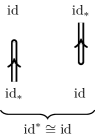
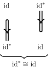
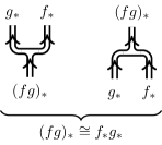
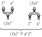
Figure 1: The basic SGNTs as string diagrams

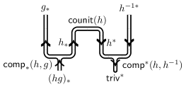
$$h^{-1{*}}\operatorname{\mathsf{counit}}(h)g_{*}\circ h^{-1{*}}h^{*}\operatorname{\mathsf{comp}}_{*}(h,g)\circ\operatorname{\mathsf{comp}}^{*}(h^{-1},h)(hg)_{*}\circ\operatorname{\mathsf{triv}}^{*}(hg)_{*}$$

$$\begin{multlined}(hg)_{*}\xrightarrow{\operatorname{\mathsf{triv}}^{*}}\mathrm{id}^{*}(hg)_{*}=(hh^{-1})^{*}(hg)_{*}\xrightarrow{\operatorname{\mathsf{comp}}^{*}(h,h^{-1})}h^{-1{*}}h^{*}(hg)_{*}\\ \xrightarrow{\operatorname{\mathsf{comp}}_{*}(h,g)}h^{-1{*}}h^{*}h_{*}g_{*}\xrightarrow{\operatorname{\mathsf{counit}}(h)}h^{-1{*}}g_{*}\end{multlined}(hg)_{*}\xrightarrow{\operatorname{\mathsf{triv}}^{*}}\mathrm{id}^{*}(hg)_{*}=(hh^{-1})^{*}(hg)_{*}\xrightarrow{\operatorname{\mathsf{comp}}^{*}(h,h^{-1})}h^{-1{*}}h^{*}(hg)_{*}\\ \xrightarrow{\operatorname{\mathsf{comp}}_{*}(h,g)}h^{-1{*}}h^{*}h_{*}g_{*}\xrightarrow{\operatorname{\mathsf{counit}}(h)}h^{-1{*}}g_{*}$$

Figure 2: Example of a string diagram with corresponding SGNT expressed several ways

An example of the correspondence between string diagrams and SGNTs is given in 2, but we will never be so thorough in labeling them in actual use.

We emphasize that it is important for the correspondence between string diagrams and natural transformations that the string diagram be labeled; i.e. for the edges and components to have the meanings assigned to them by 1. For if not, then the operation of reflecting the string diagram vertically produces another planar graph that is valid combinatorially, but does not necessarily correspond to any SGNT (the corresponding operation on functors $f^{*}g_{*}h^{*}\cdots$ is to swap upper ^∗ and lower _∗, but the resulting basic SGFs are no longer composable). We thank Mitya Boyarchenko for this last observation, however much it forced the restructuring of this paper.

Although the diagram acquires its unique identity as an SGNT only after labeling all the edges, we will almost always omit these labels. We will never assert the identity of an SGNT corresponding to an unlabled diagram without indicating how we would label it, which can (in our applications) always be deduced from the ends by propagating through the various transformations.

String diagram identities.

In this subsection we record all the identities satisfied by string diagrams with two shapes. These can basically be considered the relations in the category whose objects are SGFs and whose morphisms are the string diagrams between two given SGFs. The proofs, which are either direct translation of the corresponding symbolic equations or simple manipulation, are left to the appendix for the convenience of readers who would prefer to get to the point.

Theorem 3.1.

lemfig:adjunctions (Adjunction identities)

Theorem 3.2.

lemfig:compositions (inv) (Composition identities (inverses))

Theorem 3.3.

lemfig:compositions (assoc) (Composition identities (associativity))

Theorem 3.4.

lemfig:trivializations triv (Trivialization identities (trivializations))

Theorem 3.5.

lemfig:trivializations adj (Trivialization identities (adjunctions))

Theorem 3.6.

lemfig:trivializations comp (Trivialization identities (compositions))

Theorem 3.7.

lemfig:adjunction-composition 1 (Adjunction-composition identities (part 1))

Theorem 3.8.

lemfig:adjunction-composition 2 (Adjunction-composition identities (part 2))

Theorem 3.9.

lemfig:compositions (nontrivial) Suppose we have maps of spaces $f$, $g$, $h$, and $k$ and another one $l$ such that $g=lk$ and $h=fl$ (resp. $f=hl$ and $k=lg$). Then we have the first equality (resp. the second equality) below, and similarly for the ^∗ version:

(3.1)

We note that [mccurdy]*Definition 4 establishes a Frobenius algebra as an object in a monoidal category satisfying precisely the above diagrammatic constraints, except that here, the ends of that diagram are not all the same object. This lemma therefore shows that the basic SGFs of a geofibered category form a generalization of a Frobenius algebra, presumably a “Frobenius algebroid” in the same sense as a groupid, though we have not been able to find this term in use.

Theorem 3.10.

lemSD loop We have the equivalence (for either direction of edges and all possible assignments of maps of spaces compatible with the depicted compositions):

(3.2)

4 Uniqueness of reduced forms

We have defined (Definitions LABEL:alternating and LABEL:roof) two reduced forms for an SGF and claimed that they are unique. In this section we prove these claims; the first one is relatively straightforward and does not require string diagrams, but the manipulations of the second one are simplified by their use, so we have placed both of them at this point. Only one general relation needs to be noted here, expressing the “commutation” of unrelated natural transformations.

Theorem 4.1.

lemhorizontal composition verify Let $F=AF_{1}BF_{2}C$ be a composition of functors; let $\phi\colon F_{1}\to G_{1}$ and $\psi\colon F_{2}\to H_{2}$ be natural transformations. Then the following diagram commutes:

$$\includegraphics[valign={M}]{img13}\qquad\qed$$ (4.1)

Uniqueness of the alternating reduction.

Showing that the alternating reduction is unique is a matter of enforcing an inductive structure on its construction, as encapsulated by the following lengthy definition.

Theorem 4.2.

defnstaged morphism Let $\phi\colon F\to G$ be an SGNT; we define a staging structure on it to be the following data:

• A sequence of SGNTs

  $$F=F_{0}\xrightarrow{\gamma_{1}}F_{1}\xrightarrow{\alpha_{2}}F_{2}\cdots\xrightarrow{\alpha_{2n}}F_{2n}=G$$ (4.2)

  together with representations of $\gamma_{i}\in\langle\operatorname{\mathsf{comp}}_{0}\rangle$ and $\alpha_{i}\in\langle\operatorname{\mathsf{triv}}_{0}\rangle$ as products of factors that are basic SGNTs.

• This data must satisfy some conditions. We make reference to the terms of an SGF, its basic SGF composands; a term is trivial if it is of the form $\mathrm{id}_{*}$ or $\mathrm{id}^{*}$; a composable pair is a sequence of two consecutive terms of the form $f_{*}g_{*}$ or $f^{*}g^{*}$. We define the stage of any trivial term or composable pair in any of the intermediate SGFs of the staging structure, together with conditions:

  • The stage of any composable pair of $F_{0}$ is $0$, and of any trivial term is $1$.

  • Let $\alpha$ be any factor of $\alpha_{i}$, acting locally as $t_{1}tt_{2}\to t_{1}t_{2}$, where $t$ is trivial; we require that $t$ have stage $i-1$ and that that both pairs $t_{1}t$ and $tt_{2}$ (when composable) have stage $i$. If $t_{1}t_{2}$ is a composable pair, we define its stage to be $i$. We say that $t$, $t_{1}t_{2}$, and $t_{1}t$ and $tt_{2}$ are affected by $\alpha$.

  • Let $\gamma$ be any factor of $\gamma_{i}$, acting locally as $t_{0}t_{1}t_{2}t_{3}\to t_{0}tt_{3}$, where $t_{1}t_{2}$ is composable. We require that $t_{1}t_{2}$ have stage $i-1$, and that if either of these terms is trivial, then that term has stage $i$. We define the stages of $t_{0}t$ or $tt_{1}$ (when composable), to be those of $t_{0}t_{1}$ and $t_{1}t_{2}$ each; the stage of $t$ (if it is trivial) is $i$, unless $t_{1}$ and $t_{2}$ are both trivial, in which case the stage of $t$ is the larger of their stages. We say that $t$ and $t_{1}t_{2}$ are affected by $\gamma$.

We say that the staging structure is complete at stage $s$ when $s$ is odd if $F_{s}$ has no composable pairs, and when $s$ is even if $F_{s}$ has no trivial terms.

The following fact is trivial:

Theorem 4.3.

lemstage limit In a staged SGNT $\phi\colon F\to G$, any trivial term or composable pair in $F_{s}$ has stage at most $s$, if $s>0$. A term of stage $s$ in $G$ is not affected by any factor of any $\alpha_{i}$ or $\gamma_{i}$ with $i>s$. ∎

In the next few lemmas we establish the strong properties of a complete staging.

Theorem 4.4.

lemcomplete staging If an SGNT with staging $\phi\colon F\to G$ is complete at any stage $s\geq 3$, then it is also complete at stage $s-2$.

Proof 4.5.

Suppose $s$ is odd, and consider a composable pair $t_{1}t_{2}$ in $F_{s-2}$; it has stage $\leq s-2$ by LABEL:stage_limit. It is thus not possible for either term to be affected by a factor of $\alpha_{s-1}$, so this pair persists into $F_{s-1}$. There, since $t_{1}t_{2}$ still has stage $\leq s-2$, it cannot be acted on by a factor of $\gamma_{s}$ so this space in $F_{s-1}$ will remain in a composable pair in $F_{s}$.

Suppose $s$ is even, and consider a trivial term $t$ in $F_{s-2}$. By LABEL:stage_limit it has stage $\leq s-2$, so it is not affected by any factor of $\gamma_{s-1}$, so it persists into $F_{s-1}$. There, it has the same stage and so cannot be affected by any factor of $\alpha_{s}$, so it persists into $F_{s}$, forming a trivial term there.

Theorem 4.6.

corcomplete staging induct If $\phi\colon F\to G$ has a staging such that $G$ has neither composable pairs nor trivial terms, then it is complete at every stage $s\geq 1$.

Proof 4.7.

It is vacuously compatible with the definition of a staging to define $F_{2n+2}=F_{2n+1}=F_{2n}=G$ with $\alpha_{2n+2}=\gamma_{2n+1}=\mathrm{id}$, with which convention $\phi$ is complete at stages $2n+1$ and $2n$, so by induction on LABEL:complete_staging, at every stage $s\geq 1$.

Theorem 4.8.

lemcomplete staging determined If $\phi\colon F\to G$ has a staging that is complete at every stage $s\geq 1$, then all the intermediate SGFs $F_{i}$ and SGNTs $\alpha_{i}$ and $\beta_{i}$ are uniquely determined by $F$.

Proof 4.9.

It is clear that if $\phi$ is complete at $F_{1}$, then $F_{1}$ must be obtained by composing all composable pairs of $F_{0}$; this is well-defined regardless of order by 1.4 and gives $\gamma_{1}$ uniquely. Then it is also clear that if $\phi$ is complete at $F_{2}$, it must be obtained by deleting all trivial terms of $F_{1}$, which is well-defined regardless of order by LABEL:horizontal_composition_verify and gives $\alpha_{2}$ uniquely. By induction, the lemma follows.

Now we turn to the construction of a staging on a given SGNT.

Theorem 4.10.

lemstage associativity Let $\phi\colon F\to G$ have a staging; then any reordering of the factors of any $\gamma_{i}$ by associativity, as in 1.4, is a valid staging.

Proof 4.11.

Given two overlapping compositions:

$$t_{0}((t_{1}t_{2})t_{3})t_{4} t_{0}(t_{1}(t_{2}t_{3}))t_{4}$$ (4.3)

suppose that the first grouping satisfies the conditions of a staging. Thus, $t_{1}t_{2}$ has stage $\geq i-1$ and each trivial $t_{j}$ has stage $i$. Let $t$ be their composition, so in particular, $tt_{3}$ has the same stage as $t_{2}t_{3}$ and, as it is acted on by another factor of $\gamma_{i}$, thus has stage $\geq i-1$. It follows that $t_{2}t_{3}$ has stage $\geq i-1$, and likewise that if $t_{3}$ is trivial, then it has stage $i$. Therefore the second grouping also satisfies the conditions of a staging. Furthermore, the product of the first group has stage $i$ unless all three of $t_{1}$, $t_{2}$, and $t_{3}$ are trivial, which is the same exception as for the second group, in which case its stage is the maximum of their stages. So the results of each grouping are identical.

Theorem 4.12.

lemstage comp Let $\phi\colon F\to G$ have a staging and let $t_{0}t_{1}t_{2}t_{3}t_{4}t_{5}$ be a sequence of composable terms in $G$. Suppose that the staging can be extended by composing $t_{2}t_{3}$ or by composing both $t_{1}t_{2}$ and $t_{3}t_{4}$. Then it can be extended by the sequence of compositions

$$t_{0}(t_{1}((t_{2}t_{3})t_{4}))t_{5}.$$ (4.4)

Proof 4.13.

We suppose that we are constructing stage $2n+1$ of $\phi$. By the first assumption, the stage of $t_{2}t_{3}$ is $2n$. By construction, $t=(t_{2}t_{3})$, if trivial, has stage $2n+1$ and both pairs $t_{1}t$ and $tt_{4}$ have the same stages as, respectively, $t_{1}t_{2}$ and $t_{3}t_{4}$. By the second assumption, the latter stages are $2n$ and each $t_{1,4}$ (when trivial) has stage $2n+1$. Therefore, the pair $tt_{4}$ may be composed in a staging, with value $u$ (if trivial) of stage $2n+1$ and the pair $t_{1}u$ having stage that of $t_{1}t$, which is the same as that of $t_{1}t_{2}$, which is $2n$. So the pair $t_{1}u$ may be composed as well.

Theorem 4.14.

corstage extend comp Let $\phi\colon F\to G$ have a staging ending at stage $2n+1$, and let $\psi\in\operatorname{\mathsf{comp}}_{0}$ have domain $G$ affecting a pair $t_{1}t_{2}$ of stage $\leq 2n-2$. Define a factorization of $\gamma_{2n+1}$, using LABEL:stage_limit and associativity 1.4, as $\gamma^{1}\gamma^{0}$, where $\gamma^{0}$ does not affect $t_{1}t_{2}$ and $\gamma^{1}$ is a pair of two $\operatorname{\mathsf{comp}}_{0}$ factors having values $t_{1}$ and $t_{2}$ respectively. Let $\phi^{\prime}$ be the portion of $\phi$ up to stage $2n$ and let $\psi^{\prime}$ be $\psi$ applied to the codomain of $\gamma^{0}$. Then, if $\psi^{\prime}\gamma^{0}\phi^{\prime}$ has a staging, so does $\psi\phi$.

Proof 4.15.

By LABEL:stage_associativity, the SGNT $\gamma^{1}\gamma^{0}\phi^{\prime}$ has a staging, so by definition, so does $\gamma^{0}\phi^{\prime}$, and then LABEL:stage_comp applies.

Theorem 4.16.

lemstaging induct Let $\phi\colon F\to G$ have a staging, and let $\psi$ be a basic SGNT either in $\operatorname{\mathsf{comp}}_{0}$ or $\operatorname{\mathsf{triv}}_{0}$ composable with $\phi$. Then $\psi\phi$ has a staging.

Proof 4.17.

The proof is by descending induction, with the two terminal cases:

1. $\psi\in\operatorname{\mathsf{triv}}_{0}$ acts as $t_{1}tt_{2}\to t_{1}t_{2}$, where the triple satisfies the conditions of a staging at stage $2n$;

2. $\psi\in\operatorname{\mathsf{comp}}_{0}$ acts as $t_{1}t_{2}\to t$, where the composable pair satisfies the conditions of a staging at stage $2n+1$;

In the first, we can append $\psi$ to $\alpha_{2n}$, satisfying the definition of a staging. In the second, we can begin $\gamma_{2n+1}$ with $\psi$, satisfying the definition of a staging. Note that these each apply, respectively, at stages $2$ and $1$, so the induction is well-founded.

Suppose that $\psi\in\operatorname{\mathsf{triv}}_{0}$ acts on a trivial term $t$; if 1 does not apply, then either $t$ has stage $<2n-1$ or one of the pairs including $t$ is composable; if the conditions for a composition in a staging do not apply to it, then either the pair has stage $<2n$ or the other term is trivial of stage $<2n-1$.

Suppose that $\psi\in\operatorname{\mathsf{comp}}_{0}$ acts on a composable pair $t_{1}t_{2}$; if 2 does not apply, then either its stage is $<2n$, or one of the terms $t_{i}$ is trivial of stage $<s$.

In either case, we have identified a pair $t_{1}t_{2}$ such that either at least one term is trivial and has stage $<2n-1$, or $t_{1}t_{2}$ itself has stage $<2n$; when $\psi\in\operatorname{\mathsf{triv}}_{0}$ it acts on one of the $t_{i}$, and when $\psi\in\operatorname{\mathsf{comp}}_{0}$ it acts on $t_{1}t_{2}$. Then by 1.6, we can replace $\psi$ with either the composition of $t_{1}t_{2}$ or a trivialization of either trivial $t_{i}$. In the latter case, by LABEL:horizontal_composition_verify, we may “commute” $\psi$ with all $\beta_{i}$ and $\gamma_{i}$ down to $F_{s}$. In the former case, we do this with $\psi\in\operatorname{\mathsf{comp}}_{0}$ using LABEL:stage_extend_comp and LABEL:horizontal_composition_verify. Either way, the proof follows by induction.

Theorem 4.18.

propalternating unique For any SGF $F$, there exists a unique map $F\to G$ in $\langle\operatorname{\mathsf{comp}}_{0}\cup\operatorname{\mathsf{triv}}_{0}\rangle$ with $G$ alternating.

Proof 4.19.

Any such SGNT has a staging by induction on LABEL:staging_induct, and $G$ has neither trivial terms nor composable pairs by definition of an alternating SGF. Therefore, by LABEL:complete_staging_induct, it is complete at every stage, so by LABEL:complete_staging_determined it is uniquely determined by $F$. Given $F$ alone, such a map exists by the construction in the proof of that lemma.

Theorem 4.20.

corbig alternating unique If $\phi\colon F\to G$ is in $\langle\operatorname{\mathsf{comp}}\cup\operatorname{\mathsf{triv}}\rangle$, then it is unique there, and $F$ and $G$ have the same alternating reduction.

Proof 4.21.

Write $\phi$ as an alternating composition of $\langle\operatorname{\mathsf{comp}}_{0}\cup\operatorname{\mathsf{triv}}_{0}\rangle$ and its inverses. By LABEL:alternating_unique, either one preserves both the alternating reduction and the map to it, so this is true of $\phi$ as a whole by induction. If there is another such map $\phi^{\prime}$, then $\phi^{-1}\phi^{\prime}$ is a self-map of $F$ preserving the map to its alternating reduction. Since that map is an isomorphism, we have $\phi^{-1}\phi^{\prime}=\mathrm{id}$.

Relations.

To deal with the roof and its additional complications arising from the base change morphisms, we prove a number of “commutation relations” among $\operatorname{\mathsf{comp}}_{0}$, $\operatorname{\mathsf{triv}}_{0}$, and $\operatorname{\mathsf{bc}}$, beginning with rewriting some especially trivial transformations in terms of simpler ones. In this subsection, we use $\operatorname{\mathsf{cd}}$ instead of $\operatorname{\mathsf{bc}}$ to emphasize the fundamentally diagrammatic nature of the arguments; following that, we will be forced for practical reasons to specialize.

Theorem 4.22.

lemCD trivial isomorphisms We have identities

$$\operatorname{\mathsf{cd}}(f,\mathrm{id};f,\mathrm{id}) = \operatorname{\mathsf{triv}}_{*}^{-1}f^{*} \circ f^{*}\operatorname{\mathsf{triv}}_{*} \colon f^{*}\mathrm{id}_{*} \to\mathrm{id}_{*}f^{*}$$ (4.5a)

$$\operatorname{\mathsf{cd}}(\mathrm{id},f;\mathrm{id},f) = f_{*}\operatorname{\mathsf{triv}}^{{*}{-1}} \circ\operatorname{\mathsf{triv}}^{*}f_{*} \colon\mathrm{id}^{*}f_{*} \to f_{*}\mathrm{id}^{*}.$$ (4.5b)

Proof 4.23.

First, we note that according to the definition 1.12, we have as a string diagram

$$\operatorname{\mathsf{cd}}(f,g;\tilde{f},\tilde{g})=\includegraphics[valign={M}]{img14}$$ (4.6)

Now, for the claimed identities, moving the right-hand side terms to the left, they are equivalent to the two string diagram identities

(4.7)

the first of which follows from LABEL:fig:trivializations_adj and then LABEL:fig:trivializations_comp (twice each), and the second of which follows from LABEL:fig:trivializations_comp (twice) and then LABEL:fig:adjunctions.

For those nontrivial SGNTs that do “interact”, we have the following relations:

Theorem 4.24.

lemcommutation relations The following “commutation relations” hold in $\operatorname{\mathsf{SGNT}}_{0}$:

1. We have, for any composable maps $f$ and $g$ of spaces:

   $$\begin{multlined}\bigl{(}f_{*}\mathrm{id}_{*}g_{*}\xrightarrow{\operatorname{\mathsf{triv}}_{*}}f_{*}g_{*}\xrightarrow{\operatorname{\mathsf{comp}}_{*}(g,f)}(fg)_{*}\bigr{)}\\ =\bigl{(}f_{*}\mathrm{id}_{*}g_{*}\xrightarrow{\operatorname{\mathsf{comp}}_{*}(g,\mathrm{id})}f_{*}g_{*}\xrightarrow{\operatorname{\mathsf{comp}}_{*}(g,f)}(fg)_{*}\bigr{)}\end{multlined}\bigl{(}f_{*}\mathrm{id}_{*}g_{*}\xrightarrow{\operatorname{\mathsf{triv}}_{*}}f_{*}g_{*}\xrightarrow{\operatorname{\mathsf{comp}}_{*}(g,f)}(fg)_{*}\bigr{)}\\ =\bigl{(}f_{*}\mathrm{id}_{*}g_{*}\xrightarrow{\operatorname{\mathsf{comp}}_{*}(g,\mathrm{id})}f_{*}g_{*}\xrightarrow{\operatorname{\mathsf{comp}}_{*}(g,f)}(fg)_{*}\bigr{)}$$ (4.8c)

   $$\begin{multlined}\bigl{(}f_{*}\mathrm{id}^{*}g_{*}\xrightarrow{\operatorname{\mathsf{triv}}^{*}}f_{*}g_{*}\xrightarrow{\operatorname{\mathsf{comp}}_{*}(g,f)}(fg)_{*}\bigr{)}\\ =\bigl{(}f_{*}\mathrm{id}^{*}g_{*}\xrightarrow{\operatorname{\mathsf{cd}}(g,\mathrm{id};g,\mathrm{id})}f_{*}g_{*}\mathrm{id}^{*}\xrightarrow{\operatorname{\mathsf{comp}}_{*}(g,f)}(fg)_{*}\mathrm{id}^{*}\xrightarrow{\operatorname{\mathsf{triv}}^{*}}(fg)_{*}\bigr{)}\end{multlined}\bigl{(}f_{*}\mathrm{id}^{*}g_{*}\xrightarrow{\operatorname{\mathsf{triv}}^{*}}f_{*}g_{*}\xrightarrow{\operatorname{\mathsf{comp}}_{*}(g,f)}(fg)_{*}\bigr{)}\\ =\bigl{(}f_{*}\mathrm{id}^{*}g_{*}\xrightarrow{\operatorname{\mathsf{cd}}(g,\mathrm{id};g,\mathrm{id})}f_{*}g_{*}\mathrm{id}^{*}\xrightarrow{\operatorname{\mathsf{comp}}_{*}(g,f)}(fg)_{*}\mathrm{id}^{*}\xrightarrow{\operatorname{\mathsf{triv}}^{*}}(fg)_{*}\bigr{)}$$ (4.8f)

   $$\begin{multlined}\bigl{(}f^{*}\mathrm{id}^{*}g^{*}\xrightarrow{\operatorname{\mathsf{triv}}^{*}}f^{*}g^{*}\xrightarrow{\operatorname{\mathsf{comp}}^{*}(f,g)}(gf)^{*}\bigr{)}\\ =\bigl{(}f^{*}\mathrm{id}^{*}g^{*}\xrightarrow{\operatorname{\mathsf{comp}}^{*}(\mathrm{id},g)}f^{*}g^{*}\xrightarrow{\operatorname{\mathsf{comp}}^{*}(f,g)}(gf)^{*}\bigr{)}\end{multlined}\bigl{(}f^{*}\mathrm{id}^{*}g^{*}\xrightarrow{\operatorname{\mathsf{triv}}^{*}}f^{*}g^{*}\xrightarrow{\operatorname{\mathsf{comp}}^{*}(f,g)}(gf)^{*}\bigr{)}\\ =\bigl{(}f^{*}\mathrm{id}^{*}g^{*}\xrightarrow{\operatorname{\mathsf{comp}}^{*}(\mathrm{id},g)}f^{*}g^{*}\xrightarrow{\operatorname{\mathsf{comp}}^{*}(f,g)}(gf)^{*}\bigr{)}$$ (4.8i)

   $$\begin{multlined}\bigl{(}f^{*}\mathrm{id}_{*}g^{*}\xrightarrow{\operatorname{\mathsf{triv}}_{*}}f^{*}g^{*}\xrightarrow{\operatorname{\mathsf{comp}}^{*}(f,g)}(gf)^{*}\bigr{)}\\ =\bigl{(}f^{*}\mathrm{id}_{*}g^{*}\xrightarrow{\operatorname{\mathsf{cd}}(\mathrm{id},f;\mathrm{id},f)}\mathrm{id}_{*}f^{*}g^{*}\xrightarrow{\operatorname{\mathsf{comp}}^{*}(f,g)}\mathrm{id}^{*}(gf)^{*}\xrightarrow{\operatorname{\mathsf{triv}}^{*}}(gf)^{*}\bigr{)}\end{multlined}\bigl{(}f^{*}\mathrm{id}_{*}g^{*}\xrightarrow{\operatorname{\mathsf{triv}}_{*}}f^{*}g^{*}\xrightarrow{\operatorname{\mathsf{comp}}^{*}(f,g)}(gf)^{*}\bigr{)}\\ =\bigl{(}f^{*}\mathrm{id}_{*}g^{*}\xrightarrow{\operatorname{\mathsf{cd}}(\mathrm{id},f;\mathrm{id},f)}\mathrm{id}_{*}f^{*}g^{*}\xrightarrow{\operatorname{\mathsf{comp}}^{*}(f,g)}\mathrm{id}^{*}(gf)^{*}\xrightarrow{\operatorname{\mathsf{triv}}^{*}}(gf)^{*}\bigr{)}$$ (4.8l)

2. We have, referring to 1.10:

   $$\begin{multlined}\bigl{(}g^{*}\mathrm{id}_{*}f_{*}\xrightarrow{\operatorname{\mathsf{triv}}_{*}}g^{*}f_{*}\xrightarrow{\operatorname{\mathsf{cd}}(f,g;\tilde{f},\tilde{g})}\tilde{f}_{*}\tilde{g}^{*}\bigr{)}\\ =\bigl{(}g^{*}\mathrm{id}_{*}f_{*}\xrightarrow{\operatorname{\mathsf{comp}}_{*}(f,\mathrm{id})}g^{*}f_{*}\xrightarrow{\operatorname{\mathsf{cd}}(f,g;\tilde{f},\tilde{g})}\tilde{f}_{*}\tilde{g}^{*}\bigr{)}\end{multlined}\bigl{(}g^{*}\mathrm{id}_{*}f_{*}\xrightarrow{\operatorname{\mathsf{triv}}_{*}}g^{*}f_{*}\xrightarrow{\operatorname{\mathsf{cd}}(f,g;\tilde{f},\tilde{g})}\tilde{f}_{*}\tilde{g}^{*}\bigr{)}\\ =\bigl{(}g^{*}\mathrm{id}_{*}f_{*}\xrightarrow{\operatorname{\mathsf{comp}}_{*}(f,\mathrm{id})}g^{*}f_{*}\xrightarrow{\operatorname{\mathsf{cd}}(f,g;\tilde{f},\tilde{g})}\tilde{f}_{*}\tilde{g}^{*}\bigr{)}$$ (4.9c)

   $$\begin{multlined}\bigl{(}g^{*}\mathrm{id}^{*}f_{*}\xrightarrow{\operatorname{\mathsf{triv}}^{*}}g^{*}f_{*}\xrightarrow{\operatorname{\mathsf{cd}}(f,g;\tilde{f},\tilde{g})}\tilde{f}_{*}\tilde{g}^{*}\bigr{)}\\ =\bigl{(}g^{*}\mathrm{id}^{*}f_{*}\xrightarrow{\operatorname{\mathsf{comp}}^{*}(g,\mathrm{id})}g^{*}f_{*}\xrightarrow{\operatorname{\mathsf{cd}}(f,g,\tilde{f},\tilde{g})}\tilde{f}_{*}\tilde{g}^{*}\bigr{)}\end{multlined}\bigl{(}g^{*}\mathrm{id}^{*}f_{*}\xrightarrow{\operatorname{\mathsf{triv}}^{*}}g^{*}f_{*}\xrightarrow{\operatorname{\mathsf{cd}}(f,g;\tilde{f},\tilde{g})}\tilde{f}_{*}\tilde{g}^{*}\bigr{)}\\ =\bigl{(}g^{*}\mathrm{id}^{*}f_{*}\xrightarrow{\operatorname{\mathsf{comp}}^{*}(g,\mathrm{id})}g^{*}f_{*}\xrightarrow{\operatorname{\mathsf{cd}}(f,g,\tilde{f},\tilde{g})}\tilde{f}_{*}\tilde{g}^{*}\bigr{)}$$ (4.9f)

3. Consider the large commutative diagram

   (4.10)

   We have:

   $$\begin{multlined}\bigl{(}g^{*}f_{*}h_{*}\xrightarrow{\operatorname{\mathsf{comp}}_{*}(h,f)}g^{*}(fh)_{*}\xrightarrow{\operatorname{\mathsf{cd}}(fh,g;\tilde{f}\tilde{h},k)}(\tilde{f}\tilde{h})_{*}k^{*}\bigr{)}\\ =\bigl{(}g^{*}f_{*}h_{*}\xrightarrow{\operatorname{\mathsf{cd}}(f,g;\tilde{f},\tilde{g})}\tilde{f}_{*}\tilde{g}^{*}h_{*}\xrightarrow{\operatorname{\mathsf{cd}}(h,\tilde{g};\tilde{h},k)}\tilde{f}_{*}\tilde{h}_{*}k^{*}\xrightarrow{\operatorname{\mathsf{comp}}_{*}(\tilde{h},\tilde{f})}(\tilde{f}\tilde{h})_{*}k^{*}\bigr{)}\end{multlined}\bigl{(}g^{*}f_{*}h_{*}\xrightarrow{\operatorname{\mathsf{comp}}_{*}(h,f)}g^{*}(fh)_{*}\xrightarrow{\operatorname{\mathsf{cd}}(fh,g;\tilde{f}\tilde{h},k)}(\tilde{f}\tilde{h})_{*}k^{*}\bigr{)}\\ =\bigl{(}g^{*}f_{*}h_{*}\xrightarrow{\operatorname{\mathsf{cd}}(f,g;\tilde{f},\tilde{g})}\tilde{f}_{*}\tilde{g}^{*}h_{*}\xrightarrow{\operatorname{\mathsf{cd}}(h,\tilde{g};\tilde{h},k)}\tilde{f}_{*}\tilde{h}_{*}k^{*}\xrightarrow{\operatorname{\mathsf{comp}}_{*}(\tilde{h},\tilde{f})}(\tilde{f}\tilde{h})_{*}k^{*}\bigr{)}$$ (4.11c)

   $$\begin{multlined}\bigl{(}h^{*}f^{*}g_{*}\xrightarrow{\operatorname{\mathsf{comp}}^{*}(h,f)}(fh)^{*}g_{*}\xrightarrow{\operatorname{\mathsf{cd}}(g,fh;k,\tilde{f}\tilde{h})}k_{*}(\tilde{f}\tilde{h})^{*}\bigr{)}\\ =\bigl{(}h^{*}f^{*}g_{*}\xrightarrow{\operatorname{\mathsf{cd}}(g,f;\tilde{g},\tilde{f})}h^{*}\tilde{g}_{*}\tilde{f}^{*}\xrightarrow{\operatorname{\mathsf{cd}}(\tilde{g},h;k,\tilde{h})}k_{*}\tilde{h}^{*}\tilde{f}^{*}\xrightarrow{\operatorname{\mathsf{comp}}^{*}(\tilde{h},\tilde{f})}k_{*}(\tilde{f}\tilde{h})^{*}\bigr{)}\end{multlined}\bigl{(}h^{*}f^{*}g_{*}\xrightarrow{\operatorname{\mathsf{comp}}^{*}(h,f)}(fh)^{*}g_{*}\xrightarrow{\operatorname{\mathsf{cd}}(g,fh;k,\tilde{f}\tilde{h})}k_{*}(\tilde{f}\tilde{h})^{*}\bigr{)}\\ =\bigl{(}h^{*}f^{*}g_{*}\xrightarrow{\operatorname{\mathsf{cd}}(g,f;\tilde{g},\tilde{f})}h^{*}\tilde{g}_{*}\tilde{f}^{*}\xrightarrow{\operatorname{\mathsf{cd}}(\tilde{g},h;k,\tilde{h})}k_{*}\tilde{h}^{*}\tilde{f}^{*}\xrightarrow{\operatorname{\mathsf{comp}}^{*}(\tilde{h},\tilde{f})}k_{*}(\tilde{f}\tilde{h})^{*}\bigr{)}$$ (4.11f)

Proof 4.25.

For 4.8c and 4.8i, we can directly apply 1.6 for the former (and its analogue LABEL:fig:trivializations_comp for the latter), ignoring the second composand. The same goes for both equations 4.9. The remainder we prove using string diagrams.

For 4.8f, the string diagrams of the left and right transformations are, respectively:

(4.12)

Clearly it is the latter diagram that needs to be simplified; to understand it, the blue sub-diagram is $\operatorname{\mathsf{cd}}(g,\mathrm{id};\allowbreak g,\mathrm{id})$, the red one is $\operatorname{\mathsf{comp}}_{*}(g,f)$, and the black one is $\operatorname{\mathsf{triv}}^{*}$. We recall our convention on omitting labels from diagrams; there should be no ambiguity provided that one recalls the labels of the ends.

We begin by applying LABEL:fig:trivializations_comp to the one $\operatorname{\mathsf{triv}}$, simplifying it to the first diagram below, which then transforms using LABEL:fig:adjunction-composition_2 on the blue subdiagram:

(4.13)

Finally, we break the identity (middle lower) string according to LABEL:fig:trivializations_triv and remove the associated $\operatorname{\mathsf{unit}}$-$\operatorname{\mathsf{triv}}$ combination using LABEL:fig:trivializations_adj and then LABEL:fig:trivializations_comp again, leaving the first figure of 4.12, as desired. The same computation applies to 4.8l (or, to avoid repeating the same work: take the above computation, reverse all the arrows, and reflect it horizontally).

For 4.11c, we again render the two transformations as diagrams, which are somewhat more complex:

(4.14)

To parse the first diagram, the blue sub-diagram is $\operatorname{\mathsf{comp}}_{*}(h,f)$ and the red one is $\operatorname{\mathsf{cd}}(fh,g;\allowbreak\tilde{f}\tilde{h},k)$. To parse the second diagram, the blue sub-diagram is $\operatorname{\mathsf{cd}}(f,g;\allowbreak\tilde{f},\tilde{g})$, the red one is $\operatorname{\mathsf{cd}}(h,\tilde{g};\allowbreak\tilde{h},k)$, and the black one is $\operatorname{\mathsf{comp}}_{*}(\tilde{h},\tilde{f})$. Simplifying this requires a number of steps but as a first major goal we eliminate the loop. As usual, we use matching colors to indicate changes in the diagrams, where violet denotes a subdiagram that is both blue and red (i.e. is changed both from and to the adjacent diagrams).

(4.15)

In the first equality we use LABEL:fig:adjunction-composition_1, and in the second, we use LABEL:SD_loop. Now we paste this into the rest of 4.14:

(4.16)

where the first equality is LABEL:fig:compositions_(assoc) again and the second is LABEL:fig:adjunction-composition_1. The last diagram is the left diagram of 4.14, as desired. The proof of 4.11f is the same (that is, with arrows reversed and the diagrams reflected horizontally).

Uniqueness of the roof.

Now we pursue a “normal form” for the roof similar to the “staging” defined for the alternating reduction. It is much less complicated, however.

Theorem 4.26.

lemSGNT CD ordering We have $\langle\operatorname{\mathsf{comp}}_{0}\cup\operatorname{\mathsf{triv}}_{0}\cup\operatorname{\mathsf{bc}}\rangle=\langle\operatorname{\mathsf{triv}}_{0}\rangle\langle\operatorname{\mathsf{comp}}_{0}\rangle\langle\operatorname{\mathsf{bc}}\rangle$.

Proof 4.27.

Before proceeding, note that using LABEL:commutation_relationsb from “left to right” requires making a choice of the individual morphisms $\tilde{f}$, $\tilde{g}$, and $\tilde{h}$ given only the composition $\tilde{h}\tilde{f}$; this may not, in general, be possible, but is in fact canonical if we assume the outer rectangle is cartesian (then we may take $\tilde{g}$ to be the base change of $g$). This is why we specialize to $\operatorname{\mathsf{bc}}$ in this corollary, aside from the applications.

Now, it follows from LABEL:horizontal_composition_verify and the cases a and b of LABEL:commutation_relations that $\langle\operatorname{\mathsf{comp}}_{0}\cup\operatorname{\mathsf{triv}}_{0}\cup\operatorname{\mathsf{cd}}\rangle=\langle\operatorname{\mathsf{triv}}_{0}\rangle\langle\operatorname{\mathsf{comp}}_{0}\cup\operatorname{\mathsf{cd}}\rangle$, and it follows from case c that we have $\langle\operatorname{\mathsf{comp}}_{0}\cup\operatorname{\mathsf{cd}}\rangle=\langle\operatorname{\mathsf{comp}}_{0}\rangle\langle\operatorname{\mathsf{cd}}\rangle$.

Although this proves that any $\phi\in\langle\operatorname{\mathsf{comp}}_{0}\cup\operatorname{\mathsf{triv}}_{0}\cup\operatorname{\mathsf{bc}}\rangle$ can be written as $\alpha\beta\gamma$ with $\alpha\in\langle\operatorname{\mathsf{triv}}_{0}\rangle$, $\beta\in\langle\operatorname{\mathsf{comp}}_{0}\rangle$, and $\gamma\in\langle\operatorname{\mathsf{bc}}\rangle$, the intermediate functors $\operatorname{dom}\alpha=\operatorname{cod}\beta$ and $\operatorname{dom}\beta=\operatorname{cod}\gamma$ are not canonical. In the general case this is unfixable, though the next lemma remains valid. In the case of the roof, this is fortunately all that is required.

Theorem 4.28.

lemcanonical triv Let $F$ be any SGF and let $\phi\colon G\to F$ be in $\langle\operatorname{\mathsf{bc}}\cup\operatorname{\mathsf{comp}}_{0}\cup\operatorname{\mathsf{triv}}_{0}\rangle$. Then there exists an SGF $F_{\operatorname{\mathsf{triv}}}=F_{l}FF_{r}$ and an SGNT $\phi_{\operatorname{\mathsf{triv}}}=\phi_{l}F\phi_{r}\colon F_{\operatorname{\mathsf{triv}}}\to F$, having the properties that:

• $F_{l}=\mathrm{id}$ if and only if $\phi_{l}=\mathrm{id}$; otherwise, $F_{l}=\mathrm{id}_{*}$ and $\phi_{l}=\operatorname{\mathsf{triv}}_{*}$, and unless $F=f^{*}F_{1}$ starts with a ^∗, we have $F_{l}=\mathrm{id}$,

• $F_{r}=\mathrm{id}$ if and only if $\phi_{r}=\mathrm{id}$; otherwise, $F_{r}=\mathrm{id}^{*}$ and $\phi_{r}=\operatorname{\mathsf{triv}}^{*}$, and unless $F=F_{1}f_{*}$ ends with a _∗, we have $F_{r}=\mathrm{id}$,

and a $\psi\colon G\to F_{\operatorname{\mathsf{triv}}}$ in $\langle\operatorname{\mathsf{bc}}\cup\operatorname{\mathsf{comp}}_{0}\rangle$ such that $\phi=\phi_{\operatorname{\mathsf{triv}}}\psi$.

Proof 4.29.

By LABEL:SGNT_CD_ordering, it suffices to assume $\phi\in\langle\operatorname{\mathsf{triv}}_{0}\rangle$. By 4.5a, any $\operatorname{\mathsf{triv}}_{*}$ in the configuration $f^{*}\operatorname{\mathsf{triv}}_{*}\colon f^{*}\mathrm{id}_{*}\to f^{*}$ can be replaced by $\operatorname{\mathsf{bc}}(f,\mathrm{id})$ followed by $\operatorname{\mathsf{triv}}_{*}f^{*}\colon\mathrm{id}_{*}f^{*}\to f^{*}$. Inductively, then, any configuration $f_{1}^{*}\cdots f_{n}^{*}\operatorname{\mathsf{triv}}_{*}$ is equal to $\operatorname{\mathsf{triv}}_{*}f_{1}^{*}\cdots f_{n}^{*}$ following a sequence of base change morphisms. Similarly, by 4.5b we may convert $\operatorname{\mathsf{triv}}^{*}f_{1{*}}\cdots f_{n{*}}$ to $f_{1{*}}\cdots f_{n{*}}\operatorname{\mathsf{triv}}^{*}$ following a sequence of base changes.

Analogously, by 1.6, any $\operatorname{\mathsf{triv}}_{*}$ in the configuration $\operatorname{\mathsf{triv}}_{*}f_{*}$ or $f_{*}\operatorname{\mathsf{triv}}_{*}$ can be replaced wholesale with simply $\operatorname{\mathsf{comp}}_{*}(f,\mathrm{id})$ or $\operatorname{\mathsf{comp}}_{*}(\mathrm{id},f)$ respectively. Likewise for $\operatorname{\mathsf{triv}}^{*}$.

Now, by LABEL:horizontal_composition_verify, all $\operatorname{\mathsf{triv}}_{*}$ and $\operatorname{\mathsf{triv}}^{*}$ morphisms “commute”, so we may assume that those covered in the first paragraph occur first on the composition of $\phi$, followed by those covered in the second paragraph. It follows that the only trivializations that cannot be eliminated by this combination are those appearing in the configuration $\operatorname{\mathsf{triv}}_{*}f^{*}$ at the left end, or $f_{*}\operatorname{\mathsf{triv}}^{*}$ at the right end of the composition, giving $F_{\operatorname{\mathsf{triv}}}$ and $\phi_{\operatorname{\mathsf{triv}}}$, and the above construction furnishes $\psi$.

Now we can prove LABEL:roof_morphism.

Theorem 4.30.

proproof morphism uniqueness For any SGF $F$, its roof $\operatorname{roof}(F)$ is the unique SGF of the form $a_{*}b^{*}$ admitting admitting a map $\operatorname{roof}(F)\colon F\to a_{*}b^{*}$ in $\operatorname{\mathsf{SGNT}}_{0}^{+}$, and this map is unique.

Proof 4.31.

Let $\phi\colon F\to\operatorname{roof}(F)$ be in $\operatorname{\mathsf{SGNT}}_{0}^{+}$; that is, in $\langle\operatorname{\mathsf{bc}}\cup\operatorname{\mathsf{comp}}_{0}\cup\operatorname{\mathsf{triv}}_{0}\rangle$. LABEL:SGNT_CD_ordering then places it in the form $\alpha\gamma\beta$ with $\alpha\in\langle\operatorname{\mathsf{triv}}_{0}\rangle$, $\gamma\in\langle\operatorname{\mathsf{comp}}_{0}\rangle$, and $\beta\in\langle\operatorname{\mathsf{bc}}\rangle$, and furthermore by LABEL:canonical_triv, $\alpha=\mathrm{id}$, since $\operatorname{roof}(F)=a_{F{*}}b_{F}^{*}$.

Write $\beta\colon F\to G$; since $\gamma\colon G\to a_{G{*}}b_{G}^{*}$ is in $\operatorname{\mathsf{comp}}_{0}$, we must have $G$ of the form $(a_{1{*}}\cdots a_{i{*}})(b_{j}^{*}\cdots b_{1}^{*})$ and $\beta\in\langle\operatorname{\mathsf{bc}}\rangle$; thus, the maps $a_{k}$ and $b_{k}$ furnish the projections of the final object mapping to the diagram of $F$ described in LABEL:roof, and in particular, $G$ is unique. We will write $G=F_{\operatorname{\mathsf{bc}}}$.

The proof then reduces to two claims: that the map $\gamma\colon F_{\operatorname{\mathsf{bc}}}\to\operatorname{roof}(F)$ is unique in $\langle\operatorname{\mathsf{comp}}_{0}\rangle$, and that the map $\beta\colon F\to F_{\operatorname{\mathsf{bc}}}$ is unique in $\langle\operatorname{\mathsf{bc}}\rangle$. The former is simple: since $\operatorname{roof}(F)=a_{F{*}}b_{F}^{*}$, the map $\gamma$ must be of the form $(\operatorname{\mathsf{comp}}_{*}(?,?)\cdots)(\operatorname{\mathsf{comp}}^{*}(?,?)\cdots)$; i.e. the _∗ and ^∗ compositions do not interact. Then by 1.4, both factors are fully associative, so $\gamma$ is unique.

For the latter, the proof follows directly from LABEL:horizontal_composition_verify but only with the right words. By definition, $\beta\in\langle\operatorname{\mathsf{bc}}\rangle$ is a composition of base change morphisms, which we may view as rewriting the string of basic SGFs $F$: each $\operatorname{\mathsf{bc}}(f,g)$ replaces $g^{*}f_{*}$ with $\tilde{f}_{*}\tilde{g}^{*}$; we will call the two-letter space it affects its support. We will say that given any particular representation of $\beta$ as a composition, the basic SGFs of $F$ itself have level $1$ and that each replacement increases the level of each basic SGF by $1$. We will say that the level of a specific $\operatorname{\mathsf{bc}}(f,g)$ factor is $n$ if that is the larger of the levels of $f$ and $g$.

By definition of level, if a factor of level $1$ follows any other factor, then their supports must be disjoint, and therefore, they are subject to LABEL:horizontal_composition_verify. Therefore, $\beta$ may be written with all the factors of level $1$ coming first; i.e. $\beta=\beta\beta_{0}$, where $\beta_{0}$ is a composition of level-$1$ factors and $\beta$, a composition of higher-level factors.

The set of possible level-$1$ factors is the set of possible base change morphisms out of $F$, each of which correspond to a configuration $g^{*}f_{*}$ in $F$. Since in $\operatorname{roof}(F)$, no such configurations remain, each one must be the support of some factor of $\beta$, and therefore necessarily some level-$1$ factor. Furthermore, since their supports are disjoint their order is irrelevant by LABEL:horizontal_composition_verify. Therefore, $\beta_{0}$ is uniquely determined by $F$.

Now, letting $F^{\prime}=\operatorname{cod}\beta_{0}$, this functor is uniquely determined by $F$ and we may apply induction to $\beta\colon F^{\prime}\to\operatorname{roof}(F^{\prime})=\operatorname{roof}(F)$ to conclude that $\beta$ is equal to a uniquely defined ordered product of its factors of each level, and is therefore unique, as claimed.

The following proposition gives a less laborious construction of the roof morphism.

Theorem 4.32.

proproof morphism construction The roof morphism of $F$ factors through the alternating reduction of $F$ and admits a factorization $(\phi_{n}\beta_{n})\cdots(\phi_{1}\beta_{1})$, where each $\beta_{i}\in\operatorname{\mathsf{bc}}$ and each $\phi_{i}$ is an alternating reduction.

Proof 4.33.

To define the roof morphism of $F$, it suffices to define it for the alternating reduction $F^{\prime}$, since then by LABEL:roof_morphism_uniqueness, they will have the same roof. We thus define $\beta_{1}=\mathrm{id}$. Let $\beta_{2}$ be any element of $\operatorname{\mathsf{bc}}$ defined on $F^{\prime}$, and let $\phi_{2}$ be the alternating reduction of its codomain. We claim that we may complete the proof by induction applied to the codomain of $\phi_{2}$. Indeed, we have decreased the number of terms of $F^{\prime}$ if that number was at least three, and if it has exactly two terms, then the construction is completed by a single additional base change.

We finish with a few other results extending the uniqueness of the roof to a larger class of SGNTs.

Theorem 4.34.

corSGNT0 roofs If $\phi\colon F\to G$ is in $\operatorname{\mathsf{SGNT}}_{0}$, then $\operatorname{roof}(F)=\operatorname{roof}(G)$ as SGFs and $\operatorname{roof}(G)\phi=\operatorname{roof}(F)$ as SGNTs.

Proof 4.35.

For the former, write $\phi$ as an alternating composition of $\operatorname{\mathsf{SGNT}}_{0}^{+}$ and its inverses. By LABEL:roof_morphism_uniqueness both preserve the roof (as in the proof of LABEL:good_persistence).

For the latter, again write $\phi=\phi_{0}\alpha$ with $\alpha\in\operatorname{\mathsf{SGNT}}_{0}^{+}\cup(\operatorname{\mathsf{SGNT}}_{0}^{+})^{-1}$ and $H=\operatorname{dom}(\phi_{0})=\operatorname{cod}(\alpha)$, we have $\operatorname{roof}(G)\phi_{0}=\operatorname{roof}(H)$ by induction. If $\alpha\in\operatorname{\mathsf{SGNT}}_{0}^{+}$ then we get $\operatorname{roof}(G)\phi=\operatorname{roof}(H)\alpha=\operatorname{roof}(F)$ by LABEL:roof_morphism_uniqueness. If $\alpha\in(\operatorname{\mathsf{SGNT}}_{0}^{+})^{-1}$, then we get $\operatorname{roof}(F)\alpha^{-1}=\operatorname{roof}(H)=\operatorname{roof}(G)\phi_{0}$.

5 Simplification via the roof

Finally we can employ the device of the roof to simplify an arbitrary SGNT that may contain unit morphisms.

Theorem 5.1.

propunit roof Let $\phi\colon FG\to Ff_{*}f^{*}G$ be the SGNT $F\operatorname{\mathsf{unit}}(f)G$. Then there exists a map of spaces $\tilde{f}$ and a commutative diagram:

(5.1)

where the lower edge is in $\operatorname{\mathsf{SGNT}}_{0}$ and is independent of $\phi$.

Proof 5.2.

For notation, write $\operatorname{roof}(F)=a_{F{*}}b_{F}^{*}$, $\operatorname{roof}(G)=a_{G{*}}b_{G}^{*}$, and $\operatorname{roof}(FG)=a_{*}b^{*}$ as in the statement (we used $a_{FG{*}}b_{FG}^{*}$ in LABEL:roof). Consider the following diagram:

(5.2)

where $X=\operatorname{T}(F)$, $Y=\operatorname{S}(F)=\operatorname{T}(G)$, and $Z=\operatorname{S}(G)$, the middle square is cartesian, and $a=a_{F}p_{F}$, $b=b_{F}p_{G}$. We observe the following formal identity:

$$\operatorname{roof}(FG)\times_{Y}A\cong(\operatorname{roof}(G)\times_{Y}A)\times_{A}(A\times_{Y}\operatorname{roof}(F))$$ (5.3)

since $\operatorname{roof}(FG)\cong\operatorname{roof}(G)\times_{Y}\operatorname{roof}(F)$ by 5.2. This is represented by the following diagram (rotated from the above for compactness):

(5.4)

We define $\tilde{f}$ to be the projection $\operatorname{roof}(FG)\times_{Y}A\to\operatorname{roof}(FG)$; then, since $\operatorname{roof}(FG)\cong\operatorname{roof}(F)\times_{Y}\operatorname{roof}(G)$, we have the following compositions, using the projections from diagram 5.2:

$$\tilde{f}_{F}\pi_{F}=p_{F}\tilde{f} \tilde{f}_{G}\pi_{G}=p_{G}\tilde{f}.$$ (5.5)

Using all this notation, we can define the multipart composition for the bottom arrow of 5.1:

$$Ff_{*}f^{*}G \xrightarrow{\operatorname{roof}(F),\operatorname{roof}(G)}a_{F{*}}b_{F}^{*}f_{*}f^{*}a_{G{*}}b_{G}^{*}$$ (5.6a)

$$\left.\!\!\!\begin{aligned} &\xrightarrow{\operatorname{\mathsf{bc}}(f,b_{F}),\operatorname{\mathsf{bc}}(a_{G},f)}a_{F{*}}\tilde{f}_{F{*}}\tilde{b}_{F}^{*}\tilde{a}_{G{*}}\tilde{f}_{G}^{*}b_{G}^{*}\\ &\xrightarrow{\operatorname{\mathsf{bc}}(\tilde{a}_{G},\tilde{b}_{F})}a_{F{*}}\tilde{f}_{F{*}}\pi_{F{*}}\pi_{G}^{*}\tilde{f}_{G}^{*}b_{G}^{*}\\ &\xrightarrow{\operatorname{\mathsf{comp}}_{*}(\pi_{F},\tilde{f}_{F}),\operatorname{\mathsf{comp}}^{*}(\pi_{G},\tilde{f}_{G})}a_{F{*}}(\tilde{f}_{F}\pi_{F})_{*}(\tilde{f}_{G}\pi_{G})^{*}b_{G}^{*}\\ &=a_{F{*}}(p_{F}\tilde{f})_{*}(p_{G}\tilde{f})^{*}b_{G}^{*}\\ &\xrightarrow{\operatorname{\mathsf{comp}}_{*}(\tilde{f},p_{F})^{-1},\operatorname{\mathsf{comp}}^{*}(\tilde{f},p_{G})^{-1}}a_{F{*}}p_{F{*}}\tilde{f}_{*}\tilde{f}^{*}p_{G}^{*}b_{G}^{*}\end{aligned}\right\}$$ (5.6b)

$$\xrightarrow{\operatorname{\mathsf{comp}}_{*}(p_{F},a_{F}),\operatorname{\mathsf{comp}}^{*}(p_{G},b_{G})}a_{*}\tilde{f}_{*}\tilde{f}^{*}b^{*}.$$ (5.6c)

We have braced the middle lines for comparison with $\operatorname{roof}(FG)$, which by LABEL:SGNT0_roofs may be written as:

$$FG \xrightarrow{\operatorname{roof}(F),\operatorname{roof}(G)}a_{F{*}}b_{F}^{*}a_{G{*}}b_{G}^{*}$$ (5.7a)

$$\xrightarrow{\operatorname{\mathsf{bc}}(a_{G},b_{F})}a_{F{*}}p_{F{*}}p_{G}^{*}b_{G}^{*}$$ (5.7b)

$$\xrightarrow{\operatorname{\mathsf{comp}}_{*}(p_{F},a_{F}),\operatorname{\mathsf{comp}}^{*}(p_{G},b_{G})}a_{*}b^{*}.$$ (5.7c)

To show that 5.1 commutes with 5.6 as the lower edge, we have to show that (using the numbers as names) $\ref*{eq:unit roof composition}\circ F\operatorname{\mathsf{unit}}(f)G=a_{*}\operatorname{\mathsf{unit}}(\tilde{f})b^{*}\circ\ref*{eq:roof composition}$. According to LABEL:horizontal_composition_verify, we have both of:

$$\ref*{eq:unit roof composition 1}\circ F\operatorname{\mathsf{unit}}(f)G=a_{F{*}}b_{F}^{*}\operatorname{\mathsf{unit}}(f)a_{G{*}}b_{G}^{*}\circ\ref*{eq:roof composition 1}$$ (5.8)

$$\ref*{eq:unit roof composition 3}\circ a_{F{*}}p_{F{*}}\operatorname{\mathsf{unit}}(\tilde{f})p_{G}^{*}b_{G}^{*}=a_{*}\operatorname{\mathsf{unit}}(\tilde{f})b^{*}\circ\ref*{eq:roof composition 3}$$ (5.9)

so since $\ref*{eq:unit roof composition}=\ref*{eq:unit roof composition 3}\ref*{eq:unit roof composition 2}\ref*{eq:unit roof composition 1}$ and $\ref*{eq:roof composition}=\ref*{eq:roof composition 3}\ref*{eq:roof composition 2}\ref*{eq:roof composition 1}$ it suffices to show that:

$$\ref*{eq:unit roof composition 2}\circ a_{F{*}}b_{F}^{*}\operatorname{\mathsf{unit}}(f)a_{G{*}}b_{G}^{*}\\ =a_{F{*}}p_{F{*}}\operatorname{\mathsf{unit}}(\tilde{f})p_{G}^{*}b_{G}^{*}\circ\ref*{eq:roof composition 2}$$ (5.10)

We can omit the $a_{F{*}}$ and $b_{G}^{*}$ on the ends and move the $\operatorname{\mathsf{comp}}_{*}$ and $\operatorname{\mathsf{comp}}^{*}$ inverses in 5.6b to the other side, rendering both sides as maps of SGFs

$$b_{F}^{*}a_{G{*}}\to(p_{F}\tilde{f})_{*}(p_{G}\tilde{f})^{*}.$$ (5.11)

We show these are equal using string diagrams. First, the two sides of 5.10 are:

(5.12)

Note that $\tilde{f}_{F}\pi_{F}=p_{F}\tilde{f}$ and the same for $G$, by 5.5. In the left diagram, the blue portion is $\operatorname{\mathsf{unit}}(f)$; the red portion is $\operatorname{\mathsf{bc}}(f,b_{F})\operatorname{\mathsf{bc}}(a_{G},f)$; the brown portion is $\operatorname{\mathsf{bc}}(\tilde{a}_{G},\tilde{b}_{F})$; and the yellow portion is $\operatorname{\mathsf{comp}}_{*}(\pi_{F},\tilde{f}_{F})\operatorname{\mathsf{comp}}^{*}(\pi_{G},\tilde{f}_{G})$. In the right diagram, the blue is $\operatorname{\mathsf{unit}}(\tilde{f})$; the red is $\operatorname{\mathsf{bc}}(a_{G},b_{F})$; and the brown is $\operatorname{\mathsf{comp}}_{*}(\tilde{f},p_{F})\operatorname{\mathsf{comp}}^{*}(\tilde{f},p_{G})$.

Despite the complexity of these diagrams we claim that both are equivalent to that of $\operatorname{\mathsf{cd}}(a_{G},b_{F};p_{G}\tilde{f},p_{F}\tilde{f})$. First, the second one, where we match blue and red in consecutive pictures to track regions that are altered; violet means a shape that is both blue and red.

(5.13)

by LABEL:SD_loop, and this is exactly the desired $\operatorname{\mathsf{cd}}$ diagram. For the larger diagram we have to do only scarcely more:

(5.14)

We have used LABEL:fig:adjunctions on the blue diagram (with the cyan diagram unchanged for comparison), and LABEL:fig:adjunction-composition_1 on the red diagram. This rather extended result is now amenable to LABEL:SD_loop applied twice:

(5.15)

where, finally, we have used LABEL:fig:compositions_(inv) on the second diagram. The third is once again a $\operatorname{\mathsf{cd}}$ diagram, necessarily $\operatorname{\mathsf{cd}}(a_{G},b_{F};p_{G}\tilde{f},p_{F}\tilde{f})$ because the ends are correct. This completes the proof.

Theorem 5.3.

propSGNT0 square Let $\phi\colon F\to G$ be in $\langle\operatorname{\mathsf{SGNT}}_{0}\cup\operatorname{\mathsf{unit}}\rangle$; then there exists a map of spaces $g$ making the following diagram commute:

(5.16)

Proof 5.4.

We apply induction on $\phi$: thus, suppose that $\phi=\alpha\phi_{0}$, where diagram 5.16 exists for $\phi_{0}\colon F\to F^{\prime}$ and $\alpha\in\operatorname{\mathsf{SGNT}}_{0}\cup\operatorname{\mathsf{unit}}$. If $\alpha\in\operatorname{\mathsf{SGNT}}_{0}$, then we can augment the $\phi_{0}$ diagram simply:

(5.17)

where $\operatorname{roof}(F^{\prime})=\operatorname{roof}(G)$ by LABEL:SGNT0_roofs; the triangle commutes by LABEL:SGNT0_roofs. If, alternatively, $\alpha\in\operatorname{\mathsf{unit}}$, then we write $F^{\prime}=AB$ and augment the $\phi_{0}$ diagram with 5.1:

(5.18)

The lower edge is, by LABEL:SGNT0_roofs, equal to $\operatorname{roof}(G)$; since both squares commute and the triangle commutes by construction, the large diagram commutes. We claim that the right edge is equal to $(\operatorname{\mathsf{comp}}_{*}(gf,a)\operatorname{\mathsf{comp}}^{*}(gf,b))\circ a_{*}\operatorname{\mathsf{unit}}(gf)b^{*}$. We prove this using string diagrams:

(5.19)

where we have used first LABEL:fig:compositions_(assoc) and then B.2 from the proof of LABEL:fig:adjunction-composition_1.

This is the ultimate theorem for unit morphisms alone; now we extend it to include inverse units.

Theorem 5.5.

lemUnit square In LABEL:unit_roof, if $\phi$ is in $\operatorname{\mathsf{Unit}}$, then so is the unit in the right edge.

Proof 5.6.

For concurrency of notation, replace $F$ and $G$ in 5.1 with $FA$ and $BG$ respectively, where we assume as in Definitions LABEL:acyclicity_structure and LABEL:invertible_units that $A\operatorname{\mathsf{unit}}(f)B$ is a natural isomorphism with $AB$ admissible and $\phi$ itself good. Let $\psi=a_{*}\operatorname{\mathsf{unit}}(\tilde{f})b^{*}$ for brevity.

As usual, we write $\operatorname{roof}(F)=a_{F{*}}b_{F}^{*}$ and $\operatorname{roof}(G)=a_{G{*}}b_{G}^{*}$, and similarly $\operatorname{roof}(AB)=a_{AB{*}}b_{AB}^{*}$; by hypothesis, we have $(a_{AB},b_{AB})$ admissible. Finally, we write $\operatorname{roof}(b_{F}^{*}a_{AB{*}}\allowbreak b_{AB}^{*}a_{G{*}})=a_{0{*}}b_{0}^{*}$, so by LABEL:SGNT0_roofs (together with LABEL:roof_morphism) we have the alternating reduction $\operatorname{roof}(a_{F{*}}a_{0{*}}b_{0}^{*}b_{G}^{*})=\operatorname{roof}(FABG)=a_{*}b^{*}$. We claim that $a_{*}\operatorname{\mathsf{unit}}(\tilde{f})b^{*}$ is in $\operatorname{\mathsf{Unit}}$.

First, we verify that $a_{*}\operatorname{\mathsf{unit}}(\tilde{f})b^{*}$ is good. Indeed, we have already shown that $a_{*}b^{*}=\operatorname{roof}(FABG)$, which is good by hypothesis on $\phi$ and LABEL:roof_isomorphism; likewise, the alternating reduction of $a_{*}\tilde{f}_{*}\tilde{f}^{*}b^{*}$ is equal to $\operatorname{roof}(FAf_{*}f^{*}BG)$ by the same token and the lower edge of LABEL:unit_roof, so is also good.

Next, we verify that $a_{0{*}}\operatorname{\mathsf{unit}}(\tilde{f})b_{0}^{*}$ is an isomorphism. Indeed, if we write the diagram corresponding to LABEL:unit_roof with $F\leftrightarrow b_{F}^{*}A$ and $G\leftrightarrow Ba_{G{*}}$:

(5.20)

then it appears as the right edge. Both horizontal edges are good, as the alternating reduction of $b_{F}^{*}ABa_{G{*}}$ is that of $FABG$ with $a_{F{*}}$ and $b_{G}^{*}$ removed, so by LABEL:roof_isomorphism they are isomorphisms. Since the left edge contains $A\operatorname{\mathsf{unit}}(f)B$, which is an isomorphism by hypothesis, the right edge is an isomorphism, as claimed.

Finally, we verify that the pair map $(a_{0},b_{0})$ is admissible. Indeed, if we write the diagram

(5.21)

then the map from its roof to the product of its two projections $X$ and $Z$ is

$$(b_{0},a_{0})=\bigl{(}X\times_{U}Y\times_{V}Z\to X\times Z\bigr{)}=X\times_{U}\bigl{(}Y\to U\times V\bigr{)}\times_{V}Z$$ (5.22)

and is therefore the base change of an admissible map, so admissible.

Theorem 5.7.

lemunit fractions swap Let $F=a_{*}b^{*}$ and let $\phi=a_{*}\operatorname{\mathsf{unit}}(f)b^{*}$ be a left or right isomorphism. Then for any $\psi=a_{*}\operatorname{\mathsf{unit}}(g)b^{*}$, it is possible to write $\psi\phi^{-1}=\alpha^{-1}\beta$ for some $\alpha,\beta$ with $\alpha$ invertible.

Proof 5.8.

The proof is drawn from the “calculus of fractions”; $\psi\phi^{-1}$ is represented by the upper-left corner of the following two diagrams, and we take $\alpha$ and $\beta$ to be the other two edges in one of them:

(5.23)

We choose depending on whether it is $a_{*}\operatorname{\mathsf{unit}}(f)$ or $\operatorname{\mathsf{unit}}(f)b^{*}$ that is an isomorphism; this ensures that the same portion of $\alpha$ is also an isomorphism.

Now we can give the proof of our main technical theorem, which we restate for clarity.

Theorem 5.9.

propSGNT0 inverses square’ Let $\phi\colon F\to G$ be in $\langle\operatorname{\mathsf{SGNT}}_{0}\cup\operatorname{\mathsf{unit}}\cup\operatorname{\mathsf{Unit}}^{-1}\rangle$, and denote $\operatorname{roof}(G)=a_{G{*}}b_{G}^{*}$. Then there exist maps of spaces $f$ and $g$, such that $a_{G{*}}\operatorname{\mathsf{unit}}(g)b_{G}^{*}$ is a natural isomorphism, forming a commutative diagram:

(5.24)

Proof 5.10.

As in the statement of the theorem, our convention in this proof will be to draw the inverses of invertible units as arrows pointing the wrong way (there, down; here, left).

The proof is by induction on the length of $\phi$ as an alternating composition of $\langle\operatorname{\mathsf{unit}}\cup\operatorname{\mathsf{SGNT}}_{0}\rangle$ and $\operatorname{\mathsf{Unit}}^{-1}$. If it has only one factor, then the theorem follows from LABEL:SGNT0_square in the former case, and from LABEL:unit_roof (upside-down) and LABEL:Unit_square in the latter. Thus, suppose $\phi$ has at least two factors, and write $\phi=\phi_{0}\phi_{1}$, with $\phi_{0}$ having fewer factors and $\phi_{1}$ being a single factor. By induction we can form diagram 5.24 for $\phi_{0}$ and 5.16 for $\phi_{1}$, giving the following diagram, which we draw rotated to save space:

(5.25)

Here, $H$ is some intermediate SGF. If $\phi_{1}\in\langle\operatorname{\mathsf{unit}}\cup\operatorname{\mathsf{SGNT}}_{0}\rangle$, then so is $\psi$ and therefore $\beta_{0}\psi$, and therefore we can apply diagram 5.16 to both halves, giving a larger diagram:

(5.26)

which is what we want. Now, suppose that $\phi_{1}\in\operatorname{\mathsf{Unit}}^{-1}$; then we rewrite the top line of 5.25 as

$$a_{F{*}}b_{F}^{*}\xleftarrow[\phi_{1}^{-1}]{\operatorname{\mathsf{comp}}_{*}(f,a_{F})\operatorname{\mathsf{comp}}^{*}(f,b_{F})\circ a_{F{*}}\operatorname{\mathsf{unit}}(f)b_{F}^{*}}(a_{F}f)_{*}(b_{F}f)^{*}=a_{H{*}}b_{H}^{*}=\\ =(a_{K}g)_{*}(b_{K}g)^{*}\xrightarrow[\beta_{0}]{\operatorname{\mathsf{comp}}_{*}(g,a_{K})\operatorname{\mathsf{comp}}^{*}(g,b_{K})\circ a_{K{*}}\operatorname{\mathsf{unit}}(g)b_{K}^{*}}a_{K{*}}b_{K}^{*}\xrightarrow{\alpha_{0}}\operatorname{roof}(G);$$ (5.27)

Leaving the $\operatorname{\mathsf{comp}}$s on the outside, the two units form the combination considered in LABEL:unit_fractions_swap, where by LABEL:Unit_square, we have $a_{F{*}}\operatorname{\mathsf{unit}}(f)b_{F}^{*}\in\operatorname{\mathsf{Unit}}$ and so, by definition of acyclicity structure, is either a left- or right-isomorphism. Therefore we can replace them with two different elements of $\operatorname{\mathsf{unit}}$ (with a common target different from $H$). Since the $\operatorname{\mathsf{comp}}$s are invertible, that means that we can rewrite 5.25 as

(5.28)

The second diagonal arrow is, as indicated, invertible by LABEL:unit_fractions_swap. Then, as before, we may apply LABEL:SGNT0_square to the left and to the composition of the two right arrows on the top of this diagram to complete the proof.

6 Proofs of the main theorems

Here are the proofs of the remaining main results and supporting lemmas.

Proof of LABEL:counits_auxiliary.

Let $\operatorname{\mathsf{counit}}(f)\colon f^{*}f_{*}\to\mathrm{id}$ be a counit morphism, and consider the following diagram:

(6.1)

Then, in short, we have the following sequence of maps whose composition is an SGNT $f^{*}f_{*}\to\mathrm{id}$ in $\langle\operatorname{\mathsf{SGNT}}_{0}^{+}\cup\operatorname{\mathsf{unit}}\rangle$.

$$f^{*}f_{*}\xrightarrow{\operatorname{\mathsf{bc}}(f,f)}\tilde{f}_{1{*}}\tilde{f}_{2}^{*}\xrightarrow{(\tilde{f}_{1})_{*}\operatorname{\mathsf{unit}}(\Delta)\tilde{f}_{2}^{*}}\tilde{f}_{1{*}}\Delta_{*}\Delta^{*}\tilde{f}_{2}^{*}\\ \xrightarrow{\operatorname{\mathsf{comp}}_{*}(\Delta,\tilde{f}_{1})\operatorname{\mathsf{comp}}^{*}(\Delta,\tilde{f}_{2})}(\tilde{f}_{1}\Delta)_{*}(\tilde{f}_{2}\Delta)^{*}\\ =\mathrm{id}_{*}\mathrm{id}^{*}\xrightarrow{\operatorname{\mathsf{triv}}_{*}\operatorname{\mathsf{triv}}^{*}}\mathrm{id}\,\mathrm{id}=\mathrm{id}.$$ (6.2)

To see that this coincides with $\operatorname{\mathsf{counit}}(f)$, we do a string diagram computation. Below is the diagram of the map constructed in 6.2:

(6.3)

where the red portion is $\operatorname{\mathsf{bc}}(f,f)$, the blue portion is $\operatorname{\mathsf{unit}}(\Delta)$, the brown portion is $\operatorname{\mathsf{comp}}_{*}(\Delta,\tilde{f}_{1})\operatorname{\mathsf{comp}}^{*}(\Delta,\tilde{f}_{2})$, and the black portion is $\operatorname{\mathsf{triv}}_{*}\operatorname{\mathsf{triv}}^{*}$. This is precisely the second diagram considered in 5.12, with $a_{G}$ and $b_{F}$ replaced by $f$ and the upper ends replaced by $\mathrm{id}^{*}$ and $\mathrm{id}_{*}$ and two $\operatorname{\mathsf{triv}}$s applied. Accounting for the change in notation, diagram 6.3 is equivalent to $\operatorname{\mathsf{triv}}_{*}\operatorname{\mathsf{triv}}^{*}\circ\operatorname{\mathsf{cd}}(f,f;\mathrm{id},\mathrm{id})$:

(6.4)

By LABEL:fig:trivializations_adj and LABEL:fig:trivializations_comp, this becomes merely $\operatorname{\mathsf{counit}}(f)$, as desired.

Suppose now that $\psi=F\phi G$ is good, where $\phi=A\operatorname{\mathsf{counit}}(f)B$ an isomorphism, $\operatorname{\mathsf{counit}}(f)$ is good, and $\operatorname{dom}(\phi)=Af^{*}f_{*}B$ admissible as in LABEL:invertible_units. Since $f^{*}f_{*}$ is good, the factor $\operatorname{\mathsf{bc}}(f,f)$ is an isomorphism by LABEL:geolocalizing. Thus, the composition 6.2 contains only one potentially non-isomorphism, namely the term $A\tilde{f}_{1{*}}\operatorname{\mathsf{unit}}(\Delta)\tilde{f}_{2}^{*}B$, which it follows is an isomorphism as well. It is good, even after composing with $FA$ and $BG$: for its domain $FAf_{1{*}}f_{2}^{*}BG$, this follows from LABEL:roof_isomorphism and LABEL:roof_morphism_uniqueness, since $\operatorname{\mathsf{bc}}(f,f)\in\operatorname{\mathsf{SGNT}}_{0}^{+}$; for its codomain, the entire trailing part of the diagram is its partial alternating reduction to $FABG$, which is assumed to be good. Finally, by uniqueness of the roof from LABEL:roof_morphism:

$$\operatorname{roof}(A\tilde{f}_{1{*}}\tilde{f}_{2}^{*}B)=\operatorname{roof}(Af^{*}f_{*}B)=\operatorname{roof}(\operatorname{dom}\phi),$$ (6.5)

so $Af_{1{*}}f_{2}^{*}B$ is admissible. Thus, $Af_{1{*}}\operatorname{\mathsf{unit}}(\Delta)f_{2}^{*}B\in\operatorname{\mathsf{Unit}}$, so $\psi\in\langle\operatorname{\mathsf{SGNT}}_{0}^{+}\cup\operatorname{\mathsf{Unit}}\rangle$, as claimed. ∎

Proof of LABEL:secondary_theorem.

This follows from examining LABEL:SGNT0_square. Clearly both the upper and lower edges are either the identity or a single trivialization each, while the right edge must be the identity since any $\operatorname{\mathsf{unit}}(f)$ would incur both a _∗ and a ^∗ in $G$, not both of which are present.

Proof of LABEL:main_theorem.

By LABEL:counits_auxiliary we may use $\langle\operatorname{\mathsf{SGNT}}_{0}\cup\operatorname{\mathsf{unit}}\rangle$ in place of $\langle\operatorname{\mathsf{SGNT}}\cup\allowbreak\operatorname{\mathsf{bc}}^{-1}\rangle$. We show uniqueness by applying LABEL:SGNT0_inverses_square'; if the bottom edge is a natural isomorphism then it suffices to show that the right edge is independent of $\phi$. We assume that both arrows in this edge occur; the case in which only one does is treated in LABEL:conditions_auxiliary. We denote the right edge by $\alpha^{-1}\beta$.

Write $X=\operatorname{S}(F)=\operatorname{S}(G)$ and $Y=\operatorname{T}(F)=\operatorname{T}(G)$, and let $A=\operatorname{roof}(F)$ and $B=\operatorname{roof}(G)$, with projections $a_{F}\colon A\to X$, $b_{F}\colon A\to Y$, and similarly for $G$. Both maps $f$ and $g$ necessarily have the same source $C$; we have $f\colon C\to A$ and $g\colon C\to B$. In order for $a_{F}f=a_{G}g$ and $b_{F}f=b_{G}g$, it is equivalent that the composites $(b_{F},a_{F})f=(b_{G},a_{G})g$ into $X\times Y$ be equal. Such a pair of maps $C\to A,B$ is equivalent once again to a single map $h\colon C\to A\times_{X\times Y}B$. Let $a$ and $b$ be the two projections of this fibered product.

We have $f=ah$ and $g=bh$, so by diagram B.2 in the proof of LABEL:fig:adjunction-composition_1, we have

$$\operatorname{\mathsf{unit}}(f)=\bigl{(}\mathrm{id}\xrightarrow{\operatorname{\mathsf{unit}}(a)}a_{*}a^{*}\xrightarrow{a_{*}\operatorname{\mathsf{unit}}(h)a^{*}}a_{*}h_{*}h^{*}a^{*}\xrightarrow{\operatorname{\mathsf{comp}}_{*}(h,a)\operatorname{\mathsf{comp}}^{*}(h,a)}f_{*}f^{*}\bigr{)}$$ (6.6)

and similarly for $g$. After composing with $a_{F{*}}$ and $b_{F}^{*}$ (resp. $a_{G{*}}$ and $b_{G}^{*}$), applying $\operatorname{\mathsf{comp}}_{*}(f,a_{F})\operatorname{\mathsf{comp}}^{*}(f,b_{F})$ to the end is the same as the following, by LABEL:horizontal_composition_verify:

$$a_{F{*}}b_{F}^{*}\to a_{F{*}}a_{*}a^{*}b_{F}^{*}\to(a_{F}a)_{*}(b_{F}a)^{*}\to(a_{F}a)_{*}h_{*}h^{*}(b_{F}a)^{*}\to(a_{F}ah)_{*}(b_{F}ah)^{*},$$ (6.7)

and similarly for $g$, with $G$ replacing $F$ and $b$ replacing $a$. In the latter situation, assuming that $a_{G{*}}\operatorname{\mathsf{unit}}(b)b_{G}^{*}$ is an isomorphism, so is $(a_{G}b)_{*}\operatorname{\mathsf{unit}}(h)(b_{G}b)^{*}$ as the only potentially non-isomorphism in 6.7, and since $a_{F}a=a_{G}b$ and $b_{F}a=b_{G}b$, the last two steps of both are identical and so cancel out in $\alpha^{-1}\beta$. Thus, we may assume $f=a$ and $g=b$, which are uniquely determined by $F$ and $G$, making $\phi$ canonical. ∎

Proof of LABEL:conditions_auxiliary.

It follows from LABEL:roof_isomorphism that $\operatorname{roof}(G)$ is an isomorphism if $G$ is good.

For the second condition, first note that if $\phi\in\langle\operatorname{\mathsf{SGNT}}_{0}\cup\operatorname{\mathsf{unit}}\rangle$, then by 5.16, $(b_{G},a_{G})$ factors through $(b_{F},a_{F})$. Assuming that factorization, we have a graph morphism $\operatorname{roof}(G)\to\operatorname{roof}(F)\times_{Z}\operatorname{roof}(G)$ forming a section of $b$. Since $(b_{F},a_{F})$ is a universal monomorphism, so $b$ is a monomorphism, and therefore that section is an isomorphism; thus, $a_{G{*}}\operatorname{\mathsf{unit}}(b)b_{G}^{*}$ (in fact, $\operatorname{\mathsf{unit}}(b)$ itself) is an isomorphism.

Observe that we can, in this case, fill in an $\alpha^{-1}$ to go with $\beta=\phi$, in the notation of the proof of LABEL:main_theorem. Namely, we take $\alpha=\mathrm{id}=\operatorname{\mathsf{comp}}_{*}(\mathrm{id},a_{F})\operatorname{\mathsf{comp}}^{*}(\mathrm{id},b_{F})\circ\operatorname{\mathsf{unit}}(\mathrm{id})$, so the formal setup of the previous proof applies.

If we have a $\phi\in\langle\operatorname{\mathsf{SGNT}}_{0}\cup\operatorname{\mathsf{Unit}}^{-1}\rangle$, then by diagram 5.16 taken upside down, we find that $(b_{F},a_{F})$ factors through $(b_{G},a_{G})$ by some map $g$; when $G$ is weakly admissible, the same argument applies and shows that $\operatorname{roof}(F)\times_{Z}\operatorname{roof}(G)\cong\operatorname{roof}(F)$, with the projection onto $\operatorname{roof}(G)$ being $g$. Thus the right edge of the diagram is $a_{G{*}}\operatorname{\mathsf{unit}}(b)b_{G}^{*}$, and is also invertible. As before, we can assume that $\phi=\alpha^{-1}$ is complemented by a trivial $\beta$ for notational purposes.∎

Proof of LABEL:etale_acyclicity.

The SGA4 result that we require is the following criterion for an invertible unit morphism; we assume the same hypotheses on schemes as in the description of the étale context.

Theorem 6.1.

lemSGA thm ([sga4]*Exp. xv, Th. 1.15) Let $f\colon X\to Y$ be separated and of finite type, as well as locally acyclic (for example, smooth). Let $\mathcal{F}$ be an $\ell$-torsion (or, therefore, $\ell$-adic) sheaf on $Y$. Then the unit morphism of sheaves

$$\operatorname{\mathsf{unit}}(f)_{\mathcal{F}}\colon\mathcal{F}\to f_{*}f^{*}\mathcal{F}$$ (6.8)

is an isomorphism if and only if, for every algebraic geometric point $g\colon y\to Y$ with fiber $f_{y}\colon X_{y}\to y$, the unit morphism

$$\operatorname{\mathsf{unit}}(f_{y})_{g^{*}\mathcal{F}}\colon g^{*}\mathcal{F}\to f_{y{*}}f_{y}^{*}g^{*}\mathcal{F}$$ (6.9)

is an isomorphism. ∎

Now we proceed to the proof. There are three statements to verify, of which two are trivial:

• If $i$ is an isomorphism, then for any morphisms $a$ or $b$, the pair map $(a,i)$ or $(i,b)$ is isomorphic to the graph of $a$ or $b$, which is an immersion.

• The base change of any immersion is again an immersion.

For the third statement, we must verify that if $\phi=a_{*}\operatorname{\mathsf{unit}}(f)b^{*}$ is good and a natural isomorphism with $(a,b)$ an immersion, then $\phi$ is a left or right isomorphism. The goodness hypothesis entails that either both $af$ and $a$ are proper, or $bf$ and $b$ are smooth. Let us write $a\colon Y\to A$ and $b\colon Y\to B$, so $f\colon X\to Y$ as in the statement of LABEL:SGA_thm.

Consider the proper case, and let $p$ be any (geometric) point of $A$. We will show that the stalk of $a_{*}\operatorname{\mathsf{unit}}(f)$ at $p$ is an isomorphism, and therefore that $a_{*}\operatorname{\mathsf{unit}}(f)$ is itself an isomorphism since $p$ is arbitrary. Let $\tilde{p}$ denote the fiber of $a$ over $p$ and let $\tilde{p}_{f}$ denote that of $af$ over $p$. Using LABEL:unit_roof on $p^{*}a_{*}$ and $p^{*}(af)_{*}$, the stalk of $a_{*}\operatorname{\mathsf{unit}}(f)b^{*}$ at $p$ is the unit map from $p^{*}a_{*}b^{*}\xrightarrow{\sim}a|_{p{*}}(b\tilde{p})^{*}$ to

$$p^{*}a_{*}f_{*}f^{*}b^{*}\cong p^{*}(af)_{*}f^{*}b^{*}\xrightarrow{\sim}(a|_{p}f|_{\tilde{p}})_{*}\tilde{p}_{f}^{*}f^{*}b^{*}\\ \cong a|_{p{*}}f|_{\tilde{p}{*}}(f\tilde{p}_{f})^{*}b^{*}\cong a|_{p{*}}f|_{\tilde{p}{*}}(\tilde{p}f|_{\tilde{p}})^{*}b^{*}\\ \cong a|_{p{*}}f|_{\tilde{p}{*}}f|_{\tilde{p}}^{*}\tilde{p}^{*}b^{*}\cong a|_{p{*}}f|_{\tilde{p}{*}}f|_{\tilde{p}}^{*}(b\tilde{p})^{*},$$ (6.10)

where by LABEL:base_change_theorems the arrows are isomorphisms since $a$ and $af$ are proper. Since $(a,b)$ is an immersion, $b\tilde{p}$ is also an immersion (the base change of $(a,b)$ along $p$) and therefore $(b\tilde{p})^{*}(b\tilde{p})_{*}\xrightarrow{\sim}\mathrm{id}$. Applying $(b\tilde{p})_{*}$ to the right above, we find that $a|_{p{*}}\operatorname{\mathsf{unit}}(f|_{\tilde{p}})$ is an isomorphism. The same computation shows that this is the stalk of $a_{*}\operatorname{\mathsf{unit}}(f)$ at $p$, as desired.

Consider the smooth case. Then for any point $q$ of $B$ we again have isomorphisms

$$a_{*}b^{*}q_{*}\xrightarrow{\sim}(a\tilde{q})_{*}b|_{q}^{*} a_{*}f_{*}f^{*}b^{*}q_{*}\xrightarrow{\sim}(a\tilde{q})_{*}f|_{\tilde{q}{*}}f|_{\tilde{q}}^{*}b|_{q}^{*}$$ (6.11)

in which $a\tilde{q}$ is an immersion and thus $(a\tilde{q})^{*}(a\tilde{q})_{*}\xrightarrow{\sim}\mathrm{id}$. Applying that pullback, we find that $\operatorname{\mathsf{unit}}(f|_{\tilde{q}})b|_{q}^{*}$ is an isomorphism. Since $f$ is smooth, it is locally acyclic, so by LABEL:SGA_thm all its fibers $\operatorname{\mathsf{unit}}(f|_{p})p^{*}b|_{q}^{*}=\operatorname{\mathsf{unit}}(f|_{p})b|_{p}^{*}$ are isomorphisms, over all points $p$ of $X$. Applying it again, this means that $\operatorname{\mathsf{unit}}(f)b^{*}$ is an isomorphism.

7 Comments and acknowledgements

Owing to the high level of abstraction in our presentation and the precise formulation of our definitions and theorems, some analysis of the limitations of this line of investigation is in order.

Comments and counterexamples.

The conditions of LABEL:main_theorem may require some explanation. Invertibility of the roof morphism is of course technically necessary in the proof, and the “good” property of LABEL:conditions_auxiliary gives convenient access to it, but some such condition is actually necessary, as the following example due to Paul Balmer shows:

Theorem 7.1.

exbalmer Let $X$ be the scheme $(\mathbb{A}^{1}\setminus\{0\})\sqcup\{0\}$; that is, the affine line with the origin detached, and let $f\colon X\to\mathbb{A}^{1}$ be the natural map that is the identity on each connected component of $X$. There are two SGNTs from $f^{*}f_{*}f^{*}$ to itself: the identity map, and the composition $\phi=f^{*}\operatorname{\mathsf{unit}}(f)\circ\operatorname{\mathsf{counit}}(f)f^{*}$. They are not equal, as can be seen by computing them on the constant sheaf $\mathcal{C}$ of rank $1$ on $\mathbb{A}^{1}$ (this works for any kind of sheaf):

• $f^{*}\mathcal{C}$ is again the constant sheaf; $f_{*}f^{*}\mathcal{C}$ has rank $2$ on every neighborhood of $\{0\}$; therefore $f^{*}f_{*}f^{*}\mathcal{C}$ has rank $2$ on $\{0\}$.

• The map $\operatorname{\mathsf{counit}}(f)f^{*}$ already has to map something of rank $2$ to something of rank $1$, so is not injective; therefore $\phi$ cannot be an isomorphism, much less the identity.

Since $f$ is neither proper nor even flat, of course LABEL:conditions_auxiliary does not apply; this example illustrates the necessity of gaining control of the pathologies of the maps along which the functors are taken. In fact, the map $\operatorname{roof}(F)$ is not an isomorphism either: we have $\operatorname{roof}(F)=\tilde{f}_{2*}(f\tilde{f}_{1})^{*}$, where $\tilde{f}_{i}$ are the projections of $X\times_{\mathbb{A}^{1}}X$ onto $X$, and one can see that, applied to $\mathcal{C}$ on $\mathbb{A}^{1}$, it yields a sheaf on $X$ with rank $4$ at $\{0\}$ and rank $2$ elsewhere, which is nowhere isomorphic to $F\mathcal{C}$ as computed above.

Our second comment concerns the specific and careful definition of the class $\operatorname{\mathsf{Unit}}$. The ultimate goal was to be able to prove LABEL:unit_fractions_swap, which requires only the property of being a “left or right isomorphism” (see LABEL:acyclicity_structure) but whose partner LABEL:Unit_square was easily proven only for SGNTs of the simple form allowed by the “trivial” acylicity structure (this is actually a simplified version of the very involved history of this research). We felt that more general invertible “units” were likely to occur in reality, and eventually arrived at the statement of LABEL:etale_acyclicity, which is the key ingredient in the expanded class, by pondering the following example:

Theorem 7.2.

excohomology not isomorphism Let $X=\mathbb{A}^{1}$ and let $f\colon\{0\}\to X$ and $g\colon\{1\}\to X$ be the closed immersions of two points, and consider 5.23. Denote by $p$ the map from $X$ to a point, and let $a=b=p$. Then although both squares commute and their common left vertical arrow is an isomorphism, their right vertical arrows are both zero.

Of course, in this example, the map $(p,p)\colon X\to\mathrm{pt}\times\mathrm{pt}$ is far from an immersion. But it illustrates how the failure of this condition can cause problems, morally speaking by subtracting information from the unit morphism embedded between $a_{*}$ and $b^{*}$ to the point that it becomes an isomorphism when it should not; note that in LABEL:cohomology_not_isomorphism, the map $p^{*}\to f_{*}f^{*}p^{*}$ alone is very much not an isomorphism. This map corresponds to the actual immersion $(\mathrm{id},p)\colon X\to X\times\mathrm{pt}$, in which the key LABEL:unit_fractions_swap actually does hold.

As for the other condition of LABEL:main_theorem, we have no particular insight into its general meaning, but we do note that even for maps $a_{*}b^{*}\to c_{*}d^{*}$, the theorem can fail if we have $(c,d)=(a,b)g$ for multiple maps $g$, giving not necessarily equal SGNTs $a_{*}\operatorname{\mathsf{unit}}(g)b^{*}$. This is forbidden by the weak admissibility hypothesis of LABEL:conditions_auxiliary.

Finally, we comment on our choice of terminology for “standard geometric functors”. It is easy to imagine trying to prove theorems similar to the above involving not only $f_{*}$ and $f^{*}$ but also $f_{!}$ and $f^{!}$ (the “exceptional” pushforward and pullback), and indeed, this was the original intention of this paper. Unfortunately, we were unable to identify the correct context for such results; it seems likely that they will need to include, as well, the bifunctors $\operatorname{Hom}$ and $\otimes$, filling out the full complement of the six functors, in order to adequately express the relationship between $f^{!}$ and $f^{*}$. Furthermore, the techniques of this paper appear inadequate, as a functor such as $f_{*}g_{!}$ is not alternating but apparently has no alternating reduction (hence no roof), and is seemingly incomparable with $f_{!}g_{*}$.

Acknowledgements.

This paper would probably not have been finished were it not for Mitya Boyarchenko’s encouragement and his astute, if disruptive, reading of the first draft and its several implicit errors. I am also grateful to Brian Conrad for commenting on that draft and for advocating the next section, whose title was another of Mitya’s suggestions. During the sophomoric stages of this research, Paul Balmer was very generous in giving me much seminar time for it, as well as disproving the original theorem and, therefore, motivating my formulation of everything that is now in the paper. Finally, I want to thank the anonymous referee for requesting additional organizational clarity and precision of language that led to my formulation of LABEL:geofibered_category.

Appendix A User guide

This section is an informal description of the intuition and use of the main theorem LABEL:main_theorem aimed at readers hoping to find a connection with familiar appearances of the so-called geometric functors. We begin with a non-rigorous reformulation of our definitions:

Definition.

(Imprecise) Let $F$ and $G$ be two functors of the form $\cdots f_{*}g^{*}\cdots$ of sheaves; we consider natural transformations $\phi\colon F\to G$ contained in the smallest class closed under the inclusion of those of the following three types:

Functorial

• The identity transformations;

• Functoriality isomorphisms $f_{*}g_{*}\cong(fg)_{*}$ and $g^{*}f^{*}\cong(fg)^{*}$;

• Functoriality isomorphisms $\mathrm{id}_{*}\cong\mathrm{id}$ and $\mathrm{id}^{*}\cong\mathrm{id}$;

• Compositions of transformations;

• Applications of $f_{*}$ or $f^{*}$ to either side of a transformation;

Adjunction

• Transformations corresponding under adjunction of ^∗ and _∗, or equivalently, the units $\mathrm{id}\to f_{*}f^{*}$ and counits $f^{*}f_{*}\to\mathrm{id}$ of such adjunctions;

Inverse

• The inverses of all invertible base change transformations $g^{*}f_{*}\xrightarrow{\sim}\tilde{f}_{*}\tilde{g}^{*}$, as in diagram 1.10.

• The inverses of all invertible transformations $f_{*}\to f_{*}g_{*}g^{*}$ or $f^{*}\to g_{*}g^{*}f^{*}$ derived from adjunction units.

To illustrate the functors in question, one such is by definition equivalent to the data of a zigzag diagram of spaces

(A.1)

corresponding to the functor $(g_{1{*}}\cdots\allowbreak g_{m{*}})\cdots(f_{n}^{*}\cdots\allowbreak f_{1}^{*})$, where the central ellipsis (“$\cdots$”) corresponds to further zigzags in the peak ellipsis of the picture. This notation is intended to encompass the many variants such as $f^{*}g_{*}$ or $f_{n}^{*}\cdots f_{1}^{*}$ by omitting some of the terms from either side of the composition (respectively, maps from the diagram).

Each of these functors has an associated “roof” (LABEL:roof), depicted diagramatically as folows:

$$F=\includegraphics[valign={M}]{img45a}$$ (A.2a)

$$\operatorname{roof}(F)=\includegraphics[valign={M}]{img45b}=a_{F{*}}b_{F}^{*}$$ (A.2b)

Given the above context, our main theorems mostly claim the following:

Theorem.

A transformation $\phi\colon F\to G$ as above is unique if either:

1. $F=G$ is of the form $f_{*}$ or $g^{*}$ and $\phi$ draws from the functorial and adjunction transformations and inverse base changes; or, if only $G$ is of the form $f_{*}g^{*}$ and $\phi$ draws only from the functorial transformations, base changes, and inverse base changes.

2. $\phi$ is arbitrary, if $G$ is isomorphic to its roof $a_{G*}b_{G}^{*}$, if the pair of roof maps $(b_{G},a_{G})$ of A.2b factors through the pair $(b_{F},a_{F})$, and if the latter is an immersion into $A\times C$ (in the notation of the diagram).

The potential isomorphism mentioned in 2 is canonically defined in LABEL:roof; it is effectively the sequence of base changes corresponding to A.2b. We have strengthened the hypotheses unnecessarily to make it more straightforward. See the example of “cohomological pullback” for a discussion.

Functors and transformations of this nature are found throughout geometry. Part 1 is the more common application, and signifies that a diagram can be shown to commute by simple manipulation. Part 2 indicates at least a slightly domain-specific computation that (as its proof will eventually show) is not entirely symbolic manipulation.

Coherence of tensor products.

Recall that the tensor product of sheaves $\mathcal{F}$ and $\mathcal{G}$ on a scheme $X$ satisfies the relations

$$\mathcal{F}\otimes\mathcal{G}=\Delta^{*}(\mathcal{F}\boxtimes\mathcal{G}),\qquad\mathcal{F}\boxtimes\mathcal{G}=\operatorname{pr}_{1}^{*}\mathcal{F}\otimes\operatorname{pr}_{2}^{*}\mathcal{G},$$

where $\operatorname{pr}_{1,2}$ are the projections $X\times X\to X$ and $\Delta\colon X\to X\times X$ is the diagonal morphism. Taking the latter, “outer” tensor product as the fundamental object allows the convenient formulation of tensor product identities entirely in terms of the functors described by the theorem. We obtain the commutativity and associativity constraints,

$$\mathcal{F}\otimes\mathcal{G}\cong\mathcal{G}\otimes\mathcal{F} (\mathcal{F}\otimes\mathcal{G})\otimes\mathcal{H}\cong\mathcal{F}\otimes(\mathcal{G}\otimes\mathcal{H}),$$

using the functoriality of ^∗ on the analogous identities:

$$\Delta=\operatorname{sw}\Delta (\Delta\times\mathrm{id})\Delta=(\mathrm{id}\times\Delta)\Delta,$$

where $\operatorname{sw}\colon X\times X\to X\times X$ is the coordinate swap.

As an easy consequence, we obtain the conclusion of Mac Lane’s coherence theorem for the tensor category of sheaves: any natural transformations of two parenthesized multiple tensor products constructed only from commutativity and associativity constraints are equal. Indeed, all such parenthesized products are repeated pullbacks $g^{*}$ for various maps $g$, so such a transformation is a map

$$g^{*}\cong g_{1}^{*}\cdots g_{n}^{*}\to h_{1}^{*}\cdots h_{n}^{*}\cong h^{*},$$

where the outside isomorphisms are by functoriality of pullback. Therefore part 1 of the theorem applies.

Projection formula and compatibility diagrams.

As a more interesting example, we consider the projection formula morphism for a map $f\colon X\to Y$ and sheaves $\mathcal{F}$ and $\mathcal{G}$ on $X$ and $Y$ respectively:

$$f_{*}\mathcal{F}\otimes\mathcal{G}\to f_{*}(\mathcal{F}\otimes f^{*}\mathcal{G}).$$

It can be expediently defined by first forming the cartesian diagram

and then rewriting the projection formula as

$$\Delta_{Y}^{*}(f\times\mathrm{id})_{*}(\mathcal{F}\boxtimes\mathcal{G})\to f_{*}\Gamma_{f}^{*}(\mathcal{F}\boxtimes\mathcal{G})$$

and realizing it as a base change morphism. Here we have used the fact that $f_{*}\mathcal{F}\boxtimes\mathcal{G}\cong(f\times\mathrm{id})_{*}(\mathcal{F}\boxtimes\mathcal{G})$.

Examples of diagrams of the projection formula are diagrams (2.1.11) and (2.1.12) of [conrad], which are correctly said to be trivial but are nonetheless rather tedious, and in fact automatically commute. For verification we reproduce them here, using our notation. The first one is:

(2.1.11)

where the horizontal maps are associativity, the lower-left vertical map is the isomorphism $f^{*}(\mathcal{G}\otimes\mathcal{H})\cong f^{*}\mathcal{G}\otimes f^{*}\mathcal{H}$ that is easily deduced from the outer product formulation, and the others are projection formula maps. Here, we have $f\colon Y\to X$ for schemes $X$ and $Y$, where $\mathcal{F}$ is a sheaf on $X$ and $\mathcal{G}$ and $\mathcal{H}$ are on $Y$. If we write $\Delta_{X}$ and $\Delta_{Y}$ for the respective diagonal morphisms, then the two directions around the diagram are transformations

$$\Delta_{X}^{*}(f\times\mathrm{id})_{*}(\mathrm{id}\times\Delta_{Y})^{*}\to f_{*}\Delta_{Y}^{*}(\mathrm{id}\times f)^{*}(\Delta_{Y}\times\mathrm{id})^{*}((\mathrm{id}\times f)\times\mathrm{id})^{*},$$

and the latter is of the form $f_{*}g^{*}$ after applying functoriality isomorphisms to the chain of pullbacks, so part 1 of the theorem applies.

The second diagram is:

(2.1.12)

where the upper and lower horizontal and lower-left vertical maps are projection formulas, the other vertical maps are functoriality, and the middle map is defined by inverting either the upper-left or lower-right vertical maps and composing; to check the small squares it suffices to check the big one. Here, we have $f\colon Z\to Y$ and $g\colon Y\to X$, with sheaves $\mathcal{F}$ on $Z$ and $\mathcal{G}$ on $X$, and the two ways around the diagram are transformations

$$\Delta_{X}^{*}(gf\times\mathrm{id})_{*}\to g_{*}f_{*}\Delta_{Z}^{*}(\mathrm{id}\times f)^{*}(\mathrm{id}\times g)^{*},$$

which again can be brought into the form treated by part 1 of the theorem by condensing the pullbacks and pushforwards.

Cohomological pullback.

An obvious way of involving units of adjunction is to introduce the change of space or cohomological pullback maps, defined as follows. Let $*$ denote the base (final) scheme and for any $X$ with its canonical map $p\colon X\to*$, let $H^{*}(X,?)=p_{*}$ denote global cohomology. Cohomological pullback is defined for any map $f\colon Y\to X$ as the natural transformation (written with reference to a sheaf $\mathcal{F}$ on $X$)

$$H^{*}(X,\mathcal{F})=p_{*}\mathcal{F}\to p_{*}f_{*}f^{*}\mathcal{F}\cong(pf)_{*}f^{*}\mathcal{F}=H^{*}(Y,f^{*}\mathcal{F})$$

since $pf$ is the structure map for $X$. It follows easily from part 1 of the theorem that any composition of cohomological pullbacks from $X$ to $Z$ connected by some number of composable maps is independent of which intermediate maps are used; i.e. that pullback is functorial in the same sense as ^∗ itself. Indeed, pullback is a transformation of the form $p_{X{*}}\to p_{Z{*}}f^{*}$, and by applying “reverse natural adjunction” (see 1.3 for this not-widely-mentioned operation) is equivalent to a transformation $p_{X{*}}f_{*}\to p_{Z{*}}$, which by a functoriality isomorphism is equivalent to a transformation $(p_{X}f)_{*}\to p_{Z{*}}$, which is unique.

More interestingly, let us say that $f$ is a cohomological isomorphism if its associated pullback is an isomorphism. Then we can compose pullbacks and the inverses of pullbacks that are isomorphisms to get maps between the global cohomology of spaces that are not connected by composable maps, but merely zigzags (similar to A.2a) where the zigs are invertible. Nonetheless, these are transformations to which part 2 of the theorem applies. For example, if we use the exact diagram shown there, we get transformations $p_{X{*}}\to p_{Z{*}}$.

The criterion given by the theorem as stated above for these transformations to be unique is somewhat restrictive: we would require that there be an actual map $f\colon Z\to X$ commuting with the structure maps $p$, in which case the zigzag pullback coincides with the actual pullback along $f$. A slightly less restrictive hypothesis is given in LABEL:main_theorem: that the projection map $X\times Z\to Z$ be a cohomological isomorphism; then the universal representative of zigzag pullbacks from $X$ to $Z$ passes through $X\times Z$.

Cup products and cohomology algebras.

A final application of the theorem is again to tensor products: the cup product on cohomology, defined in the following two-step manner. For any sheaf $\mathcal{F}$ on $X$, writing just $H^{*}(\mathcal{F})$ rather than $H^{*}(X,\mathcal{F})$, we have a map

$$H^{*}(\mathcal{F})\otimes H^{*}(\mathcal{F})\to H^{*}(\mathcal{F}\otimes\mathcal{F})$$

defined as the cohomological pullback along $\Delta\colon X\to X\times X$

$$(p\times p)_{*}(\mathcal{F}\boxtimes\mathcal{F})\to(p\times p)_{*}\Delta_{*}\Delta^{*}(\mathcal{F}\boxtimes\mathcal{F})\cong p_{*}(\mathcal{F}\otimes\mathcal{F})$$

We have used the fact that $(p\times p)_{*}(\mathcal{F}\boxtimes\mathcal{F})\cong p_{*}\mathcal{F}\boxtimes p_{*}\mathcal{F}=p_{*}\mathcal{F}\otimes p_{*}\mathcal{F}$. Then, if $\mathcal{F}$ is a ring sheaf with multiplication $m\colon\mathcal{F}\otimes\mathcal{F}\to\mathcal{F}$, we compose with the induced map $H^{*}(m)\colon H^{*}(\mathcal{F}\otimes\mathcal{F})\to H^{*}(\mathcal{F})$ to obtain the cup product

$$\smile\colon H^{*}(\mathcal{F})\otimes H^{*}(\mathcal{F})\to H^{*}(\mathcal{F}).$$

It is easy to show, from the functoriality of cohomological pullback, that whenever we have a map $f\colon X\to Y$ and thus we have a commutative diagram of spaces, we get one of natural transformations:

Indeed, we need only adjust the second diagram to bring the ring multiplication map of $\mathcal{F}$ out. But this follows from naturality, i.e. the left square in the diagram below commutes:

The rest of the proof is just that the two paths in the right half of the diagram are a pair of alternative cohomological pullbacks from $X\times X$ to $Y$, hence equal.

By a similar token, we can show that the cup product is an algebra structure on $H^{*}(\mathcal{F})$. We will gloss over the details that the ring multiplication map can be factored out of the diagrams expressing commutativity, unitarity, and associativity, after which they all express aspects of the functorial nature of cohomological pullback again.

We can go further in the case that $X=G$ is a group scheme, whose multiplication map induces a coalgebra structure on $H^{*}(G,\mathcal{F})$ for any sheaf $\mathcal{F}$, with comultiplication defined by cohomological pullback along $G\times G\to G$ and counit being pullback along $*\to G$. Once again, functoriality of the pullback proves that this is indeed a coalgebra. Taken together with the cup product we easily combine the structures into a Hopf algebra, since (modulo writing the naturality diagrams that pull $H^{*}(m)$ out) all the compatibilities express equality of various iterated cohomological pullbacks.

This is standard algebraic topology material and nothing in this example has actually cited the main theorem directly; we include it only to note that it rests on a fact, functoriality of cohomological pullbacks, that is a corollary of our main theorem, as well as to indicate the relevance of this setup to well-known constructions.

Appendix B Fundamentals of string diagrams

Here is an overview of the use of pictorial notation for category-theoretic computations, with an emphasis on applications to this paper, together with proofs of the diagram equivalences presented in 3.

String diagrams are used to depict the algebra of category theory visually, and there appears to be a variety of styles in which they are drawn. These topological representations of natural transformations (introduced by Penrose [penrose1] [penrose2] and whose first introduction into the pure mathematics literature seems to have been in [joyal-street]; an instructive introduction is given by the video series [catsters]) seem to have the same mysterious effectiveness in category theory that the Leibniz notation does in calculus, often indicating algebraic truths through visual intuition. It does not appear that the topological data is intrinsically important, though some experience with string diagrams suggests that removing loops is an essential first step in reducing them.

Overview of string diagrams.

String diagrams are a notational paradigm for representing natural transformations and, in particular, for making the following concepts from category theory more amenable to intuitive manipulation.

Notation.

Functors and natural transformations can be combined in composition in several ways, reflecting the bicategorical structure of the category of small categories. Two functors may of course be composed, which we denote by pure juxtaposition without the symbol $\circ$. If $\phi\colon A\to B$ is a natural transformation of two functors $A$ and $B$, and if $F$ is a functor such that $FA$ and $FB$ are defined, then we write $F\phi$ to mean the associated natural transformation $FA\to FB$ such that $F\phi_{x}=F(\phi_{x})$ for any object $x$. Likewise, if $AF$ and $BF$ are defined, then we write $\phi F$ to mean the functor $AF\to BF$ such that $\phi F_{x}=\phi_{F(x)}$.

We use the common term “horizontal composition” of natural transformations $\phi\colon A\to B$ and $\psi\colon C\to D$ to mean the following natural transformation $AC\to BD$, which we will write as simply $\phi\psi$ without ambiguity:

(B.1)

Introduction to string diagrams.

Every string diagram depicts a single natural transformation of functors, where all compositions (of both functors and transformations) are made explicit. Its main feature is a web of continuous paths recording the history of each functor as it is transformed; these transformations occur at the intersections. The connected components of the complement of this web represent the categories related by these functors, with the direction of composition being the same as in any diagram $X\to Y\to Z$. Thus, each functor is like a river flowing between two banks, and to apply the functor is to cross the river. The intersections of paths are natural transformations, with the direction of composition being upwards. In this paper, the allowable intersections are those given in 1 representing as marked the basic SGNTs of LABEL:basic_SGNTs. We give a precise definition of the string diagrams we use:

Theorem B.1.

defnstring diagram A string diagram is a planar graph that is the union of shapes of the general form shown in 1, where the various segments may have any lengths. These shapes may only intersect at their ends, and conversely, any end of a shape in the diagram must either join another shape, or be continued upward or downward to an infinite vertical ray. The vertices of the graph are either the univalent caps of the $\operatorname{\mathsf{triv}}^{*}$ or $\operatorname{\mathsf{triv}}_{*}$ shapes, the trivalent intersections of the $\operatorname{\mathsf{comp}}^{*}$ or $\operatorname{\mathsf{comp}}^{*}$ shapes, or the right-angle turns of the various shapes; the edges are the connected line segments in the complement of the vertices. A string diagram may also have bi-infinite, directed vertical lines disjoint from the other portions.

We write our diagrams with their edges doubled. This has no practical meaning, but aside from making the diagrams more aesthetic, it provides some topological intuition that will be explained later. There is a correspondence between SGNTs and string diagrams labeled as in 1.

Theorem B.2.

defnstring diagram transformation Let $D$ be a string diagram with its edges labeled; then any horizontal slice not containing a vertex of $D$ determines an SGF by composing the labels left-to-right (rather than right-to-left, as is traditional in algebraic notation). In particular, its eventual slices in the two vertical directions determine two SGFs $F$ and $G$. We describe how to obtain an SGNT $\phi_{D}\colon F\to G$; it satisfies the following properties:

• Each of the diagrams of 1 has the interpretation as an SGNT given there.

• If $D$ is split by any simple path extending to horizontal infinity in both directions and not containing any vertices or crossing any horizontal edge (the latter, a restriction born of our choice of visual style), then both the lower and upper parts $D_{1}$ and $D_{2}$ are string diagrams (after extending their cut edges to infinity). We have $\phi_{D}=\phi_{D_{2}}\phi_{D_{1}}$. That is, vertical composition of SGNTs is vertical concatenation of diagrams.

• If the complement of $D$ contains a simple path extending to vertical infinity in both directions, then its left and right parts $D_{1}$ and $D_{2}$ are string diagrams and $\phi_{D}$ is the horizontal composition of $\phi_{D_{2}}$ after $\phi_{D_{1}}$. That is, horizontal composition of SGNTs is horizontal concatenation of diagrams.

Under this interpretation, we have the following correspondence:

• The complement of $D$ in $\mathbb{R}^{2}$ consists of finitely many connected open sets, each of which represents a category.

• Each vertical edge is a functor from the category on its left to the one on its right; an upward edge is an $f_{*}$, and a downward edge is an $f^{*}$ (thus, the direction of $f$ is always left-to-right when facing along the edge).

• A natural transformation occurs at any horizontal edge (including those of zero length at the valence-$1$ vertices). Its direction is from the functor below it to the functor above.

We will say that two diagrams are equivalent if they define equal transformations.

Proofs of string diagram identities.

In this subsection we collect the proofs from 3, which are by and large trivial translations of symbolic category-theory notation into string diagrams.

Proof B.3 (Proof of LABEL:fig:adjunctions).

These diagrams correspond to the fundamental identities 1.2 of the unit and counit that ensure that they define an adjunction.

Proof B.4 (Proof of LABEL:fig:compositions_(assoc)).

The left side is the string diagram equivalent of 1.4. The right side follows by Yoneda’s lemma from 1.5 and the left side.

Proof B.5 (Proof of LABEL:fig:compositions_(inv)).

The left two diagrams express in string diagram language that $\operatorname{\mathsf{comp}}_{*}$ comes in inverse pairs, which we have assumed by definition. The right two also express this, for $\operatorname{\mathsf{comp}}^{*}$, which is not a definition, but follows immediately from 1.5 and Yoneda’s lemma.

Proof B.6 (Proof of LABEL:fig:trivializations_triv).

The first and third follow from the definition, since $\operatorname{\mathsf{triv}}_{*}$ comes by hypothesis in an inverse pair. The second and fourth express the same for $\operatorname{\mathsf{triv}}^{*}$ and follow from 1.7 by Yoneda’s lemma.

Proof B.7 (Proof of LABEL:fig:trivializations_adj).

The third and fourth express the correspondence 1.7 of $\operatorname{\mathsf{triv}}^{*}$ and $\operatorname{\mathsf{triv}}_{*}$ via Yoneda’s lemma. The first and second express the same correspondence of their inverses.

Proof B.8 (Proof of LABEL:fig:trivializations_comp).

The entire first row of equalities is the string diagram version of 1.6, which we assume to hold. The second row follows from this equation and from 1.5 and 1.7 by Yoneda’s lemma.

Proof B.9 (Proof of LABEL:fig:adjunction-composition_1).

These correspond to the assumed compatibility of $\operatorname{\mathsf{comp}}_{*}$ with $\operatorname{\mathsf{comp}}^{*}$ via adjunction expressed in 1.5. This compatibility entails the equality of the two units, respectively the two counits, of the adjunctions for the two sides of $(fg)^{*}=g^{*}f^{*}$ (resp. of $(fg)_{*}=f_{*}g_{*}$):

(B.2)

If we apply the second row of LABEL:fig:compositions_(inv) to each of the four composition shapes in these two diagrams, we get the four diagrams of LABEL:fig:adjunction-composition_1.

Proof B.10 (Proof of LABEL:fig:adjunction-composition_2).

We illustrate the upper-left one; the others are formally identical.

(B.3)

using first LABEL:fig:adjunctions and then LABEL:fig:adjunction-composition_1.

Proof B.11 (Proof of LABEL:fig:compositions_(nontrivial)).

This interesting diagram is easy to prove from the previous ones. We will omit the labels, since they can be inferred by comparison with the figure. In the equalities below, matching blue and red indicate which portions of the diagram are changed; violet indicates a shape that is both blue and red.

(B.4)

using the second row of LABEL:fig:compositions_(inv), then LABEL:fig:compositions_(assoc), then the first row of LABEL:fig:compositions_(inv). The proof of the ^∗ version is identical with the appropriate change of notation (or follows by Yoneda’s lemma from 1.5).

Proof B.12 (Proof of LABEL:SD_loop).

Again using colors to indicate the affected regions, we have

(B.5)

by LABEL:fig:compositions_(nontrivial) (twice) and then LABEL:fig:compositions_(inv).

Topological intuition and application to objects.

It is a tautology of string diagrams that they are useful because they are visual; our chosen notation, through a combination of design and good fortune, happens to display a remarkable compatibility with topological intuition that has been commented on several times earlier in this paper.

The general principle of our string diagrams is that topologically identical diagrams are equivalent. We don’t know how to prove this in that kind of generality, though a close examination of our many figures will show that they are all topological trivialities (i.e. diagrams equivalent through ambient isotopy are equal as natural transformations), with the exception of Lemmas LABEL:fig:compositions_(inv) and LABEL:fig:trivializations_triv, if one takes the double-line notation seriously (this is the reason for its invention). In fact, if in the first line of the latter figure one removes the inner loop formed by one of the sets of doubled lines, the identity is again topologically accurate. However, it is easy to give a simple version that is almost too subtle to remark upon. Indeed, we have never invoked it directly, but it is used constantly to rearrange diagrams to our liking.

Theorem B.13.

lemdiagrams translation Let $D\subset\mathbb{R}^{2}$ be a string diagram and let $f\colon\mathbb{R}^{2}\to\mathbb{R}^{2}$ be any continuous map whose restriction to each edge of $D$ is an affine map with positive scale factor in the direction (horizontal or vertical) of that edge. Then $f(D)$ is an equivalent string diagram to $D$.

Proof B.14.

We see, first, that $f(D)$ is a string diagram, since each basic shape is transformed by $f$ into a basic shape of the same type, and any edge abuts the same basic shapes or is infinite in both diagrams by continuity and positive affinity of $f$. Furthermore, $f$ induces a bijection between components of $\mathbb{R}^{2}\setminus D$, and any two adjacent components are separated by an edge of the same direction; thus, the interpretation of each edge as a map of schemes remains valid. To see that the diagrams are equivalent, first consider two distinct connected components of $D$, if they exist. By a simple induction, each of them is equivalent, as a string diagram, to its image under $f$, and these images are translated with respect to each other as compared to the originals. But translational motion is an equivalence by naturality.

Ours is not the only notation for string diagrams; in fact, it appears to differ in some particulars from others commonly used. McCurdy and Melliès [mccurdy] [mellies], following Cockett and Seely [cockett-seely], use “functorial boxes” rather than line segments to denote functors, but this reflects their different application of the string diagram visualization: their diagrams denote objects of a monoidal category and their morphisms, rather than functors and their natural transformations. In fact, our notation is more general and can easily be extended to display the specific instances of functors and natural transformations obtained by evaluating them at individual objects of the underlying categories. However, we believe that string diagram notation is inherently domain-specific, depending on the natural properties and relationships of the functors and transformations it describes, so it is unlikely that there is one single, universally effective style. That said, the box notation is entirely free of features that display the nature of the functors that appear in it.

As an example of the two diagram styles, we present the definition of a monoidal functor and a monoidal natural transformation between two monoidal functors. In the notation of Melliès (which is particularly attractive), the monoidality of a functor $f^{*}$ is expressed in 3.

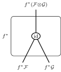
$$m_{[\mathcal{F},\mathcal{G}]}\colon f^{*}\mathcal{F}\otimes f^{*}\mathcal{G}\to f^{*}(\mathcal{F}\otimes\mathcal{G}).$$

Figure 3: Monoidal functor à la Melliès

The meaning of the box is that, inside, the $f^{*}$ is “stripped” from the objects; the name of the map $m_{[\mathcal{F},\mathcal{G}]}$ is not mentioned, as it is implicit to the diagram, which is specialized to the needs of monoidal categories. By comparision, the monoidality of $f^{*}$ may be expressed in our notation as in 4.

Figure 4: Monoidal functor in our notation

In each of its diagrams, the background layer is a horizontal string diagram with the strings being objects of the category corresponding to the planar region containing them (according to LABEL:string_diagram_transformation) and their intersections being transformations from left to right (here, marked, as we have no specialized notation for monoidal categories as we do for geofibered ones). Vertical stacking of objects’ strings corresponds to their monoidal product.

Unlike in the purely functorial diagrams, each individual diagram does not depict a morphism $m$; rather, it denotes the endpoints of such a morphism (the rightmost labeled object in each) and the “location” of $m$. The morphism itself is obtained by “sweeping” the functorial diagram over the objects from left to right, as shown above. Whenever it crosses a marked morphism, the motion corresponds to the introduction of that map between the “endpoint” on the left and the one on the right. (Obviously, we must forbid endpoint diagrams that would allow degenerate or ambiguous configurations.)

Thus, the diagrams display the history of an object and the potential natural morphisms, but it is the topological relationships between them that give the actual maps.

As a further example of this, consider the monoidality of the natural transformation $\theta=\operatorname{\mathsf{comp}}^{*}(g,f)$. In Melliès’ notation, it is the equation of diagrams in 5.

Figure 5: Monoidal transformation à la Melliès

The interpretation is straightforward; vertical juxtaposition of morphisms is composition and horizontal is monoidal product. In our notation, we express it in 6 as a closed loop of translations.

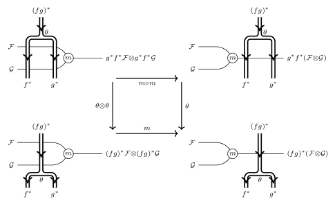
Figure 6: Monoidal transformation in our notation

Moving the functorial “foreground” from left to right, as before, produces one or two iterations of $m$, depending on how many of its strings cross that vertex. Moving the objects’ “background” from bottom to top produces an instance of the natural transformation $\operatorname{\mathsf{comp}}^{*}(f,g)$ (the one on the object $\mathcal{F}\otimes\mathcal{G}$ for the $\theta$ edge; for each factor of $\theta\otimes\theta$, we get the instances on $\mathcal{F}$ or $\mathcal{G}$ individually). Since the translational motions commute, so does the diagram of maps. We cannot help but feel that this is an instance of the Eckmann–Hilton argument for the commutativity of higher homotopy groups (as depicted in Hatcher’s book [hatcher]*p. 340).

The fact that we have expressed a single natural morphism, as in 4, in terms of an equivalence of several diagrams, would seem to be at odds with our intention of using individual diagrams to express natural transformations. In fact, this morphism could be expressed in a purely functorial notation with some additional convention as to the appearance of the “monoidal product string”, which would involve the complication of expressing its bivariant nature. However, it is actually this approach that is at odds with the philosophy of our diagrams, since the morphism of 4 is not a “structural” morphism but rather a “compatibility” between two independent structures. Moreover, the structures are not of an equivalent nature: the monoidal product is “internal” and the pullback functor (or any monoidal functor) is “external”. So it is entirely appropriate that their compatibility should be expressed through superimposed string diagrams of which one represents objects in the categories cut out by the other.

In summary: in this paper we have used “string diagrams” representing functors and their natural transformations, but we can “specialize” them to the corresponding values and their natural maps when applied to specific objects by superimposing such a diagram on a horizontal diagram of objects and morphisms in the categories cut out by the functorial diagram. Then any continuous motion (avoiding some degeneracies) “instantiates” the morphisms when the strings of one diagram cross the vertices of the other, and any closed loop should represent a commutative diagram of these maps.

We feel that this topological intuition is a valuable asset in a graphical algebraic notation, since it elevates the picture from simply a two-dimensional symbolic calculus to a genuinely graphical reasoning tool.