Huge thermoelectric effects in ferromagnet–superconductor junctions in the presence of a spin-splitting field

Abstract

We show that a huge thermoelectric effect can be observed by contacting a superconductor whose density of states is spin-split by a Zeeman field with a ferromagnet with a non-zero polarization. The resulting thermopower exceeds $k_{B}/e$ by a large factor, and the thermoelectric figure of merit $ZT$ can far exceed unity, leading to heat engine efficiencies close to the Carnot limit. We also show that spin-polarized currents can be generated in the superconductor by applying a temperature bias.

Thermoelectric effects, electric potentials generated by temperature gradients and vice versa, are intensely studied because of their possible use in converting the waste heat from various processes to useful energy. The conversion efficiency $\eta=\dot{W}/\dot{Q}$, the ratio of output power $\dot{W}$ to the rate of thermal energy consumed $\dot{Q}$, in thermoelectric devices however typically falls short of the theoretical Carnot limit and is low compared to other heat engines, which has motivated an extensive search for better materials. shakouri2011

In electronic conductors a major contributor to thermoelectricity is breaking of the symmetry between positive and negative-energy charge carriers (electrons and holes, respectively) ashcroftmermin . Within Sommerfeld expansion, this is described by the Mott relation cutler69 , which predicts thermoelectric effects of the order $\sim{}k_{B}T/E_{0}$, where $T$ is the temperature and $E_{0}$ a microscopic energy scale describing the energy dependence in the transport. This is usually a large atomic energy scale (in metals, the Fermi energy), so that $E_{0}\gg{}k_{B}T$ even at room temperature and these effects are often weak. Larger electron-hole asymmetries are however attainable in semiconductors, as the chemical potential can be tuned close to the band edges, where the density of states varies rapidly. shakouri2011 ; mahan1989-fmt

The situation in superconductors is superficially similar to semiconductors. The quasiparticle transport is naturally strongly energy dependent due to the presence of the energy gap $\Delta$, which can be significantly smaller than atomic energy scales. However, the chemical potential is not tunable in the same sense as in semiconductors, as charge neutrality dictates that electron-hole symmetry around the chemical potential is preserved. This implies that the thermoelectric effects in superconductors are often even weaker than in the corresponding normal state, in addition to being masked by supercurrents ginzburg44 ; galperin02 .

We show in this Letter that this problem can be overcome in a conventional superconductor by applying a spin-splitting field $h$. It shifts the energies of electrons with parallel and antiparallel spin orientations to opposite directions. Tedrow1971 This breaks the electron-hole symmetry for each spin separately, but conserves charge neutrality, as the total density of states remains electron-hole symmetric. In this situation, thermoelectric effects can be obtained by coupling the superconductor to a spin-polarized system.

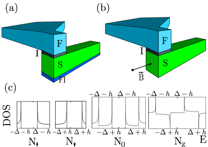
Figure 1: (Color online)Top: Schematic systems studied in this work. In both of them a ferromagnet (F) is coupled via a tunneling contact to a superconductor (S), whose tunneling density of states is modified by an exchange field. In (a) the exchange field is induced by the proximity of a ferromagnetic insulator (FI), whereas in (b) it is induced by the Zeeman energy due to an applied magnetic field $\vec{B}$ parallel with the easy axis of the ferromagnet. Bottom: Tunneling densities of states for spin $\uparrow/\downarrow$, averaged over spin ($N_{0}$), and the difference of them ($N_{z}$) obtained for an exchange field $h=\Delta/2$.

We propose that this effect can be realized in structures such as shown schematically in Fig. 1: There, a ferromagnet with a relatively large spin polarization is connected to a superconductor via a tunnel contact. Moreover, we assume the presence of a finite exchange field $h$ inside the superconductor. Such an exchange field can result from a Zeeman effect due to an applied magnetic field (Fig. 1b) Tedrow1971 , or from a magnetic proximity effect with either a ferromagnetic insulator Moodera1990 ; Moodera2013 ; Tokuyasu88 or with a thin ferromagnetic metallic layer Bergeret2001 ; giazotto07 placed directly below the superconductor (Fig. 1a). For simplicity, we assume this exchange field to be collinear with the magnetization inside the ferromagnet.

A standard tunneling Hamiltonian calculation yields for spin-$\sigma$ electrons from the ferromagnet the charge and heat currents

$$I_{\sigma} =\frac{G_{\sigma}}{e}\int_{-\infty}^{\infty}dEN_{\sigma}(E)[f_{F}(E)-f_{S}(E)]\,,$$ (1a)

$$\dot{Q}_{\sigma} =\frac{G_{\sigma}}{e^{2}}\int_{-\infty}^{\infty}dE(E-\mu_{F})N_{\sigma}(E)[f_{F}(E)-f_{S}(E)]\,.$$ (1b)

Here $N_{\uparrow/\downarrow}(E)=N_{S}(E\pm h)$ is the tunneling density of states (DOS) for spin $\uparrow/\downarrow$ particles divided by the normal-state density of states at Fermi energy, Tedrow1971 $N_{S}(E)=|E|/\sqrt{E^{2}-\Delta^{2}}\theta(|E|-\Delta)$ is the BCS DOS, $G_{\sigma}$ is the conductance through the junction for spin $\sigma$ particles in the normal state, and $f_{F/S}(E)$ are the (Fermi) distribution functions of electrons inside the ferromagnet and the superconductor, respectively. We disregard the energy dependence of the density of states inside the ferromagnet as well as the tiny electron-hole asymmetry possibly existing in the superconductor. Moreover, we fix the electrochemical potential of the superconductor to zero and describe the applied voltage via the potential $\mu_{F}=-eV$ in the ferromagnet.

The spin-dependent densities of states $N_{\sigma}(E)$ are plotted in Fig. 1c in the presence of a non-zero exchange field. We can see that they break the symmetry with respect to positive and negative energies for each spin. This symmetry breaking allows for the creation of a large spin-resolved thermoelectric effect, which can be converted to a spin-averaged effect via the spin filtering provided by the polarization $P\equiv(G_{\uparrow}-G_{\downarrow})/(G_{\uparrow}+G_{\downarrow})$. This can be seen better by introducing the charge and spin currents $I=I_{\uparrow}+I_{\downarrow}$ and $I_{S}=I_{\uparrow}-I_{\downarrow}$ as well as the heat and spin heat currents $\dot{Q}=\dot{Q}_{\uparrow}+\dot{Q}_{\downarrow}$ and $\dot{Q}_{S}=\dot{Q}_{\uparrow}-\dot{Q}_{\downarrow}$ along with $N_{0}\equiv(N_{\uparrow}+N_{\downarrow})/2$, $N_{z}\equiv N_{\uparrow}-N_{\downarrow}$,

$$I =\frac{G_{T}}{e}\int_{-\infty}^{\infty}dE\left[N_{0}+\frac{PN_{z}}{2}\right]\left[f_{F}-f_{S}\right]\,,$$ (2a)

$$I_{S} =\frac{G_{T}}{e}\int_{-\infty}^{\infty}dE\left[PN_{0}+\frac{N_{z}}{2}\right]\left[f_{F}-f_{S}\right]\,,$$ (2b)

$$\dot{Q} =\frac{G_{T}}{e^{2}}\int_{-\infty}^{\infty}dE(E-\mu_{F})\left[N_{0}+\frac{PN_{z}}{2}\right]\left[f_{F}-f_{S}\right]\,,$$ (2c)

$$\dot{Q}_{S} =\frac{G_{T}}{e^{2}}\int_{-\infty}^{\infty}dE(E-\mu_{F})\left[PN_{0}+\frac{N_{z}}{2}\right]\left[f_{F}-f_{S}\right]\,.$$ (2d)

Here $G_{T}=G_{\uparrow}+G_{\downarrow}$ is the conductance of the tunnel junction that would be measured in the absence of superconductivity. The average density of states $N_{0}(E)$ is symmetric and the difference $N_{z}(E)$ antisymmetric with respect to $E=0$ as shown in Fig. 1c. This means that they will pick up a different symmetry component of the distribution function difference in Eqs. (2) and eventually lead to a thermoelectric effect.

In order to grasp the size of the thermoelectric effects we assume either a small voltage $V$ or a small temperature difference $\Delta T/T=2(T_{L}-T_{R})/(T_{L}+T_{R})$ across the junctions and find the currents in Eqs. (2) up to linear order in $V$ and $\Delta T/T$. They can be written in a compact way, for the charge and heat currents

$$\begin{pmatrix}I\\ \dot{Q}\end{pmatrix}=\begin{pmatrix}G&P\alpha\\ P\alpha&G_{th}T\end{pmatrix}\begin{pmatrix}V\\ \Delta T/T\end{pmatrix}\;,$$ (3)

and for the spin and spin heat currents

$$\begin{pmatrix}I_{S}\\ \dot{Q}_{S}\end{pmatrix}=\begin{pmatrix}PG&\alpha\\ \alpha&PG_{th}T\end{pmatrix}\begin{pmatrix}V\\ \Delta T/T\end{pmatrix}\;.$$ (4)

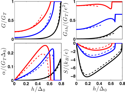
Figure 2: (Color online) Thermoelectric coefficients vs. exchange field $h$ at $k_{B}T/\Delta_{0}=0.1$ (black), 0.2 (blue) and 0.3 (red). From top left to bottom right: conductance, heat conductance, thermoelectric coefficient, and thermopower. The solid lines are numerical integrals of Eqs. (5), the dashed lines are the approximations in Eqs. (6,8). The curves have been calculated for $\Gamma=10^{-6}\Delta_{0}$. $\Delta_{0}$ is the superconducting order parameter at $T=0$ and $h=0$.

These response matrices are expressed in terms of three coefficients,

$$G =G_{T}\int_{-\infty}^{\infty}dE\frac{N_{0}(E)}{4k_{B}T\cosh^{2}\left(\frac{E}{2k_{B}T}\right)}\,,$$ (5a)

$$G_{th} =\frac{G_{T}}{e^{2}}\int_{-\infty}^{\infty}dE\frac{E^{2}N_{0}(E)}{4k_{B}T^{2}\cosh^{2}\left(\frac{E}{2k_{B}T}\right)}\,,$$ (5b)

$$\alpha =\frac{G_{T}}{2e}\int_{-\infty}^{\infty}dE\frac{EN_{z}(E)}{4k_{B}T\cosh^{2}\left(\frac{E}{2k_{B}T}\right)}\,.$$ (5c)

Besides the thermoelectric effect that is detailed below, we can already draw some important conclusions based on Eqs. (3-5): (i) The matrices in Eqs. (3-4) obey the Onsager reciprocal relations onsager31 ; jacquod12 ; machon13 , which for a generic thermoelectric response matrix $L$ describing response in a magnetic field $\vec{B}$ for magnetization $\vec{m}$ reads $L(\vec{B},\vec{m})=L^{T}(-\vec{B},-\vec{m})$. Moreover, the coefficients satisfy a thermodynamic stability condition $\alpha^{2}/(TGG_{\rm th})\leq 1$, due to Cauchy-Schwartz inequality. (ii) The thermoelectric effects vanish when $N_{z}=0$, i.e., when either no exchange field is applied ($h=0$) or when $\Delta=0$. Since $N_{z}(-h)=-N_{z}(h)$, inverting the exchange field changes the sign of the thermoelectric coefficients. It is important to emphasize that in order to get a non-zero spin-averaged thermoelectric effect, the spin polarization $P$ of the interface needs to be non-vanishing. (iii) According to Eq. (4), a finite spin-polarized current can flow if there is a temperature difference across the junction. This effect is the longitudinal analog to the spin-Seebeck effect observed in metallic magnets uchida2008 ; adachi2013 , and can here be found in a spin-splitting field even for a zero spin polarization $P=0$.

The response coefficients from Eqs. (5) are plotted as a function of exchange field $h$ in Fig. 2. We note that the thermoelectric coefficient $\alpha$ increases linearly for small $h$, and reaches a maximum for $h<\Delta_{0}$ (here, $\Delta_{0}$ is the superconducting order parameter at $T=0$ and $h=0$), and finally drops to zero when superconductivity is destroyed by $h$. Thermal conductance $G_{th}$ has a similar non-monotonic behavior, whereas the conductance G increases monotonically toward its normal-state value $G_{T}$. In the low temperature limit $k_{B}T\ll\Delta-|h|$, the coefficients can be approximated by

$$G \approx G_{T}\sqrt{2\pi\tilde{\Delta}}\cosh(\tilde{h})e^{-\tilde{\Delta}}\,,$$ (6a)

$$G_{\rm th} \approx\frac{k_{B}G_{T}\Delta}{e^{2}}\sqrt{\frac{\pi}{2\tilde{\Delta}}}e^{-\tilde{\Delta}}\left[e^{\tilde{h}}(\tilde{\Delta}-\tilde{h})^{2}+e^{-\tilde{h}}(\tilde{\Delta}+\tilde{h})^{2}\right]\,,$$ (6b)

$$\alpha \approx\frac{G_{T}}{e}\sqrt{2\pi\tilde{\Delta}}e^{-\tilde{\Delta}}\left[\Delta\sinh(\tilde{h})-h\cosh(\tilde{h})\right]\,,$$ (6c)

where $\tilde{\Delta}=\Delta/(k_{B}T)$ and $\tilde{h}=h/(k_{B}T)$. For $h=0$, the expressions reduce to the standard results for the NIS charge and heat conductance $G$ and $G_{\rm th}$, Nahum94 ; Leivo96 whereas $\alpha$ vanishes.

Instead of the thermally induced current, the typical thermoelectric observable is the thermopower or the Seebeck coefficient $S=-P\alpha/(GT)$, defined as the voltage $V$ observed due to a temperature difference $\Delta T$ after opening the circuit such that $I=0$. It can be obtained from Eqs. (5). The Seebeck coefficient for our FIS junction is plotted in the lower right panel of Fig. 2. The qualitative behavior is close to that of $\alpha$, but it is quantitatively changed by the $h$-dependence of $G$.

In the low temperature limit, $S$ can be obtained from Eqs. (6), $S\approx-\frac{P\Delta}{eT}[\tanh(\tilde{h})-h/\Delta]$. Thus, for low temperatures the thermopower is maximized for $h=k_{B}T{\rm arcosh}(\sqrt{\tilde{\Delta}})$, where

$$S_{\rm max}\approx-\frac{k_{B}}{e}P\left[\frac{\Delta}{k_{B}T}-{\rm arcosh}\left(\sqrt{\frac{\Delta}{k_{B}T}}\right)\right]\,,$$ (7)

It can hence greatly exceed $k_{B}/e$ and seems to diverge towards low temperatures as $1/T$. In practice this divergence is cut off by additional contributions beyond the standard BCS tunnel formula. These are often described via the phenomenological “broadening” parameter $\Gamma$ pekola04 . Practical reasons for the occurrence of an effectively non-zero $\Gamma$ are due to the fluctuations in the electromagnetic environment pekola10 , the presence of Andreev reflection rajauria08 ; laakso12 , or the inverse proximity effect from the ferromagnet sillanpaa01 ; kauppilaup13 . The main effect of the broadening parameter for the thermopower is to induce a finite density of states inside the gap that in turn leads to a correction of the charge conductance (6) of the order $\delta G=\frac{\Gamma}{\Delta}G_{T}$ (valid for $\Gamma\ll k_{B}T\ll\Delta$). The corrections for the other coefficients are less relevant. Within this limit we get for the thermopower

$$S =P\frac{\Delta}{eT}\frac{h\cosh\left(\frac{h}{k_{B}T}\right)-\Delta\sinh\left(\frac{h}{k_{B}T}\right)}{\Gamma e^{\Delta/(k_{B}T)}\sqrt{\frac{k_{B}T}{2\pi\Delta}}+\Delta\cosh\left(\frac{h}{k_{B}T}\right)}.$$ (8)

The result for $S$ is shown in the lower right panel of Fig. 2.

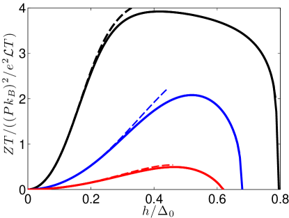
Figure 3: (Color online) Figure of merit ZT as a function of exchange field at $k_{B}T/\Delta_{0}=0.1$ (black), 0.2 (blue) and 0.3 (red) and $P=0.9$. The solid line is the exact result and the dashed line the result obtained from Eq. (9).

The power conversion ability of thermoelectric devices is usually characterized by a dimensionless figure of merit $ZT$, which can here be related to the junction parameters by $ZT=S^{2}GT/\tilde{G}_{\rm th}$, where $\tilde{G}_{\rm th}$ is the thermal conductance at zero current. foot At linear response, $\Delta T\ll{}T$, this determines the efficiency at maximum output power, $\eta=\eta_{CA}ZT/(ZT+2)$, where $\eta_{CA}=1-\sqrt{T_{\rm cold}/T_{\rm hot}}$ is the Curzon-Ahlborn efficiency. curzon1975 Best known thermoelectric bulk materials have $ZT\lesssim{}2$, but better efficiencies are achievable in nanostructures. shakouri2011

Assuming that the thermal conductance is dominated by the electronic contribution, we find at $k_{B}T\ll\Delta-|h|$

$$ZT=\frac{P^{2}}{1-P^{2}+\frac{\Delta^{2}}{\bigl{[}h\cosh\bigl{(}\frac{h}{k_{B}T}\bigr{)}-\Delta\sinh\bigl{(}\frac{h}{k_{B}T}\bigr{)}\bigr{]}^{2}}}\,,$$ (9)

which is shown and compared to numerical results in Fig. 3. For $k_{B}T\ll h$, we find $ZT=P^{2}/(1-P^{2})$. For $P\rightarrow 1$ (half-metal injector), $ZT$ approaches infinity, and the efficiency approaches theoretical upper bounds. From a practical point of view the main challenge in achieving large values for $ZT$ is the fabrication of barriers with large spin-polarization $P$.

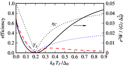
Figure 4: (Color online) Maximum power $\dot{W}=\max_{V}[-IV]$ generated by the FIS junction from a temperature difference $T_{F}-T_{S}$ (solid), and the corresponding heat engine efficiency $\eta$ (dashed). We fix $P=1.0$, $k_{B}T_{S}=0.2\Delta_{0}$, $h=0.6\Delta_{0}$, and $\Gamma=10^{-5}\Delta_{0}$. The linear-response result $\eta=\eta_{CA}ZT/(ZT+2)$ for $ZT=4.04$ and the Carnot efficiency $\eta_{C}=1-T_{\rm cold}/T_{\rm hot}$ are also shown (dotted).

Let us characterize the efficiency at larger temperature differences. Figure 4 shows the maximum extractable power as a function of the temperature difference, together with the conversion efficiency $\eta$. For a $1\,\mathrm{k\Omega}$ tunnel junction to aluminum, the maximum power in this figure corresponds to $\dot{W}\approx 1.5\,\mathrm{pW}$. The efficiency can be rather high, $\eta=0.7$, also when the extracted power is large.

Superconductors are known to support certain thermoelectric effects partly related to those discussed in this work. First, magnetic impurities in superconductors can break the electron-hole symmetry and lead to thermoelectric effects. kalenkov2012 Second, the cooling effect found in NIS junctions in the nonlinear regime is somewhat similar to the effect described here, if one substitutes the exchange field with a finite voltage $V\approx\Delta/e$ giazotto06 ; muhonen12 . Indeed, the extracted power found above is comparable to the maximum cooling power of a NIS junction. NIS junctions, however, cannot be used for power conversion, as their cooling power $\dot{Q}_{NIS}$ is a symmetric function of the bias voltage. The effect of ferromagnetism on NIS cooling was also discussed earlier, giazotto02 ; ozaeta2012 ; kawabata2013 but in those works the exchange field was introduced in order to suppress the Joule heating due to the Andreev current and did not affect the density of the states of the superconductor. According to our results the induced exchange field in the superconductor may lead to a larger cooling efficiency as in NIS junctions.

The results described above are obtained by assuming that the electron charge, spin and energy relax immediately after tunneling. This assumption can be lifted by considering the non-equilibrium state formed inside the ferromagnetic or the superconducting wire due to the biasing. This can be described by generalizing the quasiclassical Green’s function approach in Ref. morten04 to the case of a superconductor in a spin-splitting field, and describing the effect of the finite spin polarization inside the ferromagnet via an effective boundary condition derived in Ref. bergeret12 . We have verified that the effects described above are qualitatively not affected by such corrections. The details of this approach will be published elsewhere.

We also note that in the geometry of Fig. 1(b), where the Zeeman field is induced by a magnetic field, the orbital effect of the magnetic field will also influence the form of the density of states and for large fields it will eventually lead to a destruction of superconductivity. For simplicity, we have disregarded this effect in the above calculation. In practice, to minimize this effect, the magnetic field should be applied preferably in the longitudinal direction of the wire Meservey1970 , as depicted in Fig. 1(b).

Summarizing, we have shown that a junction between a conventional superconductor in the presence of an exchange field and a ferromagnet with polarization $P$ exhibits huge thermoelectric effects. The thermopower diverges at low temperatures in the absence of limiting effects, yielding a figure of merit $ZT\approx P^{2}/(1-P^{2})$ and heat engine efficiencies close to theoretical upper bounds. Moreover, even in the case of $P=0$ our model predicts finite spin currents in the presence of a temperature gradient, provided there is a spin-splitting of the density of states. These mechanisms in principle can work also in semiconductors without requiring doping which typically deteriorates the thermoelectric effects.

The authors thank V. Golovach for useful discussions. The work of F.S.B and A. O. have been supported by the Spanish Ministry of Economy and Competitiveness under Project FIS2011-28851-C02-02 and T.T.H. and P.V. by the Academy of Finland, the European Research Council (Grant No. 240362-Heattronics) and the EU-FP 7 INFERNOS (Grant No. 308850) program. The work of A. O. have also been supported by the CSIC and the European Social Fund under JAE-Predoc program and the EU-FP 7 MICROKELVIN project (Grant No. 228464). A.O. acknowledges the hospitality of O.V. Lounasmaa Laboratory (Aalto University), during his stay in Finland.

References

- (1) A. Shakouri, Annu. Rev. Mater. Res. 41, 399 (2011).
- (2) N.W. Ashcroft and D.N. Mermin, Solid State Physics (Saunders College, Philadelphia) (1976).
- (3) M. Cutler and N.F. Mott, Phys. Rev. 181, 1336 (1969).
- (4) G. D. Mahan, J. Appl. Phys. 65, 1578 (1989).
- (5) V.L. Ginsburg, Zh. Eksp. Teor. Fiz. 14, 134 (1944).
- (6) Y.M. Galperin, V.L. Gurevich, V.I. Kozub, and A.L. Shelankov, Phys. Rev. B 65, 064531 (2002).
- (7) P. M. Tedrow and R. Meservey, Phys. Rev. Lett. 27, 919 (1971).
- (8) X. Hao, J. S. Moodera, and R. Meservey, Phys. Rev. B 42, 8235 (1990).
- (9) Bin Li, N. Roschewsky, B. A. Assaf, M. Eich, M. Epstein-Martin, D. Heiman, M. Münzenberg, and J. S. Moodera, Phys. Rev. Lett. 110, 097001 (2013).
- (10) T. Tokuyasu, J. A. Sauls and D. Rainer, Phys. Rev. B 38, 8823 (1988).
- (11) F. S. Bergeret, A. F. Volkov and K. B. Efetov, Phys. Rev. Lett. 86, 3140 (2001).
- (12) F. Giazotto, F. Taddei, P. D’Amico, R. Fazio, and F. Beltram, Phys. Rev. B 76, 184518 (2007)
- (13) Lars Onsager, Phys. Rev. 38, 2265 (1931).
- (14) P. Jacquod, R.S. Whitney, J. Meair, and M. Büttiker, Phys. Rev. B 86, 155118 (2012).
- (15) P. Machon, M. Eschrig, and W. Belzig, Phys. Rev. Lett. 110, 047002 (2013).
- (16) H. Littman and B. Davidson, J. Appl. Phys. 32, 217 (1961).
- (17) K. Uchida, S. Takahashi, K. Harii, J. Ieda, W. Koshibae, K. Ando, S. Maekawa and E. Saitoh, Nature 455, 778 (2008).
- (18) H. Adachi, K. Uchida, E. Saitoh and S. Maekawa, Rep. Prog. Phys. 76, 036501 (2013).
- (19) M. Nahum, T. M. Eiles, and J. M. Martinis, Appl. Phys. Lett 65, 3123 (1994).
- (20) M. M. Leivo, J. P. Pekola and D. V. Averin, Appl. Phys. Lett. 68, 1996 (1996).
- (21) J.P. Pekola, T.T. Heikkilä, A.M. Savin, J.T. Flyktman, F. Giazotto, and F.W.J. Hekking, Phys. Rev. Lett. 92, 056804 (2004).
- (22) J.P. Pekola, V.F. Maisi, S. Kafanov, N. Chekurov, A. Kemppinen, Yu. A. Pashkin, O.-P. Saira, M. Möttönen, and J.S. Tsai, Phys. Rev. Lett. 105, 026803 (2010).
- (23) S. Rajauria, P. Gandit, T. Fournier, F. Hekking, B. Pan- netier, and H. Courtois, Phys. Rev. Lett. 100, 207002 (2008).
- (24) M.A. Laakso, T.T. Heikkilä, and Y. V. Nazarov, Phys. Rev. Lett. 108, 67002 (2012).
- (25) M.A. Sillanpää, T.T. Heikkilä, R.K. Lindell, and P.J. Hakonen, Europhys. Lett. 56, 590 (2001).
- (26) V.J. Kauppila, H.Q. Nguyen, and T.T. Heikkilä, arXiv:1304.1288.
- (27) T. S. Santos, J. S. Moodera, K. V. Raman, E. Negusse, J. Holroyd, J. Dvorak, M. Liberati, Y. U. Idzerda, and E. Arenholz, Phys. Rev. Lett. 101, 147201 (2008).
- (28) J. Morten, A. Brataas, and W. Belzig, Phys. Rev. B 70, 212508 (2004).
- (29) F.S. Bergeret, A. Verso, and A.F. Volkov, Phys. Rev. B 86, 214516 (2012).
- (30) A. Schmid and G. Schön, J. Low Temp. Phys. 20, 207 (1975).
- (31) K.D. Usadel, Phys. Rev. Lett. 25, 507 (1970).
- (32) R. Meservey, P. M. Tedrow and P. Fulde, Phys. Rev. Lett. 25, 1270 (1970).
- (33) F. Curzon and B. Ahlborn, Am. J. Phys. 43, 22 (1975); P. Chambadal, Les Centrales Nuclaires (Armand Colin, Paris, 1957); I.I. Novikov, At. Energy (N.Y.) 3, 1269 (1957); J. Nucl. Energy 7, 125 (1958).
- (34) M. S. Kalenkov, A. D. Zaikin, L. S. Kuzmin, Phys. Rev. Lett. 109, 147004 (2012).
- (35) F. Giazotto, T.T. Heikkilä, A. Luukanen, A.M. Savin, and J.P. Pekola, Rev. Mod. Phys. 78, 217 (2006).
- (36) J.T. Muhonen, M. Meschke, and J.P. Pekola, Rep. Progr. Phys. 75, 046501 (2012).
- (37) F. Giazotto, F. Taddei, R. Fazio, and F. Beltram, Appl. Phys. Lett. 80, 3784 (2002).
- (38) A. Ozaeta, A. S. Vasenko, F. W. J. Hekking, and F. S. Bergeret, Phys. Rev. B 85, 174518 (2012).
- (39) S. Kawabata, A. Ozaeta, A. S. Vasenko, F. W. J. Hekking, and F. S. Bergeret, Appl. Phys. Lett. 103, 032602 (2013).
- (40) The thermal conductance at zero current is related with at zero voltage difference [cf. Eqs. (3-4)] by the expression . littman1961