Abstract

We study the problem of learning a tensor from a set of linear measurements. A prominent methodology for this problem is based on a generalization of trace norm regularization, which has been used extensively for learning low rank matrices, to the tensor setting. In this paper, we highlight some limitations of this approach and propose an alternative convex relaxation on the Euclidean ball. We then describe a technique to solve the associated regularization problem, which builds upon the alternating direction method of multipliers. Experiments on one synthetic dataset and two real datasets indicate that the proposed method improves significantly over tensor trace norm regularization in terms of estimation error, while remaining computationally tractable.

1 Introduction

During the recent years, there has been a growing interest on the problem of learning a tensor from a set of linear measurements, such as a subset of its entries, see [9, 17, 22, 23, 25, 26, 27] and references therein. This methodology, which is also referred to as tensor completion, has been applied to various fields, ranging from collaborative filtering [15], to computer vision [17], to medical imaging [9], among others. In this paper, we propose a new method to tensor completion, which is based on a convex regularizer which encourages low rank tensors and develop an algorithm for solving the associated regularization problem.

Arguably the most widely used convex approach to tensor completion is based upon the extension of trace norm regularization [24] to that context. This involves computing the average of the trace norm of each matricization of the tensor [16]. A key insight behind using trace norm regularization for matrix completion is that this norm provides a tight convex relaxation of the rank of a matrix defined on the spectral unit ball [8]. Unfortunately, the extension of this methodology to the more general tensor setting presents some difficulties. In particular, we shall prove in this paper that the tensor trace norm is not a tight convex relaxation of the tensor rank.

The above negative result stems from the fact that the spectral norm, used to compute the convex relaxation for the trace norm, is not an invariant property of the matricization of a tensor. This observation leads us to take a different route and study afresh the convex relaxation of tensor rank on the Euclidean ball. We show that this relaxation is tighter than the tensor trace norm, and we describe a technique to solve the associated regularization problem. This method builds upon the alternating direction method of multipliers and a subgradient method to compute the proximity operator of the proposed regularizer. Furthermore, we present numerical experiments on one synthetic dataset and two real-life datasets, which indicate that the proposed method improves significantly over tensor trace norm regularization in terms of estimation error, while remaining computationally tractable.

The paper is organized in the following manner. In Section 2, we describe the tensor completion framework. In Section 3, we highlight some limitations of the tensor trace norm regularizer and present an alternative convex relaxation for the tensor rank. In Section 4, we describe a method to solve the associated regularization problem. In Section 5, we report on our numerical experience with the proposed method. Finally, in Section 6, we summarize the main contributions of this paper and discuss future directions of research.

2 Preliminaries

In this section, we begin by introducing some notation and then proceed to describe the learning problem. We denote by ${\mathbb{N}}$ the set of natural numbers and, for every $k\in{\mathbb{N}}$, we define $[k]=\{1,\dots,k\}$. Let ${N}\in{\mathbb{N}}$ and let ${p}_{1},\dots,{p}_{N}\geq 2$. An ${N}$-order tensor ${\boldsymbol{\cal W}}\in{\mathbb{R}}^{{p}_{1}\times\cdots\times{p}_{N}}$, is a collection of real numbers $({{\cal W}}_{i_{1},\dots,i_{N}}:i_{n}\in[{p}_{n}],n\in[{N}])$. Boldface Euler scripts, e.g. ${\boldsymbol{\cal W}}$, will be used to denote tensors of order higher than two. Vectors are $1$-order tensors and will be denoted by lower case letters, e.g. $x$ or $a$; matrices are $2$-order tensors and will be denoted by upper case letters, e.g. $W$. If $x\in{\mathbb{R}}^{d}$ then for every $r\leq s\leq d$, we define $x_{r:s}:=(x_{i}:r\leq i\leq s)$. We also use the notation $p_{\min}=\min\{p_{1},\ldots,p_{N}\}$ and $p_{\max}=\max\{p_{1},\ldots,p_{N}\}$.

A mode-$n$ fiber of a tensor ${\boldsymbol{\cal W}}$ is a vector composed of the elements of ${\boldsymbol{\cal W}}$ obtained by fixing all indices but one, corresponding to the $n$-th mode. This notion is a higher order analogue of columns (mode-$1$ fibers) and rows (mode-$2$ fibers) for matrices. The mode-$n$ matricization (or unfolding) of ${\boldsymbol{\cal W}}$, denoted by $W_{\left(n\right)}$, is a matrix obtained by arranging the mode-$n$ fibers of ${\boldsymbol{\cal W}}$ so that each of them is a column of $W_{\left(n\right)}\in\mathbb{R}^{{p}_{n}\times J_{n}}$, where $J_{n}:=\prod_{k\neq n}{p}_{k}$. Note that the order of the columns is not important as long as it is consistent.

We are now ready to describe the learning problem. We choose a linear operator ${\cal I}:{\mathbb{R}}^{{p}_{1}\times\cdots\times{p}_{N}}\rightarrow{\mathbb{R}}^{m}$, representing a set of linear measurements obtained from a target tensor ${\boldsymbol{\cal W}}^{0}$ as $y={\cal I}({\boldsymbol{\cal W}}^{0})+\xi$, where $\xi$ is some disturbance noise. In this paper, we mainly focus on tensor completion, in which case the operator ${\cal I}$ measures elements of the tensor. That is, we have ${\cal I}({\boldsymbol{\cal W}}^{0})=({\boldsymbol{\cal W}}^{0}_{i_{1}(j),\dots,i_{N}(j)}:j\in[m])$, where, for every $j\in[m]$ and $n\in[N]$, the index $i_{n}(j)$ is a prescribed integer in the set $[p_{n}]$. Our aim is to recover the tensor ${\boldsymbol{\cal W}}^{0}$ from the data $({\cal I},y)$. To this end, we solve the regularization problem

$$\min\big{\{}\|y-{\cal I}({\boldsymbol{\cal W}})\|^{2}_{2}+\gamma R({\boldsymbol{\cal W}}):{{\boldsymbol{\cal W}}\in{\mathbb{R}}^{{p}_{1}\times\cdots\times{p}_{N}}}\big{\}}$$ (1)

where $\gamma$ is a positive parameter which may be chosen by cross validation. The role of the regularizer $R$ is to encourage tensors ${\boldsymbol{\cal W}}$ which have a simple structure in the sense that they involve a small number of “degrees of freedom”. A natural choice is to consider the average of the rank of the tensor’s matricizations. Specifically, we consider the combinatorial regularizer

$$R({\boldsymbol{\cal W}})=\frac{1}{N}\sum\limits_{n=1}^{N}{\rm rank}(W_{(n)}).$$ (2)

Finding a convex relaxation of this regularizer has been the subject of recent works [9, 17, 23]. They all agree to use the trace norm for tensors as a convex proxy of $R$. This is defined as the average of the trace norm of each matricization of ${\boldsymbol{\cal W}}$, that is,

$$\|{\boldsymbol{\cal W}}\|_{\rm tr}=\frac{1}{N}\sum\limits_{n=1}^{N}\|W_{\left(n\right)}\|_{\rm tr}$$ (3)

where $\|W_{(n)}\|_{\rm tr}$ is the trace (or nuclear) norm of matrix $W_{(n)}$, namely the $\ell_{1}$-norm of the vector of singular values of matrix $W_{(n)}$ (see, e.g. [14]). Note that in the particular case of $2$-order tensors, functions (2) and (3) coincide with the usual notion of rank and trace norm of a matrix, respectively.

A rational behind the regularizer (3) is that the trace norm is the tightest convex lower bound to the rank of a matrix on the spectral unit ball, see [8, Thm. 1]. This lower bound is given by the convex envelope of the function

$$\Psi(W)=\left\{\begin{array}[]{ll}{\rm rank}(W),&\text{if }\|W\|_{\infty}\leq 1\\ +\infty,&\text{otherwise}\end{array}\right.$$ (4)

where $\|\cdot\|_{\infty}$ is the spectral norm, namely the largest singular value of $W$. The convex envelope can be derived by computing the double conjugate of $\Psi$. This is defined as

$$\Psi^{**}(W)=\sup\left\{{\langle}W,S{\rangle}-\Psi^{*}(W):S\in{\mathbb{R}}^{p_{1}\times p_{2}}\right\}$$ (5)

where $\Psi^{*}$ is the conjugate of $\Psi$, namely $\Psi^{*}(S)=\sup\left\{{\langle}W,S{\rangle}-\Psi(W):W\in{\mathbb{R}}^{p_{1}\times p_{2}}\right\}$.

Note that $\Psi$ is a spectral function, that is, $\Psi(W)=\psi(\sigma(W))$ where $\psi:{\mathbb{R}}_{+}^{d}\rightarrow{\mathbb{R}}$ denotes the associated symmetric gauge function. Using von Neumann’s trace theorem (see e.g. [14]) it is easily seen that $\Psi^{*}(S)$ is also a spectral function. That is, $\Psi^{*}(S)=\psi^{*}(\sigma(S))$, where

$$\psi^{*}(\sigma)=\sup\left\{{\langle}\sigma,w{\rangle}-\psi(w):w\in{\mathbb{R}}_{+}^{d}\right\},~{}~{}~{}{\rm with~{}}d:=\min(p_{1},p_{2}).$$

We refer to [8] for a detailed discussion of these ideas. We will use this equivalence between spectral and gauge functions repeatedly in the paper.

3 Alternative Convex Relaxation

In this section, we show that the tensor trace norm is not a tight convex relaxation of the tensor rank $R$ in equation (2). We then propose an alternative convex relaxation for this function.

Note that due to the composite nature of the function $R$, computing its convex envelope is a challenging task and one needs to resort to approximations. In [22], the authors note that the tensor trace norm $\|\cdot\|_{\rm tr}$ in equation (3) is a convex lower bound to $R$ on the set

$$\mathcal{G}_{{\rm\infty}}:=\left\{\boldsymbol{{{\boldsymbol{\cal W}}}}\in\mathbb{R}^{p_{1}\times\cdots\times p_{N}}\,:\,\left\|W_{\left(n\right)}\right\|_{{\rm\infty}}\leq 1,~{}\forall n\in[N]\right\}.$$

The key insight behind this observation is summarized in Lemma 4, which we report in Appendix A. However, the authors of [22] leave open the question of whether the tensor trace norm is the convex envelope of $R$ on the set $\mathcal{G}_{{\rm\infty}}$. In the following, we will prove that this question has a negative answer by showing that there exists a convex function $\Omega\neq\|\cdot\|_{\rm tr}$ which underestimates the function $R$ on $\mathcal{G}_{{\rm\infty}}$ and such that for some tensor ${\boldsymbol{\cal W}}\in\mathcal{G}_{{\rm\infty}}$ it holds that $\Omega({\boldsymbol{\cal W}})>\|{\boldsymbol{\cal W}}\|_{\rm tr}$.

To describe our observation we introduce the set

$$\mathcal{G}_{{\rm 2}}:=\left\{{\boldsymbol{\cal W}}\in\mathbb{R}^{p_{1}\times\ldots\times p_{N}}:\|{\boldsymbol{\cal W}}\|_{2}\leq 1\right\}$$

where $\|\cdot\|_{2}$ is the Euclidean norm for tensors, that is,

$$\|{\boldsymbol{\cal W}}\|_{2}^{2}:=\sum_{i_{1}=1}^{p_{1}}\cdots\sum_{i_{N}=1}^{p_{N}}({{\cal W}}_{i_{1},\dots,i_{N}})^{2}.$$

We will choose

$$\Omega({\boldsymbol{\cal W}})=\Omega_{\alpha}({\boldsymbol{\cal W}}):=\frac{1}{N}\sum_{n=1}^{N}\omega^{**}_{\alpha}\left(\sigma\left(W_{(n)}\right)\right)$$ (6)

where $\omega_{\alpha}^{**}$ is the convex envelope of the cardinality of a vector on the $\ell_{2}$-ball of radius $\alpha$ and we will choose $\alpha=\sqrt{p_{{\rm min}}}$. Note, by Lemma 4 stated in Appendix A, that, for every $\alpha>0$, function $\Omega_{\alpha}$ is a convex lower bound of function $R$ on the set $\alpha\hskip 0.85355pt\mathcal{G}_{{\rm 2}}$.

Below, for every vector $s\in{\mathbb{R}}^{d}$ we denote by $s^{\downarrow}$ the vector obtained by reordering the components of $s$ so that they are non increasing in absolute value, that is, $|s^{\downarrow}_{1}|\geq\cdots\geq|s^{\downarrow}_{d}|$.

Lemma 1.

Let $\omega^{**}_{\alpha}$ be the convex envelope of the cardinality function on the $\ell_{2}$-ball of radius $\alpha$. Then, for every $x\in{\mathbb{R}}^{d}$ such that $\|x\|_{2}=\alpha$, it holds that $\omega_{\alpha}^{**}\left(x\right)={\rm card}\left(x\right)$.

Proof.

First, we note that the conjugate of the function ${\rm card}$ on the $\ell_{2}$ ball of radius $\alpha$ is given by the formula

$$\omega_{\alpha}^{*}\left(s\right)=\underset{\|y\|_{2}\leq\alpha}{{\rm sup}}\{{\langle}s,y{\rangle}-{\rm card}\left(y\right)\}=\underset{r\in\left\{0,\ldots,d\right\}}{\max}\{\alpha\|s^{\downarrow}_{1:r}\|_{2}-r\}.$$ (7)

Hence, by the definition of the double conjugate, we have, for every $s\in{\mathbb{R}}^{d}$ that

$$\omega_{\alpha}^{**}\left(x\right)\geq{\langle}s,x{\rangle}-\underset{r\in\left\{0,\ldots,d\right\}}{{\rm max}}\{\alpha\|s^{\downarrow}_{1:r}\|_{2}-r\}.$$

In particular, if $s=kx$ for some $k>0$ this inequality becomes

$$\omega_{\alpha}^{**}(x)\geq k\|x\|_{2}^{2}-\underset{r\in\left\{0,\ldots,d\right\}}{\max}(\alpha k\|x^{\downarrow}_{1:r}\|_{2}-r).$$

If $k$ is large enough, the maximum is attained at $r={\rm card}(x)$. Consequently,

$$\omega_{\alpha}^{**}(x)\geq k\alpha^{2}-k\alpha^{2}+{\rm card}(x)={\rm card}(x).$$

By the definition of the convex envelope, it also holds that $\omega_{\alpha}^{**}(x)\leq{\rm card}(x)$. The result follows. ∎

The next lemma provides, together with Lemma 1, a sufficient condition for the existence of a tensor ${\boldsymbol{\cal W}}\in{\cal G}_{\rm\infty}$ at which the proposed regularizer is strictly larger than the tensor trace norm.

Lemma 2.

If $N\geq 3$ and $p_{1},\dots,p_{N}$ are not all equal to each other, then there exists ${\boldsymbol{\cal W}}\in{\mathbb{R}}^{p_{1}\times\cdots\times p_{N}}$ such that: (a) $\|{\boldsymbol{\cal W}}\|_{2}=\sqrt{p_{\min}}$, (b) ${\boldsymbol{\cal W}}\in{\cal G}_{\rm\infty}$, (c) $\min\limits_{n\in[N]}{\rm rank}(W_{(n)})<\max\limits_{n\in[N]}{\rm rank}(W_{(n)})$.

Proof.

Without loss of generality we assume that $p_{1}\leq\cdots\leq p_{N}$. By hypothesis $p_{1}<p_{N}$. First we consider the special case

$$p_{1}=\dots=p_{N-1},~{}{\rm and}\hskip 1.42271pt~{}p_{N}=p_{1}+1.$$ (8)

We define a class of tensors ${\boldsymbol{\cal W}}$ by choosing a singular value decomposition for their mode-$N$ matricization,

$${{\cal W}}_{i_{1},i_{2},\dots,i_{N}}=\sum_{k=1}^{p_{N}}\sigma_{k}u^{k}_{i_{N}}v^{k}_{i_{1},\dots,i_{N-1}}$$ (9)

where $\sigma_{1}=\cdots=\sigma_{p_{N}}=\sqrt{p_{1}/(p_{1}+1)}$, the vectors $u^{k}\in{\mathbb{R}}^{p_{N}},\forall k\in[p_{N}]$ are orthonormal and the vectors $v^{k}\in{\mathbb{R}}^{p_{1}p_{2}\cdots p_{N-1}},\forall k\in[p_{N}]$ are orthonormal as well. Moreover, we choose $v^{k}$ as

$$v^{k}_{i_{1},\dots,i_{N-1}}=\left\{\begin{array}[]{cll}1&~{}\text{if }i_{1}=\cdots=i_{N-1}=k,&~{}k<p_{N}\\ \frac{1}{\sqrt{p_{1}}}&~{}\text{if }i_{2}=\cdots=i_{N-1}={\rm module}(i_{1},p_{1})+1,&~{}k=p_{N}\\ 0&~{}\text{otherwise}.&\end{array}\right.$$ (10)

By construction the matrix $W_{(N)}$ has rank equal to $p_{N}$ and Frobenius norm equal to $\sqrt{p_{1}}$. Thus properties (a) and (c) hold true. It remains to show that ${\boldsymbol{\cal W}}$ satisfies property (b). To this end, we will show, for every $n\in[N]$ and every $x\in{\mathbb{R}}^{p_{n}}$, that

$$\|W_{(n)}^{\scriptscriptstyle\top}x\|_{2}\leq\|x\|_{2}.$$

The case $n=N$ is immediate. If $n=1$ we have

$$\|W_{(1)}^{\scriptscriptstyle\top}x\|_{2}^{2} = \sum_{i_{2},\dots,i_{N}}\left(\sum_{k}\sigma_{k}\sum_{i_{1}}u^{k}_{i_{N}}v^{k}_{i_{1},\dots,i_{N-1}}x_{i_{1}}\right)^{2}$$

$$= \sum_{i_{2},\dots,i_{N}}\sum_{k,\ell}\sum_{i_{1},j_{1}}x_{i_{1}}x_{j_{1}}\sigma_{k}\sigma_{\ell}u^{k}_{i_{N}}u^{\ell}_{i_{N}}v^{k}_{i_{1},i_{2},\dots,i_{N-1}}v^{\ell}_{j_{1},i_{2},\dots,i_{N-1}}$$

$$= \sum_{k}\sigma_{k}^{2}\sum_{i_{1},j_{1}}x_{i_{1}}x_{j_{1}}\left(\sum_{i_{2},\dots,i_{N-1}}v^{k}_{i_{1},i_{2},\dots,i_{N-1}}v^{k}_{j_{1},i_{2},\dots,i_{N-1}}\right)$$

$$= \sum_{k}\sigma_{k}^{2}x_{k}^{2}+\frac{\sigma_{p_{N}}^{2}}{p_{1}}\sum_{k}x_{k}^{2}=\|x\|_{2}^{2}$$

where we used $\sum_{i_{N}}u^{k}_{i_{N}}u^{\ell}_{i_{N}}=\delta_{k,\ell}$ in the third equality, equation (10) and a direct computation in the fourth equality, and the definition of $\sigma_{k}$ in the last equality.
All other cases, namely $n=2,\dots,N-1$, are conceptually identical, so we only discuss the case $n=2$. We have

$$\|W_{(2)}^{\scriptscriptstyle\top}x\|_{2}^{2} = \sum_{i_{1},i_{3},\dots,i_{N}}\left(\sum_{k}\sigma_{k}\sum_{i_{2}}u^{k}_{i_{N}}v^{k}_{i_{2},\dots,i_{N-1}}x_{i_{2}}\right)^{2}$$

$$= \sum_{i_{1},i_{3},\dots,i_{N}}\sum_{k,\ell}\sum_{i_{2},j_{2}}x_{i_{2}}x_{j_{2}}\sigma_{k}\sigma_{\ell}u^{k}_{i_{N}}u^{\ell}_{i_{N}}v^{k}_{i_{1},i_{2},\dots,i_{N-1}}v^{\ell}_{i_{1},j_{2},\dots,i_{N-1}}$$

$$= \sum_{k}\sigma_{k}^{2}\sum_{i_{2},j_{2}}\left(x_{i_{2}}x_{j_{2}}\sum_{i_{1},i_{3},\dots,i_{N=1}}v^{k}_{i_{1},i_{2},\dots,i_{N-1}}v^{k}_{i_{1},j_{2},\dots,i_{N-1}}\right)$$

$$= \sum_{k}\sigma_{k}^{2}x_{k}^{2}+\frac{\sigma_{p_{N}}^{2}}{p_{1}}\sum_{k}x_{k}^{2}=\|x\|_{2}^{2}$$

where again we used $\sum_{i_{N}}u^{k}_{i_{N}}u^{\ell}_{i_{N}}=\delta_{k,\ell}$ in the third equality, equation (10) and a direct computation in the fourth equality, and the definition of $\sigma_{k}$ in the last equality.
Finally, if assumption (8) is not true we set ${{\cal W}}_{i_{1},\dots,i_{N}}=0$ if $i_{n}\geq p_{1}+1$, for some $n\leq N-1$ or $i_{N}>p_{1}+1$. We then proceed as in the case $p_{1}=\dots=p_{N-1}$ and $p_{N}=p_{1}+1$. ∎

We are now ready to present the main result of this section.

Proposition 3.

Let $p_{1},\dots,p_{N}\in{\mathbb{N}}$, let $\|\cdot\|_{\rm tr}$ be the tensor trace norm in equation (3) and let $\Omega_{\alpha}$ be the function in equation (6) for $\alpha=\sqrt{p_{\min}}$. If $p_{\min}<p_{\max}$, then there are infinitely many tensors ${\boldsymbol{\cal W}}\in{\cal G}_{{\rm\infty}}$ such that $\Omega_{\alpha}({\boldsymbol{\cal W}})>\|{\boldsymbol{\cal W}}\|_{\rm tr}$. Moreover, for every ${\boldsymbol{\cal W}}\in{\cal G}_{{\rm 2}}$, it holds that $\Omega_{1}({\boldsymbol{\cal W}})\geq\|{\boldsymbol{\cal W}}\|_{\rm tr}$.

Proof.

By construction $\Omega_{\alpha}({\boldsymbol{\cal W}})\leq R({\boldsymbol{\cal W}})$ for every ${\boldsymbol{\cal W}}\in\alpha{\cal G}_{2}$. Since ${\cal G}_{{\rm\infty}}\subset\alpha\mathcal{G}_{{\rm 2}}$ then $\Omega_{\alpha}$ is a convex lower bound for the tensor rank $R$ on the set $\mathcal{G}_{{\rm\infty}}$ as well. The first claim now follows by Lemmas 1 and 2. Indeed, all tensors obtained following the process described in Lemma 2 have the property that

$$\|{\boldsymbol{\cal W}}\|_{\rm tr} = \frac{1}{N}\sum_{n=1}^{N}\|\sigma(W_{(n)})\|_{1}$$

$$= \frac{1}{N}\left(p_{{\rm min}}(N-1)+\sqrt{p_{\min}^{2}+p_{\min}}\right)$$

$$< \frac{1}{N}\left(p_{\min}(N-1)+p_{\min}+1\right)=\Omega({\boldsymbol{\cal W}})=R({\boldsymbol{\cal W}}).$$

Furthermore there are infinitely many such tensors which satisfy this claim since the left singular vectors can be arbitrarily chosen in equation (9).
To prove the second claim, we note that since $\omega_{1}^{**}$ is the convex envelope of the cardinality ${\rm card}$ on the Euclidean unit ball, then it holds that $\omega_{1}^{**}(\sigma)\geq\|\sigma\|_{1}$ for every vector $\sigma$ such that $\|\sigma\|_{2}\leq 1$. Consequently,

$$\Omega_{1}({\boldsymbol{\cal W}})=\frac{1}{N}\sum_{n=1}^{N}\omega_{1}^{**}\left(\sigma\left(W_{(n)}\right)\right)\geq\frac{1}{N}\sum_{n=1}^{N}\|\sigma(W_{(n)})\|_{1}=\|{\boldsymbol{\cal W}}\|_{\rm tr}.$$

∎

The above result stems from the fact that the spectral norm is not an invariant property of the matricization of a tensor, whereas the Euclidean (Frobenius) norm is. This observation leads us to further study the function $\Omega_{\alpha}$.

4 Optimization Method

In this section, we explain how to solve the regularization problem associated with the proposed regularizer (6). For this purpose, we first recall the alternating direction method of multipliers (ADMM) [4], which was conveniently applied to tensor trace norm regularization in [9, 22].

4.1 Alternating Direction Method of Multipliers (ADMM)

To explain ADMM we consider a more general problem comprising both tensor trace norm regularization and the regularizer we propose,

$$\underset{\boldsymbol{{\cal W}}}{{\rm min}}\left\{E\left(\boldsymbol{{\cal W}}\right)+\gamma\underset{n=1}{\overset{N}{\sum}}\Psi\left(W_{(n)}\right)\right\}$$ (11)

where $E({\boldsymbol{\cal W}})$ is an error term such as $\|y-{\cal I}({\boldsymbol{\cal W}})\|^{2}_{2}$ and $\Psi$ is a convex spectral function. It is defined, for every matrix $A$, as

$$\Psi(A)=\psi(\sigma(A))$$

where $\psi$ is a gauge function, namely a function which is symmetric and invariant under permutations. In particular, if $\psi$ is the $\ell_{1}$ norm then problem (11) corresponds to tensor trace norm regularization, whereas if $\psi=\omega^{**}_{\alpha}$ it implements the proposed regularizer.

Problem (11) poses some difficulties because the terms under the summation are interdependent, that is, the different matricizations of ${\boldsymbol{\cal W}}$ have the same elements rearranged in a different way. In order to overcome this difficulty, the authors of [9, 22] proposed to use ADMM as a natural way to decouple the regularization term appearing in problem (11). This strategy is based on the introduction of $N$ auxiliary tensors, $\boldsymbol{{\cal B}}_{1},\ldots,\boldsymbol{{\cal B}}_{N}\in\mathbb{R}^{p_{1}\times\cdots\times p_{N}}$, so that problem (11) can be reformulated as

$$\underset{\mathbf{\boldsymbol{{\cal W}}},\boldsymbol{{\cal B}}_{1},\ldots,\mathbf{\boldsymbol{{\cal B}}}_{N}}{{\rm min}}\left\{\frac{1}{\gamma}E\left(\boldsymbol{{\cal W}}\right)+\underset{n=1}{\overset{N}{\sum}}\Psi\left(B_{n(n)}\right)\,\,:~{}\mathbf{\boldsymbol{{\cal B}}}_{n}=\boldsymbol{{\cal W}},\,n\in\left[N\right]\right\}$$ (12)

The corresponding augmented Lagrangian (see e.g. [4, 5]) is given by

$$\mathcal{L}\left(\boldsymbol{{\cal W}},\boldsymbol{{\cal B}},\boldsymbol{{\cal A}}\right)=\frac{1}{\gamma}E\left(\boldsymbol{{\cal W}}\right)+\underset{n=1}{\overset{N}{\sum}}\left(\Psi\left(B_{n(n)}\right)-\left\langle\boldsymbol{{\cal A}}_{n},\boldsymbol{{\cal W}}-\mathbf{\boldsymbol{{\cal B}}}_{n}\right\rangle+\frac{\beta}{2}\left\|\boldsymbol{{\cal W}}-\boldsymbol{{\cal B}}_{n}\right\|_{2}^{2}\right),$$ (13)

where ${\langle}\cdot,\cdot{\rangle}$ denotes the scalar product between tensors, $\beta$ is a positive parameter and $\boldsymbol{{\cal A}}_{1},\ldots\boldsymbol{{\cal A}}_{N}\in{\mathbb{R}}^{p_{1}\times\cdots\times p_{N}}$ are the set of Lagrange multipliers associated with the constraints in problem (12).

ADMM is based on the following iterative scheme

$$\boldsymbol{{\cal W}}^{\left[i+1\right]} \leftarrow \underset{\boldsymbol{{\cal W}}}{{\rm argmin}}~{}\mathcal{L}\left(\boldsymbol{{\cal W}},\boldsymbol{{\cal B}}^{[i]},\boldsymbol{{\cal A}}^{[i]}\right)$$ (14)

$$\boldsymbol{{\cal B}}_{n}^{\left[i+1\right]} \leftarrow \underset{\boldsymbol{{\cal B}}_{n}}{{\rm argmin}}~{}\mathcal{L}\left(\boldsymbol{{\cal W}}^{\left[i+1\right]},\boldsymbol{{\cal B}},\boldsymbol{{\cal A}}^{[i]}\right)$$ (15)

$$\boldsymbol{{\cal A}}_{n}^{\left[i+1\right]} \leftarrow \boldsymbol{{\cal A}}_{n}^{\left[i\right]}-\left(\beta\boldsymbol{{\cal W}}^{\left[i+1\right]}-\boldsymbol{{\cal B}}_{n}^{\left[i+1\right]}\right).$$ (16)

Step (16) is straightforward, whereas step (14) is described in [9]. Here we focus on the step (15) since this is the only problem which involves function $\Psi$. We restate it with more explanatory notations as

$$\underset{B_{n(n)}}{\rm argmin}\left\{\Psi\left(B_{n(n)}\right)-\left\langle A_{n(n)},W_{(n)}-B_{n(n)}\right\rangle+\frac{\beta}{2}\left\|W_{(n)}-B_{n(n)}\right\|_{2}^{2}\right\}.$$

By completing the square in the right hand side, the solution of this problem is given by

$$\hat{B}_{n(n)}={\rm prox}_{\frac{1}{\beta}\Psi}\left(X\right):=\underset{B_{n(n)}}{{\rm argmin}}\left\{\frac{1}{\beta}\Psi\left(B_{n(n)}\right)+\frac{1}{2}\left\|B_{n(n)}-X\right\|_{2}^{2}\right\}$$

where $X=W_{\left(n\right)}-\frac{1}{\beta}A_{n\left(n\right)}$. By using properties of proximity operators (see e.g. [2, Prop. 3.1]) we know that if $\psi$ is a gauge function then

$${\rm prox}_{\frac{1}{\beta}\Psi}\left(X\right)=U_{X}{\rm diag\left({\rm prox}_{\frac{1}{\beta}\psi}\left(\sigma(X)\right)\right)}V_{X}^{\top}$$

where $U_{X}$ and $V_{X}$ are the orthogonal matrices formed by the left and right singular vectors of $X$, respectively.

If we choose $\psi=\left\|\cdot\right\|_{1}$ the associated proximity operator is the well-known soft thresholding operator, that is, ${\rm prox}_{\frac{1}{\beta}\left\|\cdot\right\|_{1}}\left(\sigma\right)=v$, where the vector $v$ has components

$$v_{i}={\rm sign}\left(\sigma_{i}\right)\left(\left|\sigma_{i}\right|-\frac{1}{\beta}\right).$$

On the other hand, if we choose $\psi=\omega^{**}_{\alpha}$, we need to compute ${\rm prox}_{\frac{1}{\beta}\omega^{**}_{\alpha}}$. In the next section, we describe a method to accomplish this task.

4.2 Computation of the Proximity Operator

In order to compute the proximity operator of the function ${\frac{1}{\beta}\omega_{\alpha}^{**}}$ we will use several properties of proximity calculus. First, we use the formula (see e.g. [7]) ${\rm prox}_{g^{*}}\left(x\right)=x-{\rm prox}_{g}\left(x\right)$ for $g^{*}=\frac{1}{\beta}\omega_{\alpha}^{**}$. Next we use a property of conjugate functions from [21, 13], which states that $g(\cdot)=\frac{1}{\beta}\omega_{\alpha}^{*}(\beta\cdot)$. Finally, by the scaling property of proximity operators [7], we have that ${\rm prox}_{g}\left(x\right)=\frac{1}{\beta}{\rm prox}_{\beta\omega_{\alpha}^{*}}\left(\beta x\right)$.

It remains to compute the proximity operator of a multiple of the function $\omega_{\alpha}^{*}$ in equation (7), that is, for any $\beta>0$, $y\in\mathcal{S}$, we wish to compute

$${\rm prox}_{\beta\omega_{\alpha}^{*}}\left(y\right)=\underset{w}{{\rm argmin}}\left\{h\left(w\right):w\in\mathcal{S}\right\}$$

where we have defined $\mathcal{S}:=\{w\in{\mathbb{R}}^{d}:w_{1}\geq\cdots\geq w_{d}\geq 0\}$ and

$$h\left(w\right)=\frac{1}{2}\left\|w-y\right\|_{2}^{2}+\beta~{}\underset{r=0}{\overset{d}{{\rm max}}}\left\{\alpha\left\|w_{1:r}\right\|_{2}-r\right\}.$$

In order to solve this problem we employ the projected subgradient method, see e.g. [6]. It consists in applying two steps at each iteration. First, it advances along a negative subgradient of the current solution; second, it projects the resultant point onto the feasible set $\mathcal{S}$. In fact, according to [6], it is sufficient to compute an approximate projection, a step which we describe in Appendix B. To compute a subgradient of $h$ at $w$, we first find any integer ${k}$ such that ${{k}}\in\underset{r=0}{\overset{d}{{\rm argmax}}}\left\{\alpha\left\|w_{1:r}\right\|_{2}-r\right\}$. Then, we calculate a subgradient ${g}$ of the function $h$ at $w$ by the formula

$${g}_{i}=\left\{\begin{array}[]{ll}\left(1+\frac{\alpha\beta}{\left\|w_{1:{{k}}}\right\|_{2}}\right)w_{i}-y_{i},&\text{if }i\leq{k},\\ w_{i}-y_{i},&\text{otherwise.}\end{array}\right.$$

Now we have all the ingredients to apply the projected subgradient method, which is summarized in Algorithm 1. In our implementation we stop the algorithm when an update of ${\hat{w}}$ is not made for more than $10^{3}$ iterations.

  Input: $y\in\mathbb{R}^{d}$, $\alpha,\beta>0$.

  Output: $\hat{w}\in\mathbb{R}^{d}$.

  Initialization: initial step $\tau_{0}=\frac{1}{2}$, initial and best found solution $w^{0}=\hat{w}=P_{{\cal S}}(y)\in{\mathbb{R}}^{d}$.

  for $t=1,2,\dots$ do

     $\tau\leftarrow\frac{\tau_{0}}{\sqrt{t}}$

     Find ${k}$ such that ${k}\in{\rm argmax}\left\{\alpha\|w^{t-1}_{1:r}\|_{2}-r:0\leq r\leq d\right\}$

     $\tilde{w}_{1:{k}}\leftarrow w^{t-1}_{1:{k}}-\tau\left(w^{t-1}_{1:{k}}\left(1+\frac{\alpha\beta}{\left\|w^{t-1}_{1:{k}}\right\|_{2}}\right)-y_{1:{k}}\right)$

     $\tilde{w}_{{k}+1:d}\leftarrow w^{t-1}_{{k}+1:d}-\tau\left(w^{t-1}_{{k}+1:d}-y_{{k}+1:d}\right)$

     $w_{t}\leftarrow{\tilde{P}}_{\mathcal{S}}\left(\tilde{w}\right)$

     If  $h(w_{t})<h(\hat{w})$  then $\hat{w}\leftarrow w_{t}$

     If  “Stopping Condition = True”  then terminate.

  end for

Algorithm 1 Computation of ${\rm prox}_{\beta\omega_{\alpha}^{*}}(y)$

5 Experiments

We have conducted a set of experiments to assess whether there is any advantage of using the proposed regularizer over the tensor trace norm for tensor completion. First, we have designed a synthetic experiment to evaluate the performance of both approaches under controlled conditions. Then, we have tried both methods on two tensor completion real data problems. In all cases, we have used a validation procedure to tune the hyper-parameter $\gamma$, present in both approaches, among the values $\left\{10^{j}\,:\,j=-7,-6,\ldots,0\right\}$. In our proposed approach there is one further hyper-parameter, $\alpha$, to be specified. It should take the value of the Frobenius norm of any matricization of the underlying tensor. Since this is unknown, we propose to use the estimate

$$\hat{\alpha}=\sqrt{\left\|w\right\|_{2}^{2}+\left({\rm mean}(w)^{2}+{\rm var}(w)\right)\left(\underset{i=1}{\overset{N}{\prod}}p_{i}-m\right)}\,,$$

where $m$ if the number of known entries and $w\in\mathbb{R}^{m}$ contains their values. This estimator assumes that each value in $w$ is sampled from $\mathcal{N}({\rm mean}(w),{\rm var}(w))$, where ${\rm mean}(w)$ and ${\rm var}(w)$ are the average and the variance of the elements in $w$.

5.1 Synthetic Dataset

We have generated a $3$-order tensor ${\boldsymbol{\cal W}}^{0}\in\mathbb{R}^{40\times 20\times 10}$ by the following procedure. First we generated a tensor ${\boldsymbol{\cal W}}$ with ranks $\left(12,6,3\right)$ using Tucker decomposition (see e.g. [16])

$${{{\cal W}}}_{i_{1},i_{2},i_{3}}=\sum_{j_{1}=1}^{12}\sum_{j_{2}=1}^{6}\sum_{j_{3}=1}^{3}{\cal C}_{j_{1},j_{2},j_{3}}M_{i_{1},j_{1}}^{(1)}M_{i_{2},j_{2}}^{(2)}M_{i_{3},j_{3}}^{(3)},~{}~{}~{}(i_{1},i_{2},i_{3})\in[40]\times[20]\times[10]$$

where each entry of the Tucker decomposition components is sampled from the standard Gaussian distribution $\mathcal{N}(0,1)$. We then created the ground truth tensor ${\boldsymbol{\cal W}}^{0}$ by the equation

$${{\cal W}}^{0}_{i_{1},i_{2},i_{3}}=\frac{{{{\cal W}}}_{i_{1},i_{2},i_{3}}-{\rm mean}({\boldsymbol{\cal W}})}{{\rm std}({\boldsymbol{\cal W}})}+\xi_{i_{1},i_{2},i_{3}}$$

where ${\rm mean}({\boldsymbol{\cal W}})$ and ${\rm std}({\boldsymbol{\cal W}})$ are the mean and standard deviation of the elements of ${{\boldsymbol{\cal W}}}$ and the $\xi_{i_{1},i_{2},i_{3}}$ are i.i.d. Gaussian random variables with zero mean and variance $\sigma^{2}$. We have randomly sampled $10\%$ of the elements of the tensor to compose the training set, $45\%$ for the validation set, and the remaining $45\%$ for the test set. After repeating this process $20$ times, we report the average results in Figure 1 (Left). Having conducted a paired $t$-test for each value of $\sigma^{2}$, we conclude that the visible differences in the performances are highly significant, obtaining always $p$-values less than $0.01$ for $\sigma^{2}\leq 10^{-2}$.

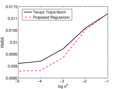
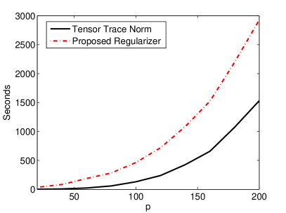
Figure 1: Synthetic dataset: (Left) Root Mean Squared Error (RMSE) of tensor trace norm and the proposed regularizer. (Right) Running time execution of both algorithms for different sizes of the tensor.

Furthermore, we have conducted an experiment to test the running time of both approaches. We have generated tensors $\boldsymbol{{\cal W}}^{0}\in\mathbb{R}^{p\times p\times p}$ for different values of $p\in\{20,\,40,\,\ldots,200\}$, following the same procedure as outlined above. The results are reported in Figure 1 (Right). For low values of $p$, the ratio between the running time of our approach and that of trace norm regularization is quite high. For example in the lowest value tried for $p$ in this experiment, $p=20$, this ratio is $22.661$. However, as the volume of the tensor increases, the ratio quickly decreases. For example, for $p=200$, the running time ratio is $1.9113$. These outcomes are expected since when $p$ is low, the most demanding routine in our method is the one described in Algorithm 1, where each iteration is of order $O\left(p\right)$ and $O\left(p^{2}\right)$ in the best and worst case, respectively. However, as $p$ increases the singular value decomposition routine, which is common to both methods, becomes the most demanding because it has a time complexity $O\left(p^{3}\right)$ [10]. Therefore, we can conclude that even though our approach is slower than the trace norm based method, this difference becomes much smaller as the size of the tensor increases.

5.2 School Dataset

The first real dataset we have tried is the Inner London Education Authority (ILEA) dataset . It is composed of examination marks ranging from $0$ to $70$, of $15362$ students which are described by a set of attributes such as school and ethnic group. Most of these attributes are categorical, thereby we can think of exam mark prediction as a tensor completion problem where each of the modes corresponds to a categorical attribute. In particular, we have used the following attributes: school ($139$), gender ($2$), VR-band ($3$), ethnic ($11$), and year ($3$), leading to a $5$-order tensor $\boldsymbol{{\cal W}}\in\mathbb{R}^{139\times 2\times 3\times 11\times 3}$.

We have selected randomly $5\%$ of the instances to make the test set and another $5\%$ of the instances for the validation set. From the remaining instances, we have randomly chosen $m$ of them for several values of $m$. This procedure has been repeated $20$ times and the average performance is presented in Figure 2 (Left). There is a distinguishable improvement of our approach with respect to tensor trace norm regularization. To check whether this gap is significant, we have conducted a set of paired $t$-tests for each value of $m$. In all cases we obtained a $p$-value below $0.01$.

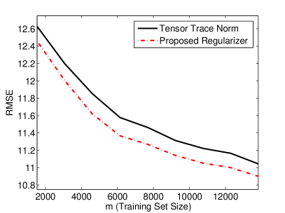
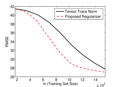
Figure 2: Root Mean Squared Error of tensor trace norm and the proposed regularizer for ILEA dataset (Left) and Ocean video (Right).

5.3 Video Completion

In the second real-data experiment we have performed a video completion test. Any video can be treated as a $4$-order tensor: “width” $\times$ “height” $\times$ “RGB” $\times$ “video length”, so we can use tensor completion algorithms to rebuild a video from a few inputs, a procedure that can be useful for compression purposes. In our case, we have used the Ocean video, available at [17]. This video sequence can be treated as a tensor $\boldsymbol{{\cal W}}\in\mathbb{R}^{160\times 112\times 3\times 32}$. We have randomly sampled $m$ tensors elements as training data, $5\%$ of them as validation data, and the remaining ones composed the test set. After repeating this procedure $10$ times, we present the average results in Figure 2 (Right). The proposed approach is noticeably better than the tensor trace norm in this experiment. This apparent outcome is strongly supported by the paired $t$-tests which we run for each value of $m$, obtaining always $p$-values below $0.01$, and for the cases $m>5\times 10^{4}$, we obtained $p$-values below $10^{-6}$.

6 Conclusion

In this paper, we proposed a convex relaxation for the average of the rank of the matricizations of a tensor. We compared this relaxation to a commonly used convex relaxation used in the context of tensor completion, which is based on the trace norm. We proved that this second relaxation is not tight and argued that the proposed convex regularizer may be advantageous. Empirical comparisons indicate that our method consistently improves in terms of estimation error over tensor trace norm regularization, while being computationally comparable on the range of problems we considered. In the future it would be interesting to study methods to speed up the computation of the proximity operator of our regularizer and investigate its utility in tensor learning problem beyond tensor completion such as multilinear multitask learning [20].

Appendix

In this appendix, we describe an auxiliary result and present the main steps for the computation of an approximate projection.

Appendix A A Useful Lemma

Lemma 4.

Let ${\cal C}_{1},\dots,{\cal C}_{N}$ be convex subsets of a Euclidean space and let ${\cal D}=\bigcap_{n=1}^{N}{\cal C}_{n}\neq\emptyset$. Let $g:\prod_{n=1}^{N}{\cal C}_{n}\rightarrow{\mathbb{R}}$ and let $h:{\cal D}\rightarrow{\mathbb{R}}$ be the function defined, for every $x\in{\cal D}$, as $h(x)=g(x,\dots,x)$. Then, for every $x\in{\cal D}$, it holds that

$$h^{**}(x)\geq g^{**}(x_{1},\dots,x_{N})\left|{}_{x_{n}=x,~{}\forall n\in[N]}\right..$$

Proof.

Since the restriction of $g$ on ${\cal D}^{N}\subseteq\prod_{n=1}^{N}{\cal C}_{n}$ equals to $h$, the convex envelope of $g$ when evaluated on the smaller set ${\cal D}^{N}$ cannot be larger than the convex envelope of $h$ on ${\cal D}$. ∎

Using this result it is immediately possible to derive a convex lower bound for the function $R$ in equation (2). Since the convex envelope of the rank function on the unit ball of the spectral norm is the trace norm, using Lemma 4 with ${\cal C}_{n}=\{{\boldsymbol{\cal W}}:\|W_{(n)}\|_{\infty}\leq 1\}$ and

$$g({\boldsymbol{\cal W}}_{1},\dots,{\boldsymbol{\cal W}}_{N})=\frac{1}{N}\sum_{n=1}^{N}{\rm rank}((W_{n})_{(n)}),$$

we conclude that the convex envelope of the function $R$ on the set ${\cal G}_{{\rm\infty}}$ is bounded from below by $\frac{1}{N}\sum_{n=1}^{N}\|W_{(n)}\|_{\rm tr}$. Likewise the convex envelope of $R$ on the set $\alpha{\cal G}_{{\rm 2}}$ is lower bounded by the function $\Omega_{\alpha}$ in equation (6).

Appendix B Computation of an Approximated Projection

Here, we address the issue of computing an approximate Euclidean projection onto the set

$$\mathcal{S}=\{v\in{\mathbb{R}}^{d}:v_{1}\geq\cdots\geq v_{d}\geq 0\}.$$

That is, for every $v$, we shall find a point ${\tilde{P}}_{\mathcal{S}}(v)\in{\cal S}$ such that

$$\left\|{\tilde{P}}_{\mathcal{S}}\left(v\right)-z\right\|_{2}\leq\left\|v-z\right\|_{2},\,\forall z\in\mathcal{S}.$$ (17)

As noted in [6], in order to build ${\tilde{P}}_{\mathcal{S}}$ such that this property holds true, it is useful to express the set of interest as the smallest one in a series of nested sets. In our problem, we can express $\mathcal{S}$ as

$\mathcal{S}=\mathcal{S}_{d}\subseteq\mathcal{S}_{d-1}\subseteq\ldots\subseteq\mathcal{S}_{1}$,

where $\mathcal{S}_{i}:=\left\{v\in\mathbb{R}^{d}\,:\,v_{1}\geq v_{2}\geq\ldots\geq v_{i},v\geq 0\right\}$. This property allows us to sequentially compute an approximate projection on the set ${\cal S}$ using the formula

$${\tilde{P}}_{\mathcal{S}}\left(v\right)=P_{\mathcal{S}_{d}}\left(P_{\mathcal{S}_{d-1}}\cdots\left(P_{\mathcal{S}_{1}}\left(v\right)\right)\right)$$ (18)

where, for every close convex set ${\cal C}$, we let $P_{\cal C}$ be the associated projection operator. Indeed, following [6], we can argue by induction on $i$ that ${\tilde{P}}_{\mathcal{S}}\left(v\right)$ verifies condition (17). The base case is $\left\|P_{\mathcal{S}_{1}}\left(v\right)-z\right\|_{2}=\left\|v-z\right\|_{2}$, which is obvious. Now, if for a given $1\leq i\leq d-1$ it holds that

$\left\|P_{\mathcal{S}_{i}}\left(\cdots P_{\mathcal{S}_{1}}\left(v\right)\right)-z\right\|_{2}\leq\left\|v-z\right\|_{2}$

then

$\left\|P_{\mathcal{S}_{i+1}}\left(P_{\mathcal{S}_{i}}\left(\cdots P_{\mathcal{S}_{1}}\left(v\right)\right)\right)-z\right\|_{2}\leq\left\|P_{\mathcal{S}_{i}}\left(\cdots P_{\mathcal{S}_{1}}\left(v\right)\right)-z\right\|_{2}\leq\left\|v-z\right\|_{2}$,

since $z$ is also contained in $\mathcal{S}_{i+1}$.

Note that to evaluate the right hand side of equation (18) we do not require full knowledge of $P_{{\cal S}_{i}}$, we only need to compute $P_{\mathcal{S}_{i+1}}(v)$ for $v\in\mathcal{S}_{i}$. The next proposition describes a recursive formula to achieve this step.

Proposition 5.

For any $v\in\mathcal{S}_{i}$, we express its first $i$ elements as $v_{1:i}=\left[v_{1:i-j},\,v_{i}\boldsymbol{1}^{j}\right]$, where the last $j\in[i]$ is the largest integer such that $v_{i-j+1}=v_{i-j+2}=\cdots=v_{i}$. It holds that

$$P_{\mathcal{S}_{i+1}}\left(v\right)=\begin{cases}v&{\rm if}\,v_{i}\geq v_{i+1}\\ \left[v_{1:i-j},\,\left(v_{i}+\frac{v_{i+1}-v_{i}}{j+1}\right)\boldsymbol{1}^{j+1},\,v_{i+2:d}\right]&{\rm if}\,v_{i}<v_{i+1}~{}{\rm and}~{}v_{i-j}\geq v_{i}+\frac{v_{i+1}-v_{i}}{j+1}\\ P_{\mathcal{S}_{i+1}}\left(\left[v_{1:i-j},\,v_{i-j}\boldsymbol{1}^{j},\,v_{i+1}-\left(v_{i-j}-v_{i}\right)j,\,v_{i+2:d}\right]\right)&{\rm otherwise},\end{cases}$$

where $\boldsymbol{1}^{d}\in\mathbb{R}^{d}$ denotes the vector containing $1$ in all its elements.

Proof.

The first case is straightforward. In the following we prove the remaining two. In both cases it will be useful to recall that the projection operator $P_{\mathcal{C}}$ on any convex set $\mathcal{C}$ is characterized as

$$x=P_{\mathcal{C}}\left(y\right)\Longleftrightarrow\left\langle y-x,\,z-x\right\rangle\leq 0,~{}\forall z\in\mathcal{C}.$$ (19)

  Input: $y\in\mathbb{R}_{+}^{d}$.

  Output: $v\in\mathcal{S}$.

  Initialization: $v\leftarrow y$.

  for $i=1,2,\dots,d$ do

     while $v_{i}<v_{i+1}$ do

        $j\leftarrow$ ${\rm argmax}\{\ell:\ell\in[i],v_{i}=v_{i-\ell+1}\}$

        if $v_{i}+\frac{v_{i+1}-v_{i}}{j+1}$ then

           $v_{1:i+1}\leftarrow\left[v_{1:i-j},\,\left(v_{i}+\frac{v_{i+1}-v_{i}}{j+1}\right)\boldsymbol{1}^{j+1}\right]$

        else

           $v_{1:i+1}\leftarrow\left[v_{1:i-j},\,v_{i-j}\boldsymbol{1}^{j},\,v_{i+1}-\left(v_{i-j}-v_{i}\right)j\right]$

        end if

     end while

  end for

Algorithm 2 Computing an approximated projection onto the set $\mathcal{S}=\{v\in{\mathbb{R}}^{d}:v_{1}\geq\cdots\geq v_{d}\geq 0\}$.

To prove the second case, we use property (19) and apply simple algebraic transformations to obtain, for all $z\in\mathcal{S}_{i+1}$, that

$$\left\langle v-P_{\mathcal{S}_{i+1}}\left(v\right),\,z-P_{\mathcal{S}_{i+1}}\left(v\right)\right\rangle=\frac{v_{i+1}-v_{i}}{j+1}\left(jz_{i+1}-\left\|z_{i-j+1:i}\right\|_{1}\right)\leq 0.$$

Finally we prove the third case. We want to show that if $x=P_{\mathcal{S}_{i+1}}(v)$ then

$$x=P_{\mathcal{S}_{i+1}}\left(\left[v_{1:i-j},\,v_{i-j}\boldsymbol{1}^{j},\,v_{i+1}-\left(v_{i-j}-v_{i}\right)j,\,v_{i+2:d}\right]\right).$$

By using property (19), the last equation is equivalent to the statement that if

$$\left\langle v-x,\,z-x\right\rangle\leq 0,\,\,\forall z\in\mathcal{S}_{i+1}~{}~{}{\rm then}$$ (20)

$$\left\langle\left[v_{1:i-j},\,v_{i-j}\boldsymbol{1}^{j},\,v_{i+1}-\left(v_{i-j}-v_{i}\right)j,\,v_{i+2:d}\right]-x,\,z-x\right\rangle\leq 0,\,\,\forall z\in\mathcal{S}_{i+1}.$$ (21)

A way to show that it holds true is to prove that the term in the left hand side of (21) is upper bounded by the corresponding term in (20). That is, for every $z\in\mathcal{S}_{i+1}$, we want to show that

$$\left\langle\left[v_{1:i-j},\,v_{i-j}\boldsymbol{1}^{j},\,v_{i+1}-\left(v_{i-j}-v_{i}\right)j,\,v_{i+2:d}\right]-v,z-x\right\rangle\leq 0.$$

A direct computation yields the equivalent inequality

$$\left(v_{i-j}-v_{i}\right)\left(jx_{i+1}-\left\|x_{i-j+1:i}\right\|_{1}+\left\|z_{i-j+1:i}\right\|_{1}-jz_{i+1}\right)\leq 0.$$ (22)

Since $x=P_{\mathcal{S}_{i+1}}\left(v\right)$, $v_{i-j+1}=v_{i-j+2}=\cdots=v_{i}$ and $v_{i+1}>v_{i}$, then $x_{i-j+1}=x_{i-j+2}=\cdots=x_{i+1}$. Consequently, the left hand side of inequality (22) is equivalent to

$$\left(v_{i-j}-v_{i}\right)\left(\left\|z_{i-j+1:i}\right\|_{1}-jz_{i+1}\right)\leq 0.$$

Note that the first factor is negative and the second is positive because $z$ and $v$ are in $\mathcal{S}_{i+1}$. The result follows. ∎

Algorithm 2 summarizes our method to compute the approximated projection operator onto the set $\mathcal{S}$, based on Proposition 5.

References

• [1]
• [2] A. Argyriou, C.A. Micchelli, M. Pontil, L. Shen and Y. Xu. Efficient first order methods for linear composite regularizers. arXiv:1104.1436, 2011.
• [3] R. Bhatia. Matrix Analysis. Springer Verlag, 1997.
• [4] D.P. Bertsekas, J.N. Tsitsiklis. Parallel and Distributed Computation: Numerical Methods. Prentice-Hall, 1989.
• [5] S. Boyd, N. Parikh, E. Chu, B. Peleato, and J. Eckstein. Distributed optimization and statistical learning via the alternating direction method of multipliers. Foundations and Trends in Machine Learning, 3(1):1–122, 2011.
• [6] S. Boyd, L. Xiao, A. Mutapcic. Subgradient methods, Stanford University, 2003.
• [7] P. L. Combettes and J.-C. Pesquet. Proximal splitting methods in signal processing. In Fixed-Point Algorithms for Inverse Problems in Science and Engineering (H. H. Bauschke et al. Eds), pages 185–212, Springer, 2011.
• [8] M. Fazel, H. Hindi, and S. Boyd. A rank minimization heuristic with application to minimum order system approximation. Proc. American Control Conference, Vol. 6, pages 4734–4739, 2001.
• [9] S. Gandy, B. Recht, I. Yamada. Tensor completion and low-n-rank tensor recovery via convex optimization. Inverse Problems, 27(2), 2011.
• [10] G. H. Golub, C. F. Van Loan. Matrix Computations. 3rd Edition. Johns Hopkins University Press, 1996.
• [11] Z. Harchaoui, M. Douze, M. Paulin, M. Dudik, J. Malick. Large-scale image classification with trace-norm regularization. IEEE Conference on Computer Vision & Pattern Recognition (CVPR), pages 3386–3393, 2012.
• [12] J-B. Hiriart-Urruty and C. Lemaréchal. Convex Analysis and Minimization Algorithms, Part I. Springer, 1996.
• [13] J-B. Hiriart-Urruty and C. Lemaréchal. Convex Analysis and Minimization Algorithms, Part II. Springer, 1993.
• [14] R.A. Horn and C.R. Johnson. Topics in Matrix Analysis. Cambridge University Press, 2005.
• [15] A. Karatzoglou, X. Amatriain, L. Baltrunas, N. Oliver. Multiverse recommendation: n-dimensional tensor factorization for context-aware collaborative filtering. Proc. 4th ACM Conference on Recommender Systems, pages 79–86, 2010.
• [16] T.G. Kolda and B.W. Bade. Tensor decompositions and applications. SIAM Review, 51(3):455–500, 2009.
• [17] J. Liu, P. Musialski, P. Wonka, J. Ye. Tensor completion for estimating missing values in visual data. Proc. 12th International Conference on Computer Vision (ICCV), pages 2114–2121, 2009.
• [18] Y. Nesterov. Gradient methods for minimizing composite objective functions. ECORE Discussion Paper, 2007/96, 2007.
• [19] B. Recht. A simpler approach to matrix completion. Journal of Machine Learning Research, 12:3413–3430, 2009.
• [20] B. Romera-Paredes, H. Aung, N. Bianchi-Berthouze and M. Pontil. Multilinear multitask learning. Proc. 30th International Conference on Machine Learning (ICML), pages 1444–1452, 2013.
• [21] N. Z. Shor. Minimization Methods for Non-differentiable Functions. Springer, 1985.
• [22] M. Signoretto, Q. Tran Dinh, L. De Lathauwer, J.A.K. Suykens. Learning with tensors: a framework based on convex optimization and spectral regularization. Machine Learning, to appear.
• [23] M. Signoretto, R. Van de Plas, B. De Moor, J.A.K. Suykens. Tensor versus matrix completion: a comparison with application to spectral data. IEEE Signal Processing Letters, 18(7):403–406, 2011.
• [24] N. Srebro, J. Rennie and T. Jaakkola. Maximum margin matrix factorization. Advances in Neural Information Processing Systems (NIPS) 17, pages 1329–1336, 2005.
• [25] R. Tomioka, K. Hayashi, H. Kashima, J.S.T. Presto. Estimation of low-rank tensors via convex optimization. arXiv:1010.0789, 2010.
• [26] R. Tomioka and T. Suzuki. Convex tensor decomposition via structured Schatten norm regularization. arXiv:1303.6370, 2013.
• [27] R. Tomioka, T. Suzuki, K. Hayashi, H. Kashima. Statistical performance of convex tensor decomposition. Advances in Neural Information Processing Systems (NIPS) 24, pages 972–980, 2013.