Ginzburg-Landau vortices, Coulomb Gases, and Renormalized Energies

Abstract

This is a review about a series of results on vortices in the Ginzburg-Landau model of superconductivity on the one hand, and point patterns in Coulomb gases on the other hand, as well as the connections between the two topics.

keywords: Ginzburg-Landau equations, superconductivity, vortices, Coulomb Gas, one-component plasma, jellium, Renormalized energy.

Most of this paper describes joint work with Etienne Sandier, which has naturally led from the study of the Ginzburg-Landau equations of superconductivity – a rather involved system of PDE – to that of a well-known statistical mechanics system: namely the classical Coulomb gas. We will review results in each area and explain the similarity in the mathematics involved.

1 The Ginzburg-Landau model of superconductivity

A type-II superconductor, cooled down below its critical temperature experiences the circulation of “superconducting currents” without resistance, and has a particular response in the presence of an applied magnetic field. Above a certain value of the external field called the first critical field, vortices appear. When the field is large enough, the experiments (dating from the 60’s) show that they arrange themselves in (often) perfect triangular lattices, cf. http://www.fys.uio.no/super/vortex/ or Fig. 1 below.

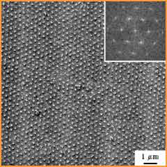
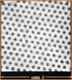
Figure 1: Abrikosov lattices

These are named Abrikosov lattices after the physicist Abrikosov who had predicted, from the Ginzburg-Landau model, that periodic arrays of vortices should appear [A]. These vortices repel each other like Coulomb charges would, while being confined inside the sample by the applied magnetic field. Their triangular lattice arrangement is the result of these two opposing effects.

1.1 The model

The Ginzburg-Landau model was introduced on phenomenological grounds by Landau and Ginzburg in the 50’s [GL] ; after some nondimensionalizing procedure, in a two-dimensional domain $\Omega$ it takes the form

(1) $$GL_{\varepsilon}(\psi,A)=\frac{1}{2}\int_{\Omega}|(\nabla-iA)\psi|^{2}+|\nabla\times A-h_{ex}|^{2}+\frac{1}{2\varepsilon^{2}}\left(1-|\psi|^{2}\right)^{2}$$

Here $\psi$ is a complex-valued function, called “order parameter” and indicating the local state of the sample: $|\psi|^{2}$ is the density of “Cooper pairs” of superconducting electrons. With our normalization $|\psi|\leq 1$, and where $|\psi|\simeq 1$ the material is in the superconducting phase, while where $|\psi|=0$, it is in the normal phase (i.e. behaves like a normal conductor), the two phases being able to coexist in the sample.

The vector field $A$ is the gauge field or vector potential of the magnetic field. The magnetic field in the sample is deduced by $h=\nabla\times A={\rm curl\,}A=\partial_{1}A_{2}-\partial_{2}A_{1}$, it is thus a real-valued function in $\Omega$.

Finally, the parameter $\varepsilon$ is a material constant, it is the inverse of the “Ginzburg-Landau parameter” usually denoted $\kappa$. It is also the ratio between the “coherence length” usually denoted $\xi$ (roughly the vortex-core size) and the “penetration length” of the magnetic field usually denoted $\lambda$. We are interested in the regime of small $\varepsilon$, corresponding to high-$\kappa$ (or extreme type-II) superconductors. The limit $\varepsilon\to 0$ or $\kappa\to\infty$ that we will consider is also called the London limit.

This is a $\mathbb{U}(1)$-gauge theory and the functional (as well as all the physically meaningful quantities) is invariant under the gauge-change

(2) $$\left\{\begin{array}[]{ll}\psi\mapsto\psi e^{i\Phi}\\ A\mapsto A+\nabla\Phi\end{array}\right.$$

where $\Phi$ is a smooth enough function.

The stationary states of the system are the critical points of $GL_{\varepsilon}$, or the solutions of the Ginzburg-Landau equations :

$(\mathrm{GL})\{$ $$\begin{aligned} -(\nabla_{A})^{2}\psi=\frac{1}{\varepsilon^{2}}\psi(1-|\psi|^{2})&\quad\text{in $\Omega$}\\ -\nabla^{\perp}h=\langle i\psi,\nabla_{A}\psi\rangle&\quad\text{in $\Omega$}\\ h={h_{\rm ex}}&\quad\text{on $\partial\Omega$}\\ \nabla_{A}\psi\cdot\nu=0&\quad\text{on $\partial\Omega$,}\\ \end{aligned}\right.$$

where $\nabla^{\perp}$ denotes the operator $(-\partial_{2},\partial_{1})$, $\nabla_{A}=\nabla-iA$, and $\nu$ is the outer unit normal to $\partial\Omega$. Here appears the superconducting current, a real valued vector field given by $j=\langle i\psi,\nabla_{A}\psi\rangle$ where $\langle.,.\rangle$ denotes the scalar-product in $\mathbb{C}$ identified with $\mathbb{R}^{2}$. It may also be written as

$$\frac{i}{2}\left(\psi\overline{\nabla_{A}\psi}-\bar{\psi}\nabla_{A}\psi\right),$$

where the bar denotes the complex conjugation. For further details on the model, we refer to [GL, DeG, T, FH, SS1].

The Ginzburg-Landau model has led to a large amount of theoretical physics literature — probably most relevant to us is the book by De Gennes [DeG]. However, a precise mathematical proof of the phase transition at the first critical field, and of the emergence of the Abrikosov lattice as the ground state for the arrangement of the vortices was still missing.

In the 90’s, researchers coming from nonlinear analysis and PDEs became interested in the model (precursors were Berger, Rubinstein, Schatzman, Chapman, Du, Baumann, Phillips… cf. e.g. [Ch, DGP] for reviews), with the notable contribution of Bethuel-Brezis-Hélein [BBH] who introduced systematic tools and asymptotic estimates to study vortices, but in the simplified Ginzburg-Landau equation not containing the magnetic gauge, and allowing only for a fixed number of vortices. This was then adapted to the model with gauge but with a different boundary condition by Bethuel and Rivière [BR1, BR2]. It was however not clear that this approach could work to treat the case of the full magnetic model when the number of vortices gets unbounded as $\varepsilon\to 0$. It is only with the works of Sandier [Sa] and Jerrard [Je] that tools capable of handling this started to be developed. Relying on these tools and expanding them, in a series of works later revisited in a book [SS1], we analyzed the full model and obtained the proof of the phase transition, and the computation of the asymptotics of the first critical field in the limit $\varepsilon\to 0$. We characterized the optimal number and distribution of the vortices and derived in particular a “mean-field regime” limiting distribution for the vortices, which will be described just below. Note that this analysis and the tools developed to understand the vortices have proven useful to study vortices in rotating superfluids like Bose-Einstein condensates (cf. e.g. [CPRY] and references therein), a problem which has a large similarity with Ginzburg-Landau from the mathematical perspective, and of current interest for experiments.

1.2 Critical fields and vortices

What are vortices? A vortex is an object centered at an isolated zero of $\psi$, around which the phase of $\psi$ has a nonzero winding number, called the degree of the vortex. So it is also a small defect of normal phase in the superconducting phase, surrounded by a loop of superconducting current. When $\varepsilon$ is small, it is clear from (1) that any discrepancy between $|\psi|$ and $1$ is strongly penalized, and a scaling argument hints that $|\psi|$ is different from $1$ only in regions of characteristic size $\varepsilon$. A typical vortex centered at a point $x_{0}$ behaves like $\psi=\rho e^{i\,\varphi}$ with $\rho=f(\frac{|x-x_{0}|}{\varepsilon})$ where $f(0)=0$ and $f$ tends to $1$ as $r\to+\infty$, i.e. its characteristic core size is $\varepsilon$, and

$$\frac{1}{2\pi}\int_{\partial B(x_{0},R\varepsilon)}\frac{\partial\varphi}{\partial\tau}=d\in\mathbb{Z}$$

is an integer, called the degree of the vortex. For example $\varphi=d\theta$ where $\theta$ is the polar angle centered at $x_{0}$ yields a vortex of degree $d$ at $x_{0}$.

There are three main critical values of ${h_{\rm ex}}$ or critical fields ${H_{c_{1}}}$, ${H_{c_{2}}}$, and ${H_{c_{3}}}$, for which phase-transitions occur.

• For ${h_{\rm ex}}<{H_{c_{1}}}$ there are no vortices and the energy minimizer is the superconducting state $(\psi\equiv 1,A\equiv 0)$. (This is a true solution if ${h_{\rm ex}}=0$, and a solution close to this one (i.e. with $|\psi|\simeq 1$ everywhere) persists if ${h_{\rm ex}}$ is not too large.) It is said that the superconductor “expels” the applied magnetic field, this is the “Meissner effect”, and the corresponding solution is called the Meissner solution.

• For ${h_{\rm ex}}={H_{c_{1}}}$, which is of the order of ${|\mathrm{log}\ \varepsilon|}$ as $\varepsilon\to 0$, the first vortice(s) appear.

• For ${H_{c_{1}}}<{h_{\rm ex}}<{H_{c_{2}}}$ the superconductor is in the “mixed phase” i.e. there are vortices, surrounded by superconducting phase where $|\psi|\simeq 1$. The higher ${h_{\rm ex}}>{H_{c_{1}}}$, the more vortices there are. The vortices repel each other so they tend to arrange in these triangular Abrikosov lattices in order to minimize their repulsion.

• For ${h_{\rm ex}}={H_{c_{2}}}\sim\frac{1}{\varepsilon^{2}}$, the vortices are so densely packed that they overlap each other, and a second phase transition occurs, after which $|\psi|\sim 0$ inside the sample, i.e. all superconductivity in the bulk of the sample is lost.

• For ${H_{c_{2}}}<{h_{\rm ex}}<{H_{c_{3}}}$ superconductivity persists only near the boundary, this is called surface superconductivity. More details and the mathematical study of this transition are found in [FH] and references therein.

• For ${h_{\rm ex}}>{H_{c_{3}}}=O(\frac{1}{\varepsilon^{2}})$ (defined in decreasing fields), the sample is completely in the normal phase, corresponding to the “normal” solution $\psi\equiv 0,h\equiv{h_{\rm ex}}$ of (GL). See [GP] for a proof.

1.3 Formal correspondence

Given a family of configurations $(\psi_{\varepsilon},A_{\varepsilon})$ it turns out to be convenient to express the energy in terms of the induced magnetic field $h_{\varepsilon}(x)=\nabla\times A_{\varepsilon}(x)$. Taking the curl of the second relation in (GL) we obtain

$$-\Delta h_{\varepsilon}+h_{\varepsilon}={\rm curl\,}\langle i\psi_{\varepsilon},\nabla_{A_{\varepsilon}}\psi_{\varepsilon}\rangle+h_{\varepsilon}\simeq{\rm curl\,}\nabla\varphi_{\varepsilon}$$

where we approximate $|\psi_{\varepsilon}|$ by $1$ and where $\varphi_{\varepsilon}$ denotes the phase of $\psi_{\varepsilon}$. One formally has that ${\rm curl\,}\nabla\varphi_{\varepsilon}=2\pi\sum_{i}d_{i}\delta_{a_{i}}$ where $\{a_{i}\}_{i}$ is the collection of zeroes of $\psi$, i.e. the vortex centers (really depending on $\varepsilon$), and $d_{i}\in\mathbb{Z}$ are their topological degrees. This is not exact, however it can be given some rigorous meaning in the asymptotics $\varepsilon\to 0$. We may rewrite this equation in a more correct manner

(3) $$\left\{\begin{array}[]{ll}-\Delta h_{\varepsilon}+h_{\varepsilon}\simeq 2\pi\sum_{i}d_{i}\delta_{a_{i}}^{(\varepsilon)}&\text{in}\ \Omega\\ h={h_{\rm ex}}&\text{on}\ \partial\Omega,\end{array}\right.$$

where the exact right-hand side in (3) is a sum of quantized charges, or Dirac masses, which should be thought of as somehow smeared out at a scale of order $\varepsilon$. This relation is called in the physics literature the London equation (it is usually written with true Dirac masses, but this only holds approximately). It indicates how the magnetic field penetrates in the sample through the vortices.

Some computations (with the help of all the mathematical machinery developed to describe vortices) lead eventually to the conclusion that everything happens as if the Ginzburg-Landau energy $GL_{\varepsilon}$ of a configuration were equal to

(4) $$GL_{\varepsilon}(\psi_{\varepsilon},A_{\varepsilon})\simeq\frac{1}{2}\int_{\Omega}|\nabla h_{\varepsilon}|^{2}+|h_{\varepsilon}-{h_{\rm ex}}|^{2}\\ =\frac{1}{2}\iint_{\Omega\times\Omega}G_{\Omega}(x,y)\Big{(}2\pi\sum_{i}d_{i}\delta_{a_{i}}^{(\varepsilon)}-{h_{\rm ex}}\Big{)}(x)\Big{(}2\pi\sum_{i}d_{i}\delta_{a_{i}}^{(\varepsilon)}-{h_{\rm ex}}\Big{)}(y),$$

where $G_{\Omega}$ is a type of Green kernel, solution to

(5) $$\begin{cases}-\Delta G_{\Omega}+G_{\Omega}=\delta_{y}&\text{in }\ \Omega\\ G_{\Omega}=0&\text{on}\ \partial\Omega,\end{cases}$$

and $h_{\varepsilon}$ solves (3). With this way of writing, and in view of the logarithmic nature of $G_{\Omega}$, one recognizes essentially a pairwise Coulomb interaction of positive charges in a constant negative background ($-{h_{\rm ex}}$), which is what leads to the analogy with the Coulomb gas described later. There remains to understand for which value of ${h_{\rm ex}}$ vortices become favorable, and with which distribution. To really understand that, the effect of the “smearing out” of the Dirac charges needs to be more carefully accounted for. Instead of each vortex having any infinite cost in (4) (which would be the case with true Diracs) the real cost of each vortex can be evaluated as being $\sim\pi d_{i}^{2}{|\mathrm{log}\ \varepsilon|}$ per vortex (roughly the equivalent of the cost generated by a Dirac mass smeared out at the scale $\varepsilon$). We may thus evaluate (4) as

(6) $$\frac{GL_{\varepsilon}(\psi_{\varepsilon},A_{\varepsilon})}{{h_{\rm ex}}^{2}}\simeq\frac{{|\mathrm{log}\ \varepsilon|}}{{h_{\rm ex}}}\frac{\pi\sum_{i}d_{i}^{2}}{{h_{\rm ex}}}+\frac{{h_{\rm ex}}^{2}}{2}\int_{\Omega}|\nabla h|^{2}+|h-1|^{2}$$

where $h=\lim_{\varepsilon\to 0}\frac{h_{\varepsilon}}{{h_{\rm ex}}}$.

Optimizing over the degrees $d_{i}$’s allows to see that the degrees $d_{i}=1$ are the only favorable ones. In view of (3), assuming this is true we can then rewrite $\pi\sum_{i}d_{i}^{2}$ as $\frac{1}{2}\int_{\Omega}|-\Delta h_{\varepsilon}+h_{\varepsilon}|$. Passing to the limit $\varepsilon\to 0$, and assuming $\frac{{h_{\rm ex}}}{{|\mathrm{log}\ \varepsilon|}}\to\lambda$ as $\varepsilon\to 0$, we find that the mean-field limit energy arising from (4) is

(7) $$\frac{GL_{\varepsilon}}{{h_{\rm ex}}^{2}}\simeq_{\varepsilon\to 0}\mathcal{E}^{MF}_{\lambda}(h)=\frac{1}{2\lambda}\int_{\Omega}|-\Delta h+h|+\frac{1}{2}\int_{\Omega}|\nabla h|^{2}+|h-1|^{2}\\ =\frac{1}{2\lambda}\int_{\Omega}|\mu|+\frac{1}{2}\iint_{\Omega\times\Omega}G_{\Omega}(x,y)d(\mu-1)(x)\,d(\mu-1)(y)$$

where $h$ is here related to the limiting “vorticity” (or vortex density) $\mu:=\lim_{\varepsilon\to 0}\frac{1}{{h_{\rm ex}}}2\pi\sum_{i}d_{i}\delta_{a_{i}}$ by $-\Delta h+h=\mu$ in $\Omega$ with $h=1$ on $\partial\Omega$, simply by taking the limit of (3).

In (7) the first contribution to the energy corresponds the total self-interaction of the vortices in (4), while the second one is the cross-interaction of the vortices and the vortices and the equivalent background charge (which is really the result of the confinement effect of the applied magnetic field).

We have the following rigorous statement.

Theorem 1 ([SS2], [SS1] Chap. 7).

Assume ${h_{\rm ex}}\sim\lambda{|\mathrm{log}\ \varepsilon|}$ as $\varepsilon\to 0$, where $\lambda>0$ is a constant independent of $\varepsilon$. If $(\psi_{\varepsilon},A_{\varepsilon})$ minimizes $GL_{\varepsilon}$, then as $\varepsilon\to 0$

$$\frac{2\pi\sum_{i}d_{i}\delta_{a_{i}}}{{h_{\rm ex}}}\to\mu_{*}\quad\text{in the weak sense of measures}$$

where $\mu_{*}$ is the unique minimizer of $\mathcal{E}^{MF}_{\lambda}$. Moreover

(8) $$\min GL_{\varepsilon}={h_{\rm ex}}^{2}(\min\mathcal{E}^{MF}_{\lambda}+o(1))\quad\text{as}\ \varepsilon\to 0.$$

Minimizing $\mathcal{E}^{MF}_{\lambda}$ leads to a standard variational problem called an “obstacle problem”. The corresponding optimal distribution of vorticity is uniform of density $1-1/(2\lambda)$ on a subdomain $\omega_{\lambda}$ of $\Omega$ depending only on $\lambda$.

An easy analysis of this obstacle problem yields the following (cf. also Fig. 2):

1. $\omega_{\lambda}=\varnothing$ (hence $\mu_{*}=0$) if and only if $\lambda<\lambda_{\Omega}$, where $\lambda_{\Omega}$ is given by

   (9) $$\lambda_{\Omega}=(2\max|h_{0}-1|)^{-1}$$

   for $h_{0}$ the solution to

   (10) $$\left\{\begin{array}[]{ll}-\Delta h_{0}+h_{0}=0&\text{in}\ \Omega\\ h_{0}=1&\text{on}\ \partial\Omega.\end{array}\right.$$

2. For $\lambda>\lambda_{\Omega}$, the measure of $\omega_{\lambda}$ is nonzero, so the limiting vortex density $\mu_{*}\neq 0$. Moreover, as $\lambda$ increases (i.e. as ${h_{\rm ex}}$ does), the set $\omega_{\lambda}$ increases. When $\lambda=+\infty$ (this corresponds to the case ${h_{\rm ex}}\gg{|\mathrm{log}\ \varepsilon|}$), $\omega_{\lambda}$ becomes $\Omega$ and $\mu_{*}=\mathbf{1}_{\Omega}$.

Figure 2: Optimal density of vortices according to the obstacle problem.

Since ${H_{c_{1}}}$ corresponds to the applied field for which minimizers start to have vortices, this leads us to expecting that

(11) $$\boxed{{H_{c_{1}}}\sim\lambda_{\Omega}{|\mathrm{log}\ \varepsilon|}\quad\text{as}\ \varepsilon\to 0}$$

where $\lambda_{\Omega}$ depends only on $\Omega$ via (9)–(10).

In fact this is true, because we were able to show that below this value ${H_{c_{1}}}$, not only the average vortex density $\mu_{*}$ is $0$, but there are really no vortices. To see this, a more refined asymptotic expansion of $GL_{\varepsilon}$ than (7) is needed. It suffices instead to note that in the regime when a zero or small number of vortices is expected, the solution to (3) is well approximated by ${h_{\rm ex}}h_{0}$ where $h_{0}$ solves (10), and then to split the true $h_{\varepsilon}$ as ${h_{\rm ex}}h_{0}+h_{1,\varepsilon}$ where $h_{1,\varepsilon}$ is a remainder term, and expand the energy $GL_{\varepsilon}$ in terms of this splitting.

Let us state the result we obtain when looking this way more carefully at the regime ${h_{\rm ex}}\sim\lambda_{\Omega}{|\mathrm{log}\ \varepsilon|}$ and analyzing individual vortices. For simplicity, we assume that the function $h_{0}$ achieves a unique minimum at a point $p\in\Omega$ (this is satisfied for example if $\Omega$ is convex) and that its Hessian at that point, $Q$, is nondegenerate.

Theorem 2 ([Se1, Se2], [SS1] Chap. 12).

There exists an increasing sequence of values

$$H_{n}=\lambda_{\Omega}{|\mathrm{log}\ \varepsilon|}+(n-1)\lambda_{\Omega}\log\frac{{|\mathrm{log}\ \varepsilon|}}{n}+\text{constant order terms}$$

such that if ${h_{\rm ex}}\leq\lambda_{\Omega}{|\mathrm{log}\ \varepsilon|}+O(\log\ {|\mathrm{log}\ \varepsilon|})$ and ${h_{\rm ex}}\in(H_{n},H_{n+1})$, then global minimizers of $GL_{\varepsilon}$ have exactly $n$ vortices of degree 1, at points $a_{i}^{\varepsilon}\to{p}$ as $\varepsilon\to 0$, and the $\tilde{a_{i}^{\varepsilon}}:=\sqrt{\frac{{h_{\rm ex}}}{n}}(a_{i}^{\varepsilon}-p)$ converge as $\varepsilon\to 0$ to a minimizer of

(12) $$w_{n}(x_{1},\cdots,x_{n})=-\sum_{i\neq j}\log|x_{i}-x_{j}|+n\sum_{i=1}^{n}Q(x_{i}).$$

We find here the precise value of ${H_{c_{1}}}$ for which the first vortex appears in the minimizers, and then a sequence of “critical fields” for which a second, a third, etc.. vortices appear in minimizers, together with a characterization of their optimal locations, governed by an explicit interaction energy $w_{n}$.

1.4 The next order study

Theorem 1 above proved that above ${H_{c_{1}}}$, for $\lambda>\lambda_{\Omega}$, the number of vortices is proportional to ${h_{\rm ex}}$ and they are uniformly distributed in a subregion of the domain, but it is still far from explaining the optimality of the Abrikosov lattice. To (begin to) explain it, one needs to look at the next order in the energy asymptotics (7), and at the blown-up of (3) at the inverse of the intervortex distance scale, which here is simply $\sqrt{{h_{\rm ex}}}$. For simplicity, let us reduce to the case $\lambda=1$ (or ${h_{\rm ex}}\gg{|\mathrm{log}\ \varepsilon|}$) where the limiting optimal measure is $\mu_{*}=\mathbf{1}_{\Omega}$ and the limiting $h\equiv 1$.

Once the blow-up by $\sqrt{{h_{\rm ex}}}$ is performed and the limit $\varepsilon\to 0$ is taken, (3) becomes

(13) $$-\Delta H+1=2\pi\sum_{a}\delta_{a}\quad\text{in}\ \mathbb{R}^{2}$$

where the limiting blown-up points $a$ form an infinite configuration in the plane, and these are now true Diracs (one may in fact reduce to the case where all degrees are equal to $+1$, other situations being energetically too costly).

One may recognize here essentially a jellium of infinite size, and $E=\nabla H$ the electric field generated by the points (its rotated vector field $j=-E^{\perp}$ corresponds to the superconducting current in superconductivity). The jellium model was first introduced by Wigner, and it means an infinite set of point charges with identical charges with Coulomb interaction, screened by a uniform neutralizing background, here the density $-1$. It is also called a one-component plasma.

It then remains first to identify and define a limiting interaction energy for this “jellium,” and second to derive it from $GL_{\varepsilon}$. The energy, that will be denoted $W$, arises as a next order correction term in the expansion of $\min GL_{\varepsilon}$ beyond the order ${h_{\rm ex}}^{2}$ term identified by (7)-(8).

Isolating efficiently the next order terms in $GL_{\varepsilon}$ relies on another “splitting” of the energy. Instead of expanding $h_{\varepsilon}$ near ${h_{\rm ex}}h_{0}$ as in the case with few vortices, one should expand around ${h_{\rm ex}}h_{\lambda}$ where $h_{\lambda}$ is the minimizer of $\mathcal{E}^{MF}_{\lambda}$, i.e. the solution to the obstacle problem above. Splitting $h_{\varepsilon}={h_{\rm ex}}h_{\lambda}+h_{1,\varepsilon}$ where $h_{1,\varepsilon}$ is seen as a remainder, turns out to exactly isolate the leading order contribution ${h_{\rm ex}}^{2}\min\mathcal{E}^{MF}_{\lambda}$ from an explicit lower order term.

1.4.1 The renormalized energy: definition and properties

We next turn to discussing the effective interaction energy between the blown-up points. As we said, it should be a total Coulomb interaction between the points (seen as discrete positive point charges) and the fixed constant negative background “charge”. Of course defining the total Coulomb interaction of such a system is delicate because several difficulties arise: first, the infinite number of charges and the lack of local charge neutrality, which lead us to defining the energy as a thermodynamic limit; second the need to remove the infinite self-interaction created by each point charge, now that we are dealing with true Diracs.

Let us now define the interaction energy $W$. Let $m>0$ be a given positive number (corresponding to the density of points). We say a vector field $E$ belongs to the class $\mathcal{A}_{m}$ if

(14) $$E=\nabla H\quad-\Delta H=2\pi(\nu-m)\quad\mbox{for some}\ \nu=\sum_{p\in\Lambda}\delta_{p},\quad\mbox{where }\ \Lambda\ \mbox{is a discrete set in \ }\mathbb{R}^{2}.$$

As said above, the vector-field $E$ physically corresponds, in the electrostatic analogy, to the electric field generated by the point charges, and $-E^{\perp}$ to a superconducting current in the superconductivity context.

Note that $H$ has a logarithmic singularity near each $a$, and thus $|\nabla H|^{2}$ is not integrable; however, when removing small balls of radius $\eta$ around each $a$, adding back $\pi\log\eta$, and letting $\eta\to 0$, this singularity can be “resolved”.

Definition 1.

We define the renormalized energy $W$ for $E\in\mathcal{A}_{m}$ by

(15) $$W(E):=\limsup_{R\to\infty}\frac{W(E,\chi_{B_{R}})}{|B_{R}|},$$

where $\chi_{B_{R}}$ is any cutoff function supported in $B_{R}$ with $\chi_{B_{R}}=1$ in $B_{R-1}$ and $|\nabla\chi_{B_{R}}|\leq C$, and $W(E,\chi)$ is defined by

(16) $$W(E,\chi):=\lim_{{\eta\to 0}}\int_{\mathbb{R}^{2}\setminus\cup_{i=1}^{n}B(x_{i},\eta)}{\chi}|E|^{2}+\pi{(\log\eta)}\sum_{i}{\chi}(x_{i}).$$

The name is given by analogy with the “renormalized energy” introduced in [BBH] as the effective interaction energy of a finite number of point vortices. Renormalized refers here to the way the energy is computed by substracting off the infinite contribution corresponding to the self interaction of each charge or vortex.

In the particular case where the configuration of points $\Lambda$ has some periodicity, i.e. if it can be seen as $n$ points $a_{1},\cdots,a_{n}$ living on a torus ${\mathbb{T}}$ of appropriate size, then $W$ can be expressed much more simply as a function of the points only:

(17) $$W(a_{1},\cdots,a_{n})=\frac{\pi}{|{\mathbb{T}}|}\sum_{j\neq k}G(a_{j}-a_{k})+\pi\lim_{x\to 0}\left(G(x)+\log|x|\right),$$

where $G$ is the Green’s function of the torus (i.e. solving $-\Delta G=\delta_{0}-1/|{\mathbb{T}}|$). The Green function of the torus can itself be expressed explicitely in terms of some Eisenstein series and the Dedekind Eta function. The definition (15) thus allows to generalize such a formula to any infinite system, without any periodicity assumption.

The question of central interest to us is that of understanding the minimum and minimizers of $W$. Here are a few remarks.

1. The value of $W$ doesn’t really depend on the cutoff functions satisfying the assumption.

2. $W$ is unchanged by a compact perturbation of the points.

3. One can reduce by scaling to studying $W$ over the class $\mathcal{A}_{1}$.

4. It can be proven that minimizers of $W$ over $\mathcal{A}_{1}$ exist (and the minimum is finite).

5. It can be proven that the minimum of $W$ is equal to the limit as $N\to\infty$ of the minimum of $W$ over configurations of points which are $N\times N$ periodic.

We do not know the value of $\min_{\mathcal{A}_{1}}W$, however we can identify the minimum of $W$ over a restricted class: that of points on a perfect lattice (of volume $1$).

Theorem 3 ([SS5]).

The minimum of $W$ over perfect lattice configurations (of density $1$) is achieved uniquely, modulo rotations, by the triangular lattice.

By triangular lattice, we mean the lattice $\mathbb{Z}+\mathbb{Z}e^{i\pi/3}$, properly scaled.

The proof of this theorem uses the explicit formula for $W$ in the periodic case in terms of Eisenstein series mentioned above. By transformations using modular functions or by direct computations, minimizing $W$ becomes equivalent to minimizing the Epstein zeta function $\zeta(s)=\sum_{p\in\Lambda}\frac{1}{|p|^{s}}$, $s>2$, over lattices. Results from number theory in the 60’s to 80’s (due to Cassels, Rankin, Ennola, Diananda, Montgomery, cf. [Mo] and references therein) say that this is minimized by the triangular lattice.

In view of the experiments showing Abrikosov lattices in superconductors, it is then natural to formulate the

Conjecture 1.

The “Abrikosov” triangular lattice is a global minimizer of $W$.

Observe that this question belongs to the more general family of crystallization problems. A typical such question is, given a potential $V$ in any dimension, to determine the point positions that minimize

$$\sum_{i\neq j}V(x_{i}-x_{j})$$

(with some kind of boundary condition), or rather

$$\lim_{R\to\infty}\frac{1}{|B_{R}|}\sum_{i\neq j,x_{i},x_{j}\in B_{R}}V(x_{i}-x_{j}),$$

and to determine whether the minimizing configurations are perfect lattices. Such questions are fundamental in order to understand the crystalline structure of matter. They also arise in the arrangement of Fekete points, “Smale’s problem” on the sphere, or the “Cohn-Kumar conjecture”… One should immediately stress that there are very few positive results in that direction in the literature (in fact it is very rare to have a proof that the solution to some minimization problem is periodic). Some exceptions include the two-dimensional sphere packing problem, for which Radin [Ra] showed that the minimizer is the triangular lattice, and an extension of this by Theil [Th] for a class of very short range Lennard-Jones potentials. Here the corresponding potential is rather logarithmic, hence long-range, and these techniques do not apply. The question could also be rephrased as that of finding

$$\min``\|\sum_{i}\delta_{x_{i}}-1\|_{(H^{1})^{*}}"$$

where the quantity is put between brackets to recall that $\delta_{x_{i}}$ does not really belong to the dual of the Sobolev space $H^{1}$ but rather has to be computed in the renormalized way that defines $W$. A closely related problem: to find

$$\min\|\sum_{i}\delta_{x_{i}}-1\|_{Lip^{*}}$$

turns out to be much easier. It is shown in [BPT] with a relatively short proof that again the triangular lattice achieves the minimum.

With S. Rota Nodari, in [RNS], we investigated further the structure of minimizers of $W$ (or rather, a suitable modification of it) and we were able to prove that the energy density and the points were uniformly distributed at any scale $\gg 1$, in good agreement with (but of course much weaker than!) the conjecture of periodicity of the minimizers.

Even though the minimization of $W$ is only conjectural, it is natural to view it as (or expect it to be) a quantitative “measure of disorder” of a configuration of points in the plane. In this spirit, in [BS] we use $W$ to quantify and compute explicitly the disorder of some classic random point configurations in the plane and on the real line.

1.4.2 Next order result for $GL_{\varepsilon}$

We can now state the main next order result on $GL_{\varepsilon}$.

Theorem 4 ([SS5]).

Consider minimizers $(\psi_{\varepsilon},A_{\varepsilon})$ of the Ginzburg-Landau in the regime $\lambda_{\Omega}{|\mathrm{log}\ \varepsilon|}\leq{h_{\rm ex}}\ll\frac{1}{\varepsilon^{2}}$. After blow-up at scale $\sqrt{{h_{\rm ex}}}$ around a randomly chosen point in $\omega_{\lambda}$, the $\nabla h_{\varepsilon}$ converge as $\varepsilon\to 0$ to vector fields in the plane which, almost surely, minimize $W$. Moreover, $\min GL_{\varepsilon}$ can be computed up to $o({h_{\rm ex}})$ (i.e. up to an error $o(1)$ per vortex):

$$\min GL_{\varepsilon}={h_{\rm ex}}^{2}\min\mathcal{E}^{MF}_{\lambda}+(1-\frac{1}{2\lambda}){h_{\rm ex}}|\omega_{\lambda}|\min_{\mathcal{A}_{1}}W+o({h_{\rm ex}})\quad\text{as}\ \varepsilon\to 0.$$

Thus, our study reduces the problem to understanding the minimization of $W$. If the last step of proving Conjecture 1 was accomplished, this would completely justify the emergence of the Abrikosov lattice in superconductors.

1.5 Other results

We also investigated the structure of solutions to (GL) which are not necessarily minimizing, in other words critical points of (1). Let us list here the main results:

• In [Se2] and [SS1, Chap 12], we prove the existence of branches of local minimizers of (1) (hence stable solutions) of similar type as the solutions in Theorem 2 which have arbitrary bounded numbers of vortices all of degree $+1$ and exist for wide ranges of the parameter ${h_{\rm ex}}$, and the locations of the vortices in these solutions are also characterized. In other words, for a given ${h_{\rm ex}}$, there may exist an infinite number of stable solutions with vortices, indexed by the number of vortices. Only one specific value of the number of vortices is optimal, depending on the value of ${h_{\rm ex}}$, as in Theorem 2.

• Similarly, there also exist multiple branches of locally minimizing solutions of (GL) with (rather arbitrary) unbounded numbers of vortices. This is proven in [CS]. These vortices arrange themselves according to a uniform density over a set again determined by an obstacle problem, and at the microscopic level, they tend to minimize $W$.

• If one considers a general solution to (GL) with not too large energy, then one can characterize the possible distributions of the vortices, depending on whether their number is bounded or unbounded as $\varepsilon\to 0$. The characterization says roughly that the total force (generated by the other vortices and by the external field) felt by a vortex has to be zero. In particular it implies that if there is a large number of vortices converging to a certain regular density, that density must be constant on its support. This is proven in [SS3] and [SS1, Chapter 13].

There are also many results on the dynamics of such vortices under heat or Schrödinger versions of (GL). Most of them concern a finite number of vortices, for example [Lin, JS, BOS2, BOS3, BOS4, Sp1, Sp2, Se3], with the exception of [KS].

The analysis of the three-dimensional version of the Ginzburg-Landau model is of course more delicate than that of the two-dimensional one, because of the more complicated geometry of the vortices, which are lines instead of points (the first result attacking this question was [Ri]). This explains why it has taken more time to get analogous results. The best to date is the three-dimensional equivalent of Theorem 1 by Baldo-Jerrard-Orlandi-Soner [BJOS1, BJOS2], see also references therein and [Ka].

2 The 2D Coulomb gas

The connection with the jellium is what prompted us to examine in [SS6] the consequences that our study could have for the 2D classical Coulomb gas. More precisely, let us consider a 2D Coulomb gas of $n$ particles $x_{i}\in\mathbb{R}^{2}$ in a confining potential $V$ (growing sufficiently fast at infinity), and let us take the mean-field scaling of interaction where the Hamiltonian is given by

(18) $$H_{n}(x_{1},\cdots,x_{n})=-\sum_{i\neq j}\log|x_{i}-x_{j}|+n\sum_{i=1}^{n}V(x_{i}).$$

(At least if the potential $V$ is homogeneous, one may always reduce to this case by scaling.) Note that ground states of this energy are also called “weighted Fekete sets”, they arise in interpolation, cf. [ST], and are interesting in their own right.

For $V(x)=|x|^{2}$, some numerical simulations, see Fig. 3, give the shapes of minimizers of $H_{n}$, which is then also a particular case of $w_{n}$ that appeared in (12).

Figure 3: Numerical minimization of $H_{n}$ by Gueron-Shafrir [GS], $n=29$

The Gibbs measure for the same mean-field Coulomb gas at temperature $1/\beta$ is

(19) $$d\mathbb{P}_{n}^{\beta}(x_{1},\cdots,x_{n})=\frac{1}{Z_{n}^{\beta}}e^{-\beta H_{n}(x_{1},\cdots,x_{n})}dx_{1}\,\cdots dx_{n}$$

where $Z_{n}^{\beta}$ is the associated partition function, i.e. a normalization factor that makes $d\mathbb{P}_{n}^{\beta}$ a probability measure. The particular case of $\beta=2$ and $V(x)=|x|^{2}$ corresponds to the law of the eigenvalues for random matrices with iid normal entries, the Ginibre ensemble. The connection between Coulomb gases and random matrices was first pointed out by Wigner [Wi] and Dyson [Dy]. For general background and references, we refer to [Fo]. The same situation but with $x_{i}$ belonging to the real line instead of the plane is also of importance for random matrices, the corresponding law is that of what is often called a “$\beta$-ensemble”.

Among interacting particle systems, Coulomb gases have always been considered as particularly interesting but delicate, due to the long range nature of the interactions (which is particularly true in 1 and 2 dimensions). The case of one-dimensional Coulomb gases can be solved more explicitly [Le, Ku, BL, AM], and crystallisation at zero temperature is established. In dimension 2, many studies rely on a rather “algebraic approach” with exact computations (e.g. [Ja]), or require a finite system or a condition ensuring local charge balance [AJ, SM]. Our approach is strictly energy-based and this way valid for any temperature and general potentials $V$.

2.1 Analysis of ground states

A rather simple analysis of (18), analogous to (7), leads to the result that minimizers of $H_{n}$ satisfy $\frac{\sum_{i=1}^{n}\delta_{x_{i}}}{n}\to\mu_{0}$ where $\mu_{0}$ minimizes the following mean-field limit for $H_{n}/n^{2}$ as $n\to\infty$:

(20) $$\mathcal{F}(\mu)=\int_{\mathbb{R}^{2}\times\mathbb{R}^{2}}-\log|x-y|\,d\mu(x)\,d\mu(y)+\int_{\mathbb{R}^{2}}V(x)\,d\mu(x)$$

defined for $\mu$ a probability measure. The unique mean-field minimizer, which is also called the equilibrium measure in potential theory is a probability $\mu_{0}$ (just as the minimizer of $\mathcal{E}^{MF}_{\lambda}$ for Ginzburg-Landau, it can also be viewed as the solution of an obstacle problem). Its support, that we will denote $\Sigma$, is compact (and assumed to have a nice boundary). For example if $V(x)=|x|^{2}$, it is a multiple of the characteristic function of a ball (the circle law for the Ginibre ensemble in the context of random matrices), and this is analogous to Theorem 1 and the obstacle problem distribution found for Ginzburg-Landau. Deriving this mean-field limit is significantly easier than for Ginzburg-Landau, due to the discrete nature of the starting energy, and the fact that all charges are $+1$ (as opposed to the vortex degrees, which can be any integer).

The connection with the Ginzburg-Landau situation is made by defining analogously the potential generated by the charge configuration using the mean-field density $\mu_{0}$ as a neutralizing background, this yields the following equation playing the role of the analogue to (3):

$$h_{n}=-2\pi\Delta^{-1}\Big{(}\sum_{i=1}^{n}\delta_{x_{i}}-n\mu_{0}\Big{)}\quad\text{in}\ \mathbb{R}^{2}.$$

The next step is again to express this in the blown-up coordinates at scale $\sqrt{n}$ (analogous to the $\sqrt{{h_{\rm ex}}}$ scale previously) around $x_{0}$, $x^{\prime}=\sqrt{n}(x-x_{0})$, via $h_{n}^{\prime}$ the solution to

(21) $$h_{n}^{\prime}(x^{\prime})=-2\pi\Delta^{-1}\Big{(}\sum_{i=1}^{n}\delta_{x_{i}^{\prime}}-\mu_{0}(x_{0}+\frac{x^{\prime}}{\sqrt{n}})\Big{)}.$$

When taking $n\to\infty$, the limit equation to (21) is

(22) $$-\Delta h=2\pi\Big{(}\sum_{a}\delta_{a}-\mu_{0}(x_{0})\Big{)}\quad\text{in}\ \mathbb{R}^{2}$$

analogue of (13), corresponding to another infinite jellium with uniform neutralizing background $\mu_{0}(x_{0})$.

Expanding the energy to next order is done via a suitable splitting, by analogy with Ginzburg-Landau. In fact in this setting the splitting procedure is quite simple: it suffices to write $\nu_{n}:=\sum_{i=1}^{n}\delta_{x_{i}}$ as $n\mu_{0}+(\nu_{n}-n\mu_{0})$. Noting that

$$H_{n}(x_{1},\cdots,x_{n})=\iint_{\triangle^{c}}-\log|x-y|\,d\nu_{n}(x)\,d\nu_{n}(y)+\int V(x)\,d{\nu_{n}(x)}$$

where $\triangle$ denotes the diagonal, inserting the indicated splitting of $\nu_{n}$, we eventually find the exact decomposition

(23) $$H_{n}(x_{1},\cdots,x_{n})=n^{2}\mathcal{F}(\mu_{0})-\frac{n}{2}\log n+\frac{1}{\pi}W(\nabla h_{n}^{\prime},\mathbf{1}_{\mathbb{R}^{2}})+2n\sum_{i=1}^{n}\zeta(x_{i}),$$

where $W(E,\chi)$ is as in (16). The function $\zeta$ in (21) is explicit and determined only by $V$, it is like an effective potential and plays no other role than confining the particles to $\Sigma=Supp(\mu_{0})$ (it is zero there, and positive elsewhere), so there remains to understand the limit $n\to\infty$ of $W(\nabla h_{n}^{\prime},\mathbf{1}_{\mathbb{R}^{2}})$ corresponding to (22). One of our main results below is that this term is of order $n$. An important advantage of this formulation is that it transforms, via (23), the sum of pairwise interactions into an extensive quantity in space (16), which allows for localizing (via a screening procedure), cutting and pasting, etc…

Let us now state the next order result playing the role of Theorem 4.

Theorem 5 ([SS6]).

Let $(x_{1},\dots,x_{n})\in(\mathbb{R}^{2})^{n}$.Then

(24) $$\liminf_{n\to\infty}\frac{1}{n}\left(H_{n}(x_{1},\dots,x_{n})-n^{2}\mathcal{F}(\mu_{0})+\frac{n}{2}\log n\right)\geq\frac{|\Sigma|}{\pi}\int W(E)\,dP(x,E),$$

where $P$ - a.e. $(x,E)\in\mathcal{A}_{\mu_{0}(x)}$, and $P$ is a probability, limit of the push-forward of $\frac{1}{|\Sigma|}dx_{|\Sigma}$ (the normalized Lebesgue measure on $\Sigma$) by

$$x\mapsto\left(x,E_{n}(\sqrt{n}x+\cdot)\right),\qquad E_{n}:=\nabla h_{n}^{\prime}.$$

This lower bound is sharp; thus for minimizers of $H_{n}$, for $P$-a.e. $(x,E)$, $E$ minimizes $W$ over $\mathcal{A}_{\mu_{0}(x)}$ and

(25) $$\lim_{n\to\infty}\frac{1}{n}\left(\min H_{n}-n^{2}\mathcal{F}(\mu_{0})+\frac{n}{2}\log n\right)=\frac{|\Sigma|}{\pi}\int\Big{(}\min_{E\in\mathcal{A}_{\mu_{0}(x)}}W\Big{)}\,dP(x,E)\\ =\frac{1}{\pi}\int_{\Sigma}\min_{\mathcal{A}_{\mu_{0}(x)}}W:=\alpha_{0}.$$

This result contains a sharp lower bound valid for any configuration, and not just for minimizers. The lower bound is a sort of average (expressed via the probability $P$) of the renormalized energy $W$, with respect to all the possible blow-up centers $x_{0}\in\Sigma$. A rephrasing is that minimizers of $H_{n}$ provide configurations of points in the plane whose associated “electric fields” $E$ minimize, after blow-up and taking the limit $n\to\infty$, the renormalized energy, $P-$a.e., i.e. (heuristically) for almost every blow-up center. $W$ is a sort of next-order limiting energy for $H_{n}$ (or next order $\Gamma$-limit, in the language of $\Gamma$-convergence). It is the term that sees the difference between different microscopic patterns of points, beyond the macroscopic averaged behavior $\mu_{0}$.

If again the conjecture on the minimizers of $W$ was established, this would prove that points in zero temperature Coulomb gases should form a crystal in the shape of an Abrikosov triangular lattice.

The result of Theorem 5 can be improved when one looks directly at minimizers (or ground states) of $H_{n}$ instead of general configurations. With S. Rota Nodari, we obtained the following

Theorem 6 ([RNS]).

Let $(x_{1},\dots,x_{n})$ be a minimizer of $H_{n}$. Let $x_{i}^{\prime}$, $\nabla h_{n}^{\prime}$, $\Sigma$, $\mu_{0}$, be as above and $\Sigma^{\prime}=\sqrt{n}\Sigma$, $\mu_{0}^{\prime}(x)=\mu_{0}(x/\sqrt{n})$. The following holds:

1. for all $i\in[1,n]$, $x_{i}\in\Sigma$;

2. there exist $\beta\in(0,1)$, $\bar{c}>0$, $C>0$ (depending only on $\mu_{0}$), such that for every $\ell\geq\bar{c}$ and $a\in\Sigma^{\prime}$ such that $d(K_{\ell}(a),\partial\Sigma^{\prime})\geq n^{\beta/2}$, we have

   (26) $$\limsup_{n\to\infty}\frac{1}{\ell^{2}}\left|W(\nabla h_{n}^{\prime},\chi_{K_{\ell}(a)})-\int_{K_{\ell}(a)}\Big{(}\min_{\mathcal{A}_{\mu_{0}^{\prime}(x)}}W\Big{)}\,dx\right|\leq o(1)\quad\text{as }\ell\to+\infty,$$

   where $\chi_{K_{\ell(a)}}$ is any cutoff function supported in $K_{\ell}(a)$ and equal to $1$ in $K_{\ell-1}(a)$; and

   (27) $$\limsup_{n\to\infty}\left|\#(K_{\ell}(a)\cap\{x_{i}^{\prime}\})-\int_{K_{\ell}(a)}m^{\prime}_{0}(x)\,dx\right|\leq C\ell.$$

This says that for minimizers, the configurations seen after blow-up around any point sufficiently inside $\Sigma$ (and not just a.e. point) tend to minimize $W$ and their points follow the distribution $\mu_{0}$ even at the microscopic scale.

This result is to be compared with previous results of Ameur - Ortega-Cerdà [AOC] where, using a very different method based on “Beurling-Landau densities”, they prove (27), with a larger possible error $o(\ell^{2})$ but for distances to $\Sigma^{\prime}$ which can be smaller (their paper does not however contain the connection with $W$).

When (18) is considered for $x_{i}\in\mathbb{R}$ instead of $\mathbb{R}^{2}$, then it is the Hamiltonian of what is called a “log gas”. The same corresponding result are proven in [SS7], together with the definition of an appropriate one-dimensional version of $W$, for which the minimum is this time shown to be achieved by the lattice configuration (or “clock distribution”) $\mathbb{Z}$.

2.2 Method of the proofs

The proof of the above Theorems 4 and 5 follows the idea of $\Gamma$-convergence (see e.g. [Br, DM]) i.e. relies on obtaining general (i.e. ansatz-free) lower bounds, together with matching upper bounds obtained via explicit constructions.

There are really two scales in our energies: a macroscopic scale (that of the support of $\mu_{*}$ or $\mu_{0}$), and the scale of the distance between the points (or vortices) which is much smaller. We know how to obtain lower bounds for the energy at the microscopic scale, but it is not clear in our case how to “glue” these estimates together. For that purpose we introduced in [SS5] a new general method for obtaining lower bounds on two-scale energies. A probability measure approach allows to integrate the local estimates via the use of the ergodic theorem (an idea suggested by S. R. S. Varadhan). That abstract method applies well to positive (or bounded below) energy densities, but those associated to $W(E,\chi)$ are not, due to one of the main difficulties mentioned above: the lack of local charge neutrality. To remedy this we start by modifying the energy density to make it bounded below, using sharp energy lower bounds by improved “ball construction” methods (à la Jerrard / Sandier).

The method is the same for both cases but in the case of the Coulomb gas, it is complicated by the (slow) variation of the macroscopic density $\mu_{0}$. For Ginzburg-Landau, the situation is on the other hand made more difficult by the presence of vortices of arbitrary signs and degrees.

Finally, let us mention that in [GMS1, GMS2] we carry out a similar analysis for the “Ohta-Kawasaki” model of diblock-copolymers, where the interacting objects are this time “droplets” that can have more complicated geometries and nonquantized charges (their charge is really their volume), and derive the same next order limiting energy $W$.

2.3 The case with temperature

Understanding the asymptotics of $H_{n}$ via Theorem 5 (and not only of ground states) naturally allows to deduce information on finite temperature states. First, inserting the lower bound on $H_{n}$ found in Theorem 5 into (19) directly yields an upper bound on $Z_{n}^{\beta}$. Conversely, using an explicitly constructed test-configuration meant to approximate minimizers of $H_{n}$ up to $o(n)$, and showing that a similar upper bound holds in a sufficiently large phase-space neighborhood of that configuration, allows to deduce a lower bound for $Z_{n}^{\beta}$. The lower bound and the upper bound will coincide as $\beta\to\infty$ only. The main statement is

Theorem 7 ([SS6]).

We have, for $n$ large enough,

$$n\beta f_{1}(\beta)\leq\log Z_{n}^{\beta}-\Big{(}-\beta n^{2}{\cal F}(\mu_{0})+\frac{\beta n}{2}\log n\Big{)}\leq n\beta f_{2}(\beta),$$

where $f_{1}(\beta)$ and $f_{2}(\beta)$ are independent of $n$, bounded, and

$$\lim_{\beta\to\infty}f_{1}(\beta)=\lim_{\beta\to\infty}f_{2}(\beta)=\frac{1}{\pi}\int\min_{\mathcal{A}_{\mu_{0}(x)}}W\,dx=\alpha_{0}.$$

Only the term in $n^{2}$ of this expansion was previously known, for such a general situation of general $\beta$ and $V$. This is in contrast to the one-dimensional log gas case where $Z_{n}^{\beta}$ is known for $V$ quadratic and all $\beta$ by Selberg integrals, and for more general $V$’s as well. Also, the result relates the computation of $Z_{n}^{\beta}$ to that of the unknown constant $\min W$, so to prove Conjecture 1 it would suffice in principle to know how to compute $Z_{n}^{\beta}$ for a 2D Coulomb gas!

The final result is a large deviations type result. First, let us recall the best previously known result which is a result of “large deviations from the circle law”:

Theorem 8 (Petz-Hiai [PH], Ben Arous-Zeitouni [BZ], ).

$\mathbb{P}_{n}^{\beta}$ satisfies a large deviations principle with good rate function $\mathcal{F}(\cdot)$ and speed $n^{-2}$: for all $A\subset\{\mbox{probability measures}\}$,

$$-\inf_{\mu\in A^{\circ}}\widetilde{\cal F}(\mu)\leq\liminf_{n\to\infty}\frac{1}{n^{2}}\log\mathbb{P}_{n}^{\beta}(A)\leq\limsup_{n\to\infty}\frac{1}{n^{2}}\log\mathbb{P}_{n}^{\beta}(A)\leq-\inf_{\mu\in\bar{A}}\widetilde{\cal F}(\mu),$$

where $\widetilde{\mathcal{F}}=\mathcal{F}-\min\mathcal{F}$.

This thus says that the probability of an event $A$ is exponentially small if $\cal F>\min\cal F$ in $A$, i.e. if one deviates from the circle law $\mu_{0}$:

$$\mathbb{P}_{n}^{\beta}(A)\leq e^{-n^{2}\inf_{\bar{A}}\left({\cal F}-{\cal F}(\mu_{0})\right)}.$$

One may wonder whether the same is true at next order, i.e. whether the arrangements of points after blow up follow the next order optimum of $H_{n}$, i.e. minimize $W$. Figure 4, corresponding to the Ginibre case of $\beta=2$ and $V(x)=|x|^{2}$ indicates that this should not be the case since the points do not arrange themselves according to triangular lattices.

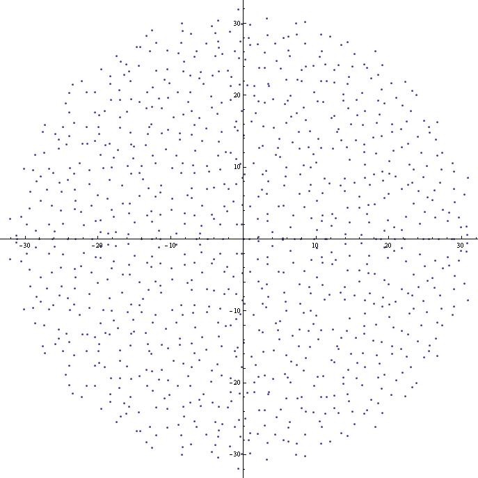
Figure 4: Eigenvalues of 1000-by-1000 matrix with i.i.d Gaussian entries ($\beta=2$)

(from Benedek Valkó’s webpage)

We may then wonder how to quantify the order or rigidity of the configurations according to the temperature. The following result provides some answer, and an improvement at next order on Theorem 8:

Theorem 9 ([SS6]).

Let $A_{n}\subset(\mathbb{R}^{2})^{n}$. Then, for every $\varepsilon>0$ there exists $C_{\varepsilon}$ (bounded when $\varepsilon$ is bounded away from $0$) such that

$$\limsup_{n\to\infty}\frac{1}{n}\log\mathbb{P}_{n}^{\beta}(A_{n})\leq-\beta\Big{(}\frac{|\Sigma|}{\pi}\inf_{P\in A}\int W(E)dP(x,E)-\alpha_{0}-\varepsilon-\frac{C_{\varepsilon}}{\beta}\Big{)},$$

and $A$ is the set of probability measures which are limits (in the weak sense) of blow-ups at rate $\sqrt{n}$ around a point $x$ of the electric fields $\nabla h_{n}$ associated to $\sum_{i=1}^{n}\delta_{{x_{i}}}$ with $(x_{i})\in A_{n}$.

Modulo again the conjecture on $\min W$, this proves crystallization as the temperature goes to $0$: after blowing up around a point $x$ in the support of $\mu_{0}$, at the scale of $\sqrt{n}$, as $\beta\to\infty$ we see (almost surely) a configuration which minimizes $W$. Indeed, $\alpha_{0}$ is the minimum value that $\inf_{P\in A}\int W(E)dP(x,E)$ can possibly take, and is achieved if and only if $W(E)=\min_{\mathcal{A}_{\mu_{0}(x)}}W$ for $P$-a.e. $(x,E)$.

For $\beta$ finite, the result says that the average of $W$ lies below a fixed threshhold (say $\alpha_{0}+1+\frac{C}{\beta}$), except with very small probability.

To our knowledge, this is the first time Coulomb gases are rigorously connected to triangular lattices (again modulo the solution to the conjecture on the minimum of $W$), in agreement with predictions in the literature (cf. [AJ] and references therein).

3 Higher dimensional Coulomb Gases

With Nicolas Rougerie, in [RS], we extended the results for the Coulomb gas presented above to arbitrary higher dimension, considering this time

$$H_{n}(x_{1},\dots,x_{n})=\sum_{i\neq j}g(x_{i}-x_{j})+n\sum_{i=1}^{n}V(x_{i})$$

with $x_{i}\in\mathbb{R}^{d}$ and the kernel $g$ is the Coulomb kernel $-\log|x|$ in dimension $2$ and $|x|^{2-d}$ in dimension $d\geq 3$. The mean-field limit energy is defined in the same way by

$$\mathcal{F}(\mu)=\iint_{\mathbb{R}^{d}\times\mathbb{R}^{d}}g(x-y)\,d\mu(x)\,d\mu(y)+\int_{\mathbb{R}^{d}}V(x)\,d\mu(x).$$

Turning to higher dimension required a new approach and a new definition of $W$, the previous one being very tied to the two-dimensional “ball construction method” as alluded to in Section 2.2. The new approach is based on a different way of renormalizing, or substracting off the infinite “self-interaction” energy of each point: we replace point charges by smeared-out charges, as in “Onsager’s lemma”. More precisely, we pick some arbitrary fixed radial nonnegative function $\rho$, supported in $B(0,1)$ and with integral $1$, and for any point $x$ and $\eta>0$ we introduce the smeared charge

$$\delta_{x}^{(\eta)}=\frac{1}{\eta^{d}}\rho\left(\frac{\cdot}{\eta}\right)*\delta_{x}.$$

Newton’s theorem asserts that the Coulomb potentials generated by the smeared charge $\delta_{x}^{(\eta)}$ and the point charge $\delta_{x}$ coincide outside of $B(x,\eta)$. A consequence of this is that if we define instead of

(28) $$h_{n}^{\prime}(x^{\prime})=-c_{d}\Delta^{-1}\left(\sum_{i=1}^{n}\delta_{x_{i}^{\prime}}-\mu_{0}(x_{0}+x^{\prime}n^{-1/d})\right)$$

as in (21), the potential

(29) $$h_{n,\eta}^{\prime}(x^{\prime})=-c_{d}\Delta^{-1}\left(\sum_{i=1}^{n}\delta_{x_{i}^{\prime}}^{(\eta)}-\mu_{0}(x_{0}+x^{\prime}n^{-1/d})\right)$$

then $h_{n}^{\prime}$ and $h_{n,\eta}^{\prime}$ coincide outside of the $B(x_{i}^{\prime},\eta)$. Moreover, they differ by $\sum_{i}f_{\eta}(x-x_{i}^{\prime})$ where $f_{\eta}$ is a fixed function equal to $c_{d}\Delta^{-1}(\delta_{0}^{(\eta)}-\delta_{0})$, vanishing outside $B(0,\eta)$. (Here the constant $c_{d}$ is the constant such that $-\Delta g=c_{d}\delta_{0}$, depending only on dimension).

By keeping these smeared out charges, we are led at the limit to solutions to

(30) $$-\Delta h_{\eta}=c_{d}\Big{(}\sum_{a}\delta_{a}^{(\eta)}-m\Big{)},\quad m=\mu_{0}(x_{0})$$

which are in bijection with the functions $h$ solving the same equation with $\eta=0$, via adding or subtracting $\sum_{a}f_{\eta}(x-a)$.

For any fixed $\eta>0$ one may then define the electrostatic energy per unit volume of the infinite jellium with smeared charges as

(31) $$\limsup_{R\to\infty}\mathchoice{{\vbox{\hbox{$\textstyle-$}}\kern-4.86108pt}}{{\vbox{\hbox{$\scriptstyle-$}}\kern-3.25pt}}{{\vbox{\hbox{$\scriptscriptstyle-$}}\kern-2.29166pt}}{{\vbox{\hbox{$\scriptscriptstyle-$}}\kern-1.875pt}}\!\int_{K_{R}}|\nabla h_{\eta}|^{2}:=\limsup_{R\to\infty}|K_{R}|^{-1}\int_{K_{R}}|\nabla h_{\eta}|^{2}$$

where $h_{\eta}$ is as in the above definition and $K_{R}$ denotes the cube $[-R,R]^{d}$. This energy is now well-defined for $\eta>0$ and blows up as $\eta\to 0$, since it includes the self-energy of each smeared charge in the collection. One should then “renormalize” (31) by removing the self-energy of each smeared charge before taking the limit $\eta\to 0$. The leading order energy of a smeared charge is $\kappa_{d}g(\eta)$ where $\kappa_{d}$ is a constant depending on dimension and on the choice of the smoothing function $\rho$. We are then led to the definition

Definition 2 ([RS]).

The renormalized energy $\mathcal{W}$ is defined over the class $\mathcal{A}_{m}$ by

$$\mathcal{W}(\nabla h)=\liminf_{\eta\to 0}\mathcal{W}_{\eta}(\nabla h)=\liminf_{\eta\to 0}\left(\limsup_{R\to\infty}\mathchoice{{\vbox{\hbox{$\textstyle-$}}\kern-4.86108pt}}{{\vbox{\hbox{$\scriptstyle-$}}\kern-3.25pt}}{{\vbox{\hbox{$\scriptscriptstyle-$}}\kern-2.29166pt}}{{\vbox{\hbox{$\scriptscriptstyle-$}}\kern-1.875pt}}\!\int_{K_{R}}|\nabla h_{\eta}|^{2}-m(\kappa_{d}g(\eta)+\gamma_{2}\mathbf{1}_{d=2})\right),$$

where $\kappa_{d}$ and $\gamma_{2}$ are constants depending only on the choice of $\rho$.

It is also proven in [RS] that $\mathcal{W}$ achieves its minimum (for each given $m$), which in dimension $2$ coincides with that of $W$. It is also natural to expect that the minimum of $\mathcal{W}$ may be achieved by crystalline configurations (like the FCC lattice in three dimensions) but this is a completely open question.

We are able to show that a similar splitting relation as (23) holds, which makes appear $\mathcal{W}_{\eta}$ instead of $W$. It is however only an inequality, but equality is retrieved as one lets $\eta\to 0$. This allows to let $n\to\infty$ and obtain lower bounds via the same “probabilistic method” mentioned in Section 2.2, for fixed $\eta$. At the end we let $\eta$ tend to $0$, to retrieve similar results as Theorems 7-9.

The following gives the analogue to Theorem 7 but this time expressed in terms of the free energy $F_{n,\beta}=-\frac{2}{\beta}\log Z_{n}^{\beta}$.

Theorem 10 ([RS]).

Let us define

(32) $$\xi_{d}:=\begin{cases}\displaystyle\frac{1}{c_{d}}\left(\min_{\mathcal{A}_{1}}\mathcal{W}\right)\int_{{\mathbb{R}}^{d}}\mu_{0}^{2-2/d}\quad\mbox{if }d\geq 3\\ \displaystyle\frac{1}{2\pi}\min_{\mathcal{A}_{1}}\mathcal{W}-\frac{1}{2}\int_{{\mathbb{R}}^{2}}\mu_{0}\log\mu_{0}\quad\mbox{if }d=2.\end{cases}$$

If $d\geq 3$ and $\beta\geq cn^{2/d-1}$ for some $c>0$ we have, for $n$ large enough, for any $\varepsilon>0$

(33) $$\left|F_{n,\beta}-n^{2}\mathcal{F}(\mu_{0})-n^{2-2/d}\xi_{d}\right|\leq\varepsilon n^{2-2/d}+C_{\varepsilon}\frac{n}{\beta},$$

respectively if $d=2$ and $\beta\geq c(\log n)^{-1}$, $c>0$, for $n$ large enough, for any $\varepsilon>0$,

(34) $$\left|F_{n,\beta}-n^{2}\mathcal{F}(\mu_{0})+\frac{n}{2}\log n-n\xi_{2}\right|\leq\varepsilon n+C_{\varepsilon}\frac{n}{\beta},$$

where $C_{\varepsilon}$ depends only on $\varepsilon$, $V$ and $d$ and is bounded when $\varepsilon$ is bounded away from $0$.

Taking in particular formally $\beta=\infty$ leads to $F_{n,\infty}=\min H_{n}$ and allows to retrieve the next order expansion of $\min H_{n}$.

An analogue of Theorem 9 is also given:

Theorem 11 ([RS]).

For any $n>0$ let $A_{n}\subset(\mathbb{R}^{d})^{n}$. Assume that $\beta\geq cn^{2/d-1}$ for some constant $c>0$. Then for every $\varepsilon>0$, there exists a constant $C_{\varepsilon}$ depending only on $\varepsilon$, $V$, and bounded when $\varepsilon$ is bounded away from $0$, such that we have

(35) $$\limsup_{n\to\infty}\frac{\log\mathbb{P}_{n}^{\beta}(A_{n})}{n^{2-2/d}}\leq-\frac{\beta}{2}\left(\frac{|\Sigma|}{c_{d}}\inf_{P\in A_{\infty}}\int\mathcal{W}(E)dP(x,E)-(\xi_{d}+\varepsilon)-C_{\varepsilon}\lim_{n\to\infty}\frac{n^{2/d-1}}{\beta}\right),$$

where $A$ is the set of probability measures which are limits (in the weak sense) of $\nabla h_{n}^{\prime}(x+\cdot)$ associated to the $(x_{i})\in A_{n}$ via (28).

These results show that the expected regime for crystallization (maybe surprisingly) depends on the dimension and is the regime $\beta\gg n^{2/d-1}$. In that regime, the Gibbs measure essentially concentrates on minimizers of $\mathcal{W}$, which as before would show crystallization if one knew that such minimizers have to be crystalline.

For a self-contained presentation of these topics, one can also refer to [Se4].

Other than proving that specific crystalline configurations achieve the minimum of $W$ or $\mathcal{W}$, the main result missing in these studies is to establish a complete Large Deviations Principle at next order for the Coulomb gas, and identifying the right rate function which should involve $W$, but not only. This would prove at the same time the existence of a complete next order “thermodynamic limit” (for leading order results see [LN] and references therein.

Let us finish by pointing out that the quantum case (of the Coulomb gas) is quite different and studied in [LNSS]: the next order term is of order $n$ and identified to be the ground state of the “Bogoliubov Hamiltonian.”

S. Serfaty
UPMC Univ Paris 06, UMR 7598 Laboratoire Jacques-Louis Lions,
Paris, F-75005 France ;
CNRS, UMR 7598 LJLL, Paris, F-75005 France
& Courant Institute, New York University
251 Mercer st, NY NY 10012, USA.
E-mail: serfaty@ann.jussieu.fr

References

- [A] A. Abrikosov, On the magnetic properties of superconductors of the second type. Soviet Phys. JETP 5 (1957), 1174–1182.
- [AM] M. Aizenman, P. Martin, Structure of Gibbs States of one Dimensional Coulomb Systems, Commun. Math. Phys. 78, (1980) 99-116.
- [AJ] A. Alastuey, B. Jancovici, On the classical two-dimensional one-component Coulomb plasma. J. Physique 42 (1981), no. 1, 1–12.
- [AOC] Y. Ameur, J. Ortega-Cerdà, Beurling-Landau densities of weighted Fekete sets and correlation kernel estimates, J. Funct. Anal. 263 (2012), no. 7, 1825–1861.
- [BJOS1] S. Baldo, R. L. Jerrard, G. Orlandi, H. M. Soner, Vortex density models for superconductivity and superfluidity. Comm. Math. Phys. 318, (2013), no. 1, 131–171.
- [BJOS2] S. Baldo, R. L. Jerrard, G. Orlandi, H.M. Soner, Convergence of Ginzburg-Landau functionals in three-dimensional superconductivity. Arch. Ration. Mech. Anal. 205 (2012), no. 3, 699–752.
- [BL] H. J. Brascamp, E. H. Lieb: In: Functional integration and its applications. A.M. Arthurs (ed.). Clarendon Press, 1975.
- [BZ] G. Ben Arous, O. Zeitouni, Large deviations from the circular law. ESAIM Probab. Statist. 2 (1998), 123 –134.
- [BBH] F. Bethuel, H. Brezis, F. Hélein, Ginzburg-Landau Vortices, Progress in Nonlinear Partial Differential Equations and Their Applications, Birkhäuser, 1994.
- [BOS2] F. Bethuel, G. Orlandi, D. Smets, Collisions and phase-vortex interactions in dissipative Ginzburg-Landau dynamics, Duke Math. J. 130 (2005), 523–614.
- [BOS3] F. Bethuel, G. Orlandi, D. Smets, Quantization and motion law for Ginzburg-Landau vortices, Arch. Ration. Mech. Anal. 183 (2007), 315–370.
- [BOS4] F. Bethuel, G. Orlandi, D. Smets, Dynamics of multiple degree Ginzburg-Landau vortices, Comm. Math. Phys. 272 (2007), 229–261
- [BR1] F. Bethuel, T. Rivière, Vortices for a variational problem related to superconductivity. Ann. Inst. H. Poincaré Anal. Non Linéaire 12 (1995), no. 3, 243–303.
- [BR2] F. Bethuel, T. Rivière, Vorticité dans les modèles de Ginzburg-Landau pour la supraconductivité, Séminaire sur les équations aux Dérivées Partielles, 1993–1994, Exp. No. XVI, École Polytech., Palaiseau, 1994.
- [BPT] D. Bourne, M. Peletier, F. Theil, Nonlocal problems and the minimality of the triangular lattice, arXiv:1212.6973.
- [BS] A. Borodin, S. Serfaty, Renormalized Energy Concentration in Random Matrices, Comm. Math. Phys. 320, no. 1, (2013), 199-244.
- [Br] A. Braides, -convergence for beginners. Oxford Lecture Series in Mathematics and its Applications, 22. Oxford University Press, Oxford, 2002.
- [Ch] S. J. Chapman, A hierarchy of models for type-II superconductors. SIAM Rev. 42 (2000), no. 4, 555–598.
- [CS] A. Contreras, S. Serfaty, Large Vorticity Stable Solutions to the Ginzburg-Landau Equations, to appear in Indiana Univ. Math. J.
- [DM] G. Dal Maso, An introduction to -convergence, Progress in Nonlinear Differential Equations and their Applications, 8. Birkhäuser Boston, Inc., Boston, MA, 1993.
- [DGP] Q. Du, M. Gunzburger, J. S. Peterson, Analysis and approximation of the Ginzburg-Landau model of superconductivity. SIAM Rev. 34 (1992), no. 1, 54–81.
- [Dy] F. Dyson, Statistical theory of the energy levels of a complex system. Part I, J. Math. Phys. 3, 140–156 (1962); Part II, ibid. 157 165; Part III, ibid. 166–175
- [CPRY] M. Correggi, F. Pinsker, N. Rougerie and J. Yngvason, Critical Rotational Speeds in the Gross-Pitaevskii Theory on a Disc with Dirichlet Boundary Conditions, J. Stat. Phys. 143 (2011), no. 2, 261–305.
- [Fo] P. J. Forrester, Log-gases and random matrices. London Mathematical Society Monographs Series, 34. Princeton University Press, 2010.
- [GL] V. L. Ginzburg, L. D. Landau, Collected papers of L.D.Landau. Edited by D. Ter. Haar, Pergamon Press, Oxford 1965.
- [DeG] P. G. De Gennes, Superconductivity of metal and alloys. Benjamin, New York and Amsterdam, 1966.
- [FH] S. Fournais, B. Helffer, Spectral Methods in Surface Superconductivity, Progress in Nonlinear Differential Equations 77, Birkhäuser, 2010.
- [GP] T. Giorgi, D. Phillips, The breakdown of superconductivity due to strong fields for the Ginzburg-Landau model. SIAM J. Math. Anal. 30 (1999), no. 2, 341–359.
- [GMS1] D. Goldman, C. Muratov, S. Serfaty, The -limit of the two-dimensional Ohta-Kawasaki energy. I. Droplet density, to appear in Arch. Rat. Mech. Anal.
- [GMS2] D. Goldman, C. Muratov, S. Serfaty, The -limit of the two-dimensional Ohta-Kawasaki energy. II. Droplet arrangement via the renormalized energy, arXiv:1210.5098.
- [GS] S. Gueron, I. Shafrir, On a Discrete Variational Problem Involving Interacting Particles. SIAM J. Appl. Math. 60 (2000), no. 1, 1–17.
- [Ja] B. Jancovici, Exact results for the two-dimensional one-component plasma, Phys. Rev. Lett. 46 (1981), 263–280.
- [JLM] B. Jancovici, J. Lebowitz, G. Manificat, Large charge fluctuations in classical Coulomb systems. J. Statist. Phys. 72 (1993), no. 3-4, 773–787.
- [Je] R. L. Jerrard, Lower bounds for generalized Ginzburg-Landau functionals. SIAM J. Math. Anal. 30 (1999), no. 4, 721-746.
- [JS] R. L. Jerrard, H. M. Soner, Dynamics of Ginzburg-Landau vortices. Arch. Ration. Mech. Anal. 142 (1998), no. 2, 99–125.
- [Ka] A. Kachmar, The ground state energy of the three-dimensional Ginzburg-Landau model in the mixed phase. J. Funct. Anal. 261 (11), (2011) 3328–3344.
- [Ku] H. Kunz, The One-Dimensional Classical Electron Gas, Ann. Phys. 85, 303–335 (1974).
- [KS] M. Kurzke, D. Spirn, Vortex liquids and the Ginzburg-Landau equation, preprint.
- [Le] A. Lenard, Exact statistical mechanics of a one-dimensional system with Coulomb forces. III. Statistics of the electric field, J. Math. Phys. 4, (1963), 533-543.
- [LN] E. H. Lieb, H. Narnhofer, The thermodynamic limit for jellium, J. Statist. Phys. 12, 291–310 (1975).
- [Lin] F. H. Lin, Some dynamic properties of Ginzburg-Landau vortices. Comm. Pure Appl. Math. 49 (1996), 323–359.
- [LNSS] M. Lewin, P.T. Nam, S. Serfaty, J.P. Solovej, Bogoliubov Spectrum of interaction Bose gases, to appear in Comm. Pure Appl. Math.
- [Mo] H. L. Montgomery, Minimal Theta functions. Glasgow Math J. 30, (1988), No. 1, 75-85, (1988).
- [PH] D. Petz, F. Hiai, Logarithmic energy as an entropy functional. Advances in differential equations and mathematical physics, 205–221, Contemp. Math., 217, Amer. Math. Soc., Providence, RI, 1998.
- [Ra] C. Radin, The ground state for soft disks. J. Statist. Phys., 26 (1981), 365–373.
- [RNS] S. Rota Nodari, S. Serfaty, Renormalized Energy Equidistribution and Local Charge Balance in 2D Coulomb Systems, arXiv:1307.3363.
- [RS] N. Rougerie, S. Serfaty, Higher Dimensional Coulomb Gases and Renormalized Energy Functionals. arXiv:1307.2805.
- [Ri] T. Rivière, Line vortices in the -Higgs model. ESAIM Contrôl Optim. Calc. Var. 1 (1995/1996), 77–167.
- [ST] E. Saff, V. Totik, Logarithmic potentials with external fields, Springer-Verlag, 1997.
- [Sa] E. Sandier, Lower bounds for the energy of unit vector fields and applications. J. Funct. Anal. 152 (1998), No. 2, 379–403.
- [SS1] E. Sandier, S. Serfaty, Vortices in the Magnetic Ginzburg-Landau Model, Birkhäuser, 2007.
- [SS2] E. Sandier, S. Serfaty, A rigorous derivation of a free-boundary problem arising in superconductivity. Ann. Sci. École Norm. Sup. (4) 33 (2000), no. 4, 561–592.
- [SS3] E. Sandier, S. Serfaty, Limiting vorticities for the Ginzburg-Landau equations. Duke Math. J. 117 (2003), no. 3, 403-446.
- [SS4] E. Sandier, S. Serfaty, Gamma-convergence of gradient flows with applications to Ginzburg-Landau, Comm. Pure Appl. Math, 57 (2004), 1627–1672.
- [SS5] E. Sandier, S. Serfaty, From the Ginzburg-Landau model to vortex lattice problems, Comm. Math. Phys. 313 (2012), no. 3, 635-743.
- [SS6] E. Sandier, S. Serfaty, 2D Coulomb gases and the Renormalized Energy, arXiv:1201.3503.
- [SS7] E. Sandier, S. Serfaty, 1D Log gases and the Renormalized Energy: Crystallization at Vanishing Temperature, arXiv:1303.2968.
- [SM] R. Sari, D. Merlini, On the -dimensional one-component classical plasma: the thermodynamic limit problem revisited. J. Statist. Phys. 14 (1976), no. 2, 91–100.
- [Se1] S. Serfaty, Local minimizers for the Ginzburg-Landau energy near critical magnetic field, part I. Comm. Contemp. Math. 1 (1999), no. 2, 213–254; part II, 295–333.
- [Se2] S. Serfaty, Stable configurations in superconductivity: uniqueness, multiplicity and vortex-nucleation. Arch. Ration. Mech. Anal. 149 (1999), 329–365.
- [Se3] S. Serfaty, Vortex collisions and energy-dissipation rates in the Ginzburg-Landau heat flow. Part I: Study of the perturbed Ginzburg-Landau equation, Journal Eur. Math Society, 9 (2007), 177–217, Part II: The dynamics, Journal Eur. Math Society, 9 (2007), 383–426.
- [Se4] S. Serfaty, Coulomb Gases and Ginzburg-Landau Vortices, Zurich Lecture Notes in Mathematics, Eur. Math. Soc., forthcoming.
- [Sp1] D. Spirn, Vortex dynamics of the full time-dependent Ginzburg-Landau equations. Comm. Pure Appl. Math. 55 (2002), no. 5, 537–581.
- [Sp2] D. Spirn, Vortex motion law for the Schrödinger-Ginzburg-Landau equations. SIAM J. Math. Anal. 34 (2003), no. 6, 1435–1476.
- [Th] F. Theil, A proof of crystallization in two dimensions. Comm. Math. Phys., 262 (2006), 209–236.
- [T] M. Tinkham, Introduction to superconductivity. Second edition. McGraw-Hill, New York, 1996.
- [Wi] E. Wigner, Characteristic vectors of bordered matrices with infinite dimensions, Ann. Math. 62, 548–564 (1955).