1. Introduction
In several fields of sciences like geophysics, astrophysics, climatology etc.
we come across observations which are non-Gaussian . A Gaussian process is
characterized by its first two moments, namely, mean, variance and
autocorrelations (or equivalently second order spectrum). There are several
clearly different processes having identical second-order properties
[SR97 ] , [IT97 ] , [Dig13 ] but their
distributions is not Gaussian and they are clearly different, therefore it is
necessary to study higher order structures. Although second order properties
of Gaussian fields are well established, see [Yag87 ] ,
[Yad83 ] , [Adl10 ] , [Bri01 ] ,
[Ros00 ] , [Ros85 ] , [Pri88 ] ,
[Leo89 ] , [BH86 ] ,
[LS12 ] , [Mok07 ] ,
[Mok08 ] . Characterization of non-Gaussian fields which require
study of higher order moments (or equivalently higher order spectra) are not
well known. The isotropy of stochastic phenomenons in two dimensions has been
established in several applications, [NY97 ] ,
[OT96 ] . Only recently has been made quite a number of
steps toward the statistical investigation of non-Gaussian isotropic fields,
mainly for understanding the Cosmic Microwave Background (CMB) anisotropies
[OH02 ] , [AH12 ] .
In this paper our object is to continue the frequency domain investigations
published in our paper [Ter14 ] , where additional to the
covarinace and the spectrum the connection between the bicovariance and the
bispectrum has been studied in details. Here the trispectrum and all higher
order spectra of such fields are described in terms of Bessel functions. The
connection between the tricovariance and the trispectrum is similar to the one
between the bicovariance and the bispectrum It was necessary to prove some
particular integrals of Bessel functions, given in terms of sides and angles
of a multilateral.
1.1. Isotropy
A homogenous real valued stochastic field X ( x ¯ ) 𝑋 ¯ 𝑥 X\left(\underline{x}\right) x ¯ ∈ ℝ 2 ¯ 𝑥 superscript ℝ 2 \underline{x}\in\mathbb{R}^{2}
X ( x ¯ ) = ∫ ℝ 2 e i x ¯ ⋅ ω ¯ Z ( d ω ¯ ) , ω ¯ , x ¯ ∈ ℝ 2 , formulae-sequence 𝑋 ¯ 𝑥 subscript superscript ℝ 2 superscript 𝑒 ⋅ 𝑖 ¯ 𝑥 ¯ 𝜔 𝑍 𝑑 ¯ 𝜔 ¯ 𝜔
¯ 𝑥 superscript ℝ 2 X\left(\underline{x}\right)=\int_{\mathbb{R}^{2}}e^{i\underline{x}\cdot\underline{\omega}}Z\left(d\underline{\omega}\right),\quad\underline{\omega},\underline{x}\in\mathbb{R}^{2},
with E X ( x ¯ ) = 0 𝐸 𝑋 ¯ 𝑥 0 EX\left(\underline{x}\right)=0 Z ( d ω ¯ ) 𝑍 𝑑 ¯ 𝜔 Z\left(d\underline{\omega}\right) E | Z ( d ω ¯ ) | 2 = F 0 ( d ω ¯ ) 𝐸 superscript 𝑍 𝑑 ¯ 𝜔 2 subscript 𝐹 0 𝑑 ¯ 𝜔 E\left|Z\left(d\underline{\omega}\right)\right|^{2}=F_{0}\left(d\underline{\omega}\right) X ( x ¯ ) 𝑋 ¯ 𝑥 X\left(\underline{x}\right) [Yag87 ] for details. We can rewrite X ( x ¯ ) 𝑋 ¯ 𝑥 X\left(\underline{x}\right)
X ( r , φ ) = ∫ 0 ∞ ∫ 0 2 π e i ρ r cos ( φ − η ) Z ( ρ d ρ d η ) 𝑋 𝑟 𝜑 superscript subscript 0 superscript subscript 0 2 𝜋 superscript 𝑒 𝑖 𝜌 𝑟 𝜑 𝜂 𝑍 𝜌 𝑑 𝜌 𝑑 𝜂 X\left(r,\varphi\right)=\int_{0}^{\infty}\int_{0}^{2\pi}e^{i\rho r\cos\left(\varphi-\eta\right)}Z\left(\rho d\rho d\eta\right)
where x ¯ = ( r , φ ) ¯ 𝑥 𝑟 𝜑 \underline{x}=\left(r,\varphi\right) ω ¯ = ( ρ , η ) ¯ 𝜔 𝜌 𝜂 \underline{\omega}=\left(\rho,\eta\right) r = | x ¯ | = x 1 2 + x 2 2 𝑟 ¯ 𝑥 superscript subscript 𝑥 1 2 superscript subscript 𝑥 2 2 r=\left|\underline{x}\right|=\sqrt{x_{1}^{2}+x_{2}^{2}} ρ = | ω ¯ | 𝜌 ¯ 𝜔 \rho=\left|\underline{\omega}\right| x ¯ ⋅ ω ¯ = r ρ cos ( φ − η ) ⋅ ¯ 𝑥 ¯ 𝜔 𝑟 𝜌 𝜑 𝜂 \underline{x}\cdot\underline{\omega}=r\rho\cos\left(\varphi-\eta\right) F 0 ( d ω ¯ ) subscript 𝐹 0 𝑑 ¯ 𝜔 F_{0}\left(d\underline{\omega}\right) F 0 ( d ω ¯ ) = E | Z ( d ω ¯ ) | 2 = E | Z ( ρ d ρ d η ) | 2 = F ( ρ d ρ ) d η subscript 𝐹 0 𝑑 ¯ 𝜔 𝐸 superscript 𝑍 𝑑 ¯ 𝜔 2 𝐸 superscript 𝑍 𝜌 𝑑 𝜌 𝑑 𝜂 2 𝐹 𝜌 𝑑 𝜌 𝑑 𝜂 F_{0}\left(d\underline{\omega}\right)=E\left|Z\left(d\underline{\omega}\right)\right|^{2}=E\left|Z\left(\rho d\rho d\eta\right)\right|^{2}=F\left(\rho d\rho\right)d\eta g ∈ S O ( 2 ) 𝑔 𝑆 𝑂 2 g\in SO\left(2\right) γ 𝛾 \gamma x ¯ ∈ ℝ 2 ¯ 𝑥 superscript ℝ 2 \underline{x}\in\mathbb{R}^{2} x ¯ = ( r , φ ) ¯ 𝑥 𝑟 𝜑 \underline{x}=\left(r,\varphi\right) g x ¯ = ( r , φ − γ ) 𝑔 ¯ 𝑥 𝑟 𝜑 𝛾 g\underline{x}=\left(r,\varphi-\gamma\right) Λ ( g ) Λ 𝑔 \Lambda\left(g\right) f ( r , φ ) 𝑓 𝑟 𝜑 f\left(r,\varphi\right) Λ ( g ) f ( r , φ ) = f ( g − 1 ( r , φ ) ) = f ( r , φ + γ ) Λ 𝑔 𝑓 𝑟 𝜑 𝑓 superscript 𝑔 1 𝑟 𝜑 𝑓 𝑟 𝜑 𝛾 \Lambda\left(g\right)f\left(r,\varphi\right)=f\left(g^{-1}\left(r,\varphi\right)\right)=f\left(r,\varphi+\gamma\right)
The invariance of the covariance function is satisfactory for Gaussian cases
but for non-Gaussian fields we need invariance of higher order cumulants as well.
Definition 1 .
A homogenous stochastic field X ( x ¯ ) 𝑋 ¯ 𝑥 X\left(\underline{x}\right) X ( x ¯ ) 𝑋 ¯ 𝑥 X\left(\underline{x}\right)
As far as the homogenous field X ( x ¯ ) 𝑋 ¯ 𝑥 X\left(\underline{x}\right) F 0 ( d ω ¯ ) subscript 𝐹 0 𝑑 ¯ 𝜔 F_{0}\left(d\underline{\omega}\right) F 0 ( d ω ¯ ) = F ( ρ d ρ ) d η subscript 𝐹 0 𝑑 ¯ 𝜔 𝐹 𝜌 𝑑 𝜌 𝑑 𝜂 F_{0}\left(d\underline{\omega}\right)=F\left(\rho d\rho\right)d\eta
Cov ( Λ ( g ) X ( x ¯ 1 ) , Λ ( g ) X ( x ¯ 2 ) ) = Cov ( X ( x ¯ 1 ) , X ( x ¯ 2 ) ) , Cov Λ 𝑔 𝑋 subscript ¯ 𝑥 1 Λ 𝑔 𝑋 subscript ¯ 𝑥 2 Cov 𝑋 subscript ¯ 𝑥 1 𝑋 subscript ¯ 𝑥 2 \operatorname*{Cov}\left(\Lambda\left(g\right)X\left(\underline{x}_{1}\right),\Lambda\left(g\right)X\left(\underline{x}_{2}\right)\right)=\operatorname*{Cov}\left(X\left(\underline{x}_{1}\right),X\left(\underline{x}_{2}\right)\right),
for each x ¯ 1 subscript ¯ 𝑥 1 \underline{x}_{1} x ¯ 2 subscript ¯ 𝑥 2 \underline{x}_{2} g ∈ S O ( 2 ) 𝑔 𝑆 𝑂 2 g\in SO\left(2\right) X ( x ¯ ) 𝑋 ¯ 𝑥 X\left(\underline{x}\right)
Let us consider a homogenous and isotropic stochastic field X ( x ¯ ) = X ( r , φ ) 𝑋 ¯ 𝑥 𝑋 𝑟 𝜑 X\left(\underline{x}\right)=X\left(r,\varphi\right) r > 0 𝑟 0 r>0 φ ∈ [ 0 , 2 π ) 𝜑 0 2 𝜋 \varphi\in\left[0,2\pi\right) [Ter14 ]
(1.1) X ( r , φ ) = ∑ ℓ = − ∞ ∞ e i ℓ φ ∫ 0 ∞ J ℓ ( ρ r ) Z ℓ ( ρ d ρ ) , 𝑋 𝑟 𝜑 superscript subscript ℓ superscript 𝑒 𝑖 ℓ 𝜑 superscript subscript 0 subscript 𝐽 ℓ 𝜌 𝑟 subscript 𝑍 ℓ 𝜌 𝑑 𝜌 X\left(r,\varphi\right)=\sum_{\ell=-\infty}^{\infty}e^{i\ell\varphi}\int_{0}^{\infty}J_{\ell}\left(\rho r\right)Z_{\ell}\left(\rho d\rho\right),
where J ℓ subscript 𝐽 ℓ J_{\ell}
(1.2) Z ℓ ( ρ d ρ ) = ∫ 0 2 π i ℓ e − i ℓ η Z ( ρ d ρ d η ) . subscript 𝑍 ℓ 𝜌 𝑑 𝜌 superscript subscript 0 2 𝜋 superscript 𝑖 ℓ superscript 𝑒 𝑖 ℓ 𝜂 𝑍 𝜌 𝑑 𝜌 𝑑 𝜂 Z_{\ell}\left(\rho d\rho\right)=\int_{0}^{2\pi}i^{\ell}e^{-i\ell\eta\ }Z\left(\rho d\rho d\eta\right).
Z ℓ subscript 𝑍 ℓ Z_{\ell}
Cov ( Z ℓ 1 ( ρ 1 d ρ 1 ) , Z ℓ 2 ( ρ 2 d ρ 2 ) ) = δ ℓ 1 − ℓ 2 F ( ρ d ρ ) , Cov subscript 𝑍 subscript ℓ 1 subscript 𝜌 1 𝑑 subscript 𝜌 1 subscript 𝑍 subscript ℓ 2 subscript 𝜌 2 𝑑 subscript 𝜌 2 subscript 𝛿 subscript ℓ 1 subscript ℓ 2 𝐹 𝜌 𝑑 𝜌 \operatorname*{Cov}\left(Z_{\ell_{1}}\left(\rho_{1}d\rho_{1}\right),Z_{\ell_{2}}\left(\rho_{2}d\rho_{2}\right)\right)=\delta_{\ell_{1}-\ell_{2}}F\left(\rho d\rho\right),
where δ ℓ subscript 𝛿 ℓ \delta_{\ell} δ 𝛿 \delta F ( ρ d ρ ) 𝐹 𝜌 𝑑 𝜌 F\left(\rho d\rho\right) Z ℓ ( ρ d ρ ) subscript 𝑍 ℓ 𝜌 𝑑 𝜌 Z_{\ell}\left(\rho d\rho\right) ℓ ℓ \ell 1.1 e i ℓ φ superscript 𝑒 𝑖 ℓ 𝜑 e^{i\ell\varphi} ℓ ℓ \ell X ( x ¯ ) 𝑋 ¯ 𝑥 X\left(\underline{x}\right)
The isotropy of X ( r , φ ) 𝑋 𝑟 𝜑 X\left(r,\varphi\right) X ( r , φ ) 𝑋 𝑟 𝜑 X\left(r,\varphi\right) g ∈ S O ( 2 ) 𝑔 𝑆 𝑂 2 g\in SO\left(2\right)
Λ ( g ) X ( r , φ ) Λ 𝑔 𝑋 𝑟 𝜑 \displaystyle\Lambda\left(g\right)X\left(r,\varphi\right) = ∑ ℓ = − ∞ ∞ e i ℓ φ ∫ 0 ∞ J ℓ ( ρ r ) e i ℓ γ Z ℓ ( ρ d ρ ) absent superscript subscript ℓ superscript 𝑒 𝑖 ℓ 𝜑 superscript subscript 0 subscript 𝐽 ℓ 𝜌 𝑟 superscript 𝑒 𝑖 ℓ 𝛾 subscript 𝑍 ℓ 𝜌 𝑑 𝜌 \displaystyle=\sum_{\ell=-\infty}^{\infty}e^{i\ell\varphi}\int_{0}^{\infty}J_{\ell}\left(\rho r\right)e^{i\ell\gamma}Z_{\ell}\left(\rho d\rho\right)
= ∑ ℓ = − ∞ ∞ e i ℓ φ ∫ 0 ∞ J ℓ ( ρ r ) Z ℓ ( ρ d ρ ) , absent superscript subscript ℓ superscript 𝑒 𝑖 ℓ 𝜑 superscript subscript 0 subscript 𝐽 ℓ 𝜌 𝑟 subscript 𝑍 ℓ 𝜌 𝑑 𝜌 \displaystyle=\sum_{\ell=-\infty}^{\infty}e^{i\ell\varphi}\int_{0}^{\infty}J_{\ell}\left(\rho r\right)Z_{\ell}\left(\rho d\rho\right),
hence the distribution of Z ℓ ( ρ d ρ ) subscript 𝑍 ℓ 𝜌 𝑑 𝜌 Z_{\ell}\left(\rho d\rho\right) e i ℓ γ Z ℓ ( ρ d ρ ) superscript 𝑒 𝑖 ℓ 𝛾 subscript 𝑍 ℓ 𝜌 𝑑 𝜌 e^{i\ell\gamma}Z_{\ell}\left(\rho d\rho\right)
Cum ( Z ℓ 1 ( ρ 1 d ρ 1 ) , Z ℓ 2 ( ρ 2 d ρ 2 ) ) = e i ( ℓ 1 + ℓ 2 ) γ Cum ( Z ℓ 1 ( ρ 1 d ρ 1 ) , Z ℓ 2 ( ρ 2 d ρ 2 ) ) , Cum subscript 𝑍 subscript ℓ 1 subscript 𝜌 1 𝑑 subscript 𝜌 1 subscript 𝑍 subscript ℓ 2 subscript 𝜌 2 𝑑 subscript 𝜌 2 superscript 𝑒 𝑖 subscript ℓ 1 subscript ℓ 2 𝛾 Cum subscript 𝑍 subscript ℓ 1 subscript 𝜌 1 𝑑 subscript 𝜌 1 subscript 𝑍 subscript ℓ 2 subscript 𝜌 2 𝑑 subscript 𝜌 2 \operatorname*{Cum}\left(Z_{\ell_{1}}\left(\rho_{1}d\rho_{1}\right),Z_{\ell_{2}}\left(\rho_{2}d\rho_{2}\right)\right)=e^{i\left(\ell_{1}+\ell_{2}\right)\gamma}\operatorname*{Cum}\left(Z_{\ell_{1}}\left(\rho_{1}d\rho_{1}\right),Z_{\ell_{2}}\left(\rho_{2}d\rho_{2}\right)\right),
for each γ 𝛾 \gamma ℓ 1 + ℓ 2 = 0 subscript ℓ 1 subscript ℓ 2 0 \ell_{1}+\ell_{2}=0 Cum ( Z ℓ 1 ( ρ 1 d ρ 1 ) , Z ℓ 2 ( ρ 2 d ρ 2 ) ) = 0 Cum subscript 𝑍 subscript ℓ 1 subscript 𝜌 1 𝑑 subscript 𝜌 1 subscript 𝑍 subscript ℓ 2 subscript 𝜌 2 𝑑 subscript 𝜌 2 0 \operatorname*{Cum}\left(Z_{\ell_{1}}\left(\rho_{1}d\rho_{1}\right),Z_{\ell_{2}}\left(\rho_{2}d\rho_{2}\right)\right)=0
Cum ( Z ℓ 1 ( ρ 1 d ρ 1 ) , … , Z ℓ p ( ρ p d ρ p ) ) = e i ( ℓ 1 + ℓ 2 ⋯ + ℓ p ) γ Cum ( Z ℓ 1 ( ρ 1 d ρ 1 ) , … , Z ℓ p ( ρ p d ρ p ) ) , Cum subscript 𝑍 subscript ℓ 1 subscript 𝜌 1 𝑑 subscript 𝜌 1 … subscript 𝑍 subscript ℓ 𝑝 subscript 𝜌 𝑝 𝑑 subscript 𝜌 𝑝 superscript 𝑒 𝑖 subscript ℓ 1 subscript ℓ 2 ⋯ subscript ℓ 𝑝 𝛾 Cum subscript 𝑍 subscript ℓ 1 subscript 𝜌 1 𝑑 subscript 𝜌 1 … subscript 𝑍 subscript ℓ 𝑝 subscript 𝜌 𝑝 𝑑 subscript 𝜌 𝑝 \operatorname*{Cum}\left(Z_{\ell_{1}}\left(\rho_{1}d\rho_{1}\right),\ldots,Z_{\ell_{p}}\left(\rho_{p}d\rho_{p}\right)\right)=e^{i\left(\ell_{1}+\ell_{2}\cdots+\ell_{p}\right)\gamma}\operatorname*{Cum}\left(Z_{\ell_{1}}\left(\rho_{1}d\rho_{1}\right),\ldots,Z_{\ell_{p}}\left(\rho_{p}d\rho_{p}\right)\right),
that is either ℓ 1 + ℓ 2 ⋯ + ℓ p = 0 subscript ℓ 1 subscript ℓ 2 ⋯ subscript ℓ 𝑝 0 \ell_{1}+\ell_{2}\cdots+\ell_{p}=0 Cum ( Z ℓ 1 ( ρ 1 d ρ 1 ) , Z ℓ 2 ( ρ 2 d ρ 2 ) , … , Z ℓ p ( ρ p d ρ p ) ) = 0 Cum subscript 𝑍 subscript ℓ 1 subscript 𝜌 1 𝑑 subscript 𝜌 1 subscript 𝑍 subscript ℓ 2 subscript 𝜌 2 𝑑 subscript 𝜌 2 … subscript 𝑍 subscript ℓ 𝑝 subscript 𝜌 𝑝 𝑑 subscript 𝜌 𝑝 0 \operatorname*{Cum}\left(Z_{\ell_{1}}\left(\rho_{1}d\rho_{1}\right),Z_{\ell_{2}}\left(\rho_{2}d\rho_{2}\right),\ldots,Z_{\ell_{p}}\left(\rho_{p}d\rho_{p}\right)\right)=0 p 𝑝 p Cum ( Z ℓ 1 ( ρ 1 d ρ 1 ) , … , Z ℓ p ( ρ p d ρ p ) ) Cum subscript 𝑍 subscript ℓ 1 subscript 𝜌 1 𝑑 subscript 𝜌 1 … subscript 𝑍 subscript ℓ 𝑝 subscript 𝜌 𝑝 𝑑 subscript 𝜌 𝑝 \operatorname*{Cum}\left(Z_{\ell_{1}}\left(\rho_{1}d\rho_{1}\right),\ldots,Z_{\ell_{p}}\left(\rho_{p}d\rho_{p}\right)\right) X ( r , φ ) 𝑋 𝑟 𝜑 X\left(r,\varphi\right)
1.2. Spectrum and Bispectrum
It is well known from theory of Gaussian fields that
Cov ( X ( x ¯ ) , X ( y ¯ ) ) = ∫ 0 ∞ J 0 ( ρ r ) F ( ρ d ρ ) , Cov 𝑋 ¯ 𝑥 𝑋 ¯ 𝑦 superscript subscript 0 subscript 𝐽 0 𝜌 𝑟 𝐹 𝜌 𝑑 𝜌 \operatorname*{Cov}\left(X\left(\underline{x}\right),X\left(\underline{y}\right)\right)=\int_{0}^{\infty}J_{0}\left(\rho r\right)F\left(\rho d\rho\right),
where r = | x ¯ − y ¯ | 𝑟 ¯ 𝑥 ¯ 𝑦 r=\left|\underline{x}-\underline{y}\right| [Yad83 ] , [Yag87 ] , [Bri74 ] . The covariances
and the spectral measure uniquely define each other since the Hankel transform
gives the inverse. For absolutely continuos spectral measure we have F ( ρ d ρ ) = σ 2 | A ( ρ ) | 2 ρ d ρ 𝐹 𝜌 𝑑 𝜌 superscript 𝜎 2 superscript 𝐴 𝜌 2 𝜌 𝑑 𝜌 F\left(\rho d\rho\right)=\sigma^{2}\left|A\left(\rho\right)\right|^{2}\rho d\rho
𝒞 2 ( r ) subscript 𝒞 2 𝑟 \displaystyle\mathcal{C}_{2}\left(r\right) = ∫ 0 ∞ J 0 ( ρ r ) σ 2 | A ( ρ ) | 2 ρ 𝑑 ρ , absent superscript subscript 0 subscript 𝐽 0 𝜌 𝑟 superscript 𝜎 2 superscript 𝐴 𝜌 2 𝜌 differential-d 𝜌 \displaystyle=\int_{0}^{\infty}J_{0}\left(\rho r\right)\sigma^{2}\left|A\left(\rho\right)\right|^{2}\rho d\rho,
σ 2 | A ( ρ ) | 2 superscript 𝜎 2 superscript 𝐴 𝜌 2 \displaystyle\sigma^{2}\left|A\left(\rho\right)\right|^{2} = 1 2 π ∫ 0 ∞ J 0 ( ρ r ) 𝒞 2 ( r ) r 𝑑 r , absent 1 2 𝜋 superscript subscript 0 subscript 𝐽 0 𝜌 𝑟 subscript 𝒞 2 𝑟 𝑟 differential-d 𝑟 \displaystyle=\frac{1}{2\pi}\int_{0}^{\infty}J_{0}\left(\rho r\right)\mathcal{C}_{2}\left(r\right)rdr,
where 𝒞 2 ( r ) = Cov ( X ( x ¯ ) , X ( y ¯ ) ) subscript 𝒞 2 𝑟 Cov 𝑋 ¯ 𝑥 𝑋 ¯ 𝑦 \mathcal{C}_{2}\left(r\right)=\operatorname*{Cov}\left(X\left(\underline{x}\right),X\left(\underline{y}\right)\right) r = | x ¯ − y ¯ | 𝑟 ¯ 𝑥 ¯ 𝑦 r=\left|\underline{x}-\underline{y}\right|
The third order structure of a homogenous and isotropic stochastic field
X ( x ¯ ) 𝑋 ¯ 𝑥 X\left(\underline{x}\right) X ( x ¯ ) 𝑋 ¯ 𝑥 X\left(\underline{x}\right)
(1.3) Cum ( X ( x ¯ 1 ) , X ( x ¯ 2 ) , X ( x ¯ 3 ) ) = Cum ( X ( g ( x ¯ 1 − x ¯ 3 ) ) X ( | x ¯ 2 − x ¯ 3 | n ¯ ) , X ( 0 ) ) Cum 𝑋 subscript ¯ 𝑥 1 𝑋 subscript ¯ 𝑥 2 𝑋 subscript ¯ 𝑥 3 Cum 𝑋 𝑔 subscript ¯ 𝑥 1 subscript ¯ 𝑥 3 𝑋 subscript ¯ 𝑥 2 subscript ¯ 𝑥 3 ¯ 𝑛 𝑋 0 \operatorname*{Cum}\left(X\left(\underline{x}_{1}\right),X\left(\underline{x}_{2}\right),X\left(\underline{x}_{3}\right)\right)=\operatorname*{Cum}\left(X\left(g\left(\underline{x}_{1}-\underline{x}_{3}\right)\right)X\left(\left|\underline{x}_{2}-\underline{x}_{3}\right|\underline{n}\right),X\left(0\right)\right)
where g 𝑔 g x ¯ 2 − x ¯ 3 subscript ¯ 𝑥 2 subscript ¯ 𝑥 3 \underline{x}_{2}-\underline{x}_{3} n ¯ = ( 0 , 1 ) ¯ 𝑛 0 1 \underline{n}=\left(0,1\right) Z ( d ω ¯ ) 𝑍 𝑑 ¯ 𝜔 Z\left(d\underline{\omega}\right) X ( x ¯ ) 𝑋 ¯ 𝑥 X\left(\underline{x}\right)
Cum ( Z ( d ω ¯ 1 ) , Z ( d ω ¯ 2 ) , Z ( d ω ¯ 3 ) ) Cum 𝑍 𝑑 subscript ¯ 𝜔 1 𝑍 𝑑 subscript ¯ 𝜔 2 𝑍 𝑑 subscript ¯ 𝜔 3 \displaystyle\operatorname*{Cum}\left(Z\left(d\underline{\omega}_{1}\right),Z\left(d\underline{\omega}_{2}\right),Z\left(d\underline{\omega}_{3}\right)\right) = δ ( Σ 1 3 ω ¯ k ) S 3 ( ω ¯ 1 , ω ¯ 2 , ω ¯ 3 ) d ω ¯ 1 d ω ¯ 2 d ω ¯ 3 absent 𝛿 superscript subscript Σ 1 3 subscript ¯ 𝜔 𝑘 subscript 𝑆 3 subscript ¯ 𝜔 1 subscript ¯ 𝜔 2 subscript ¯ 𝜔 3 𝑑 subscript ¯ 𝜔 1 𝑑 subscript ¯ 𝜔 2 𝑑 subscript ¯ 𝜔 3 \displaystyle=\delta\left(\Sigma_{1}^{3}\underline{\omega}_{k}\right)S_{3}\left(\underline{\omega}_{1},\underline{\omega}_{2},\underline{\omega}_{3}\right)d\underline{\omega}_{1}d\underline{\omega}_{2}d\underline{\omega}_{3}
= δ ( Σ 1 3 ρ k ω ¯ ^ k ) S 3 ( ρ 1 , ρ 2 , α 3 ) ∏ k = 1 3 Ω ( d ω ¯ ^ k ) ρ k d ρ k , absent 𝛿 superscript subscript Σ 1 3 subscript 𝜌 𝑘 subscript ¯ ^ 𝜔 𝑘 subscript 𝑆 3 subscript 𝜌 1 subscript 𝜌 2 subscript 𝛼 3 superscript subscript product 𝑘 1 3 Ω 𝑑 subscript ¯ ^ 𝜔 𝑘 subscript 𝜌 𝑘 𝑑 subscript 𝜌 𝑘 \displaystyle=\delta\left(\Sigma_{1}^{3}\rho_{k}\underline{\widehat{\omega}}_{k}\right)S_{3}\left(\rho_{1},\rho_{2},\alpha_{3}\right){\textstyle\prod\limits_{k=1}^{3}}\Omega\left(d\underline{\widehat{\omega}}_{k}\right)\rho_{k}d\rho_{k},
where ω ¯ ^ k = ω ¯ k / | ω ¯ k | subscript ¯ ^ 𝜔 𝑘 subscript ¯ 𝜔 𝑘 subscript ¯ 𝜔 𝑘 \underline{\widehat{\omega}}_{k}=\underline{\omega}_{k}/\left|\underline{\omega}_{k}\right| S 3 ( ρ 1 , ρ 2 , α 3 ) subscript 𝑆 3 subscript 𝜌 1 subscript 𝜌 2 subscript 𝛼 3 S_{3}\left(\rho_{1},\rho_{2},\alpha_{3}\right) 0 < α 3 < π 0 subscript 𝛼 3 𝜋 0<\alpha_{3}<\pi ( ρ 1 , ρ 2 , ρ 3 ) subscript 𝜌 1 subscript 𝜌 2 subscript 𝜌 3 \left(\rho_{1},\rho_{2},\rho_{3}\right) 2
The bicovariance Cum ( X ( x ¯ 1 ) , X ( r 2 n ¯ ) , X ( 0 ) ) Cum 𝑋 subscript ¯ 𝑥 1 𝑋 subscript 𝑟 2 ¯ 𝑛 𝑋 0 \operatorname*{Cum}\left(X\left(\underline{x}_{1}\right),X\left(r_{2}\underline{n}\right),X\left(0\right)\right) r 2 subscript 𝑟 2 r_{2} r 1 = | x ¯ 1 | subscript 𝑟 1 subscript ¯ 𝑥 1 r_{1}=\left|\underline{x}_{1}\right| φ 𝜑 \varphi r 3 subscript 𝑟 3 r_{3} r 3 2 = r 1 2 + r 2 2 − 2 r 1 r 2 cos ( φ ) superscript subscript 𝑟 3 2 superscript subscript 𝑟 1 2 superscript subscript 𝑟 2 2 2 subscript 𝑟 1 subscript 𝑟 2 𝜑 r_{3}^{2}=r_{1}^{2}+r_{2}^{2}-2r_{1}r_{2}\cos\left(\varphi\right) r 1 subscript 𝑟 1 r_{1} 𝒞 3 ( r 1 , r 2 , r 3 ) = Cum ( X ( 0 ) , X ( r 2 n ¯ ) , X ( x ¯ 3 ) ) subscript 𝒞 3 subscript 𝑟 1 subscript 𝑟 2 subscript 𝑟 3 Cum 𝑋 0 𝑋 subscript 𝑟 2 ¯ 𝑛 𝑋 subscript ¯ 𝑥 3 \mathcal{C}_{3}\left(r_{1},r_{2},r_{3}\right)=\operatorname*{Cum}\left(X\left(0\right),X\left(r_{2}\underline{n}\right),X\left(\underline{x}_{3}\right)\right) S 3 subscript 𝑆 3 S_{3} X ( x ¯ ) 𝑋 ¯ 𝑥 X\left(\underline{x}\right) ( ρ 1 , ρ 2 , ρ 3 ) subscript 𝜌 1 subscript 𝜌 2 subscript 𝜌 3 \left(\rho_{1},\rho_{2},\rho_{3}\right) ρ 1 , ρ 2 , ρ 3 subscript 𝜌 1 subscript 𝜌 2 subscript 𝜌 3
\rho_{1},\rho_{2},\rho_{3} [Ter14 ] , that
𝒞 3 ( φ , r 2 , r 3 ) = 2 ∬ 0 ∞ ∫ 0 π 𝒯 3 ( α , ρ 2 , ρ 3 | φ , r 2 , r 3 ) S 3 ( ρ 1 , ρ 2 , α ) 𝑑 α ∏ k = 2 3 ρ k d ρ k , subscript 𝒞 3 𝜑 subscript 𝑟 2 subscript 𝑟 3 2 superscript subscript double-integral 0 superscript subscript 0 𝜋 subscript 𝒯 3 𝛼 subscript 𝜌 2 conditional subscript 𝜌 3 𝜑 subscript 𝑟 2 subscript 𝑟 3
subscript 𝑆 3 subscript 𝜌 1 subscript 𝜌 2 𝛼 differential-d 𝛼 superscript subscript product 𝑘 2 3 subscript 𝜌 𝑘 𝑑 subscript 𝜌 𝑘 \mathcal{C}_{3}\left(\varphi,r_{2},r_{3}\right)=2\iint\limits_{0}^{\infty}\int_{0}^{\pi}\mathcal{T}_{3}\left(\left.\alpha,\rho_{2},\rho_{3}\right|\varphi,r_{2},r_{3}\right)S_{3}\left(\rho_{1},\rho_{2},\alpha\right)d\alpha{\textstyle\prod\limits_{k=2}^{3}}\rho_{k}d\rho_{k},
where the function
(1.4) 𝒯 3 ( α , ρ 2 , ρ 3 | φ , r 2 , r 3 ) = ∑ ℓ = − ∞ ∞ cos ( ℓ φ ) J ℓ ( ρ 2 r 2 ) J ℓ ( ρ 3 r 3 ) cos ( ℓ α ) , subscript 𝒯 3 𝛼 subscript 𝜌 2 conditional subscript 𝜌 3 𝜑 subscript 𝑟 2 subscript 𝑟 3
superscript subscript ℓ ℓ 𝜑 subscript 𝐽 ℓ subscript 𝜌 2 subscript 𝑟 2 subscript 𝐽 ℓ subscript 𝜌 3 subscript 𝑟 3 ℓ 𝛼 \mathcal{T}_{3}\left(\left.\alpha,\rho_{2},\rho_{3}\right|\varphi,r_{2},r_{3}\right)=\sum_{\ell=-\infty}^{\infty}\cos\left(\ell\varphi\right)J_{\ell}\left(\rho_{2}r_{2}\right)J_{\ell}\left(\rho_{3}r_{3}\right)\cos\left(\ell\alpha\right),
gives the transformation of the bispectrum S 3 ( ρ 1 , ρ 2 , α ) subscript 𝑆 3 subscript 𝜌 1 subscript 𝜌 2 𝛼 S_{3}\left(\rho_{1},\rho_{2},\alpha\right) 𝒞 3 ( φ , r 2 , r 3 ) subscript 𝒞 3 𝜑 subscript 𝑟 2 subscript 𝑟 3 \mathcal{C}_{3}\left(\varphi,r_{2},r_{3}\right) φ 𝜑 \varphi α 𝛼 \alpha ρ 1 subscript 𝜌 1 \rho_{1} r 1 subscript 𝑟 1 r_{1} ( ρ 1 , ρ 2 , ρ 3 ) subscript 𝜌 1 subscript 𝜌 2 subscript 𝜌 3 \left(\rho_{1},\rho_{2},\rho_{3}\right) ( r 1 , r 2 , r 3 ) subscript 𝑟 1 subscript 𝑟 2 subscript 𝑟 3 \left(r_{1},r_{2},r_{3}\right) ( r 1 , r 2 , r 3 ) subscript 𝑟 1 subscript 𝑟 2 subscript 𝑟 3 \left(r_{1},r_{2},r_{3}\right) are not the norm of ( x ¯ 1 , x ¯ 2 , x ¯ 3 ) subscript ¯ 𝑥 1 subscript ¯ 𝑥 2 subscript ¯ 𝑥 3 \left(\underline{x}_{1},\underline{x}_{2},\underline{x}_{3}\right) in
(1.3 | x ¯ 1 − x ¯ 3 | subscript ¯ 𝑥 1 subscript ¯ 𝑥 3 \left|\underline{x}_{1}-\underline{x}_{3}\right| | x ¯ 2 − x ¯ 3 | subscript ¯ 𝑥 2 subscript ¯ 𝑥 3 \left|\underline{x}_{2}-\underline{x}_{3}\right| φ 𝜑 \varphi
(1.5) S 3 ( ρ 1 , ρ 2 , ρ 3 ) = 1 2 π ∬ 0 ∞ ∫ 0 π 𝒯 3 ( α , ρ 2 , ρ 3 | φ , r 2 , r 3 ) 𝒞 3 ( r 1 , r 2 , r 3 ) 𝑑 φ ∏ k = 2 3 r k d r k . subscript 𝑆 3 subscript 𝜌 1 subscript 𝜌 2 subscript 𝜌 3 1 2 𝜋 superscript subscript double-integral 0 superscript subscript 0 𝜋 subscript 𝒯 3 𝛼 subscript 𝜌 2 conditional subscript 𝜌 3 𝜑 subscript 𝑟 2 subscript 𝑟 3
subscript 𝒞 3 subscript 𝑟 1 subscript 𝑟 2 subscript 𝑟 3 differential-d 𝜑 superscript subscript product 𝑘 2 3 subscript 𝑟 𝑘 𝑑 subscript 𝑟 𝑘 S_{3}\left(\rho_{1},\rho_{2},\rho_{3}\right)=\frac{1}{2\pi}\iint\limits_{0}^{\infty}\int_{0}^{\pi}\mathcal{T}_{3}\left(\left.\alpha,\rho_{2},\rho_{3}\right|\varphi,r_{2},r_{3}\right)\mathcal{C}_{3}\left(r_{1},r_{2},r_{3}\right)d\varphi{\textstyle\prod\limits_{k=2}^{3}}r_{k}dr_{k}.
2. Expression for Trispectrum of the Field
The spectrum and bispectrum of a homogenous and isotropic stochastic field
have particular form and as it will be seen, considering trispectrum, they do
not show the general pattern for higher order spectra.
From now on we introduce a short notation for vectors using sets for indices,
for instance ω ¯ 1 : 4 subscript ¯ 𝜔 : 1 4 \underline{\omega}_{1:4} 1 : 4 = ( 1 , 2 , 3 , 4 ) : 1 4 1 2 3 4 1:4=\left(1,2,3,4\right) ( ω ¯ 1 , ω ¯ 2 , ω ¯ 3 , ω ¯ 4 ) subscript ¯ 𝜔 1 subscript ¯ 𝜔 2 subscript ¯ 𝜔 3 subscript ¯ 𝜔 4 \left(\underline{\omega}_{1},\underline{\omega}_{2},\underline{\omega}_{3},\underline{\omega}_{4}\right)
Consider the spectral representation of the fourth order cumulant of a
homogenous field
Cum ( X ( x ¯ 1 ) , X ( x ¯ 2 ) , X ( x ¯ 3 ) , X ( x ¯ 4 ) ) = ∫ ℝ 2 ⋯ ∫ ℝ 2 ⏟ 4 e i ( Σ 1 4 x ¯ k ⋅ ω ¯ k ) S 4 ( ω ¯ 1 : 4 ) δ ( Σ 1 4 ω ¯ k ) ∏ k = 1 4 d ω ¯ k , Cum 𝑋 subscript ¯ 𝑥 1 𝑋 subscript ¯ 𝑥 2 𝑋 subscript ¯ 𝑥 3 𝑋 subscript ¯ 𝑥 4 4 ⏟ subscript superscript ℝ 2 ⋯ subscript superscript ℝ 2 superscript 𝑒 𝑖 ⋅ superscript subscript Σ 1 4 subscript ¯ 𝑥 𝑘 subscript ¯ 𝜔 𝑘 subscript 𝑆 4 subscript ¯ 𝜔 : 1 4 𝛿 superscript subscript Σ 1 4 subscript ¯ 𝜔 𝑘 superscript subscript product 𝑘 1 4 𝑑 subscript ¯ 𝜔 𝑘 \operatorname*{Cum}\left(X\left(\underline{x}_{1}\right),X\left(\underline{x}_{2}\right),X\left(\underline{x}_{3}\right),X\left(\underline{x}_{4}\right)\right)=\underset{4}{\underbrace{\int_{\mathbb{R}^{2}}\cdots\int_{\mathbb{R}^{2}}}}e^{i\left(\Sigma_{1}^{4}\underline{x}_{k}\cdot\underline{\omega}_{k}\right)}S_{4}\left(\underline{\omega}_{1:4}\right)\delta\left(\Sigma_{1}^{4}\underline{\omega}_{k}\right){\textstyle\prod\limits_{k=1}^{4}}d\underline{\omega}_{k},
and under isotropy assumption for each g ∈ S O ( 2 ) 𝑔 𝑆 𝑂 2 g\in SO\left(2\right)
Cum ( X ( g x ¯ 1 ) , X ( g x ¯ 2 ) , X ( g x ¯ 3 ) , X ( g x ¯ 4 ) ) Cum 𝑋 𝑔 subscript ¯ 𝑥 1 𝑋 𝑔 subscript ¯ 𝑥 2 𝑋 𝑔 subscript ¯ 𝑥 3 𝑋 𝑔 subscript ¯ 𝑥 4 \displaystyle\operatorname*{Cum}\left(X\left(g\underline{x}_{1}\right),X\left(g\underline{x}_{2}\right),X\left(g\underline{x}_{3}\right),X\left(g\underline{x}_{4}\right)\right) = ∫ ℝ 2 ⋯ ∫ ℝ 2 ⏟ 4 e i ( Σ 1 4 x ¯ k ⋅ ω ¯ k ) S 4 ( g ω ¯ 1 : 4 ) δ ( Σ 1 4 ω ¯ k ) ∏ k = 1 4 d ω ¯ k absent 4 ⏟ subscript superscript ℝ 2 ⋯ subscript superscript ℝ 2 superscript 𝑒 𝑖 ⋅ superscript subscript Σ 1 4 subscript ¯ 𝑥 𝑘 subscript ¯ 𝜔 𝑘 subscript 𝑆 4 𝑔 subscript ¯ 𝜔 : 1 4 𝛿 superscript subscript Σ 1 4 subscript ¯ 𝜔 𝑘 superscript subscript product 𝑘 1 4 𝑑 subscript ¯ 𝜔 𝑘 \displaystyle=\underset{4}{\underbrace{\int_{\mathbb{R}^{2}}\cdots\int_{\mathbb{R}^{2}}}}e^{i\left(\Sigma_{1}^{4}\underline{x}_{k}\cdot\underline{\omega}_{k}\right)}S_{4}\left(g\underline{\omega}_{1:4}\right)\delta\left(\Sigma_{1}^{4}\underline{\omega}_{k}\right){\textstyle\prod\limits_{k=1}^{4}}d\underline{\omega}_{k}
= Cum ( X ( x ¯ 1 ) , X ( x ¯ 2 ) , X ( x ¯ 3 ) , X ( x ¯ 4 ) ) , absent Cum 𝑋 subscript ¯ 𝑥 1 𝑋 subscript ¯ 𝑥 2 𝑋 subscript ¯ 𝑥 3 𝑋 subscript ¯ 𝑥 4 \displaystyle=\operatorname*{Cum}\left(X\left(\underline{x}_{1}\right),X\left(\underline{x}_{2}\right),X\left(\underline{x}_{3}\right),X\left(\underline{x}_{4}\right)\right),
hence S 4 ( ω ¯ 1 : 4 ) = S 4 ( ω ¯ 1 : 3 , − Σ 1 3 ω ¯ k ) subscript 𝑆 4 subscript ¯ 𝜔 : 1 4 subscript 𝑆 4 subscript ¯ 𝜔 : 1 3 superscript subscript Σ 1 3 subscript ¯ 𝜔 𝑘 S_{4}\left(\underline{\omega}_{1:4}\right)=S_{4}\left(\underline{\omega}_{1:3},-\Sigma_{1}^{3}\underline{\omega}_{k}\right) S 4 ( g ω ¯ 1 : 4 ) = S 4 ( ω ¯ 1 : 4 ) subscript 𝑆 4 𝑔 subscript ¯ 𝜔 : 1 4 subscript 𝑆 4 subscript ¯ 𝜔 : 1 4 S_{4}\left(g\underline{\omega}_{1:4}\right)=S_{4}\left(\underline{\omega}_{1:4}\right) ω ¯ 1 : 4 subscript ¯ 𝜔 : 1 4 \underline{\omega}_{1:4} Σ 1 4 ω ¯ k = 0 superscript subscript Σ 1 4 subscript ¯ 𝜔 𝑘 0 \Sigma_{1}^{4}\underline{\omega}_{k}=0 S 4 ( ω ¯ 1 : 4 ) = S 4 ( α 1 , ρ 2 , ρ 3 , ρ 4 , β 2 ) subscript 𝑆 4 subscript ¯ 𝜔 : 1 4 subscript 𝑆 4 subscript 𝛼 1 subscript 𝜌 2 subscript 𝜌 3 subscript 𝜌 4 subscript 𝛽 2 S_{4}\left(\underline{\omega}_{1:4}\right)=S_{4}\left(\alpha_{1},\rho_{2},\rho_{3},\rho_{4},\beta_{2}\right) 3
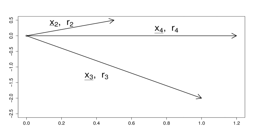
Now, let us shift the vectors ( x ¯ 1 , x ¯ 2 , x ¯ 3 , x ¯ 4 ) subscript ¯ 𝑥 1 subscript ¯ 𝑥 2 subscript ¯ 𝑥 3 subscript ¯ 𝑥 4 \left(\underline{x}_{1},\underline{x}_{2},\underline{x}_{3},\underline{x}_{4}\right) − x ¯ 1 subscript ¯ 𝑥 1 -\underline{x}_{1} ( x ¯ 2 − x ¯ 1 , x ¯ 3 − x ¯ 1 , x ¯ 4 − x ¯ 1 ) = ( y ¯ 2 , y ¯ 3 , y ¯ 4 ) subscript ¯ 𝑥 2 subscript ¯ 𝑥 1 subscript ¯ 𝑥 3 subscript ¯ 𝑥 1 subscript ¯ 𝑥 4 subscript ¯ 𝑥 1 subscript ¯ 𝑦 2 subscript ¯ 𝑦 3 subscript ¯ 𝑦 4 \left(\underline{x}_{2}-\underline{x}_{1},\underline{x}_{3}-\underline{x}_{1},\underline{x}_{4}-\underline{x}_{1}\right)=\left(\underline{y}_{2},\underline{y}_{3},\underline{y}_{4}\right) y ¯ 4 = | y ¯ 4 | n ¯ subscript ¯ 𝑦 4 subscript ¯ 𝑦 4 ¯ 𝑛 \underline{y}_{4}=\left|\underline{y}_{4}\right|\underline{n} n ¯ = ( 1 , 0 ) ¯ 𝑛 1 0 \underline{n}=\left(1,0\right) ( 0 ¯ , y ¯ 2 , y ¯ 3 , y ¯ 4 ) ¯ 0 subscript ¯ 𝑦 2 subscript ¯ 𝑦 3 subscript ¯ 𝑦 4 \left(\underline{0},\underline{y}_{2},\underline{y}_{3},\underline{y}_{4}\right) r 2 = | y ¯ 2 | subscript 𝑟 2 subscript ¯ 𝑦 2 r_{2}=\left|\underline{y}_{2}\right| r 3 = | y ¯ 3 | subscript 𝑟 3 subscript ¯ 𝑦 3 r_{3}=\left|\underline{y}_{3}\right| r 4 subscript 𝑟 4 r_{4} = | y ¯ 4 | absent subscript ¯ 𝑦 4 =\left|\underline{y}_{4}\right| ( r 2 , φ 2 ) subscript 𝑟 2 subscript 𝜑 2 \left(r_{2},\varphi_{2}\right) ( r 3 , φ 3 ) subscript 𝑟 3 subscript 𝜑 3 \left(r_{3},\varphi_{3}\right) ( ( r , φ ) 2 : 3 , r 4 ) = ( ( r 2 , φ 2 ) , ( r 3 , φ 3 ) , r 4 ) subscript 𝑟 𝜑 : 2 3 subscript 𝑟 4 subscript 𝑟 2 subscript 𝜑 2 subscript 𝑟 3 subscript 𝜑 3 subscript 𝑟 4 \left(\left(r,\varphi\right)_{2:3},r_{4}\right)=\left(\left(r_{2},\varphi_{2}\right),\left(r_{3},\varphi_{3}\right),r_{4}\right)
We use the invariance of the cumulants under the shift and rotation to obtain
Cum ( X ( x ¯ 1 ) , X ( x ¯ 2 ) , X ( x ¯ 3 ) , X ( x ¯ 4 ) ) = Cum ( X ( 0 ) , X ( x ¯ 2 − x ¯ 1 ) , X ( x ¯ 3 − x ¯ 1 ) , X ( x ¯ 4 − x ¯ 1 ) , ) = Cum ( X ( 0 ) , X ( g ( x ¯ 2 − x ¯ 1 ) ) , X ( g ( x ¯ 3 − x ¯ 1 ) ) , X ( g ( x ¯ 4 − x ¯ 1 ) ) ) \operatorname*{Cum}\left(X\left(\underline{x}_{1}\right),X\left(\underline{x}_{2}\right),X\left(\underline{x}_{3}\right),X\left(\underline{x}_{4}\right)\right)=\operatorname*{Cum}\left(X\left(0\right),X\left(\underline{x}_{2}-\underline{x}_{1}\right),X\left(\underline{x}_{3}-\underline{x}_{1}\right),X\left(\underline{x}_{4}-\underline{x}_{1}\right),\right)\\
=\operatorname*{Cum}\left(X\left(0\right),X\left(g\left(\underline{x}_{2}-\underline{x}_{1}\right)\right),X\left(g\left(\underline{x}_{3}-\underline{x}_{1}\right)\right),X\left(g\left(\underline{x}_{4}-\underline{x}_{1}\right)\right)\right)
where g 𝑔 g x ¯ 4 − x ¯ 1 subscript ¯ 𝑥 4 subscript ¯ 𝑥 1 \underline{x}_{4}-\underline{x}_{1} x 𝑥 x Cum ( X ( 0 ) , X ( x ¯ 2 ) , X ( x ¯ 3 ) , X ( r 4 n ¯ ) ) Cum 𝑋 0 𝑋 subscript ¯ 𝑥 2 𝑋 subscript ¯ 𝑥 3 𝑋 subscript 𝑟 4 ¯ 𝑛 \operatorname*{Cum}\left(X\left(0\right),X\left(\underline{x}_{2}\right),X\left(\underline{x}_{3}\right),X\left(r_{4}\underline{n}\right)\right) x ¯ 2 subscript ¯ 𝑥 2 \underline{x}_{2} x ¯ 3 subscript ¯ 𝑥 3 \underline{x}_{3} n ¯ = ( 1 , 0 ) ¯ 𝑛 1 0 \underline{n}=\left(1,0\right) X ( x ¯ ) 𝑋 ¯ 𝑥 X\left(\underline{x}\right) r 4 subscript 𝑟 4 r_{4} x ¯ 2 subscript ¯ 𝑥 2 \underline{x}_{2} x ¯ 3 subscript ¯ 𝑥 3 \underline{x}_{3} ( ( r , φ ) 2 : 3 , r 4 ) subscript 𝑟 𝜑 : 2 3 subscript 𝑟 4 \left(\left(r,\varphi\right)_{2:3},r_{4}\right) 1
𝒞 4 ( ( r 2 , φ 2 ) , ( r 3 , φ 3 ) , r 4 ) = Cum ( X ( x ¯ 1 ) , X ( x ¯ 2 ) , X ( r 3 n ¯ ) , X ( 0 ) ) , subscript 𝒞 4 subscript 𝑟 2 subscript 𝜑 2 subscript 𝑟 3 subscript 𝜑 3 subscript 𝑟 4 Cum 𝑋 subscript ¯ 𝑥 1 𝑋 subscript ¯ 𝑥 2 𝑋 subscript 𝑟 3 ¯ 𝑛 𝑋 0 \mathcal{C}_{4}\left(\left(r_{2},\varphi_{2}\right),\left(r_{3},\varphi_{3}\right),r_{4}\right)=\operatorname*{Cum}\left(X\left(\underline{x}_{1}\right),X\left(\underline{x}_{2}\right),X\left(r_{3}\underline{n}\right),X\left(0\right)\right),
and the trispectrum S 4 ( α 1 , ρ 2 : 4 , β 2 ) subscript 𝑆 4 subscript 𝛼 1 subscript 𝜌 : 2 4 subscript 𝛽 2 S_{4}\left(\alpha_{1},\rho_{2:4},\beta_{2}\right) ( α 1 , ρ 2 , ρ 3 , ρ 4 , β 2 ) subscript 𝛼 1 subscript 𝜌 2 subscript 𝜌 3 subscript 𝜌 4 subscript 𝛽 2 \left(\alpha_{1},\rho_{2},\rho_{3},\rho_{4},\beta_{2}\right) α 1 , β 2 ∈ ( 0 , π ) subscript 𝛼 1 subscript 𝛽 2
0 𝜋 \alpha_{1},\beta_{2}\in\left(0,\pi\right) 0 < ρ 2 , ρ 3 , ρ 4 0 subscript 𝜌 2 subscript 𝜌 3 subscript 𝜌 4
0<\rho_{2},\rho_{3},\rho_{4}
Let
𝒯 4 ( α 1 , ρ 2 : 4 , β 2 | ( r , φ ) 2 : 3 , r 4 ) subscript 𝒯 4 subscript 𝛼 1 subscript 𝜌 : 2 4 conditional subscript 𝛽 2 subscript 𝑟 𝜑 : 2 3 subscript 𝑟 4
\displaystyle\mathcal{T}_{4}\left(\left.\alpha_{1},\rho_{2:4},\beta_{2}\right|\left(r,\varphi\right)_{2:3},r_{4}\right)
= ∑ ℓ 2 , ℓ 3 = − ∞ ∞ e i ( ℓ 2 φ 2 + ℓ 3 φ 3 ) J ℓ 2 ( ρ 2 r 2 ) J ℓ 3 ( ρ 3 r 3 ) J ℓ 2 + ℓ 3 ( ρ 4 r 4 ) cos ( ℓ 2 α 1 ) cos ( ℓ 2 α 3 − ℓ 3 β 2 ) , absent superscript subscript subscript ℓ 2 subscript ℓ 3
superscript 𝑒 𝑖 subscript ℓ 2 subscript 𝜑 2 subscript ℓ 3 subscript 𝜑 3 subscript 𝐽 subscript ℓ 2 subscript 𝜌 2 subscript 𝑟 2 subscript 𝐽 subscript ℓ 3 subscript 𝜌 3 subscript 𝑟 3 subscript 𝐽 subscript ℓ 2 subscript ℓ 3 subscript 𝜌 4 subscript 𝑟 4 subscript ℓ 2 subscript 𝛼 1 subscript ℓ 2 subscript 𝛼 3 subscript ℓ 3 subscript 𝛽 2 \displaystyle=\sum_{\ell_{2},\ell_{3}=-\infty}^{\infty}e^{i\left(\ell_{2}\varphi_{2}+\ell_{3}\varphi_{3}\right)}J_{\ell_{2}}\left(\rho_{2}r_{2}\right)J_{\ell_{3}}\left(\rho_{3}r_{3}\right)J_{\ell_{2}+\ell_{3}}\left(\rho_{4}r_{4}\right)\cos\left(\ell_{2}\alpha_{1}\right)\cos\left(\ell_{2}\alpha_{3}-\ell_{3}\beta_{2}\right),
where the angle α 3 subscript 𝛼 3 \alpha_{3} ρ 2 , ρ 3 , ρ 4 subscript 𝜌 2 subscript 𝜌 3 subscript 𝜌 4
\rho_{2},\rho_{3},\rho_{4} ( ρ 2 2 + ρ 4 2 − ρ 3 2 ) / ( 2 ρ 2 ρ 4 ) = cos α 3 superscript subscript 𝜌 2 2 superscript subscript 𝜌 4 2 superscript subscript 𝜌 3 2 2 subscript 𝜌 2 subscript 𝜌 4 subscript 𝛼 3 \left(\rho_{2}^{2}+\rho_{4}^{2}-\rho_{3}^{2}\right)/\left(2\rho_{2}\rho_{4}\right)=\cos\alpha_{3} 3
Theorem 1 .
Let X ( x ¯ ) 𝑋 ¯ 𝑥 X\left(\underline{x}\right)
𝒞 4 ( ( r , φ ) 2 : 3 , r 4 ) subscript 𝒞 4 subscript 𝑟 𝜑 : 2 3 subscript 𝑟 4 \displaystyle\mathcal{C}_{4}\left(\left(r,\varphi\right)_{2:3},r_{4}\right) = 4 ∭ 0 ∞ ∬ 0 π 𝒯 4 ( α 1 , ρ 2 : 4 , β 2 | ( r , φ ) 2 : 3 , r 4 ) absent 4 superscript subscript triple-integral 0 superscript subscript double-integral 0 𝜋 subscript 𝒯 4 subscript 𝛼 1 subscript 𝜌 : 2 4 conditional subscript 𝛽 2 subscript 𝑟 𝜑 : 2 3 subscript 𝑟 4
\displaystyle=4\iiint\limits_{0}^{\infty}\iint_{0}^{\pi}\mathcal{T}_{4}\left(\left.\alpha_{1},\rho_{2:4},\beta_{2}\right|\left(r,\varphi\right)_{2:3},r_{4}\right)
× S 4 ( α 1 , ρ 2 : 4 , β 2 ) ∏ k = 2 4 ρ k d ρ k d α 1 d β 2 , absent subscript 𝑆 4 subscript 𝛼 1 subscript 𝜌 : 2 4 subscript 𝛽 2 superscript subscript product 𝑘 2 4 subscript 𝜌 𝑘 𝑑 subscript 𝜌 𝑘 𝑑 subscript 𝛼 1 𝑑 subscript 𝛽 2 \displaystyle\times S_{4}\left(\alpha_{1},\rho_{2:4},\beta_{2}\right){\textstyle\prod\limits_{k=2}^{4}}\rho_{k}d\rho_{k}d\alpha_{1}d\beta_{2},
In return
S 4 ( α 1 , ρ 2 : 4 , β 2 ) subscript 𝑆 4 subscript 𝛼 1 subscript 𝜌 : 2 4 subscript 𝛽 2 \displaystyle S_{4}\left(\alpha_{1},\rho_{2:4},\beta_{2}\right) = 1 ( 2 π ) 4 ∭ 0 ∞ ∬ 0 2 π 𝒯 4 ( α 1 , ρ 2 : 4 , β 2 | ( r , φ ) 2 : 3 , r 4 ) absent 1 superscript 2 𝜋 4 superscript subscript triple-integral 0 superscript subscript double-integral 0 2 𝜋 subscript 𝒯 4 subscript 𝛼 1 subscript 𝜌 : 2 4 conditional subscript 𝛽 2 subscript 𝑟 𝜑 : 2 3 subscript 𝑟 4
\displaystyle=\frac{1}{\left(2\pi\right)^{4}}\iiint\limits_{0}^{\infty}\iint_{0}^{2\pi}\mathcal{T}_{4}\left(\left.\alpha_{1},\rho_{2:4},\beta_{2}\right|\left(r,\varphi\right)_{2:3},r_{4}\right)
(2.1) × 𝒞 4 ( ( r , φ ) 2 : 3 , r 4 ) ∏ k = 2 4 r k d r k d φ 2 d φ 3 , absent subscript 𝒞 4 subscript 𝑟 𝜑 : 2 3 subscript 𝑟 4 superscript subscript product 𝑘 2 4 subscript 𝑟 𝑘 𝑑 subscript 𝑟 𝑘 𝑑 subscript 𝜑 2 𝑑 subscript 𝜑 3 \displaystyle\times\mathcal{C}_{4}\left(\left(r,\varphi\right)_{2:3},r_{4}\right){\textstyle\prod\limits_{k=2}^{4}}r_{k}dr_{k}d\varphi_{2}d\varphi_{3},
unless the integrals exist.
Proof.
We apply the series representation (1.1 X ( x ¯ ) 𝑋 ¯ 𝑥 X\left(\underline{x}\right) n ¯ = ( − 1 , 0 ) ¯ 𝑛 1 0 \underline{n}=\left(-1,0\right)
(2.2) X ( r n ¯ ) 𝑋 𝑟 ¯ 𝑛 \displaystyle X\left(r\underline{n}\right) = ∑ ℓ = − ∞ ∞ ∫ 0 ∞ J ℓ ( ρ r ) Z ℓ ( ρ d ρ ) , absent superscript subscript ℓ superscript subscript 0 subscript 𝐽 ℓ 𝜌 𝑟 subscript 𝑍 ℓ 𝜌 𝑑 𝜌 \displaystyle=\sum_{\ell=-\infty}^{\infty}\int_{0}^{\infty}J_{\ell}\left(\rho r\right)Z_{\ell}\left(\rho d\rho\right),
(2.3) X ( 0 ¯ ) 𝑋 ¯ 0 \displaystyle X\left(\underline{0}\right) = ∫ ℝ 2 Z ( d ω ¯ ) absent subscript superscript ℝ 2 𝑍 𝑑 ¯ 𝜔 \displaystyle=\int_{\mathbb{R}^{2}}Z\left(d\underline{\omega}\right)
= ∫ 0 ∞ Z 0 ( ρ d ρ ) . absent superscript subscript 0 subscript 𝑍 0 𝜌 𝑑 𝜌 \displaystyle=\int_{0}^{\infty}Z_{0}\left(\rho d\rho\right).
We obtain
Cum ( X ( 0 ) , X ( x ¯ 2 ) , X ( x ¯ 3 ) , X ( r 4 n ¯ ) ) = ∑ ℓ 2 , ℓ 3 , ℓ 4 = − ∞ ∞ e i ( ℓ 2 φ 2 + ℓ 3 φ 3 ) × ⨌ 0 ∞ J ℓ 2 ( ρ 2 r 2 ) J ℓ 3 ( ρ 3 r 3 ) J ℓ 4 ( ρ 4 r 4 ) Cum ( Z 0 ( ρ 1 d ρ 1 ) , Z ℓ 2 ( ρ 2 d ρ 2 ) , Z ℓ 3 ( ρ 3 d ρ 3 ) , Z ℓ 4 ( ρ 4 d ρ 4 ) ) = ∑ ℓ 2 , ℓ 3 = − ∞ ∞ e i ( ℓ 2 φ 2 + ℓ 3 φ 3 ) ⨌ 0 ∞ J ℓ 2 ( ρ 2 r 2 ) J ℓ 3 ( ρ 3 r 3 ) J − ( ℓ 2 + ℓ 3 ) ( ρ 4 r 4 ) × Cum ( Z 0 ( ρ 1 d ρ 1 ) , Z ℓ 2 ( ρ 2 d ρ 2 ) , Z ℓ 3 ( ρ 3 d ρ 3 ) , Z − ( ℓ 2 + ℓ 3 ) ( ρ 4 d ρ 4 ) ) = ∑ ℓ 2 , ℓ 3 = − ∞ ∞ e i ( ℓ 2 φ 2 + ℓ 3 φ 3 ) ⨌ 0 ∞ J ℓ 2 ( ρ 2 r 2 ) J ℓ 3 ( ρ 3 r 3 ) J ℓ 2 + ℓ 3 ( ρ 4 r 4 ) × ( − 1 ) ℓ 2 + ℓ 3 Cum ( Z 0 ( ρ 1 d ρ 1 ) , Z ℓ 2 ( ρ 2 d ρ 2 ) , Z ℓ 3 ( ρ 3 d ρ 3 ) , Z − ( ℓ 2 + ℓ 3 ) ( ρ 4 d ρ 4 ) ) , Cum 𝑋 0 𝑋 subscript ¯ 𝑥 2 𝑋 subscript ¯ 𝑥 3 𝑋 subscript 𝑟 4 ¯ 𝑛 superscript subscript subscript ℓ 2 subscript ℓ 3 subscript ℓ 4
superscript 𝑒 𝑖 subscript ℓ 2 subscript 𝜑 2 subscript ℓ 3 subscript 𝜑 3 superscript subscript quadruple-integral 0 subscript 𝐽 subscript ℓ 2 subscript 𝜌 2 subscript 𝑟 2 subscript 𝐽 subscript ℓ 3 subscript 𝜌 3 subscript 𝑟 3 subscript 𝐽 subscript ℓ 4 subscript 𝜌 4 subscript 𝑟 4 Cum subscript 𝑍 0 subscript 𝜌 1 𝑑 subscript 𝜌 1 subscript 𝑍 subscript ℓ 2 subscript 𝜌 2 𝑑 subscript 𝜌 2 subscript 𝑍 subscript ℓ 3 subscript 𝜌 3 𝑑 subscript 𝜌 3 subscript 𝑍 subscript ℓ 4 subscript 𝜌 4 𝑑 subscript 𝜌 4 superscript subscript subscript ℓ 2 subscript ℓ 3
superscript 𝑒 𝑖 subscript ℓ 2 subscript 𝜑 2 subscript ℓ 3 subscript 𝜑 3 superscript subscript quadruple-integral 0 subscript 𝐽 subscript ℓ 2 subscript 𝜌 2 subscript 𝑟 2 subscript 𝐽 subscript ℓ 3 subscript 𝜌 3 subscript 𝑟 3 subscript 𝐽 subscript ℓ 2 subscript ℓ 3 subscript 𝜌 4 subscript 𝑟 4 Cum subscript 𝑍 0 subscript 𝜌 1 𝑑 subscript 𝜌 1 subscript 𝑍 subscript ℓ 2 subscript 𝜌 2 𝑑 subscript 𝜌 2 subscript 𝑍 subscript ℓ 3 subscript 𝜌 3 𝑑 subscript 𝜌 3 subscript 𝑍 subscript ℓ 2 subscript ℓ 3 subscript 𝜌 4 𝑑 subscript 𝜌 4 superscript subscript subscript ℓ 2 subscript ℓ 3
superscript 𝑒 𝑖 subscript ℓ 2 subscript 𝜑 2 subscript ℓ 3 subscript 𝜑 3 superscript subscript quadruple-integral 0 subscript 𝐽 subscript ℓ 2 subscript 𝜌 2 subscript 𝑟 2 subscript 𝐽 subscript ℓ 3 subscript 𝜌 3 subscript 𝑟 3 subscript 𝐽 subscript ℓ 2 subscript ℓ 3 subscript 𝜌 4 subscript 𝑟 4 superscript 1 subscript ℓ 2 subscript ℓ 3 Cum subscript 𝑍 0 subscript 𝜌 1 𝑑 subscript 𝜌 1 subscript 𝑍 subscript ℓ 2 subscript 𝜌 2 𝑑 subscript 𝜌 2 subscript 𝑍 subscript ℓ 3 subscript 𝜌 3 𝑑 subscript 𝜌 3 subscript 𝑍 subscript ℓ 2 subscript ℓ 3 subscript 𝜌 4 𝑑 subscript 𝜌 4 \operatorname*{Cum}\left(X\left(0\right),X\left(\underline{x}_{2}\right),X\left(\underline{x}_{3}\right),X\left(r_{4}\underline{n}\right)\right)=\sum_{\ell_{2},\ell_{3},\ell_{4}=-\infty}^{\infty}e^{i\left(\ell_{2}\varphi_{2}+\ell_{3}\varphi_{3}\right)}\\
\times\iiiint\limits_{0}^{\infty}J_{\ell_{2}}\left(\rho_{2}r_{2}\right)J_{\ell_{3}}\left(\rho_{3}r_{3}\right)J_{\ell_{4}}\left(\rho_{4}r_{4}\right)\operatorname*{Cum}\left(Z_{0}\left(\rho_{1}d\rho_{1}\right),Z_{\ell_{2}}\left(\rho_{2}d\rho_{2}\right),Z_{\ell_{3}}\left(\rho_{3}d\rho_{3}\right),Z_{\ell_{4}}\left(\rho_{4}d\rho_{4}\right)\right)\\
=\sum_{\ell_{2},\ell_{3}=-\infty}^{\infty}e^{i\left(\ell_{2}\varphi_{2}+\ell_{3}\varphi_{3}\right)}\iiiint\limits_{0}^{\infty}J_{\ell_{2}}\left(\rho_{2}r_{2}\right)J_{\ell_{3}}\left(\rho_{3}r_{3}\right)J_{-\left(\ell_{2}+\ell_{3}\right)}\left(\rho_{4}r_{4}\right)\\
\times\operatorname*{Cum}\left(Z_{0}\left(\rho_{1}d\rho_{1}\right),Z_{\ell_{2}}\left(\rho_{2}d\rho_{2}\right),Z_{\ell_{3}}\left(\rho_{3}d\rho_{3}\right),Z_{-\left(\ell_{2}+\ell_{3}\right)}\left(\rho_{4}d\rho_{4}\right)\right)\\
=\sum_{\ell_{2},\ell_{3}=-\infty}^{\infty}e^{i\left(\ell_{2}\varphi_{2}+\ell_{3}\varphi_{3}\right)}\iiiint\limits_{0}^{\infty}J_{\ell_{2}}\left(\rho_{2}r_{2}\right)J_{\ell_{3}}\left(\rho_{3}r_{3}\right)J_{\ell_{2}+\ell_{3}}\left(\rho_{4}r_{4}\right)\\
\times\left(-1\right)^{\ell_{2}+\ell_{3}}\operatorname*{Cum}\left(Z_{0}\left(\rho_{1}d\rho_{1}\right),Z_{\ell_{2}}\left(\rho_{2}d\rho_{2}\right),Z_{\ell_{3}}\left(\rho_{3}d\rho_{3}\right),Z_{-\left(\ell_{2}+\ell_{3}\right)}\left(\rho_{4}d\rho_{4}\right)\right),
in polar coordinates. The fourth order cumulant of the stochastic spectral
measure Z ( d ω ¯ ) 𝑍 𝑑 ¯ 𝜔 Z\left(d\underline{\omega}\right) X ( x ¯ ) 𝑋 ¯ 𝑥 X\left(\underline{x}\right)
Cum ( Z ( d ω ¯ 1 ) , Z ( d ω ¯ 2 ) , Z ( d ω ¯ 3 ) , Z ( d ω ¯ 4 ) ) = δ ( Σ 1 4 ω ¯ k ) S 4 ( ω ¯ 1 : 4 ) ∏ k = 1 4 d ω ¯ k , Cum 𝑍 𝑑 subscript ¯ 𝜔 1 𝑍 𝑑 subscript ¯ 𝜔 2 𝑍 𝑑 subscript ¯ 𝜔 3 𝑍 𝑑 subscript ¯ 𝜔 4 𝛿 superscript subscript Σ 1 4 subscript ¯ 𝜔 𝑘 subscript 𝑆 4 subscript ¯ 𝜔 : 1 4 superscript subscript product 𝑘 1 4 𝑑 subscript ¯ 𝜔 𝑘 \operatorname*{Cum}\left(Z\left(d\underline{\omega}_{1}\right),Z\left(d\underline{\omega}_{2}\right),Z\left(d\underline{\omega}_{3}\right),Z\left(d\underline{\omega}_{4}\right)\right)=\delta\left(\Sigma_{1}^{4}\underline{\omega}_{k}\right)S_{4}\left(\underline{\omega}_{1:4}\right){\textstyle\prod\limits_{k=1}^{4}}d\underline{\omega}_{k},
and the stochastic spectral measures Z ℓ ( ρ d ρ ) subscript 𝑍 ℓ 𝜌 𝑑 𝜌 Z_{\ell}\left(\rho d\rho\right) Z ( d ω ¯ ) 𝑍 𝑑 ¯ 𝜔 Z\left(d\underline{\omega}\right) 1.2
Cum ( Z 0 ( ρ 1 d ρ 1 ) , Z ℓ 2 ( ρ 2 d ρ 2 ) , Z ℓ 3 ( ρ 3 d ρ 3 ) , Z − ( ℓ 2 + ℓ 3 ) ( ρ 4 d ρ 4 ) ) Cum subscript 𝑍 0 subscript 𝜌 1 𝑑 subscript 𝜌 1 subscript 𝑍 subscript ℓ 2 subscript 𝜌 2 𝑑 subscript 𝜌 2 subscript 𝑍 subscript ℓ 3 subscript 𝜌 3 𝑑 subscript 𝜌 3 subscript 𝑍 subscript ℓ 2 subscript ℓ 3 subscript 𝜌 4 𝑑 subscript 𝜌 4 \displaystyle\operatorname*{Cum}\left(Z_{0}\left(\rho_{1}d\rho_{1}\right),Z_{\ell_{2}}\left(\rho_{2}d\rho_{2}\right),Z_{\ell_{3}}\left(\rho_{3}d\rho_{3}\right),Z_{-\left(\ell_{2}+\ell_{3}\right)}\left(\rho_{4}d\rho_{4}\right)\right)
(2.4) = 4 ( − 1 ) ℓ 2 + ℓ 3 ∫ 0 π δ ( △ | ρ 1 , ρ 2 , κ ) ρ 1 κ sin α 2 cos ( ℓ 2 α 1 ) cos ( ℓ 2 α 3 + ℓ 3 β 2 ) S 4 ( α 1 , ρ 2 : 4 , β 2 ) 𝑑 β 2 ∏ k = 1 4 ρ k d ρ k \displaystyle=4\left(-1\right)^{\ell_{2}+\ell_{3}}\int_{0}^{\pi}\frac{\delta\left(\bigtriangleup|\rho_{1},\rho_{2},\kappa\right)}{\rho_{1}\kappa\sin\alpha_{2}}\cos\left(\ell_{2}\alpha_{1}\right)\cos\left(\ell_{2}\alpha_{3}+\ell_{3}\beta_{2}\right)S_{4}\left(\alpha_{1},\rho_{2:4},\beta_{2}\right)d\beta_{2}{\textstyle\prod\limits_{k=1}^{4}}\rho_{k}d\rho_{k}
where ω ¯ ^ k = ω ¯ k / | ω ¯ k | = ( cos η k , sin η k ) subscript ¯ ^ 𝜔 𝑘 subscript ¯ 𝜔 𝑘 subscript ¯ 𝜔 𝑘 subscript 𝜂 𝑘 subscript 𝜂 𝑘 \underline{\widehat{\omega}}_{k}=\underline{\omega}_{k}/\left|\underline{\omega}_{k}\right|=\left(\cos\eta_{k},\sin\eta_{k}\right) η k subscript 𝜂 𝑘 \eta_{k} Cum ( X ( 0 ) , X ( x ¯ 2 ) , X ( x ¯ 3 ) , X ( r 4 n ¯ ) ) Cum 𝑋 0 𝑋 subscript ¯ 𝑥 2 𝑋 subscript ¯ 𝑥 3 𝑋 subscript 𝑟 4 ¯ 𝑛 \operatorname*{Cum}\left(X\left(0\right),X\left(\underline{x}_{2}\right),X\left(\underline{x}_{3}\right),X\left(r_{4}\underline{n}\right)\right) ( ( r , φ ) 2 : 3 , r 4 ) subscript 𝑟 𝜑 : 2 3 subscript 𝑟 4 \left(\left(r,\varphi\right)_{2:3},r_{4}\right) 1
Figure 1. Locations on the plane
The function 𝒞 4 ( ( ( r , φ ) 2 : 3 , r 4 ) ) subscript 𝒞 4 subscript 𝑟 𝜑 : 2 3 subscript 𝑟 4 \mathcal{C}_{4}\left(\left(\left(r,\varphi\right)_{2:3},r_{4}\right)\right)
Cum ( X ( 0 ) , X ( x ¯ 2 ) , X ( x ¯ 3 ) , X ( r 4 n ¯ ) ) = 4 ∑ ℓ 2 , ℓ 3 = − ∞ ∞ e i ( ℓ 2 φ 2 + ℓ 3 φ 3 ) ⨌ 0 ∞ J ℓ 2 ( ρ 2 r 2 ) J ℓ 3 ( ρ 3 r 3 ) J ℓ 2 + ℓ 3 ( ρ 4 r 4 ) × δ ( △ | ρ 1 , ρ 2 , κ ) ρ 2 κ sin α 1 e − i ℓ 2 ( α 1 − α 3 ) − i ℓ 3 β 2 S 4 ( α 1 , ρ 2 : 4 , β 2 ) d β 2 ∏ k = 1 4 ρ k d ρ k = 4 ∑ ℓ 2 , ℓ 3 = − ∞ ∞ e i ( ℓ 2 φ 2 + ℓ 3 φ 3 ) ∭ 0 ∞ J ℓ 2 ( ρ 2 r 2 ) J ℓ 3 ( ρ 3 r 3 ) J ℓ 2 + ℓ 3 ( ρ 4 r 4 ) ∬ 0 π cos ( ℓ 2 α 1 ) cos ( ℓ 2 α 3 + ℓ 3 β 2 ) S 4 ( α 1 , ρ 2 : 4 , β 2 ) 𝑑 α 1 𝑑 β 2 ∏ k = 2 4 ρ k d ρ k , \operatorname*{Cum}\left(X\left(0\right),X\left(\underline{x}_{2}\right),X\left(\underline{x}_{3}\right),X\left(r_{4}\underline{n}\right)\right)\\
=4\sum_{\ell_{2},\ell_{3}=-\infty}^{\infty}e^{i\left(\ell_{2}\varphi_{2}+\ell_{3}\varphi_{3}\right)}\iiiint\limits_{0}^{\infty}J_{\ell_{2}}\left(\rho_{2}r_{2}\right)J_{\ell_{3}}\left(\rho_{3}r_{3}\right)J_{\ell_{2}+\ell_{3}}\left(\rho_{4}r_{4}\right)\\
\times\frac{\delta\left(\bigtriangleup|\rho_{1},\rho_{2},\kappa\right)}{\rho_{2}\kappa\sin\alpha_{1}}e^{-i\ell_{2}\left(\alpha_{1}-\alpha_{3}\right)-i\ell_{3}\beta_{2}\ }S_{4}\left(\alpha_{1},\rho_{2:4},\beta_{2}\right)d\beta_{2}{\textstyle\prod\limits_{k=1}^{4}}\rho_{k}d\rho_{k}\\
=4\sum_{\ell_{2},\ell_{3}=-\infty}^{\infty}e^{i\left(\ell_{2}\varphi_{2}+\ell_{3}\varphi_{3}\right)}\iiint\limits_{0}^{\infty}J_{\ell_{2}}\left(\rho_{2}r_{2}\right)J_{\ell_{3}}\left(\rho_{3}r_{3}\right)J_{\ell_{2}+\ell_{3}}\left(\rho_{4}r_{4}\right)\\
\iint\limits_{0}^{\pi}\cos\left(\ell_{2}\alpha_{1}\right)\cos\left(\ell_{2}\alpha_{3}+\ell_{3}\beta_{2}\right)S_{4}\left(\alpha_{1},\rho_{2:4},\beta_{2}\right)d\alpha_{1}d\beta_{2}{\textstyle\prod\limits_{k=2}^{4}}\rho_{k}d\rho_{k},
ρ 1 d ρ 1 = κ ρ 2 sin ( α 1 ) d α 1 subscript 𝜌 1 𝑑 subscript 𝜌 1 𝜅 subscript 𝜌 2 subscript 𝛼 1 𝑑 subscript 𝛼 1 \rho_{1}d\rho_{1}=\kappa\rho_{2}\sin\left(\alpha_{1}\right)d\alpha_{1} κ = ρ 3 2 + ρ 4 2 − 2 ρ 3 ρ 4 cos β 2 𝜅 superscript subscript 𝜌 3 2 superscript subscript 𝜌 4 2 2 subscript 𝜌 3 subscript 𝜌 4 subscript 𝛽 2 \kappa=\sqrt{\rho_{3}^{2}+\rho_{4}^{2}-2\rho_{3}\rho_{4}\cos\beta_{2}} α 2 = arccos [ ( ρ 3 2 − ρ 4 2 − κ 2 ) / 2 κ ρ 4 ] subscript 𝛼 2 superscript subscript 𝜌 3 2 superscript subscript 𝜌 4 2 superscript 𝜅 2 2 𝜅 subscript 𝜌 4 \alpha_{2}=\arccos\left[\left(\rho_{3}^{2}-\rho_{4}^{2}-\kappa^{2}\right)/2\kappa\rho_{4}\right] α 3 subscript 𝛼 3 \alpha_{3} ρ 3 subscript 𝜌 3 \rho_{3} ρ 4 subscript 𝜌 4 \rho_{4} β 2 subscript 𝛽 2 \beta_{2} 2.1
∬ 0 2 π ∭ 0 ∞ 𝒯 4 ( α 1 , ρ 2 : 4 , β 2 | ( r , φ ) 2 : 3 , r 4 ) 𝒞 4 ( ( r , φ ) 2 : 3 , r 4 ) 𝑑 φ 2 𝑑 φ 3 ∏ k = 2 4 r k d r k superscript subscript double-integral 0 2 𝜋 superscript subscript triple-integral 0 subscript 𝒯 4 subscript 𝛼 1 subscript 𝜌 : 2 4 conditional subscript 𝛽 2 subscript 𝑟 𝜑 : 2 3 subscript 𝑟 4
subscript 𝒞 4 subscript 𝑟 𝜑 : 2 3 subscript 𝑟 4 differential-d subscript 𝜑 2 differential-d subscript 𝜑 3 superscript subscript product 𝑘 2 4 subscript 𝑟 𝑘 𝑑 subscript 𝑟 𝑘 \displaystyle\iint\limits_{0}^{2\pi}\iiint\limits_{0}^{\infty}\mathcal{T}_{4}\left(\left.\alpha_{1},\rho_{2:4},\beta_{2}\right|\left(r,\varphi\right)_{2:3},r_{4}\right)\mathcal{C}_{4}\left(\left(r,\varphi\right)_{2:3},r_{4}\right)d\varphi_{2}d\varphi_{3}{\textstyle\prod\limits_{k=2}^{4}}r_{k}dr_{k}
= 4 ∬ 0 2 π ∭ 0 ∞ 𝒯 4 ( α 1 , ρ 2 : 4 , β 2 | ( r , φ ) 2 : 3 , r 4 ) absent 4 superscript subscript double-integral 0 2 𝜋 superscript subscript triple-integral 0 subscript 𝒯 4 subscript 𝛼 1 subscript 𝜌 : 2 4 conditional subscript 𝛽 2 subscript 𝑟 𝜑 : 2 3 subscript 𝑟 4
\displaystyle=4\iint\limits_{0}^{2\pi}\iiint\limits_{0}^{\infty}\mathcal{T}_{4}\left(\left.\alpha_{1},\rho_{2:4},\beta_{2}\right|\left(r,\varphi\right)_{2:3},r_{4}\right)
∬ 0 2 π ∭ 0 ∞ 𝒯 4 ( α 1 ′ , ρ 2 : 4 ′ , β 2 ′ | ( r , φ ) 2 : 3 , r 4 ) S 4 ( α 1 ′ , ρ 2 : 4 ′ , β 2 ′ ) 𝑑 α 1 ′ 𝑑 β 2 ′ ∏ k = 2 4 ρ k ′ d ρ k ′ d φ 2 d φ 3 ∏ k = 2 4 r k d r k superscript subscript double-integral 0 2 𝜋 superscript subscript triple-integral 0 subscript 𝒯 4 superscript subscript 𝛼 1 ′ superscript subscript 𝜌 : 2 4 ′ conditional superscript subscript 𝛽 2 ′ subscript 𝑟 𝜑 : 2 3 subscript 𝑟 4
subscript 𝑆 4 superscript subscript 𝛼 1 ′ superscript subscript 𝜌 : 2 4 ′ superscript subscript 𝛽 2 ′ differential-d superscript subscript 𝛼 1 ′ differential-d superscript subscript 𝛽 2 ′ superscript subscript product 𝑘 2 4 superscript subscript 𝜌 𝑘 ′ 𝑑 superscript subscript 𝜌 𝑘 ′ 𝑑 subscript 𝜑 2 𝑑 subscript 𝜑 3 superscript subscript product 𝑘 2 4 subscript 𝑟 𝑘 𝑑 subscript 𝑟 𝑘 \displaystyle\iint\limits_{0}^{2\pi}\iiint\limits_{0}^{\infty}\mathcal{T}_{4}\left(\left.\alpha_{1}^{\prime},\rho_{2:4}^{\prime},\beta_{2}^{\prime}\right|\left(r,\varphi\right)_{2:3},r_{4}\right)S_{4}\left(\alpha_{1}^{\prime},\rho_{2:4}^{\prime},\beta_{2}^{\prime}\right)d\alpha_{1}^{\prime}d\beta_{2}^{\prime}{\textstyle\prod\limits_{k=2}^{4}}\rho_{k}^{\prime}d\rho_{k}^{\prime}d\varphi_{2}d\varphi_{3}{\textstyle\prod\limits_{k=2}^{4}}r_{k}dr_{k}
= 4 ( 2 π ) 2 ∑ ℓ 2 , ℓ 3 = − ∞ ∞ ∭ 0 ∞ ∭ 0 ∞ J ℓ 2 ( ρ 2 ′ r 2 ) J ℓ 3 ( ρ 3 ′ r 3 ) J ℓ 2 + ℓ 3 ( ρ 4 ′ r 4 ) J ℓ 2 ( ρ 2 r 2 ) J ℓ 3 ( ρ 3 r 3 ) J ℓ 2 + ℓ 3 ( ρ 4 r 4 ) ∏ k = 2 4 r k d r k absent 4 superscript 2 𝜋 2 superscript subscript subscript ℓ 2 subscript ℓ 3
superscript subscript triple-integral 0 superscript subscript triple-integral 0 subscript 𝐽 subscript ℓ 2 superscript subscript 𝜌 2 ′ subscript 𝑟 2 subscript 𝐽 subscript ℓ 3 superscript subscript 𝜌 3 ′ subscript 𝑟 3 subscript 𝐽 subscript ℓ 2 subscript ℓ 3 superscript subscript 𝜌 4 ′ subscript 𝑟 4 subscript 𝐽 subscript ℓ 2 subscript 𝜌 2 subscript 𝑟 2 subscript 𝐽 subscript ℓ 3 subscript 𝜌 3 subscript 𝑟 3 subscript 𝐽 subscript ℓ 2 subscript ℓ 3 subscript 𝜌 4 subscript 𝑟 4 superscript subscript product 𝑘 2 4 subscript 𝑟 𝑘 𝑑 subscript 𝑟 𝑘 \displaystyle=4\left(2\pi\right)^{2}\sum_{\ell_{2},\ell_{3}=-\infty}^{\infty}\iiint\limits_{0}^{\infty}\iiint\limits_{0}^{\infty}J_{\ell_{2}}\left(\rho_{2}^{\prime}r_{2}\right)J_{\ell_{3}}\left(\rho_{3}^{\prime}r_{3}\right)J_{\ell_{2}+\ell_{3}}\left(\rho_{4}^{\prime}r_{4}\right)J_{\ell_{2}}\left(\rho_{2}r_{2}\right)J_{\ell_{3}}\left(\rho_{3}r_{3}\right)J_{\ell_{2}+\ell_{3}}\left(\rho_{4}r_{4}\right){\textstyle\prod\limits_{k=2}^{4}}r_{k}dr_{k}
× ∬ 0 π cos ( ℓ 2 α 1 ′ ) cos ( ℓ 2 α 3 ′ + ℓ 3 β 2 ′ ) cos ( ℓ 2 α 1 ) cos ( ℓ 2 α 3 + ℓ 3 β 2 ) S 4 ( α 1 ′ , ρ 2 : 4 ′ , β 2 ′ ) d α 1 ′ d β 2 ′ ∏ k = 2 4 ρ k ′ d ρ k ′ \displaystyle\times\iint\limits_{0}^{\pi}\cos\left(\ell_{2}\alpha_{1}^{\prime}\right)\cos\left(\ell_{2}\alpha_{3}^{\prime}+\ell_{3}\beta_{2}^{\prime}\right)\cos\left(\ell_{2}\alpha_{1}\right)\cos\left(\ell_{2}\alpha_{3}+\ell_{3}\beta_{2}\right)S_{4}\left(\alpha_{1}^{\prime},\rho_{2:4}^{\prime},\beta_{2}^{\prime}\right)d\alpha_{1}^{\prime}d\beta_{2}^{\prime}{\textstyle\prod\limits_{k=2}^{4}}\rho_{k}^{\prime}d\rho_{k}^{\prime}
= 4 ( 2 π ) 2 ∬ 0 π ∑ ℓ 2 , ℓ 3 = − ∞ ∞ cos ( ℓ 2 α 1 ′ ) cos ( ℓ 2 α 3 ′ + ℓ 3 β 2 ′ ) cos ( ℓ 2 α 1 ) cos ( ℓ 2 α 3 + ℓ 3 β 2 ) S 4 ( α 1 ′ , ρ 2 : 4 , β 2 ′ ) d α 1 ′ d β 2 ′ absent 4 superscript 2 𝜋 2 superscript subscript double-integral 0 𝜋 superscript subscript subscript ℓ 2 subscript ℓ 3
subscript ℓ 2 superscript subscript 𝛼 1 ′ subscript ℓ 2 superscript subscript 𝛼 3 ′ subscript ℓ 3 superscript subscript 𝛽 2 ′ subscript ℓ 2 subscript 𝛼 1 subscript ℓ 2 subscript 𝛼 3 subscript ℓ 3 subscript 𝛽 2 subscript 𝑆 4 superscript subscript 𝛼 1 ′ subscript 𝜌 : 2 4 superscript subscript 𝛽 2 ′ 𝑑 superscript subscript 𝛼 1 ′ 𝑑 superscript subscript 𝛽 2 ′ \displaystyle=4\left(2\pi\right)^{2}\iint\limits_{0}^{\pi}\sum_{\ell_{2},\ell_{3}=-\infty}^{\infty}\cos\left(\ell_{2}\alpha_{1}^{\prime}\right)\cos\left(\ell_{2}\alpha_{3}^{\prime}+\ell_{3}\beta_{2}^{\prime}\right)\cos\left(\ell_{2}\alpha_{1}\right)\cos\left(\ell_{2}\alpha_{3}+\ell_{3}\beta_{2}\right)S_{4}\left(\alpha_{1}^{\prime},\rho_{2:4},\beta_{2}^{\prime}\right)d\alpha_{1}^{\prime}d\beta_{2}^{\prime}
= ( 2 π ) 4 S 4 ( α 1 , ρ 2 : 4 , β 2 ) , absent superscript 2 𝜋 4 subscript 𝑆 4 subscript 𝛼 1 subscript 𝜌 : 2 4 subscript 𝛽 2 \displaystyle=\left(2\pi\right)^{4}S_{4}\left(\alpha_{1},\rho_{2:4},\beta_{2}\right),
To show the last equality, one can turn cosine to exponential and get the
result, since both β 2 subscript 𝛽 2 \beta_{2} β 2 ′ superscript subscript 𝛽 2 ′ \beta_{2}^{\prime} α 3 subscript 𝛼 3 \alpha_{3}\ α 3 ′ superscript subscript 𝛼 3 ′ \alpha_{3}^{\prime} β 2 = β 2 ′ subscript 𝛽 2 superscript subscript 𝛽 2 ′ \beta_{2}=\beta_{2}^{\prime} α 3 = α 3 ′ subscript 𝛼 3 superscript subscript 𝛼 3 ′ \alpha_{3}=\alpha_{3}^{\prime} α 1 = α 1 ′ subscript 𝛼 1 superscript subscript 𝛼 1 ′ \alpha_{1}=\alpha_{1}^{\prime}
3. Expression for Higher Order Spectra
The Theorem 1 ρ 2 : p = ( ρ 2 , … , ρ p ) subscript 𝜌 : 2 𝑝 subscript 𝜌 2 … subscript 𝜌 𝑝 \rho_{2:p}=\left(\rho_{2},\ldots,\rho_{p}\right) β 1 : p − 3 , 2 = ( β 1 , 2 , … , β p − 3 , 2 ) subscript 𝛽 : 1 𝑝 3 2
subscript 𝛽 1 2
… subscript 𝛽 𝑝 3 2
\beta_{1:p-3,2}=\left(\beta_{1,2},\ldots,\beta_{p-3,2}\right) ( r , φ ) 2 : p − 1 , = ( ( r 2 , φ 2 ) , … , ( r p − 1 , φ p − 1 ) ) \left(r,\varphi\right)_{2:p-1},=\left(\left(r_{2},\varphi_{2}\right),\ldots,\left(r_{p-1},\varphi_{p-1}\right)\right)
𝒯 p ( α 1 , ρ 2 : p , β 1 : p − 3 , 2 | ( r , φ ) 2 : p − 1 , r p ) = ∑ ℓ 2 , … , ℓ p − 1 = − ∞ ∞ J Σ 1 p − 1 ℓ k ( ρ p r p ) ∏ k = 2 p − 1 e i ℓ k φ k J ℓ k ( ρ k r k ) cos ( α k − 1 ∑ j = 2 k − 1 ℓ j − ℓ k β k + 1 ) , subscript 𝒯 𝑝 subscript 𝛼 1 subscript 𝜌 : 2 𝑝 conditional subscript 𝛽 : 1 𝑝 3 2
subscript 𝑟 𝜑 : 2 𝑝 1 subscript 𝑟 𝑝
superscript subscript subscript ℓ 2 … subscript ℓ 𝑝 1
subscript 𝐽 superscript subscript Σ 1 𝑝 1 subscript ℓ 𝑘 subscript 𝜌 𝑝 subscript 𝑟 𝑝 superscript subscript product 𝑘 2 𝑝 1 superscript 𝑒 𝑖 subscript ℓ 𝑘 subscript 𝜑 𝑘 subscript 𝐽 subscript ℓ 𝑘 subscript 𝜌 𝑘 subscript 𝑟 𝑘 subscript 𝛼 𝑘 1 superscript subscript 𝑗 2 𝑘 1 subscript ℓ 𝑗 subscript ℓ 𝑘 subscript 𝛽 𝑘 1 \mathcal{T}_{p}\left(\left.\alpha_{1},\rho_{2:p},\beta_{1:p-3,2}\right|\left(r,\varphi\right)_{2:p-1},r_{p}\right)\\
=\sum_{\ell_{2},\ldots,\ell_{p-1}=-\infty}^{\infty}J_{\Sigma_{1}^{p-1}\ell_{k}}\left(\rho_{p}r_{p}\right)\prod\limits_{k=2}^{p-1}e^{i\ell_{k}\varphi_{k}}J_{\ell_{k}}\left(\rho_{k}r_{k}\right)\cos\left(\alpha_{k-1}{\textstyle\sum_{j=2}^{k-1}}\ell_{j}-\ell_{k}\beta_{k+1}\right),
where α 1 ∑ j = 2 1 ℓ j = 0 subscript 𝛼 1 superscript subscript 𝑗 2 1 subscript ℓ 𝑗 0 \alpha_{1}{\textstyle\sum_{j=2}^{1}}\ell_{j}=0
Theorem 2 .
Let X ( x ¯ ) 𝑋 ¯ 𝑥 X\left(\underline{x}\right)
𝒞 p ( ( r , φ ) 2 : p − 1 , r p ) subscript 𝒞 𝑝 subscript 𝑟 𝜑 : 2 𝑝 1 subscript 𝑟 𝑝 \displaystyle\mathcal{C}_{p}\left(\left(r,\varphi\right)_{2:p-1},r_{p}\right)
= 2 p − 2 ∫ 0 ∞ ⋯ ∫ 0 ∞ ∫ 0 π ⋯ ∫ 0 π 𝒯 p ( α 1 , ρ 2 : p , β 1 : p − 3 , 2 | ( r , φ ) 2 : p − 1 , r p ) absent superscript 2 𝑝 2 superscript subscript 0 ⋯ superscript subscript 0 superscript subscript 0 𝜋 ⋯ superscript subscript 0 𝜋 subscript 𝒯 𝑝 subscript 𝛼 1 subscript 𝜌 : 2 𝑝 conditional subscript 𝛽 : 1 𝑝 3 2
subscript 𝑟 𝜑 : 2 𝑝 1 subscript 𝑟 𝑝
\displaystyle=2^{p-2}\int\nolimits_{0}^{\infty}\cdots\int\nolimits_{0}^{\infty}\int_{0}^{\pi}\cdots\int_{0}^{\pi}\mathcal{T}_{p}\left(\left.\alpha_{1},\rho_{2:p},\beta_{1:p-3,2}\right|\left(r,\varphi\right)_{2:p-1},r_{p}\right)
× S p ( α 1 , ρ 2 : p , β 1 : p − 3 , 2 ) ∏ k = 2 p ρ k d ρ k d α 1 ∏ k = 1 p − 3 d β k , 2 . absent subscript 𝑆 𝑝 subscript 𝛼 1 subscript 𝜌 : 2 𝑝 subscript 𝛽 : 1 𝑝 3 2
superscript subscript product 𝑘 2 𝑝 subscript 𝜌 𝑘 𝑑 subscript 𝜌 𝑘 𝑑 subscript 𝛼 1 superscript subscript product 𝑘 1 𝑝 3 𝑑 subscript 𝛽 𝑘 2
\displaystyle\times S_{p}\left(\alpha_{1},\rho_{2:p},\beta_{1:p-3,2}\right){\textstyle\prod\limits_{k=2}^{p}}\rho_{k}d\rho_{k}d\alpha_{1}\prod\limits_{k=1}^{p-3}d\beta_{k,2}.
In return
S p ( α 1 , ρ 2 : p , β 1 : p − 3 , 2 ) subscript 𝑆 𝑝 subscript 𝛼 1 subscript 𝜌 : 2 𝑝 subscript 𝛽 : 1 𝑝 3 2
\displaystyle S_{p}\left(\alpha_{1},\rho_{2:p},\beta_{1:p-3,2}\right) = 1 ( 2 π ) p − 2 ∫ 0 ∞ ⋯ ∫ 0 ∞ ∫ 0 π ⋯ ∫ 0 π 𝒯 p ( α 1 , ρ 2 : p , β 1 : p − 3 , 2 | ( r , φ ) 2 : p − 1 , r p ) absent 1 superscript 2 𝜋 𝑝 2 superscript subscript 0 ⋯ superscript subscript 0 superscript subscript 0 𝜋 ⋯ superscript subscript 0 𝜋 subscript 𝒯 𝑝 subscript 𝛼 1 subscript 𝜌 : 2 𝑝 conditional subscript 𝛽 : 1 𝑝 3 2
subscript 𝑟 𝜑 : 2 𝑝 1 subscript 𝑟 𝑝
\displaystyle=\frac{1}{\left(2\pi\right)^{p-2}}\int\nolimits_{0}^{\infty}\cdots\int\nolimits_{0}^{\infty}\int_{0}^{\pi}\cdots\int_{0}^{\pi}\mathcal{T}_{p}\left(\left.\alpha_{1},\rho_{2:p},\beta_{1:p-3,2}\right|\left(r,\varphi\right)_{2:p-1},r_{p}\right)
(3.1) × 𝒞 p ( ( r , φ ) 2 : p − 1 , r p ) r p d r p ∏ k = 2 p − 1 r k d r k d φ k , absent subscript 𝒞 𝑝 subscript 𝑟 𝜑 : 2 𝑝 1 subscript 𝑟 𝑝 subscript 𝑟 𝑝 𝑑 subscript 𝑟 𝑝 superscript subscript product 𝑘 2 𝑝 1 subscript 𝑟 𝑘 𝑑 subscript 𝑟 𝑘 𝑑 subscript 𝜑 𝑘 \displaystyle\times\mathcal{C}_{p}\left(\left(r,\varphi\right)_{2:p-1},r_{p}\right)r_{p}dr_{p}{\textstyle\prod\limits_{k=2}^{p-1}}r_{k}dr_{k}d\varphi_{k},
unless the integrals exist.
Proof.
The argument of obtaining higher order spectra is similar to the evaluation of
the trispectrum, the only difference is that instead of using Lemma
2 3
Appendix A Some Integrals of Bessel functions
One of the key formula necessary for deriving an expression for the bispectrum
(see [Ter14 ] ), is the integral
∫ 0 ∞ J 0 ( ρ 1 λ ) J ℓ ( ρ 2 λ ) J ℓ ( ρ 3 λ ) λ 𝑑 λ superscript subscript 0 subscript 𝐽 0 subscript 𝜌 1 𝜆 subscript 𝐽 ℓ subscript 𝜌 2 𝜆 subscript 𝐽 ℓ subscript 𝜌 3 𝜆 𝜆 differential-d 𝜆 \displaystyle\int_{0}^{\infty}J_{0}\left(\rho_{1}\lambda\right)J_{\ell}\left(\rho_{2}\lambda\right)J_{\ell}\left(\rho_{3}\lambda\right)\lambda d\lambda = cos ( ℓ arccos ( R ) ) π ρ 2 ρ 3 1 − R 2 absent ℓ 𝑅 𝜋 subscript 𝜌 2 subscript 𝜌 3 1 superscript 𝑅 2 \displaystyle=\frac{\cos\left(\ell\arccos\left(R\right)\right)}{\pi\rho_{2}\rho_{3}\sqrt{1-R^{2}}}
= cos ( ℓ α 1 ) π ρ 2 ρ 3 sin α 1 , absent ℓ subscript 𝛼 1 𝜋 subscript 𝜌 2 subscript 𝜌 3 subscript 𝛼 1 \displaystyle=\frac{\cos\left(\ell\alpha_{1}\right)}{\pi\rho_{2}\rho_{3}\sin\alpha_{1}},
where ρ 1 2 = ρ 2 2 + ρ 3 2 − 2 ρ 2 ρ 3 cos α 1 superscript subscript 𝜌 1 2 superscript subscript 𝜌 2 2 superscript subscript 𝜌 3 2 2 subscript 𝜌 2 subscript 𝜌 3 subscript 𝛼 1 \rho_{1}^{2}=\rho_{2}^{2}+\rho_{3}^{2}-2\rho_{2}\rho_{3}\cos\alpha_{1} R = ( ρ 2 2 + ρ 3 2 − ρ 1 2 ) / ( 2 ρ 2 ρ 3 ) = cos α 1 𝑅 superscript subscript 𝜌 2 2 superscript subscript 𝜌 3 2 superscript subscript 𝜌 1 2 2 subscript 𝜌 2 subscript 𝜌 3 subscript 𝛼 1 R=\left(\rho_{2}^{2}+\rho_{3}^{2}-\rho_{1}^{2}\right)/\left(2\rho_{2}\rho_{3}\right)=\cos\alpha_{1} [PBM86 ] Tom. II,
2.12.41.16). This expression is a special case of the following result.
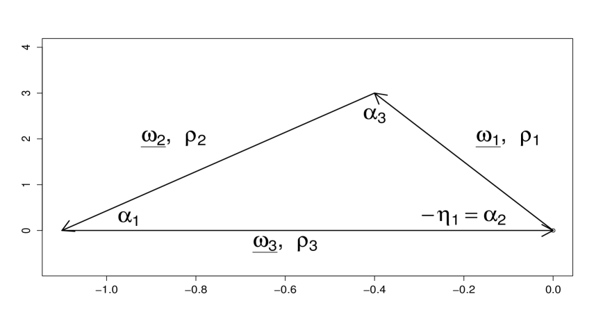
Figure 2. Triangle
Lemma 1 .
Let ρ k > 0 subscript 𝜌 𝑘 0 \rho_{k}>0 | ρ 2 − ρ 3 | ≤ ρ 1 ≤ ρ 2 + ρ 3 subscript 𝜌 2 subscript 𝜌 3 subscript 𝜌 1 subscript 𝜌 2 subscript 𝜌 3 \left|\rho_{2}-\rho_{3}\right|\leq\rho_{1}\leq\rho_{2}+\rho_{3} ρ 1 2 = ρ 2 2 + ρ 3 2 − 2 ρ 2 ρ 3 cos α 1 superscript subscript 𝜌 1 2 superscript subscript 𝜌 2 2 superscript subscript 𝜌 3 2 2 subscript 𝜌 2 subscript 𝜌 3 subscript 𝛼 1 \rho_{1}^{2}=\rho_{2}^{2}+\rho_{3}^{2}-2\rho_{2}\rho_{3}\cos\alpha_{1}
∫ 0 ∞ J ℓ 1 ( ρ 1 λ ) J ℓ 2 ( ρ 2 λ ) J ℓ 1 + ℓ 2 ( ρ 3 λ ) λ 𝑑 λ = cos ( ℓ 1 α 2 − ℓ 2 α 1 ) π ρ 2 ρ 3 sin α 1 , superscript subscript 0 subscript 𝐽 subscript ℓ 1 subscript 𝜌 1 𝜆 subscript 𝐽 subscript ℓ 2 subscript 𝜌 2 𝜆 subscript 𝐽 subscript ℓ 1 subscript ℓ 2 subscript 𝜌 3 𝜆 𝜆 differential-d 𝜆 subscript ℓ 1 subscript 𝛼 2 subscript ℓ 2 subscript 𝛼 1 𝜋 subscript 𝜌 2 subscript 𝜌 3 subscript 𝛼 1 \int_{0}^{\infty}J_{\ell_{1}}\left(\rho_{1}\lambda\right)J_{\ell_{2}}\left(\rho_{2}\lambda\right)J_{\ell_{1}+\ell_{2}}\left(\rho_{3}\lambda\right)\lambda d\lambda=\frac{\cos\left(\ell_{1}\alpha_{2}-\ell_{2}\alpha_{1}\right)}{\pi\rho_{2}\rho_{3}\sin\alpha_{1}},
otherwise if ρ 1 subscript 𝜌 1 \rho_{1} ρ 2 subscript 𝜌 2 \rho_{2}\ ρ 3 subscript 𝜌 3 \rho_{3}
Proof.
Formulae for integrals of Bessel functions require care and attention, see for
instance [Vil68 ] p224 and the Addition Theorem [Kor02 ] ,
p27. The assumptions imply that a triangle according to ( ρ 1 , ρ 2 , ρ 3 ) subscript 𝜌 1 subscript 𝜌 2 subscript 𝜌 3 \left(\rho_{1},\rho_{2},\rho_{3}\right) 2 ρ 1 2 = ρ 2 2 + ρ 3 2 − 2 ρ 2 ρ 3 cos α 1 superscript subscript 𝜌 1 2 superscript subscript 𝜌 2 2 superscript subscript 𝜌 3 2 2 subscript 𝜌 2 subscript 𝜌 3 subscript 𝛼 1 \rho_{1}^{2}=\rho_{2}^{2}+\rho_{3}^{2}-2\rho_{2}\rho_{3}\cos\alpha_{1} ρ 2 − ρ 3 cos α 1 = ρ 1 cos α 3 subscript 𝜌 2 subscript 𝜌 3 subscript 𝛼 1 subscript 𝜌 1 subscript 𝛼 3 \rho_{2}-\rho_{3}\cos\alpha_{1}=\rho_{1}\cos\alpha_{3} ρ 3 sin α 1 = ρ 1 sin α 3 subscript 𝜌 3 subscript 𝛼 1 subscript 𝜌 1 subscript 𝛼 3 \rho_{3}\sin\alpha_{1}=\rho_{1}\sin\alpha_{3} [EMOT81 ] , T2, p54 , equivalently, 4 ρ 2 2 ρ 3 2 − ( ρ 2 − ρ 2 2 − ρ 3 2 ) 2 = 2 ρ 2 ρ 3 sin α 1 4 superscript subscript 𝜌 2 2 superscript subscript 𝜌 3 2 superscript superscript 𝜌 2 superscript subscript 𝜌 2 2 superscript subscript 𝜌 3 2 2 2 subscript 𝜌 2 subscript 𝜌 3 subscript 𝛼 1 \sqrt{4\rho_{2}^{2}\rho_{3}^{2}-\left(\rho^{2}-\rho_{2}^{2}-\rho_{3}^{2}\right)^{2}}=2\rho_{2}\rho_{3}\sin\alpha_{1} α 1 ∈ ( 0 , π ) subscript 𝛼 1 0 𝜋 \alpha_{1}\in\left(0,\pi\right)
e i ℓ 1 α 2 J ℓ 1 ( ρ 1 ) = ∑ m = − ∞ ∞ J m ( ρ 2 ) J m + ℓ 1 ( ρ 3 ) e i m α 1 . superscript 𝑒 𝑖 subscript ℓ 1 subscript 𝛼 2 subscript 𝐽 subscript ℓ 1 subscript 𝜌 1 superscript subscript 𝑚 subscript 𝐽 𝑚 subscript 𝜌 2 subscript 𝐽 𝑚 subscript ℓ 1 subscript 𝜌 3 superscript 𝑒 𝑖 𝑚 subscript 𝛼 1 e^{i\ell_{1}\alpha_{2}}J_{\ell_{1}}\left(\rho_{1}\right)=\sum_{m=-\infty}^{\infty}J_{m}\left(\rho_{2}\right)J_{m+\ell_{1}}\left(\rho_{3}\right)e^{im\alpha_{1}}.
The system e i m α superscript 𝑒 𝑖 𝑚 𝛼 e^{im\alpha} [ 0 , 2 π ] 0 2 𝜋 \left[0,2\pi\right] α 1 subscript 𝛼 1 \alpha_{1} [ 0 , π ] 0 𝜋 \left[0,\pi\right]
∫ 0 π e i ( m − ℓ 2 ) α 𝑑 α = { π if m = ℓ 2 , i m − ℓ 2 ( 1 − ( − 1 ) m − ℓ 2 ) if m ≠ ℓ 2 , superscript subscript 0 𝜋 superscript 𝑒 𝑖 𝑚 subscript ℓ 2 𝛼 differential-d 𝛼 cases 𝜋 if 𝑚 subscript ℓ 2 𝑖 𝑚 subscript ℓ 2 1 superscript 1 𝑚 subscript ℓ 2 if 𝑚 subscript ℓ 2 \int_{0}^{\pi}e^{i\left(m-\ell_{2}\right)\alpha}d\alpha=\left\{\begin{array}[c]{ccc}\pi&\text{if }&m=\ell_{2},\\
\frac{i}{m-\ell_{2}}\left(1-\left(-1\right)^{m-\ell_{2}}\right)&\text{if }&m\neq\ell_{2},\end{array}\right.
hence
∫ 0 π e i ℓ 1 α 2 J ℓ 1 ( ρ 1 ) e − i ℓ 2 α 1 𝑑 α 1 = ∫ 0 π ∑ m = − ∞ ∞ J m ( ρ 2 ) J m + ℓ 1 ( ρ 3 ) e i ( m − ℓ 2 ) α 1 d α 1 = π J ℓ 2 ( ρ 2 ) J ℓ 1 + ℓ 2 ( ρ 3 ) + 2 i ∑ k = − ∞ ∞ 1 2 k + 1 J 2 k + 1 + ℓ 2 ( ρ 2 ) J 2 k + 1 + ℓ 1 + ℓ 2 ( ρ 3 ) . superscript subscript 0 𝜋 superscript 𝑒 𝑖 subscript ℓ 1 subscript 𝛼 2 subscript 𝐽 subscript ℓ 1 subscript 𝜌 1 superscript 𝑒 𝑖 subscript ℓ 2 subscript 𝛼 1 differential-d subscript 𝛼 1 superscript subscript 0 𝜋 superscript subscript 𝑚 subscript 𝐽 𝑚 subscript 𝜌 2 subscript 𝐽 𝑚 subscript ℓ 1 subscript 𝜌 3 superscript 𝑒 𝑖 𝑚 subscript ℓ 2 subscript 𝛼 1 𝑑 subscript 𝛼 1 𝜋 subscript 𝐽 subscript ℓ 2 subscript 𝜌 2 subscript 𝐽 subscript ℓ 1 subscript ℓ 2 subscript 𝜌 3 2 𝑖 superscript subscript 𝑘 1 2 𝑘 1 subscript 𝐽 2 𝑘 1 subscript ℓ 2 subscript 𝜌 2 subscript 𝐽 2 𝑘 1 subscript ℓ 1 subscript ℓ 2 subscript 𝜌 3 \int_{0}^{\pi}e^{i\ell_{1}\alpha_{2}}J_{\ell_{1}}\left(\rho_{1}\right)e^{-i\ell_{2}\alpha_{1}}d\alpha_{1}=\int_{0}^{\pi}\sum_{m=-\infty}^{\infty}J_{m}\left(\rho_{2}\right)J_{m+\ell_{1}}\left(\rho_{3}\right)e^{i\left(m-\ell_{2}\right)\alpha_{1}}d\alpha_{1}\\
=\pi J_{\ell_{2}}\left(\rho_{2}\right)J_{\ell_{1}+\ell_{2}}\left(\rho_{3}\right)+2i\sum_{k=-\infty}^{\infty}\frac{1}{2k+1}J_{2k+1+\ell_{2}}\left(\rho_{2}\right)J_{2k+1+\ell_{1}+\ell_{2}}\left(\rho_{3}\right).
The real part of the above equality provides
(A.1) ∫ 0 π cos ( ℓ 1 α 2 − ℓ 2 α 1 ) J ℓ 1 ( λ ρ 1 ) 𝑑 α 1 = π J ℓ 2 ( λ ρ 2 ) J ℓ 1 + ℓ 2 ( λ ρ 3 ) . superscript subscript 0 𝜋 subscript ℓ 1 subscript 𝛼 2 subscript ℓ 2 subscript 𝛼 1 subscript 𝐽 subscript ℓ 1 𝜆 subscript 𝜌 1 differential-d subscript 𝛼 1 𝜋 subscript 𝐽 subscript ℓ 2 𝜆 subscript 𝜌 2 subscript 𝐽 subscript ℓ 1 subscript ℓ 2 𝜆 subscript 𝜌 3 \int_{0}^{\pi}\cos\left(\ell_{1}\alpha_{2}-\ell_{2}\alpha_{1}\right)J_{\ell_{1}}\left(\lambda\rho_{1}\right)d\alpha_{1}=\pi J_{\ell_{2}}\left(\lambda\rho_{2}\right)J_{\ell_{1}+\ell_{2}}\left(\lambda\rho_{3}\right).
Now, integrate over λ d λ 𝜆 𝑑 𝜆 \lambda d\lambda B.1
∫ 0 ∞ J ℓ 1 ( ρ 1 λ ) J ℓ 2 ( ρ 2 λ ) J ℓ 1 + ℓ 2 ( ρ 3 λ ) λ 𝑑 λ superscript subscript 0 subscript 𝐽 subscript ℓ 1 subscript 𝜌 1 𝜆 subscript 𝐽 subscript ℓ 2 subscript 𝜌 2 𝜆 subscript 𝐽 subscript ℓ 1 subscript ℓ 2 subscript 𝜌 3 𝜆 𝜆 differential-d 𝜆 \displaystyle\int_{0}^{\infty}J_{\ell_{1}}\left(\rho_{1}\lambda\right)J_{\ell_{2}}\left(\rho_{2}\lambda\right)J_{\ell_{1}+\ell_{2}}\left(\rho_{3}\lambda\right)\lambda d\lambda
= ∫ 0 ∞ J ℓ 1 ( ρ 1 λ ) 1 π ∫ 0 π cos ( ℓ 1 α 2 − ℓ 2 γ ) J ℓ 1 ( ρ λ ) 𝑑 γ λ 𝑑 λ absent superscript subscript 0 subscript 𝐽 subscript ℓ 1 subscript 𝜌 1 𝜆 1 𝜋 superscript subscript 0 𝜋 subscript ℓ 1 subscript 𝛼 2 subscript ℓ 2 𝛾 subscript 𝐽 subscript ℓ 1 𝜌 𝜆 differential-d 𝛾 𝜆 differential-d 𝜆 \displaystyle=\int_{0}^{\infty}J_{\ell_{1}}\left(\rho_{1}\lambda\right)\frac{1}{\pi}\int_{0}^{\pi}\cos\left(\ell_{1}\alpha_{2}-\ell_{2}\gamma\right)J_{\ell_{1}}\left(\rho\lambda\right)d\gamma\lambda d\lambda
= 1 π ∫ | ρ 2 − ρ 3 | ρ 2 + ρ 3 ∫ 0 ∞ J ℓ 1 ( ρ 1 λ ) J ℓ 1 ( ρ λ ) λ 𝑑 λ cos ( ℓ 1 α 2 − ℓ 2 γ ) ρ d ρ ρ 2 ρ 3 sin γ absent 1 𝜋 superscript subscript subscript 𝜌 2 subscript 𝜌 3 subscript 𝜌 2 subscript 𝜌 3 superscript subscript 0 subscript 𝐽 subscript ℓ 1 subscript 𝜌 1 𝜆 subscript 𝐽 subscript ℓ 1 𝜌 𝜆 𝜆 differential-d 𝜆 subscript ℓ 1 subscript 𝛼 2 subscript ℓ 2 𝛾 𝜌 𝑑 𝜌 subscript 𝜌 2 subscript 𝜌 3 𝛾 \displaystyle=\frac{1}{\pi}\int_{\left|\rho_{2}-\rho_{3}\right|}^{\rho_{2}+\rho_{3}}\int_{0}^{\infty}J_{\ell_{1}}\left(\rho_{1}\lambda\right)J_{\ell_{1}}\left(\rho\lambda\right)\lambda d\lambda\frac{\cos\left(\ell_{1}\alpha_{2}-\ell_{2}\gamma\right)\rho d\rho}{\rho_{2}\rho_{3}\sin\gamma}
= 1 π ∫ | ρ 2 − ρ 3 | ρ 2 + ρ 3 cos ( ℓ 1 α 2 − ℓ 2 γ ) ρ 2 ρ 3 sin γ δ ( ρ 1 − ρ ) ρ 1 ρ 𝑑 ρ absent 1 𝜋 superscript subscript subscript 𝜌 2 subscript 𝜌 3 subscript 𝜌 2 subscript 𝜌 3 subscript ℓ 1 subscript 𝛼 2 subscript ℓ 2 𝛾 subscript 𝜌 2 subscript 𝜌 3 𝛾 𝛿 subscript 𝜌 1 𝜌 subscript 𝜌 1 𝜌 differential-d 𝜌 \displaystyle=\frac{1}{\pi}\int_{\left|\rho_{2}-\rho_{3}\right|}^{\rho_{2}+\rho_{3}}\frac{\cos\left(\ell_{1}\alpha_{2}-\ell_{2}\gamma\right)}{\rho_{2}\rho_{3}\sin\gamma}\frac{\delta\left(\rho_{1}-\rho\right)}{\rho_{1}}\rho d\rho
= cos ( ℓ 1 α 2 − ℓ 2 α 1 ) π ρ 2 ρ 3 sin α 1 . absent subscript ℓ 1 subscript 𝛼 2 subscript ℓ 2 subscript 𝛼 1 𝜋 subscript 𝜌 2 subscript 𝜌 3 subscript 𝛼 1 \displaystyle=\frac{\cos\left(\ell_{1}\alpha_{2}-\ell_{2}\alpha_{1}\right)}{\pi\rho_{2}\rho_{3}\sin\alpha_{1}}.
The integral is zero if the inequality | ρ 2 − ρ 3 | ≤ ρ 1 ≤ ρ 2 + ρ 3 subscript 𝜌 2 subscript 𝜌 3 subscript 𝜌 1 subscript 𝜌 2 subscript 𝜌 3 \left|\rho_{2}-\rho_{3}\right|\leq\rho_{1}\leq\rho_{2}+\rho_{3} [Vil68 ] p. 224.
∎
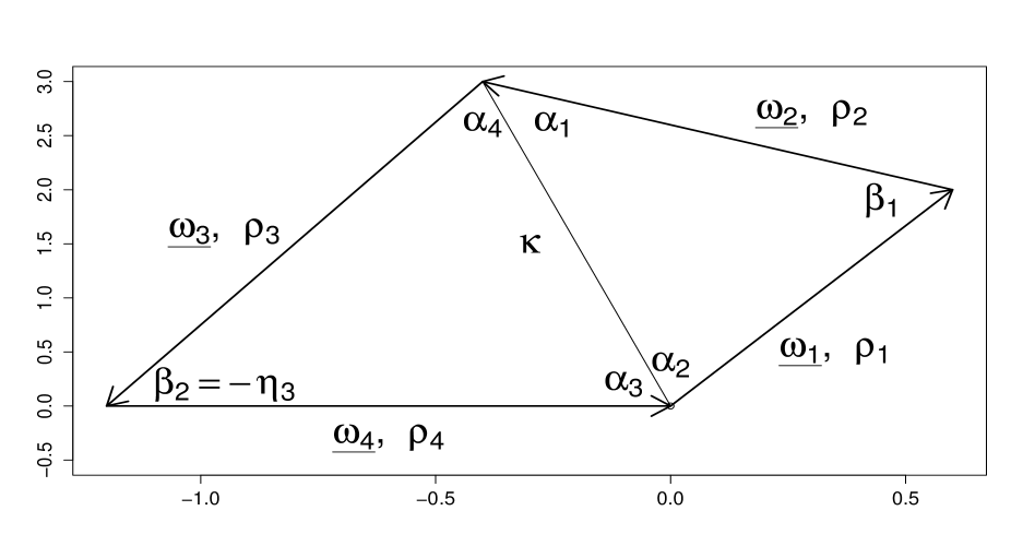
We consider a quadrilateral according to the wave numbers ( α 1 , ρ 2 , ρ 3 , ρ 4 ) subscript 𝛼 1 subscript 𝜌 2 subscript 𝜌 3 subscript 𝜌 4 \left(\alpha_{1},\rho_{2},\rho_{3},\rho_{4}\right) ( ρ 1 , ρ 2 , κ ) subscript 𝜌 1 subscript 𝜌 2 𝜅 \left(\rho_{1},\rho_{2},\kappa\right) ( κ , ρ 3 , ρ 4 ) 𝜅 subscript 𝜌 3 subscript 𝜌 4 \left(\kappa,\rho_{3},\rho_{4}\right) κ = | κ ¯ | 𝜅 ¯ 𝜅 \kappa=\left|\underline{\kappa}\right| ρ j = | ω ¯ j | subscript 𝜌 𝑗 subscript ¯ 𝜔 𝑗 \rho_{j}=\left|\underline{\omega}_{j}\right| 3 ( ω ¯ 1 , ω ¯ 2 , κ ¯ ) subscript ¯ 𝜔 1 subscript ¯ 𝜔 2 ¯ 𝜅 \left(\underline{\omega}_{1},\underline{\omega}_{2},\underline{\kappa}\right) ( ω ¯ 3 , ω ¯ 4 , − κ ¯ ) subscript ¯ 𝜔 3 subscript ¯ 𝜔 4 ¯ 𝜅 \left(\underline{\omega}_{3},\underline{\omega}_{4},-\underline{\kappa}\right) ( ρ 1 , ρ 2 , κ ) subscript 𝜌 1 subscript 𝜌 2 𝜅 \left(\rho_{1},\rho_{2},\kappa\right) ( κ , ρ 3 , ρ 4 ) 𝜅 subscript 𝜌 3 subscript 𝜌 4 \left(\kappa,\rho_{3},\rho_{4}\right)
max ( | ρ 2 − ρ 1 | , | ρ 4 − ρ 3 | ) < κ < min ( ρ 1 + ρ 2 , ρ 3 + ρ 4 ) , subscript 𝜌 2 subscript 𝜌 1 subscript 𝜌 4 subscript 𝜌 3 𝜅 subscript 𝜌 1 subscript 𝜌 2 subscript 𝜌 3 subscript 𝜌 4 \max\left(\left|\rho_{2}-\rho_{1}\right|,\left|\rho_{4}-\rho_{3}\right|\right)<\kappa<\min\left(\rho_{1}+\rho_{2},\rho_{3}+\rho_{4}\right),
fulfils, see Figure 3
Figure 3. Quadrilateral
Lemma 2 .
Assume κ 2 = ρ 3 2 + ρ 4 2 − 2 ρ 3 ρ 4 cos β 2 superscript 𝜅 2 superscript subscript 𝜌 3 2 superscript subscript 𝜌 4 2 2 subscript 𝜌 3 subscript 𝜌 4 subscript 𝛽 2 \kappa^{2}=\rho_{3}^{2}+\rho_{4}^{2}-2\rho_{3}\rho_{4}\cos\beta_{2} β 2 ∈ ( 0 , π ) subscript 𝛽 2 0 𝜋 \beta_{2}\in\left(0,\pi\right) ( ρ 1 , ρ 2 , κ ) subscript 𝜌 1 subscript 𝜌 2 𝜅 \left(\rho_{1},\rho_{2},\kappa\right) 3
∫ 0 ∞ J ℓ 1 ( ρ 1 λ ) J ℓ 2 ( ρ 2 λ ) J ℓ 3 ( ρ 3 λ ) J ℓ 1 + ℓ 2 + ℓ 3 ( ρ 4 λ ) λ 𝑑 λ = 1 π 2 ∫ 0 π cos ( ( ℓ 1 + ℓ 2 ) α 3 − ℓ 3 β 2 ) cos ( ℓ 1 α 2 − ℓ 2 α 1 ) ρ 2 κ sin α 1 χ ( △ | ρ 1 , ρ 2 , κ ) d β 2 , \int_{0}^{\infty}J_{\ell_{1}}\left(\rho_{1}\lambda\right)J_{\ell_{2}}\left(\rho_{2}\lambda\right)J_{\ell_{3}}\left(\rho_{3}\lambda\right)J_{\ell_{1}+\ell_{2}+\ell_{3}}\left(\rho_{4}\lambda\right)\lambda d\lambda\\
=\frac{1}{\pi^{2}}\int_{0}^{\pi}\cos\left(\left(\ell_{1}+\ell_{2}\right)\alpha_{3}-\ell_{3}\beta_{2}\right)\frac{\cos\left(\ell_{1}\alpha_{2}-\ell_{2}\alpha_{1}\right)}{\rho_{2}\kappa\sin\alpha_{1}}\chi\left(\bigtriangleup|\rho_{1},\rho_{2},\kappa\right)d\beta_{2},
where the notations correspond to the Figure 3 χ ( △ | ρ 1 , ρ 2 , κ ) \chi\left(\bigtriangleup|\rho_{1},\rho_{2},\kappa\right) ( ρ 1 , ρ 2 , κ ) subscript 𝜌 1 subscript 𝜌 2 𝜅 \left(\rho_{1},\rho_{2},\kappa\right) 1 1 1
Proof.
The equation (A.1 1
J ℓ 3 ( ρ 3 λ ) J ℓ 1 + ℓ 2 + ℓ 3 ( ρ 4 λ ) subscript 𝐽 subscript ℓ 3 subscript 𝜌 3 𝜆 subscript 𝐽 subscript ℓ 1 subscript ℓ 2 subscript ℓ 3 subscript 𝜌 4 𝜆 \displaystyle J_{\ell_{3}}\left(\rho_{3}\lambda\right)J_{\ell_{1}+\ell_{2}+\ell_{3}}\left(\rho_{4}\lambda\right) = 1 π ∫ | ρ 4 − ρ 3 | ρ 3 + ρ 4 J ℓ 1 + ℓ 2 ( κ λ ) cos ( ( ℓ 1 + ℓ 2 ) α 3 − ℓ 3 β 2 ) κ d κ ρ 3 ρ 4 sin β 2 , absent 1 𝜋 superscript subscript subscript 𝜌 4 subscript 𝜌 3 subscript 𝜌 3 subscript 𝜌 4 subscript 𝐽 subscript ℓ 1 subscript ℓ 2 𝜅 𝜆 subscript ℓ 1 subscript ℓ 2 subscript 𝛼 3 subscript ℓ 3 subscript 𝛽 2 𝜅 𝑑 𝜅 subscript 𝜌 3 subscript 𝜌 4 subscript 𝛽 2 \displaystyle=\frac{1}{\pi}\int_{\left|\rho_{4}-\rho_{3}\right|}^{\rho_{3}+\rho_{4}}J_{\ell_{1}+\ell_{2}}\left(\kappa\lambda\right)\frac{\cos\left(\left(\ell_{1}+\ell_{2}\right)\alpha_{3}-\ell_{3}\beta_{2}\right)\kappa d\kappa}{\rho_{3}\rho_{4}\sin\beta_{2}},
∫ 0 ∞ J ℓ 1 ( ρ 1 λ ) J ℓ 2 ( ρ 2 λ ) J ℓ 1 + ℓ 2 ( κ λ ) λ 𝑑 λ superscript subscript 0 subscript 𝐽 subscript ℓ 1 subscript 𝜌 1 𝜆 subscript 𝐽 subscript ℓ 2 subscript 𝜌 2 𝜆 subscript 𝐽 subscript ℓ 1 subscript ℓ 2 𝜅 𝜆 𝜆 differential-d 𝜆 \displaystyle\int_{0}^{\infty}J_{\ell_{1}}\left(\rho_{1}\lambda\right)J_{\ell_{2}}\left(\rho_{2}\lambda\right)J_{\ell_{1}+\ell_{2}}\left(\kappa\lambda\right)\lambda d\lambda = cos ( ℓ 1 α 2 − ℓ 2 α 1 ) π ρ 1 κ sin α 2 χ ( △ | ρ 1 , ρ 2 , κ ) , \displaystyle=\frac{\cos\left(\ell_{1}\alpha_{2}-\ell_{2}\alpha_{1}\right)}{\pi\rho_{1}\kappa\sin\alpha_{2}}\chi\left(\bigtriangleup|\rho_{1},\rho_{2},\kappa\right),
hence
∫ 0 ∞ J ℓ 1 ( ρ 1 λ ) J ℓ 2 ( ρ 2 λ ) J ℓ 3 ( ρ 3 λ ) J ℓ 1 + ℓ 2 + ℓ 3 ( ρ 4 λ ) λ 𝑑 λ superscript subscript 0 subscript 𝐽 subscript ℓ 1 subscript 𝜌 1 𝜆 subscript 𝐽 subscript ℓ 2 subscript 𝜌 2 𝜆 subscript 𝐽 subscript ℓ 3 subscript 𝜌 3 𝜆 subscript 𝐽 subscript ℓ 1 subscript ℓ 2 subscript ℓ 3 subscript 𝜌 4 𝜆 𝜆 differential-d 𝜆 \displaystyle\int_{0}^{\infty}J_{\ell_{1}}\left(\rho_{1}\lambda\right)J_{\ell_{2}}\left(\rho_{2}\lambda\right)J_{\ell_{3}}\left(\rho_{3}\lambda\right)J_{\ell_{1}+\ell_{2}+\ell_{3}}\left(\rho_{4}\lambda\right)\lambda d\lambda
= 1 π ∫ | ρ 4 − ρ 3 | ρ 4 + ρ 3 cos ( ( ℓ 1 + ℓ 2 ) α 3 − ℓ 3 β 2 ) ρ 3 ρ 4 sin β 2 ∫ 0 ∞ J ℓ 1 ( ρ 1 λ ) J ℓ 2 ( ρ 2 λ ) J ℓ 1 + ℓ 2 ( κ λ ) λ 𝑑 λ κ 𝑑 κ absent 1 𝜋 superscript subscript subscript 𝜌 4 subscript 𝜌 3 subscript 𝜌 4 subscript 𝜌 3 subscript ℓ 1 subscript ℓ 2 subscript 𝛼 3 subscript ℓ 3 subscript 𝛽 2 subscript 𝜌 3 subscript 𝜌 4 subscript 𝛽 2 superscript subscript 0 subscript 𝐽 subscript ℓ 1 subscript 𝜌 1 𝜆 subscript 𝐽 subscript ℓ 2 subscript 𝜌 2 𝜆 subscript 𝐽 subscript ℓ 1 subscript ℓ 2 𝜅 𝜆 𝜆 differential-d 𝜆 𝜅 differential-d 𝜅 \displaystyle=\frac{1}{\pi}\int_{\left|\rho_{4}-\rho_{3}\right|}^{\rho_{4}+\rho_{3}}\frac{\cos\left(\left(\ell_{1}+\ell_{2}\right)\alpha_{3}-\ell_{3}\beta_{2}\right)}{\rho_{3}\rho_{4}\sin\beta_{2}}\int_{0}^{\infty}J_{\ell_{1}}\left(\rho_{1}\lambda\right)J_{\ell_{2}}\left(\rho_{2}\lambda\right)J_{\ell_{1}+\ell_{2}}\left(\kappa\lambda\right)\lambda d\lambda\kappa d\kappa
= 1 π 2 ∫ | ρ 4 − ρ 3 | ρ 4 + ρ 3 cos ( ( ℓ 1 + ℓ 2 ) α 3 − ℓ 3 β 2 ) ρ 3 ρ 4 sin β 2 cos ( ℓ 1 α 2 − ℓ 2 α 1 ) ρ 1 κ sin α 2 χ ( △ | ρ 1 , ρ 2 , κ ) κ d κ \displaystyle=\frac{1}{\pi^{2}}\int_{\left|\rho_{4}-\rho_{3}\right|}^{\rho_{4}+\rho_{3}}\frac{\cos\left(\left(\ell_{1}+\ell_{2}\right)\alpha_{3}-\ell_{3}\beta_{2}\right)}{\rho_{3}\rho_{4}\sin\beta_{2}}\frac{\cos\left(\ell_{1}\alpha_{2}-\ell_{2}\alpha_{1}\right)}{\rho_{1}\kappa\sin\alpha_{2}}\chi\left(\bigtriangleup|\rho_{1},\rho_{2},\kappa\right)\kappa d\kappa
= 1 π 2 ∫ 0 π cos ( ( ℓ 1 + ℓ 2 ) α 3 − ℓ 3 β 2 ) cos ( ℓ 1 α 2 − ℓ 2 α 1 ) ρ 2 κ sin α 1 χ ( △ | ρ 1 , ρ 2 , κ ) d β 2 , \displaystyle=\frac{1}{\pi^{2}}\int_{0}^{\pi}\cos\left(\left(\ell_{1}+\ell_{2}\right)\alpha_{3}-\ell_{3}\beta_{2}\right)\frac{\cos\left(\ell_{1}\alpha_{2}-\ell_{2}\alpha_{1}\right)}{\rho_{2}\kappa\sin\alpha_{1}}\chi\left(\bigtriangleup|\rho_{1},\rho_{2},\kappa\right)d\beta_{2},
where ( 2 ρ 3 ρ 4 ) 2 − ( κ 2 − ρ 3 2 − ρ 4 2 ) 2 = 2 ρ 3 ρ 4 sin β 2 superscript 2 subscript 𝜌 3 subscript 𝜌 4 2 superscript superscript 𝜅 2 superscript subscript 𝜌 3 2 superscript subscript 𝜌 4 2 2 2 subscript 𝜌 3 subscript 𝜌 4 subscript 𝛽 2 \sqrt{\left(2\rho_{3}\rho_{4}\right)^{2}-\left(\kappa^{2}-\rho_{3}^{2}-\rho_{4}^{2}\right)^{2}}=2\rho_{3}\rho_{4}\sin\beta_{2} κ d κ = ρ 3 ρ 4 sin ( β 2 ) d β 2 𝜅 𝑑 𝜅 subscript 𝜌 3 subscript 𝜌 4 subscript 𝛽 2 𝑑 subscript 𝛽 2 \kappa d\kappa=\rho_{3}\rho_{4}\sin\left(\beta_{2}\right)d\beta_{2} ρ 1 sin β 1 = κ sin α 1 subscript 𝜌 1 subscript 𝛽 1 𝜅 subscript 𝛼 1 \rho_{1}\sin\beta_{1}=\kappa\sin\alpha_{1} 3 ( ρ 1 , ρ 2 , ρ 3 , ρ 4 ) subscript 𝜌 1 subscript 𝜌 2 subscript 𝜌 3 subscript 𝜌 4 \left(\rho_{1},\rho_{2},\rho_{3},\rho_{4}\right) κ 𝜅 \kappa β 2 subscript 𝛽 2 \beta_{2}
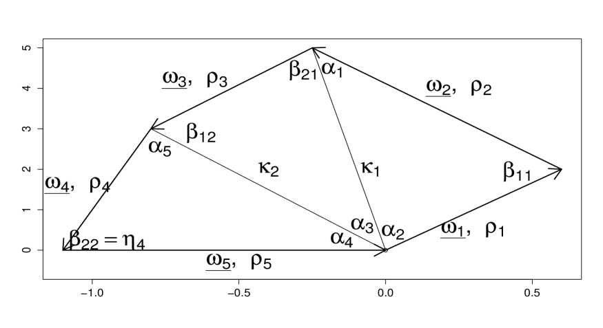
For further generalization of Lemma 1 5 5 5 5 5 5 2 2 2 4 κ 2 = | κ ¯ 2 | subscript 𝜅 2 subscript ¯ 𝜅 2 \kappa_{2}=\left|\underline{\kappa}_{2}\right| β 2 , 2 subscript 𝛽 2 2
\beta_{2,2} ρ 4 = | ω ¯ 4 | subscript 𝜌 4 subscript ¯ 𝜔 4 \rho_{4}=\left|\underline{\omega}_{4}\right| ρ 5 = | ω ¯ 5 | subscript 𝜌 5 subscript ¯ 𝜔 5 \rho_{5}=\left|\underline{\omega}_{5}\right|
Figure 4. Multilateral
Theorem 3 .
Let p ≥ 4 𝑝 4 p\geq 4 p 𝑝 p
∫ 0 ∞ J Σ 1 p − 1 ℓ k ( ρ p λ ) ∏ k = 1 p − 1 J ℓ k ( ρ k λ ) λ d λ = 1 π p − 2 ∫ 0 π ⋯ ∫ 0 π cos ( ℓ 1 α 2 − ℓ 2 α 1 ) ρ 2 κ 1 sin ( α 1 ) ∏ k = 2 p − 2 cos ( α k + 1 ∑ j = 1 k ℓ j − ℓ k + 1 β k − 1 , 2 ) χ ( △ | ρ k + 2 , κ k , κ k + 1 ) d β k − 1 , 2 , \int_{0}^{\infty}J_{\Sigma_{1}^{p-1}\ell_{k}}\left(\rho_{p}\lambda\right)\prod\limits_{k=1}^{p-1}J_{\ell_{k}}\left(\rho_{k}\lambda\right)\lambda d\lambda\\
=\frac{1}{\pi^{p-2}}\int_{0}^{\pi}\cdots\int_{0}^{\pi}\frac{\cos\left(\ell_{1}\alpha_{2}-\ell_{2}\alpha_{1}\right)}{\rho_{2}\kappa_{1}\sin\left(\alpha_{1}\right)}\prod\limits_{k=2}^{p-2}\cos\left(\alpha_{k+1}{\textstyle\sum_{j=1}^{k}}\ell_{j}-\ell_{k+1}\beta_{k-1,2}\right)\chi\left(\bigtriangleup|\rho_{k+2},\kappa_{k},\kappa_{k+1}\right)d\beta_{k-1,2},
where each angle α k subscript 𝛼 𝑘 \alpha_{k} ρ k subscript 𝜌 𝑘 \rho_{k} β k , 1 subscript 𝛽 𝑘 1
\beta_{k,1} β k , 2 subscript 𝛽 𝑘 2
\beta_{k,2} κ k subscript 𝜅 𝑘 \kappa_{k} 4
Proof.
A multilateral can be split up p − 2 𝑝 2 p-2 4 p = 4 𝑝 4 p=4 p = 5 𝑝 5 p=5
J ℓ 4 ( ρ 4 λ ) J ℓ 1 + ℓ 2 + ℓ 3 + ℓ 4 ( ρ 5 λ ) = 1 π ∫ 0 π J ℓ 1 + ℓ 2 + ℓ 3 ( κ 2 λ ) cos ( ( ℓ 1 + ℓ 2 + ℓ 3 ) α 4 − ℓ 4 β 2 , 2 ) 𝑑 β 2 , 2 , subscript 𝐽 subscript ℓ 4 subscript 𝜌 4 𝜆 subscript 𝐽 subscript ℓ 1 subscript ℓ 2 subscript ℓ 3 subscript ℓ 4 subscript 𝜌 5 𝜆 1 𝜋 superscript subscript 0 𝜋 subscript 𝐽 subscript ℓ 1 subscript ℓ 2 subscript ℓ 3 subscript 𝜅 2 𝜆 subscript ℓ 1 subscript ℓ 2 subscript ℓ 3 subscript 𝛼 4 subscript ℓ 4 subscript 𝛽 2 2
differential-d subscript 𝛽 2 2
J_{\ell_{4}}\left(\rho_{4}\lambda\right)J_{\ell_{1}+\ell_{2}+\ell_{3}+\ell_{4}}\left(\rho_{5}\lambda\right)=\frac{1}{\pi}\int_{0}^{\pi}J_{\ell_{1}+\ell_{2}+\ell_{3}}\left(\kappa_{2}\lambda\right)\cos\left(\left(\ell_{1}+\ell_{2}+\ell_{3}\right)\alpha_{4}-\ell_{4}\beta_{2,2}\right)d\beta_{2,2},
and the result of Lemma 2
∫ 0 ∞ J ℓ 1 ( ρ 1 λ ) J ℓ 2 ( ρ 2 λ ) J ℓ 3 ( ρ 3 λ ) J ℓ 1 + ℓ 2 + ℓ 3 ( κ 2 λ ) λ 𝑑 λ = 1 π 2 ∫ 0 π cos ( ( ℓ 1 + ℓ 2 ) α 3 − ℓ 3 β 1 , 2 ) cos ( ℓ 1 α 2 − ℓ 2 α 1 ) d β 1 , 2 ρ 2 κ 1 sin α 1 superscript subscript 0 subscript 𝐽 subscript ℓ 1 subscript 𝜌 1 𝜆 subscript 𝐽 subscript ℓ 2 subscript 𝜌 2 𝜆 subscript 𝐽 subscript ℓ 3 subscript 𝜌 3 𝜆 subscript 𝐽 subscript ℓ 1 subscript ℓ 2 subscript ℓ 3 subscript 𝜅 2 𝜆 𝜆 differential-d 𝜆 1 superscript 𝜋 2 superscript subscript 0 𝜋 subscript ℓ 1 subscript ℓ 2 subscript 𝛼 3 subscript ℓ 3 subscript 𝛽 1 2
subscript ℓ 1 subscript 𝛼 2 subscript ℓ 2 subscript 𝛼 1 𝑑 subscript 𝛽 1 2
subscript 𝜌 2 subscript 𝜅 1 subscript 𝛼 1 \int_{0}^{\infty}J_{\ell_{1}}\left(\rho_{1}\lambda\right)J_{\ell_{2}}\left(\rho_{2}\lambda\right)J_{\ell_{3}}\left(\rho_{3}\lambda\right)J_{\ell_{1}+\ell_{2}+\ell_{3}}\left(\kappa_{2}\lambda\right)\lambda d\lambda\\
=\frac{1}{\pi^{2}}\int_{0}^{\pi}\cos\left(\left(\ell_{1}+\ell_{2}\right)\alpha_{3}-\ell_{3}\beta_{1,2}\right)\cos\left(\ell_{1}\alpha_{2}-\ell_{2}\alpha_{1}\right)\frac{d\beta_{1,2}}{\rho_{2}\kappa_{1}\sin\alpha_{1}}
hence we obtain
∫ 0 ∞ J ℓ 1 ( ρ 1 λ ) J ℓ 2 ( ρ 2 λ ) J ℓ 3 ( ρ 3 λ ) J ℓ 4 ( ρ 4 λ ) J ℓ 1 + ℓ 2 + ℓ 3 + ℓ 4 ( ρ 5 λ ) λ 𝑑 λ superscript subscript 0 subscript 𝐽 subscript ℓ 1 subscript 𝜌 1 𝜆 subscript 𝐽 subscript ℓ 2 subscript 𝜌 2 𝜆 subscript 𝐽 subscript ℓ 3 subscript 𝜌 3 𝜆 subscript 𝐽 subscript ℓ 4 subscript 𝜌 4 𝜆 subscript 𝐽 subscript ℓ 1 subscript ℓ 2 subscript ℓ 3 subscript ℓ 4 subscript 𝜌 5 𝜆 𝜆 differential-d 𝜆 \displaystyle\int_{0}^{\infty}J_{\ell_{1}}\left(\rho_{1}\lambda\right)J_{\ell_{2}}\left(\rho_{2}\lambda\right)J_{\ell_{3}}\left(\rho_{3}\lambda\right)J_{\ell_{4}}\left(\rho_{4}\lambda\right)J_{\ell_{1}+\ell_{2}+\ell_{3}+\ell_{4}}\left(\rho_{5}\lambda\right)\lambda d\lambda
= 1 π 3 ∫ 0 ∞ J ℓ 1 ( ρ 1 λ ) J ℓ 2 ( ρ 2 λ ) J ℓ 3 ( ρ 3 λ ) ∫ 0 π J ℓ 1 + ℓ 2 + ℓ 3 ( κ 2 λ ) cos ( ( ℓ 1 + ℓ 2 + ℓ 3 ) α 4 − ℓ 4 β 2 , 2 ) 𝑑 β 2 , 2 λ 𝑑 λ absent 1 superscript 𝜋 3 superscript subscript 0 subscript 𝐽 subscript ℓ 1 subscript 𝜌 1 𝜆 subscript 𝐽 subscript ℓ 2 subscript 𝜌 2 𝜆 subscript 𝐽 subscript ℓ 3 subscript 𝜌 3 𝜆 superscript subscript 0 𝜋 subscript 𝐽 subscript ℓ 1 subscript ℓ 2 subscript ℓ 3 subscript 𝜅 2 𝜆 subscript ℓ 1 subscript ℓ 2 subscript ℓ 3 subscript 𝛼 4 subscript ℓ 4 subscript 𝛽 2 2
differential-d subscript 𝛽 2 2
𝜆 differential-d 𝜆 \displaystyle=\frac{1}{\pi^{3}}\int_{0}^{\infty}J_{\ell_{1}}\left(\rho_{1}\lambda\right)J_{\ell_{2}}\left(\rho_{2}\lambda\right)J_{\ell_{3}}\left(\rho_{3}\lambda\right)\int_{0}^{\pi}J_{\ell_{1}+\ell_{2}+\ell_{3}}\left(\kappa_{2}\lambda\right)\cos\left(\left(\ell_{1}+\ell_{2}+\ell_{3}\right)\alpha_{4}-\ell_{4}\beta_{2,2}\right)d\beta_{2,2}\lambda d\lambda
= 1 π 3 ∫ 0 π ∫ 0 π cos ( ℓ 1 α 2 − ℓ 2 α 1 ) cos ( ( ℓ 1 + ℓ 2 ) α 3 − ℓ 3 β 1 , 2 ) cos ( ( ℓ 1 + ℓ 2 + ℓ 3 ) α 4 − ℓ 4 β 2 , 2 ) d β 2 , 2 d β 1 , 2 ρ 2 κ 1 sin α 1 . absent 1 superscript 𝜋 3 superscript subscript 0 𝜋 superscript subscript 0 𝜋 subscript ℓ 1 subscript 𝛼 2 subscript ℓ 2 subscript 𝛼 1 subscript ℓ 1 subscript ℓ 2 subscript 𝛼 3 subscript ℓ 3 subscript 𝛽 1 2
subscript ℓ 1 subscript ℓ 2 subscript ℓ 3 subscript 𝛼 4 subscript ℓ 4 subscript 𝛽 2 2
𝑑 subscript 𝛽 2 2
𝑑 subscript 𝛽 1 2
subscript 𝜌 2 subscript 𝜅 1 subscript 𝛼 1 \displaystyle=\frac{1}{\pi^{3}}\int_{0}^{\pi}\int_{0}^{\pi}\cos\left(\ell_{1}\alpha_{2}-\ell_{2}\alpha_{1}\right)\cos\left(\left(\ell_{1}+\ell_{2}\right)\alpha_{3}-\ell_{3}\beta_{1,2}\right)\frac{\cos\left(\left(\ell_{1}+\ell_{2}+\ell_{3}\right)\alpha_{4}-\ell_{4}\beta_{2,2}\right)d\beta_{2,2}d\beta_{1,2}}{\rho_{2}\kappa_{1}\sin\alpha_{1}}.
Appendix C Cumulants of spectral measures Z ℓ ( ρ d ρ ) subscript 𝑍 ℓ 𝜌 𝑑 𝜌 Z_{\ell}\left(\rho d\rho\right)
We generalize the joint cumulant stochastic spectral measures
Cum ( Z 0 ( ρ 1 d ρ 1 ) , Z ℓ ( ρ 2 d ρ 2 ) , Z − ℓ ( ρ 3 d ρ 3 ) ) = 2 ( − 1 ) ℓ χ ( △ | ρ 1 , ρ 2 , ρ 3 ) cos ( ℓ arccos ( R ) ) ρ 2 ρ 3 1 − R 2 S 3 ( ρ 1 , ρ 2 , ρ 3 ) ∏ k = 1 3 ρ k d ρ k , \operatorname*{Cum}\left(Z_{0}\left(\rho_{1}d\rho_{1}\right),Z_{\ell}\left(\rho_{2}d\rho_{2}\right),Z_{-\ell}\left(\rho_{3}d\rho_{3}\right)\right)\\
=2\left(-1\right)^{\ell}\chi\left(\bigtriangleup|\rho_{1},\rho_{2},\rho_{3}\right)\frac{\cos\left(\ell\arccos\left(R\right)\right)}{\rho_{2}\rho_{3}\sqrt{1-R^{2}}}S_{3}\left(\rho_{1},\rho_{2},\rho_{3}\right){\textstyle\prod\limits_{k=1}^{3}}\rho_{k}d\rho_{k},
where R = ( ρ 2 2 + ρ 3 2 − ρ 1 2 ) / ( 2 ρ 2 ρ 3 ) = cos α 1 𝑅 superscript subscript 𝜌 2 2 superscript subscript 𝜌 3 2 superscript subscript 𝜌 1 2 2 subscript 𝜌 2 subscript 𝜌 3 subscript 𝛼 1 R=\left(\rho_{2}^{2}+\rho_{3}^{2}-\rho_{1}^{2}\right)/\left(2\rho_{2}\rho_{3}\right)=\cos\alpha_{1} χ ( △ | ρ 1 , ρ 2 , ρ 3 ) = 1 \chi\left(\bigtriangleup|\rho_{1},\rho_{2},\rho_{3}\right)=1 ρ 1 , ρ 2 , ρ 3 subscript 𝜌 1 subscript 𝜌 2 subscript 𝜌 3
\rho_{1},\rho_{2},\rho_{3}\ 0 0 [Ter14 ] in order
to get the formula for trispectrum and higher order spectra. χ ( △ | ρ 1 , ρ 2 , ρ 3 ) \chi\left(\bigtriangleup|\rho_{1},\rho_{2},\rho_{3}\right) ρ 1 subscript 𝜌 1 \rho_{1} ρ 2 subscript 𝜌 2 \rho_{2} ρ 3 subscript 𝜌 3 \rho_{3}
Consider the fourth order cumulant
Cum ( Z 0 ( ρ 1 d ρ 1 ) , Z ℓ 2 ( ρ 2 d ρ 2 ) , Z ℓ 3 ( ρ 3 d ρ 3 ) , Z − ( ℓ 2 + ℓ 3 ) ( ρ 4 d ρ 4 ) ) = ⨌ 0 2 π e − i ℓ 2 ( η 2 − η 4 ) − i ℓ 3 ( η 3 − η 4 ) δ ( Σ 1 4 ρ k ω ¯ ^ k ) S 4 ( α 1 , ρ 2 : 4 , β 2 ) ∏ k = 1 4 d η k ∏ k = 1 4 ρ k d ρ k , Cum subscript 𝑍 0 subscript 𝜌 1 𝑑 subscript 𝜌 1 subscript 𝑍 subscript ℓ 2 subscript 𝜌 2 𝑑 subscript 𝜌 2 subscript 𝑍 subscript ℓ 3 subscript 𝜌 3 𝑑 subscript 𝜌 3 subscript 𝑍 subscript ℓ 2 subscript ℓ 3 subscript 𝜌 4 𝑑 subscript 𝜌 4 superscript subscript quadruple-integral 0 2 𝜋 superscript 𝑒 𝑖 subscript ℓ 2 subscript 𝜂 2 subscript 𝜂 4 𝑖 subscript ℓ 3 subscript 𝜂 3 subscript 𝜂 4 𝛿 superscript subscript Σ 1 4 subscript 𝜌 𝑘 subscript ¯ ^ 𝜔 𝑘 subscript 𝑆 4 subscript 𝛼 1 subscript 𝜌 : 2 4 subscript 𝛽 2 superscript subscript product 𝑘 1 4 𝑑 subscript 𝜂 𝑘 superscript subscript product 𝑘 1 4 subscript 𝜌 𝑘 𝑑 subscript 𝜌 𝑘 \operatorname*{Cum}\left(Z_{0}\left(\rho_{1}d\rho_{1}\right),Z_{\ell_{2}}\left(\rho_{2}d\rho_{2}\right),Z_{\ell_{3}}\left(\rho_{3}d\rho_{3}\right),Z_{-\left(\ell_{2}+\ell_{3}\right)}\left(\rho_{4}d\rho_{4}\right)\right)\\
=\iiiint\limits_{0}^{2\pi}e^{-i\ell_{2}\left(\eta_{2}-\eta_{4}\right)-i\ell_{3}\left(\eta_{3}-\eta_{4}\right)}\delta\left(\Sigma_{1}^{4}\rho_{k}\underline{\widehat{\omega}}_{k}\right)S_{4}\left(\alpha_{1},\rho_{2:4},\beta_{2}\right){\textstyle\prod\limits_{k=1}^{4}}d\eta_{k}{\textstyle\prod\limits_{k=1}^{4}}\rho_{k}d\rho_{k},
replace the Dirac-function by (B.3 B.5
⨌ 0 2 π e − i ℓ 2 ( η 2 − η 4 ) − i ℓ 3 ( η 3 − η 4 ) e i Σ 1 3 m k ( η k − η 4 ) ∏ k = 1 4 d η k = δ m 1 δ m 2 − ℓ 2 δ m 3 − ℓ 3 ( 2 π ) 4 , superscript subscript quadruple-integral 0 2 𝜋 superscript 𝑒 𝑖 subscript ℓ 2 subscript 𝜂 2 subscript 𝜂 4 𝑖 subscript ℓ 3 subscript 𝜂 3 subscript 𝜂 4 superscript 𝑒 𝑖 superscript subscript Σ 1 3 subscript 𝑚 𝑘 subscript 𝜂 𝑘 subscript 𝜂 4 superscript subscript product 𝑘 1 4 𝑑 subscript 𝜂 𝑘 subscript 𝛿 subscript 𝑚 1 subscript 𝛿 subscript 𝑚 2 subscript ℓ 2 subscript 𝛿 subscript 𝑚 3 subscript ℓ 3 superscript 2 𝜋 4 \iiiint\limits_{0}^{2\pi}e^{-i\ell_{2}\left(\eta_{2}-\eta_{4}\right)-i\ell_{3}\left(\eta_{3}-\eta_{4}\right)\ }e^{i\Sigma_{1}^{3}m_{k}\left(\eta_{k}-\eta_{4}\right)}{\textstyle\prod\limits_{k=1}^{4}}d\eta_{k}=\delta_{m_{1}}\delta_{m_{2}-\ell_{2}}\delta_{m_{3}-\ell_{3}}\left(2\pi\right)^{4},
and a particular case of Lemma 2
∫ 0 ∞ J 0 ( ρ 1 λ ) J ℓ 2 ( ρ 2 λ ) J ℓ 3 ( ρ 3 λ ) J ℓ 2 + ℓ 3 ( ρ 4 λ ) λ 𝑑 λ = 1 π 2 ∫ 0 π cos ( ( ℓ 1 + ℓ 2 ) α 3 − ℓ 3 β 2 ) cos ( ℓ 1 α 2 − ℓ 2 α 1 ) π ρ 2 κ sin α 1 χ ( △ | ρ 1 , ρ 2 , κ ) d β 2 , \int_{0}^{\infty}J_{0}\left(\rho_{1}\lambda\right)J_{\ell_{2}}\left(\rho_{2}\lambda\right)J_{\ell_{3}}\left(\rho_{3}\lambda\right)J_{\ell_{2}+\ell_{3}}\left(\rho_{4}\lambda\right)\lambda d\lambda\\
=\frac{1}{\pi^{2}}\int_{0}^{\pi}\cos\left(\left(\ell_{1}+\ell_{2}\right)\alpha_{3}-\ell_{3}\beta_{2}\right)\frac{\cos\left(\ell_{1}\alpha_{2}-\ell_{2}\alpha_{1}\right)}{\pi\rho_{2}\kappa\sin\alpha_{1}}\chi\left(\bigtriangleup|\rho_{1},\rho_{2},\kappa\right)d\beta_{2},
see Figure 3
Cum ( Z 0 ( ρ 1 d ρ 1 ) , Z ℓ 2 ( ρ 2 d ρ 2 ) , Z ℓ 3 ( ρ 3 d ρ 3 ) , Z − ( ℓ 2 + ℓ 3 ) ( ρ 4 d ρ 4 ) ) = 4 ( − 1 ) ℓ 2 + ℓ 3 ∫ 0 π χ ( △ | ρ 1 , ρ 2 , κ ) ρ 1 κ sin α 2 cos ( ℓ 2 α 1 ) cos ( ℓ 2 α 3 − ℓ 3 β 2 ) S 4 ( α 1 , ρ 2 : 4 , β 2 ) 𝑑 β 2 ∏ k = 1 4 ρ k d ρ k . \operatorname*{Cum}\left(Z_{0}\left(\rho_{1}d\rho_{1}\right),Z_{\ell_{2}}\left(\rho_{2}d\rho_{2}\right),Z_{\ell_{3}}\left(\rho_{3}d\rho_{3}\right),Z_{-\left(\ell_{2}+\ell_{3}\right)}\left(\rho_{4}d\rho_{4}\right)\right)\\
=4\left(-1\right)^{\ell_{2}+\ell_{3}}\int_{0}^{\pi}\frac{\chi\left(\bigtriangleup|\rho_{1},\rho_{2},\kappa\right)}{\rho_{1}\kappa\sin\alpha_{2}}\cos\left(\ell_{2}\alpha_{1}\right)\cos\left(\ell_{2}\alpha_{3}-\ell_{3}\beta_{2}\right)S_{4}\left(\alpha_{1},\rho_{2:4},\beta_{2}\right)d\beta_{2}{\textstyle\prod\limits_{k=1}^{4}}\rho_{k}d\rho_{k}.
We obtain the cumulant similarly for general p 𝑝 p 3 ℓ 1 = 0 subscript ℓ 1 0 \ell_{1}=0 4
Lemma 3 .
Cum ( Z 0 ( ρ 1 d ρ 1 ) , Z ℓ 2 ( ρ 2 d ρ 2 ) , Z ℓ 3 ( ρ 3 d ρ 3 ) , … , Z − ( ℓ 2 + ℓ 3 ⋯ + ℓ p − 1 ) ( ρ p d ρ p ) ) = ( − 1 ) ℓ 2 + ℓ 3 ⋯ + ℓ p − 1 2 p − 2 ∫ 0 π ⋯ ∫ 0 π S p ( α 1 , ρ 2 : p , β 1 : p − 3 , 2 ) L ( ℓ 2 : p − 1 , α 1 , β 1 : p − 3 , 1 ) ∏ k = 2 p − 2 d β k − 1 , 2 ∏ m = 1 p ρ m d ρ m , Cum subscript 𝑍 0 subscript 𝜌 1 𝑑 subscript 𝜌 1 subscript 𝑍 subscript ℓ 2 subscript 𝜌 2 𝑑 subscript 𝜌 2 subscript 𝑍 subscript ℓ 3 subscript 𝜌 3 𝑑 subscript 𝜌 3 … subscript 𝑍 subscript ℓ 2 subscript ℓ 3 ⋯ subscript ℓ 𝑝 1 subscript 𝜌 𝑝 𝑑 subscript 𝜌 𝑝 superscript 1 subscript ℓ 2 subscript ℓ 3 ⋯ subscript ℓ 𝑝 1 superscript 2 𝑝 2 superscript subscript 0 𝜋 ⋯ superscript subscript 0 𝜋 subscript 𝑆 𝑝 subscript 𝛼 1 subscript 𝜌 : 2 𝑝 subscript 𝛽 : 1 𝑝 3 2
𝐿 subscript ℓ : 2 𝑝 1 subscript 𝛼 1 subscript 𝛽 : 1 𝑝 3 1
superscript subscript product 𝑘 2 𝑝 2 𝑑 subscript 𝛽 𝑘 1 2
superscript subscript product 𝑚 1 𝑝 subscript 𝜌 𝑚 𝑑 subscript 𝜌 𝑚 \operatorname*{Cum}\left(Z_{0}\left(\rho_{1}d\rho_{1}\right),Z_{\ell_{2}}\left(\rho_{2}d\rho_{2}\right),Z_{\ell_{3}}\left(\rho_{3}d\rho_{3}\right),\ldots,Z_{-\left(\ell_{2}+\ell_{3}\cdots+\ell_{p-1}\right)}\left(\rho_{p}d\rho_{p}\right)\right)\\
=\left(-1\right)^{\ell_{2}+\ell_{3}\cdots+\ell_{p-1}}2^{p-2}\int_{0}^{\pi}\cdots\int_{0}^{\pi}S_{p}\left(\alpha_{1},\rho_{2:p},\beta_{1:p-3,2}\right)L\left(\ell_{2:p-1},\alpha_{1},\beta_{1:p-3,1}\right){\textstyle\prod\limits_{k=2}^{p-2}}d\beta_{k-1,2}{\textstyle\prod\limits_{m=1}^{p}}\rho_{m}d\rho_{m},
where
L ( ℓ 2 : p − 1 , α 1 : p − 1 , β 1 : p − 1 , 2 ) = cos ( ℓ 2 α 1 ) ρ 2 κ 1 sin ( α 1 ) ∏ k = 2 p − 2 cos ( α k + 1 ∑ j = 2 k ℓ j − ℓ k + 1 β k − 1 , 2 ) χ ( △ | ρ k + 2 , κ k , κ k + 1 ) . L\left(\ell_{2:p-1},\alpha_{1:p-1},\beta_{1:p-1,2}\right)=\frac{\cos\left(\ell_{2}\alpha_{1}\right)}{\rho_{2}\kappa_{1}\sin\left(\alpha_{1}\right)}\prod\limits_{k=2}^{p-2}\cos\left(\alpha_{k+1}{\textstyle\sum_{j=2}^{k}}\ell_{j}-\ell_{k+1}\beta_{k-1,2}\right)\chi\left(\bigtriangleup|\rho_{k+2},\kappa_{k},\kappa_{k+1}\right).